Universal behavior of two-dimensional bosonic gases
at Berezinskii-Kosterlitz-Thouless transitions

Abstract

We study the universal critical behavior of two-dimensional (2D) lattice bosonic gases at the Berezinskii-Kosterlitz-Thouless (BKT) transition, which separates the low-temperature superfluid phase from the high-temperature normal phase. For this purpose, we perform quantum Monte Carlo simulations of the hard-core Bose-Hubbard (BH) model at zero chemical potential. We determine the critical temperature by using a matching method that relates finite-size data for the BH model with corresponding data computed in the classical XY model. In this approach, the neglected scaling corrections decay as inverse powers of the lattice size $L$, and not as powers of $1/\ln L$, as in more standard approaches, making the estimate of the critical temperature much more reliable. Then, we consider the BH model in the presence of a trapping harmonic potential, and verify the universality of the trap-size dependence at the BKT critical point. This issue is relevant for experiments with quasi-2D trapped cold atoms.

I Introduction

Finite-temperature transitions in two-dimensional (2D) systems with a global U(1) symmetry belong to the so-called 2D XY universality class, and are described by the Berezinskii-Kosterlitz-Thouless (BKT) theory.KT-73 ; B-72 ; Kosterlitz-74 ; JKKN-77 The low-temperature phase is characterized by quasi-long range order (QLRO): Correlations decay algebraically at large distances, without the emergence of a nonvanishing order parameter.MW-66 ; H-67 If the temperature $T$ is above the BKT transition point $T_{c}$, these systems show instead a standard disordered phase, with an exponential increase of the correlation length $\xi$ associated with the critical modes as $T$ approaches $T_{c}$: $\xi\sim\exp(c/\sqrt{\tau})$, where $\tau\equiv T/T_{c}-1$.

Experimental evidences of BKT transitions have been reported for thin films of liquid helium,BR-78 ; GKMD-08 superconducting Josephson-junction arrays,RGBSN-81 quasi-2D trapped atomic gases,HKCBD-06 ; KHD-07 ; HKCRD-08 ; CRRHP-09 ; HZGC-10 ; Pl-etal-11 ; Desb-etal-12 including atomic systems constrained in quasi-2D optical lattices.BDZ-08 Bosonic-atom systems in optical lattices are effectively describedJBCGZ-98 by the Bose-Hubbard (BH) model FWGF-89

$$H_{\rm BH} = -{J\over 2}\sum_{\langle{\bf x}{\bf y}\rangle}(b_{\bf x}^{\dagger}b_{\bf y}+b_{\bf y}^{\dagger}b_{\bf x})$$

$$+{U\over 2}\sum_{\bf x}n_{\bf x}(n_{\bf x}-1)-\mu\sum_{\bf x}n_{\bf x},$$

where $b_{\bf x}$ is a bosonic operator, $n_{\bf x}\equiv b_{\bf x}^{\dagger}b_{\bf x}$ is the particle density operator, and the sums run over the bonds ${\langle{\bf x}{\bf y}\rangle}$ and the sites ${\bf x}$ of a square lattice. The phase diagram of the 2D BH model presents finite-temperature BKT transition lines separating the normal phase from the superfluid QLRO phase. In the hard-core limit $U\to\infty$, the BH model can be exactly mapped onto the so-called XX spin model:mappingXX

$$H_{\rm XX}=-J\sum_{\langle{\bf x}{\bf y}\rangle}\left(S^{1}_{\bf x}S^{1}_{\bf y}+S^{2}_{\bf x}S^{2}_{\bf y}\right)+\mu\sum_{\bf x}S^{3}_{\bf x},$$ (2)

where $S^{a}_{\bf x}=\sigma^{a}_{\bf x}/2$ and $\sigma^{a}$ are the Pauli matrices. A sketch of the phase diagram in the hard-core limit is shown in Fig. 1.

Figure 1: (Color online) Sketch of the phase diagram of the 2D hard-core BH model or equivalently of the 2D XX spin model. The finite-temperature BKT transition line separates the normal and superfluid QLRO phases. It is symmetric with respect to $\mu\to-\mu$, and connects two $T=0$ quantum critical points at $\mu=\pm 2$. The $T=0$ quantum transition at $\mu=-2$ separates the vacuum state and the superfluid phase, while the one at $\mu=2$ separates the superfluid phase from a $n=1$ Mott phase.

The BKT transition is characterized by logarithmic corrections to the asymptotic behavior, due to the presence of marginal renormalization-group (RG) perturbations at the BKT fixed point.AGG-80 ; HMP-94 ; HP-97 ; Balog-01 ; Hasenbusch-05 ; PV-13 This makes the numerical or experimental determination of the critical parameters quite difficult. Indeed, logarithmic corrections cannot be easily detected, and therefore taken into account, by comparing data in the relative small range of parameters close to criticality, which are available from experiments or numerical simulations. Therefore, the extrapolations of the numerical and experimental results, which must be performed to determine the universal critical behavior, are often not fully reliable and subject to systematic errors which are quite difficult to estimate.

In this paper we report a numerical investigation of the universal behavior of the 2D hard-core BH model at the BKT transition and in the superfluid QLRO phase. For this purpose, we perform quantum Monte Carlo (QMC) simulations at zero chemical potential on square lattices $L^{2}$, up to $L=256$, with periodic boundary conditions. We verify the spin-wave predictions for the behavior in the QLRO phase. Then we present an accurate determination of the BKT transition temperature, using a matching method, which generalizes the approach of Hasenbusch, Marcu, and Pinn.HMP-94 ; HP-97 ; Hasenbusch-05 ; Hasenbusch-08 ; Hasenbusch-09 ; Hasenbusch-12 The critical temperature is obtained by matching the finite-size scaling (FSS) behavior of RG invariant quantities computed in the BH model with the FSS behavior of the same quantities computed in the classical 2D XY model,

$${\cal H}_{\rm XY}=-J\sum_{\langle{\bf x}{\bf y}\rangle}{\rm Re}\,\bar{\psi}_{\bf x}\psi_{\bf y},\qquad\psi_{\bf x}\in{\rm U}(1),$$ (3)

for which the critical temperature is known with high accuracy:HP-97 ; Hasenbusch-05 ; KO-12 $\beta_{\rm XY}\equiv 1/T_{\rm XY}=1.1199(1)$ setting $J=1$ (see, however, Ref. HKS-13, for a different estimate). In this method the neglected scaling corrections are of order $L^{-\epsilon}$, $\epsilon\gtrsim 2$ for our choices of variables. This is a crucial improvement with respect to more standard approaches, in which the neglected corrections decay as powers of $1/\ln L$.

Experiments with cold atoms CWK-02 ; BDZ-08 are usually performed in the presence of a trapping potential, which can be taken into account by adding a corresponding term in the Hamiltonian of the BH model,

$$H_{\rm tBH}=H_{\rm BH}+\sum_{\bf x}V(r_{\bf x})n_{\bf x},$$ (4)

$$V(r)=u^{p}r^{p},$$ (5)

where $r$ is the distance from the center of the trap, and $p$ is a positive even exponent. The trap size is defined by

$$\ell_{t}\equiv J^{1/p}/u.$$ (6)

The trapping potential is effectively harmonic in most experiments, i.e. $p=2$. The BKT critical behavior is significantly modified by the presence of the trap.CR-12 ; HK-08 An accurate experimental determination of the critical parameters, such as the critical temperature, critical exponents, etc…, in trapped-particle systems requires a quantitative analysis of the trap effects.

The inhomogeneity due to the trapping potential drastically changes, even qualitatively, the general features of the critical behavior. For example, the correlation functions of the critical modes do not develop a diverging length scale in a trap. Nevertheless, when the trap size $\ell_{t}$ becomes large, the system develops a critical scaling behavior, which can be described in the framework of the trap-size scaling (TSS) theory.CV-09 ; CV-10 TSS has some analogies with the standard FSS for homogeneous systems with two main differences. First, the system is inhomogeneous, due to the space-dependence of the external field. Second, at the critical point, the critical correlation length $\xi_{t}$ is not simply proportional to the trap size $\ell_{t}$ generally, but satisfies a nontrivial scaling relation $\xi_{t}\sim\ell_{t}^{\theta}$, where $\theta$ is the trap exponent. The analysis of the RG flow at a BKT transition PV-13 shows that the TSS of the 2D BH model (4) is characterized by the trap exponent $\theta=1$, with additional multiplicative logarithms: for example, at the BKT critical point $\xi_{t}\sim\ell_{t}(\ln\ell_{t})^{-\kappa}$, where the exponent $\kappa$ depends on the general features of the trap.

In this paper we also present a numerical QMC study of the 2D hard-core BH model in the presence of a harmonic potential. We compare the QMC data with the theoretical predictions obtained from the analysis of the BKT RG flow in the presence of a trap. We argue, and provide numerical evidence, that the critical trap-size dependence for $\mu\leq 0$ shares universal features with the inhomogeneous 2D classical XY model PV-13 ; CV-11

$${\cal H}_{U}=-J\sum_{\langle{\bf x}{\bf y}\rangle}{\rm Re}\,\bar{\psi}_{\bf x}U_{{\bf x}{\bf y}}\psi_{\bf y},$$ (7)

$$U_{{\bf x}{\bf y}}=[1+W(r_{{\bf x}{\bf y}})]^{-1},\quad W(r)=u^{q}r^{q},$$ (8)

where $q$ is an even positive integer, $r_{{\bf x}{\bf y}}$ is the distance from the origin of the midpoint of the lattice link connecting the nearest-neighbor sites ${\bf x}$ and ${\bf y}$. This U(1)-symmetric model may be considered as a classical XY model with an effective space-dependent temperature

$$T_{\rm eff}(T,{\bf x})=T\,[1+W(r)]\geq T.$$ (9)

A length scale analogous to the trap size can be defined as $\ell_{t}\sim 1/u$. We will show that the correspondence $p=q$ holds for $\mu<0$, while $p=2q$ at half filling $\mu=0$.

The paper is organized as follows. In Sec. II we present a FSS analysis of QMC data of the 2D hard-core BH model along the $\mu=0$ line of the phase diagram presented in Fig. 1. We show how the critical temperature can be accurately determined by a matching method, that relates the finite-size behavior of dimensionless RG invariant quantities in the BH model with that of the same quantities in the classical XY model. In this approach the neglected scaling corrections decay as inverse powers of the lattice size, making the method much more robust and accurate with respect to standard approaches, affected by logarithmic corrections. Method and results are presented in detail, to provide a thorough account of the accuracy and the reliability of the estimate of the critical temperature we obtain. In Sec. III we investigate the universal critical behavior of the BH model in the presence of a trapping potential. Finally, in Sec. IV we summarize our main results and draw our conclusions. Technical details are reported in the appendices.

II Finite-size scaling of the 2D BH model

We consider the $U\to\infty$ hard-core limit of the BH model at zero chemical potential $\mu=0$, and study the critical behavior at the BKT transition and in the low-temperature QLRO phase. In the hard-core limit, the $\mu=0$ line corresponds to half filling, i.e.,

$$\rho=\langle n_{\bf x}\rangle=\langle b_{\bf x}^{\dagger}b_{\bf x}\rangle=1/2$$ (10)

for any $T$. In the XX model (2), this condition corresponds to $\langle S_{\bf x}^{3}\rangle=0$, a result which can be inferred by using the $Z_{2}$-symmetry of the Hamiltonian in the absence of an external magnetic field.

We consider homogeneous $L\times L$ square systems with periodic boundary conditions. We present a finite-size scaling (FSS) analysis of QMC data up to $L=256$. The QMC simulations are performed using the stochastic series expansion algorithm with the directed operator-loop technique.Sandvik-99 ; SS-02 ; DT-01 ; stats

II.1 Observables

We compute the one-particle correlation function

$$G({\bf x},{\bf y})\equiv\langle b_{\bf x}^{\dagger}b_{\bf y}\rangle.$$ (11)

Due to translation invariance, it only depends on the difference of the arguments, i.e., $G({\bf x},{\bf y})\equiv G({\bf x}-{\bf y})$. We consider the susceptibility

$$\chi=\sum_{{\bf x}}G({\bf x}),$$ (12)

which is the zero-momentum component of the Fourier transform $\widetilde{G}({\bf k})=\sum_{{\bf x}}e^{i{\bf k}\cdot{\bf x}}G({\bf x})$. The second-moment correlation length $\xi$ is conveniently defined by

$$\xi^{2}\equiv{1\over 4\sin^{2}(p_{\rm min}/2)}{\widetilde{G}({\bf 0})-\widetilde{G}({\bf p})\over\widetilde{G}({\bf p})},$$ (13)

where ${\bf p}=(p_{\rm min},0)$, $p_{\rm min}\equiv 2\pi/L$.

In the studies of critical phenomena, dimensionless RG invariant quantities $R$ are particularly useful to determine the critical parameters. Beside the ratio

$$X\equiv\xi/L,$$ (14)

we consider the so-called helicity modulus CHPV-06 ; footnoteY $\Upsilon$, which is related to the spin stiffness in spin models,Sandvik-97 and to the superfluid density in particle systems.FBJ-73 ; PC-87 In QMC simulations using the stochastic series expansion algorithm, $\Upsilon$ is obtained from the linear winding number $w_{i}$ along the $i^{\rm th}$ direction,Sandvik-97

$$\Upsilon=\langle w_{i}^{2}\rangle,\qquad w_{i}=\frac{N_{i}^{+}-N_{i}^{-}}{L},$$ (15)

where $N_{i}^{+}$ and $N_{i}^{-}$ are the number of non-diagonal operators which move the particles in the positive and negative $i^{\rm th}$ direction, respectively.

II.2 RG analysis of the universal FSS

The analysis of the RG flow at the BKT transition AGG-80 ; HMP-94 ; HP-97 ; Balog-01 ; Hasenbusch-05 ; PV-13 allows us to express any RG invariant quantity $R$ in terms of two (universally defined) nonlinear scaling fields $v(L/\Lambda,Q)$ and $Q$, see Ref. PV-13, and Appendix A. The nonuniversal details that characterize the model are encoded in the model-dependent scale $\Lambda$ and in the temperature dependence of $Q$,

$$Q=\alpha_{1}(T-T_{c})+\alpha_{2}(T-T_{c})^{2}+\ldots$$ (16)

where $\alpha_{1}$, $\alpha_{2}$, $\ldots$ depend on the model. In terms of these two quantities we can write the scaling expressions

$$R(L,T)={\cal R}[v(L/\Lambda,Q),Q],$$ (17)

where ${\cal R}(x,y)$ depends on the shape of the system (e.g. the aspect ratio of the lattice) and on the boundary conditions, but is independent of the microscopic details, i.e. it is universal. At the critical point $T_{c}$, we have $Q=0$ and

$$R(L,T_{c})={\cal R}[v(L/\Lambda,0),0]={\cal R}_{c}(L/\Lambda).$$ (18)

Eq. (18) can be used to obtain a matching relation that will be the basis of our numerical method to estimate the critical temperature. Consider two different models with critical temperatures $T_{c1}$ and $T_{c2}$, respectively, and let $R^{(1)}(L,T)$ and $R^{(2)}(L,T)$ be the estimates of the RG invariant quantity $R$ in the two models. Using Eq. (18) we can write

$$R^{(1)}(L,T_{c1})={\cal R}_{c}(L/\Lambda_{1}),\;\;R^{(2)}(L,T_{c2})={\cal R}_{c}(L/\Lambda_{2}),$$ (19)

with two different nonuniversal constants $\Lambda_{1}$ and $\Lambda_{2}$. If we now define $\lambda=\Lambda_{1}/\Lambda_{2}$, we obtain

$$R^{(1)}(\lambda L,T_{c1})=R^{(2)}(L,T_{c2}),$$ (20)

which simply states that the size dependence of $R$ at the critical point is the same in the two models, as long as one considers values of $L$ that differ by a factor $\lambda$. Analogous relations hold for the temperature derivatives of $R$ computed at the critical point. For instance, by using Eqs. (17) and (16) we can write

$$S(L)\equiv\left.{\partial R\over\partial T}\right|_{T_{c}}=\alpha_{1}{\cal S}_{c}(L/\Lambda),$$ (21)

where ${\cal S}_{c}(L/\Lambda)$ is universal, all model dependence being included in the length scale $\Lambda$ and in the constant $\alpha_{1}$. This expression implies the matching condition

$$S^{(1)}(\lambda L)=kS^{(2)}(L),$$ (22)

where $k=\alpha_{1}^{(1)}/\alpha_{1}^{(2)}$ is the ratio of the nonuniversal constants $\alpha_{1}$ in the two models.

It is important to stress that relation (17), and therefore also Eqs. (20) and (22), are obtained by considering only the marginal operators that characterize the BKT transitions. There are several sources of corrections to these relations. First, one should consider the subleading irrelevant operators, which give rise to scaling corrections that decay as inverse powers of $L$. According to the standard spin-wave theory, the most relevant one has RG dimension $-2$, hence it gives rise to corrections of order $1/L^{2}$ (an additional logarithmic factor $\ln^{p}L$ can also be present, due to possible resonances between the subleading and the marginal operators). For the helicity modulus this is the only source of scaling corrections, hence

$$\Upsilon(L,T_{c})={\cal Y}_{c}(L/\Lambda)+O(L^{-2}),$$ (23)

$$\Upsilon^{(1)}(\lambda L,T_{c1})=\Upsilon^{(2)}(L,T_{c2})+O(L^{-2}).$$ (24)

On the other hand, $\chi$ and $\xi$, and therefore $X=\xi/L$, get also contributions from the analytic background at the transition, PV-02 which gives rise to corrections of order $1/L^{2-\eta}=L^{-7/4}$. Therefore, in the case of $X$ we expect

$$X(L,T_{c})={\cal X}_{c}(L/\Lambda)+O(L^{-7/4}).$$ (25)

II.3 Spin-wave behavior

Figure 2: (Color online) Universal relations among the helicity modulus $\Upsilon$, the ratio $X\equiv\xi/L$, and the exponent $\eta$ for a square system with periodic boundary conditions in the low-temperature QLRO phase. We report QMC data for the 2D hard-core BH model at $T=0.1,\,0.2,\,0.3$ up to $L=128$, and the spin-wave predictions. Top panel: numerical estimates of $X$ versus $\Upsilon$, corresponding large-$L$ extrapolations, and spin-wave prediction. Bottom panel: large-$L$ extrapolations of the numerical results and spin-wave curves $X(\eta)$, $\Upsilon(\eta)$ versus $\eta$.

The spin-wave theory describes the critical behavior of the model along the line of fixed points that runs from $T=0$ up to the BKT point $T_{c}$. Conformal field theory (CFT) exactly provides the large-$L$ limit of the one-particle function in the spin-wave model, hence it allows one to compute the large-$L$ limit of $X$ and $\Upsilon$ and the exponent $\eta$ as a function of the spin-wave coupling, see App. B and Ref. Hasenbusch-05, for details. These relations depend on the nonuniversal spin-wave coupling, hence the results cannot be compared directly with those obtained in other models that have the same line of fixed points. Universal relations can be obtained by eliminating the spin-wave coupling,Hasenbusch-05 i.e., by expressing $X$ and $\Upsilon$ in terms of $\eta$, or $X$ in terms of $\Upsilon$. These relations do not depend on the model, but, as usual for FSS properties, they depend on the aspect ratio of the system and on the boundary conditions.

In Fig. 2 we show the curves obtained in the spin-wave theory for a square lattice with periodic boundary conditions, Hasenbusch-05 and compare them with the large-$L$ extrapolations of the QMC results at $T=0.1,\,0.2,\,0.3$ (in units of $J$), which all belong to the QLRO phase. They are obtained by fitting the available QMC estimates of $\chi$, $X$, and $\Upsilon$ for several values of $L$ up to $L=128$ to

$$\ln\chi(L)=a+(2-\eta)\ln L+bL^{-\varepsilon},$$ (26)

$$X(L)=X+aL^{-\varepsilon},$$ (27)

$$\Upsilon(L)=\Upsilon+aL^{-\zeta},$$ (28)

respectively, where $\varepsilon$ and $\zeta$ are the exponents associated with the expected leading corrections:PV-13 ; HPV-05

$$\varepsilon={\rm Min}[2-\eta,\omega],\qquad\zeta={\rm Min}[2,\omega],$$ (29)

$$\omega=1/\eta-4+O[(1/\eta-4)^{2}].$$ (30)

We obtain $\eta=0.060(1),\,0.119(1),\,0.187(2)$ for $T=0.1,\,0.2,\,0.3$, respectively, suggesting

$$\eta\approx 0.60\,T$$ (31)

for small values of $T$. The large-$L$ extrapolations of $X$ and $\Upsilon$ are in agreement with the spin-wave predictions, as shown in Fig. 2 (the error on the large-$L$ extrapolations takes into account the uncertainty on $\omega$). Moreover, they also confirm that $T_{c}>0.3$.

At $T_{c}$, the asymptotic large-$L$ behavior can be derived from the RG prediction (17). For $L\to\infty$ the scaling field $v$ can be expanded as AGG-80 ; Balog-01 ; Hasenbusch-05 ; PV-13

$$v(L/\Lambda,0)={1\over w}+O\left({\ln w\over w^{3}}\right),$$ (32)

with

$$w=\ln{L\over\Lambda}+{1\over 2}\ln\ln{L\over\Lambda}.$$ (33)

Expanding ${\cal R}(v,0)$ in powers of $v$, we obtain

$$R(L,T_{c})=R^{*}+C_{R}w^{-1}+O(w^{-2}).$$ (34)

The constants $R^{*}$ and $C_{R}$ can be computed by using again spin-wave theory, obtainingHasenbusch-05 for $X$ and $\Upsilon$ the accurate numbers (see App. B)

$$Y^{*}=0.6365081789,\quad C_{Y}=0.31889945,$$ (35)

$$X^{*}=0.7506912222,\quad C_{X}=0.21243137.$$ (36)

II.4 Estimate of $T_{c}$ for the Bose-Hubbard model

II.4.1 The matching method

The presence of marginal RG perturbations at the BKT fixed point gives rise to logarithmic corrections to the asymptotic scaling behavior.AGG-80 ; HMP-94 ; HP-97 ; Balog-01 ; Hasenbusch-05 ; PV-13 In FSS studies these slowly decaying corrections make an accurate determination of the critical temperature quite difficult, because they drastically affect the reliability of the large-$L$ extrapolations of the numerical results. To overcome this problem, we employ a matching method that generalizes the approach used in Refs. HMP-94, ; HP-97, to obtain accurate estimates of the critical temperature for the roughening transition of various solid-on-solid models and the magnetic transition of the classical XY model. Hasenbusch and PinnHP-97 computed the RG flow both in the XY model and in the body-centered solid-on-solid (BCSOS) model for which $T_{c}$ is exactly known, and then determined $T_{c,XY}$ by matching the results for the two models. Here we use a similar idea, matching the finite-size behavior of RG invariant quantities.

To clarify the method, suppose there is a model belonging to the BKT universality class for which the critical temperature $T_{c1}$ is known. Moreover, assume that, for this model, a RG invariant quantity $R$ is known precisely as a function of the size $L$, i.e., the function $R^{(1)}(L,T_{c1})$ defined in Sec. II.2 is known with high precision for all values of $L$. Now, consider a second model, whose critical temperature $T_{c2}$ is not known, and compute the same RG invariant quantity for several values of $L$ and $T$, i.e., the function $R^{(2)}(L,T)$. Then, $T_{c2}$ is determined by the matching condition (20): The rescaling constant $\lambda$ and $T_{c2}$ are obtained by minimizing the difference between $R^{(1)}(\lambda L,T_{c1})$ and $R^{(2)}(L,T_{c2})$. Note that the neglected scaling corrections in this two-parameter fit are of order $L^{-\epsilon}$ ($\epsilon=2$ for $\Upsilon$ and $\epsilon=7/4$ for $X$), hence we overcome the problem of the logarithmic corrections.

In this work we take the classical XY model as reference model. The critical temperature is known quite precisely, HP-97 $\beta_{c,\rm XY}\equiv 1/T_{c,\rm XY}=1.1199(1)$, though not exactly. This introduces a systematic uncertainty in the procedure, which can be accurately quantified, as we shall discuss below in Sec. II.4.4. We consider the RG invariant helicity modulus $\Upsilon$ and ratio $X\equiv\xi/L$, to look for the optimal matching. For this purpose, we need accurate estimates of $\widetilde{\Upsilon}_{\rm XY}(L)\equiv\Upsilon(L,T_{c,\rm XY})$ and $\widetilde{X}_{\rm XY}(L)\equiv X(L,T_{c,\rm XY})$. They are obtained by interpolating the available XY data (which extend up to $L=4096$, see Refs. Hasenbusch-05, ; Hasenbusch-08, ) and taking into account the large-$L$ asymptotic expansions (34). The resulting expressions are reported in App. C. The XY results are compared with BH results corresponding to lattice sizes $4\leq L\leq 256$ and temperatures in the interval $0.3415\leq T\leq 0.3450$, which is the interval of temperatures in which $T_{c}$ is expected to lie, according to previous works CR-12 ; HK-97 ; Ding-92 ; DM-90 .

We would like to stress that the matching method is general and can be used to determine the critical temperature of any physical system undergoing a BKT transition, using in all cases the interpolation curves reported in App. C.

II.4.2 Direct analyses

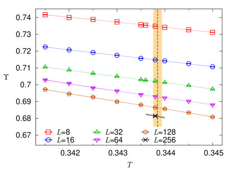
Figure 3: (Color online) QMC estimates of $\Upsilon$ for several lattice sizes $L$ up to $L=256$. For $L\leq 128$, the lines are interpolations of the data. For $L=256$, $\Upsilon$ was only computed for $T=0.3438$: the reported line corresponds to an extrapolation that uses the first two terms of the expansion of $\Upsilon$ around $T=0.3438$. The vertical band shows the final estimate $T_{c}=0.34385(9)$.

Table 1: Results for $\widetilde{T}(L)$ and $\lambda(L)$ as obtained by solving Eq. (39). We also report $T_{c}$ as obtained by linear fits to $\widetilde{T}(L)=T_{c}+c/L^{2}$ of the data satisfying $L\geq L_{\rm min}$, and the corresponding $\chi^{2}/{\rm dof}$, where dof is the number of degrees of freedom of the fit.

$L$	$\widetilde{T}(L)$	$\lambda(L)$		$L_{\rm min}$	$T_{c}$	$\chi^{2}/{\rm dof}$
4	0.34344(4)	1.457(3)		4	0.34384(3)	0.8
6	0.34380(7)	1.499(8)		6	0.34381(3)	0.4
8	0.34379(6)	1.501(9)		8	0.34382(3)	0.5
12	0.34378(6)	1.50(1)		12	0.34383(4)	0.5
16	0.34381(6)	1.51(2)		16	0.34384(5)	0.6
24	0.34378(9)	1.50(3)		24	0.34389(7)	0.5
32	0.34381(6)	1.51(3)		32	0.34390(9)	0.6
48	0.34376(11)	1.48(6)		48	0.34397(15)	0.8
64	0.34399(11)	1.61(7)		64	0.34378(22)	0.1
96	0.34385(15)	1.6(1)
128	0.34387(24)	1.5(2)

Table 2: Estimates of $T_{c}$ and $\lambda$ obtained by minimizing the functions (40) (superscript 1) and (41) (superscript 2), varying the minimal value $L_{\rm min}$ of the size allowed in the fits. We also report $s^{(i)}\equiv A^{(i)}_{\rm min}/(N_{L}-N_{f})$, where $A_{\rm min}$ is the minimum of the function $A^{(i)}$, cf. Eqs. (40), (41), $N_{L}$ and $N_{f}$ are the number of $L$-values used and the number of fit parameters, respectively.

$L_{\rm min}$	$T_{c}^{(1)}$	$\lambda^{(1)}$	$s^{(1)}$	$T_{c}^{(2)}$	$\lambda^{(2)}$	$s^{(2)}$
4	0.34374(3)	1.484(5)	8.8	0.34387(2)	1.532(7)	1.5
6	0.34380(1)	1.502(2)	0.6	0.34382(2)	1.510(6)	0.5
8	0.34381(1)	1.504(2)	0.5	0.34382(2)	1.508(8)	0.6
12	0.34381(1)	1.504(4)	0.6	0.34385(4)	1.527(14)	0.6
16	0.34382(2)	1.509(6)	0.5	0.34385(4)	1.53(2)	0.6
32	0.34384(3)	1.517(14)	0.7	0.34393(8)	1.59(6)	0.7
64	0.34389(6)	1.55(4)	0.9	0.34370(25)	1.4(2)	1.0
96	0.34373(21)	1.42(17)	1.6
128	0.34374(15)	1.41(12)	0.8

We estimate $T_{c}$ in the BH model, by using the matching method discussed above. The most accurate results are obtained by analyzing the helicity modulus $\Upsilon$. Fig. 3 shows the QMC estimates of $\Upsilon$ versus $T$ up to $L=256$. Note that they do not show any particular feature which may hint at a critical point. For instance, $T_{c}$ cannot be estimated by using the crossing-point method, as is usually done in FSS analyses of standard phase transitions, e.g., in the three-dimensional BH model.CTV-13

This is due to a peculiar feature of the behavior of RG invariant quantities at the BKT transition. Usually, the large-$L$ limit of $R(L,T)$ is discontinuous at $T_{c}$, with i.e., three different results are obtained in the limit $L\to\infty$, depending whether $T<T_{c}$, $T=T_{c}$, $T>T_{c}$, i.e.

$$\lim_{T\to T_{c}^{\pm}}\lim_{L\to\infty}R(L,T)\neq\lim_{L\to\infty}R(L,T_{c}).$$ (37)

As a consequence, for finite values of $L$, this discontinuity appears as a crossing of the finite-size curves around $T_{c}$. In the case of the 2D XY universality class, instead, the infinite-volume limit shows no discontinuity as $T$ approaches $T_{c}$ from the low-temperature side, i.e.

$$\lim_{T\to T_{c}^{-}}\lim_{L\to\infty}R(L,T)=\lim_{L\to\infty}R(L,T_{c}).$$ (38)

Hence, a crossing of the finite-size curves does not necessarily occur (it may still be present if scaling corrections have different signs on the two sides of the transition, but this does not occur for $\Upsilon$).

We implement the matching methods using various procedures, to crosscheck the results. The simplest one considers the data for only two lattice sizes at once, $L$ and $2L$. Then, $\lambda(L)$ and an effective critical temperature $\widetilde{T}(L)$ are determined by solving the two equations

$$\Upsilon[L,\widetilde{T}(L)]=\widetilde{\Upsilon}_{\rm XY}(\lambda(L)L),$$

$$\Upsilon[2L,\widetilde{T}(L)]=\widetilde{\Upsilon}_{\rm XY}(2\lambda(L)L).$$ (39)

To implement this strategy, we need accurate estimates of $\Upsilon$ in a sufficiently wide temperature interval close to $T_{c}$ for each value of $L$. For this purpose, we performed QMC simulations at relatively close values of $T$ and computed the first and second derivatives of $\Upsilon$ with respect to $T$, obtaining accurate interpolations close to the BKT transition. The results of the the two-point matching procedure based on Eqs. (39) are reported in Table 1. They appear quite stable, indicating that the residual power-law scaling corrections are small. Indeed, the solutions $\widetilde{T}(L)$ of Eqs. (39) are expected to approach $T_{c}$ with corrections of order $L^{-2}$. To take them into account, we fit $\widetilde{T}(L)$ to $T_{c}+c/L^{2}$, including only data satisfying $L\geq L_{\rm min}$. Results are stable, essentially independent of $L_{\rm min}$, confirming that the neglected scaling corrections are irrelevant within our typical error bars.

Instead of using only two lattice sizes at each step of the matching procedure, one may adopt a more general strategy in which all results satisfying $L\geq L_{\rm min}$ are used at once. In this alternative approach, $T_{c}$ and $\lambda$ are determined by minimizing the $\chi^{2}$-like function

$$A^{(1)}(T,\lambda)=\sum_{i}\left[{\Upsilon(L_{i},T)-\widetilde{\Upsilon}_{\rm XY}(\lambda L_{i})\over\Delta\Upsilon(L_{i},T)}\right]^{2},$$ (40)

where the sum is over the available lattice sizes, and $\Upsilon(L_{i},T)$ and $\Delta\Upsilon(L_{i},T)$ are the intepolating curves with their errors. In order to take into account the expected $O(L^{-2})$ corrections, we also consider

$$A^{(2)}(T,\lambda,c)=\sum_{i}\left[{\Upsilon(L_{i},T)-\widetilde{\Upsilon}_{\rm XY}(\lambda L_{i})-c/L_{i}^{2}\over\Delta\Upsilon(L_{i},T)}\right]^{2}.$$ (41)

In Table 2 we report the results. Indicative errors on the optimal parameters $T_{c}$ and $\lambda$ are obtained from the covariance matrix at the minimum of the functions (40) and (41), although this does not take into account all statistical correlations of the quantities involved in the matching procedure. The role of the residual scaling corrections is checked by increasing the minimal value $L_{\rm min}$ of the sizes considered in the fit, and by comparing the results obtained by using (40) and (41). It is clear that they are negligible.

Overall, the results of the analyses are quite stable. They indicate

$$0.3438\lesssim T_{c}(\mu=0)\lesssim 0.3439,$$ (42)

and $1.50\lesssim\lambda\lesssim 1.55$. Fig. 4 shows the quality of the matching procedure. We report the BH estimates of $\Upsilon$ at $T=0.3438\approx T_{c}$ and the critical XY curve $\widetilde{\Upsilon}_{\rm XY}(\lambda L)$, assuming $\lambda=1.5$. The BH data fall on top of the XY curve, indicating that the nonuniversal corrections of order $L^{-2}$ are quite small. In Fig. 4 we also report the asymptotic prediction (34) with constants (35). A comparison with the XY curve $\widetilde{\Upsilon}_{XY}(L)$ shows that it describes the finite-size behavior of $\Upsilon$ only for $w^{-1}\lesssim 0.05$, hence for lattice sizes which are much larger than those we simulated, up to $L=256$. Therefore, logarithmic fits to Eq. (34), i.e. including only the leading logarithmic correction, would not provide an accurate estimate for $T_{c}$.

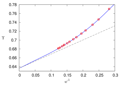
Figure 4: (Color online) Plot of the BH estimates (circles) of $\Upsilon$ at $T=0.3438\approx T_{c}$, of the finite-size curve $\widetilde{\Upsilon}_{\rm XY}(L)$ (full line), and of the asymptotic prediction (34) with constants (35) (dashed line). We take $\lambda=1.5$ and set [see Eq. (33)] $w\equiv\ln(L/\Lambda)+{1\over 2}\ln\ln(L/\Lambda)$ with $\Lambda_{\rm XY}=0.3$ for the XY model and $\Lambda_{BH}=\Lambda_{\rm XY}/\lambda=0.2$ for the BH model.

The estimate (42) is confirmed by the data of $X\equiv\xi/L$. At $T_{c}$ we expect the asymptotic behavior

$$X(L,T_{c})=\widetilde{X}_{\rm XY}(\lambda L)+cL^{-7/4},$$ (43)

which includes the expected $O(L^{-2+\eta})$ leading scaling corrections. The curve $\widetilde{X}_{\rm XY}(L)$ is reported in App. C. Note that the rescaling $\lambda$ must be the same as that obtained from the matching of $\Upsilon$, thus $\lambda\approx 1.5$. In Fig. 5 we compare the QMC estimates of $X$ at $T=0.3438$ in the BH model with the XY curve $\widetilde{X}_{\rm XY}(\lambda L)$ with $\lambda=1.5$. Note that no adjustable parameters enter this comparison. Here scaling corrections are quite larger than those observed for the helicity modulus. Nonetheless, it is quite evident that Eq. (43) holds asymptotically, and that deviations scale as $L^{-7/4}$, as predicted by theory. In the figure, we also compare the BH data with the asymptotic expression (34) [coefficients are given in Eq. (36)]. In this case, the asymptotic prediction is close to the curve $\widetilde{X}_{\rm XY}(L)$, indicating that, once the power-law scaling corrections become negligible, a logarithmic fit would provide the correct estimate of $T_{c}$.

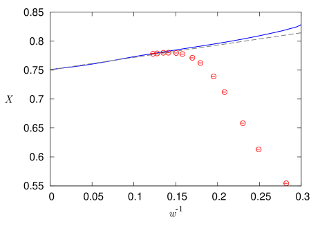
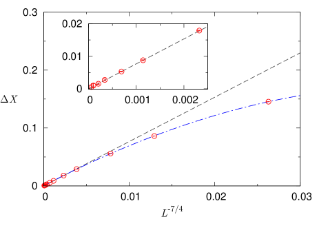
Figure 5: (Color online) Top: Plot of the BH estimates (circles) of $X\equiv\xi/L$ at $T=0.3438\approx T_{c}$, of the XY function $\widetilde{X}_{\rm XY}(L)$ (full line), and of the asymptotic prediction (34) with constants (36) (dashed line). We use $\lambda=1.5$ and set [see Eq. (33)] $w\equiv\ln(L/\Lambda)+{1\over 2}\ln\ln(L/\Lambda)$ with $\Lambda_{\rm XY}=0.3$ for the XY model and $\Lambda_{BH}=\Lambda_{\rm XY}/\lambda=0.2$ for the BH model. Bottom: Difference $\Delta X=\widetilde{X}_{\rm XY}(\lambda L)-X(L,T_{c})$ for $\lambda=1.5$. The dashed line is a linear fit to $aL^{-7/4}$ of the data satisfying $L\geq 24$. The dotted-dashed line shows a fit to $aL^{-7/4}+bL^{-2}+cL^{-4}$ of the data for $L\geq 8$, which takes also into account the expected higher-order power-law corrections.

II.4.3 A more general analysis

Table 3: Estimates of $T_{c}$ and $\lambda$ obtained by fitting the data to Eq. (45) (superscript 1) and to Eq. (47) (superscript 2), varying the minimal value $L_{\rm min}$ of the size allowed in the analyses.

$L_{\rm min}$	$T_{c}^{(1)}$	$\lambda^{(1)}$	$T_{c}^{(2)}$	$\lambda^{(2)}$
6	0.34384(2)	1.52(1)	0.34384(2)	1.52(1)
8	0.34385(2)	1.52(1)	0.34384(2)	1.52(1)
12	0.34386(3)	1.53(2)	0.34385(3)	1.53(2)
16	0.34386(3)	1.53(2)	0.34386(3)	1.53(2)
24	0.34386(3)	1.54(2)	0.34386(5)	1.53(3)

The two analyses presented in Sec. II.4.2 are straightforward implementations of the matching procedure. However, they require interpolations of the data at fixed size and an estimation of the error on the interpolations. One can avoid both steps, by slightly generalizing the matching procedure. For the values of $T$ that we consider and for each size $L$, the helicity modulus is an almost linear function of $T$, as is clear from Fig. 3. Therefore, we can expand $\Upsilon(L,T)$ as

$$\Upsilon(L,T)\approx\Upsilon(L,T_{c})+(T-T_{c})\left.{\partial\Upsilon\over\partial T}\right|_{T=T_{c}}.$$ (44)

Now, we use the matching condition to relate $\Upsilon(L,T_{c})$ to the corresponding XY quantity. Including the leading scaling corrections we obtain

$$\Upsilon(L,T)\approx\widetilde{\Upsilon}_{\rm XY}(\lambda L)+(T-T_{c})\left.{\partial\Upsilon\over\partial T}\right|_{T=T_{c}}+c/L^{2}.$$ (45)

This relation is at the basis of two different analyses of the BH data, that differ in the treatment of the derivative term.

In the first analysis we use the QMC results for $\partial\Upsilon/\partial T$. Within errors, the estimates of the derivative appear to be essentially independent of $T$ for $T$ close to 0.3438. Hence, to obtain a reliable interpolation we simply consider all data in the interval $0.343\leq T\leq 0.345$ and determine an interpolation of the form

$$S(L)\equiv\left.{\partial\Upsilon\over\partial T}\right|_{T=T_{c}}=w\sum_{k=0}^{n}\alpha_{k}w^{-k}+{c_{T}\over L^{2}},$$ (46)

where $w$ is defined in Eq. (33) and we take $\Lambda=\Lambda_{\rm XY}/\lambda=0.2$ (we take $\Lambda_{\rm XY}=0.3$, consistently with the estimates reported in App. C). The interpolating function is consistent with the RG results of App. A, which predict $\partial\Upsilon/\partial T\sim\ln L$ at the critical point. We try several values of $n$, obtaining an almost perfect interpolation for $n\geq 3$. Once the interpolation is known, we determine $T_{c}$ and $\lambda$ by fitting all BH data to Eq. (45), taking $\lambda$, $T_{c}$, and $c$ as free parameters. The fit is repeated several times, including each time only the data satisfying $L\geq L_{\rm min}$, for an increasing sequence of $L_{\rm min}$. The results are reported in Table 3. We only take into account the statistical errors and, in particular, we neglect the uncertainty on the interpolation of the derivative of $\Upsilon$. Therefore, errors may be (slightly) underestimated. The results are perfectly consistent with those reported in Sec. II.4.2 and confirm Eq. (42).

We also performed a second fit, in which the QMC results for the derivative of $\Upsilon$ are not used. We only assume that an expression like (46) provides an accurate interpolation. Therefore, we performed fits to

$$\Upsilon(L,T)=\widetilde{\Upsilon}_{\rm XY}(\lambda L)+{c\over L^{2}}+$$

$$\quad(T-T_{c})\left(\alpha_{0}h(L,\lambda)+\alpha_{1}+{\alpha_{2}\over h(L,\lambda)}+{c_{T}\over L^{2}}\right),$$ (47)

with

$$h(L,\lambda)=\ln{\lambda L\over\Lambda_{\rm XY}}+{1\over 2}\ln\ln{\lambda L\over\Lambda_{\rm XY}},$$ (48)

and $\Lambda_{\rm XY}=0.3$. In the fit, $\lambda$, $T_{c}$, $\alpha_{0}$, $\alpha_{1}$, $\alpha_{2}$, $c$, and $c_{T}$ are free parameters. The results are reported in Table 3. In spite of the quite large number of parameters, results are stable and completely consistent with those obtained by using the interpolation of the temperature derivative. Again, they confirm Eq. (42).

II.4.4 Final estimate of the critical temperature

In the analyses presented in Sections II.4.2 and II.4.3 we made the implicit assumption that the exact curve for the helicity modulus at criticality is known. But this is not the case. There are two sources of uncertainty. First, the interpolations are affected by an error related to the statistical error of the XY data. As discussed in App. C, this error is quite small. The relative uncertainty is less than $3\times 10^{-5}$ for $L\lesssim 400$, which is the relevant region for the analysis of the BH data. This source of error is practically irrelevant, since it changes the results of the fits by a small fraction of the statistical error. For the analyses presented in Sec. II.4.3, $T_{c}$ varies by at most $4\times 10^{-6}$, if we change the curve by one error bar.

On the other hand, the error on the critical XY temperature gives rise to systematic deviations on our final results which are not negligible and which are of the order of the statistical errors. To estimate the corresponding systematic error, let us indicate with $\beta_{\rm XY}=1.1199$ ($T_{\rm XY}=1/\beta_{\rm XY}$), which is the value at which we computed the XY function $\widetilde{\Upsilon}_{\rm XY}(L)$, and with $T_{c,\rm XY}$ the true XY critical temperature. If $\sigma=T_{c,\rm XY}-T_{\rm XY}$ is small, we can write

$$\Upsilon_{\rm XY}(T_{c,\rm XY},L) \approx \Upsilon_{\rm XY}(T_{\rm XY},L)+\sigma S_{\rm XY}(L)$$ (49)

$$= \widetilde{\Upsilon}_{\rm XY}(L)+\sigma S_{\rm XY}(L),$$

where $S_{\rm XY}(L)=\partial\Upsilon_{\rm XY}/\partial T$ computed at the critical point. For the BH model we can write analogously

$$\Upsilon_{\rm BH}(T,L)=\Upsilon_{BH}(T_{c,{\rm BH}},L)+(T-T_{c,{\rm BH}})S_{\rm BH}(L).$$ (50)

We can now use the matching conditions (20) and (22) to rewrite the previous relation as

$$\Upsilon_{\rm BH}(T,L)=\Upsilon_{\rm XY}(T_{c,{\rm XY}},\lambda L)+{1\over k}(T-T_{c,{\rm BH}})S_{\rm XY}(\lambda L).$$ (51)

Finally, Eq. (49) implies

$$\Upsilon_{BH}(T,L)=\widetilde{\Upsilon}_{\rm XY}(\lambda L)+\left[{1\over k}(T-T_{c,{\rm BH}})+\sigma\right]S_{\rm XY}(\lambda L).$$ (52)

In our approach, we compute the value of $T$ which provides the best matching between $\Upsilon_{\rm BH}(T,L)$ and $\widetilde{\Upsilon}_{\rm XY}(\lambda L)$. It corresponds to the value of $T$ for which the correction term vanishes, hence

$$T=T_{c,{\rm BH}}-k\sigma.$$ (53)

Therefore, the systematic error on our estimates of the critical temperature of the BH model is $|k\sigma|$, where $\sigma$ is the error on $T_{c,\rm XY}$: $\beta_{\rm XY}^{2}\sigma=10^{-4}$. To compute the nonuniversal constant $k$, we perform runs for the XY model at $\beta=1.1201$ and a few values of $L$, obtaining estimates of $S_{\rm XY}(L)$. Comparing this results with the BH ones, we estimate $k/\beta_{\rm XY}^{2}=0.6(1)$, which gives

$$k\sigma\lesssim 7\cdot 10^{-5}.$$ (54)

If we now assume that the statistical error and the systematic error due to the uncertainty on $T_{c,\rm XY}$ are independent, we obtain the final estimate

$$T_{c}=0.34385(9).$$ (55)

To conclude, we compare our result (55) with the estimates of $T_{c}$ reported in the literature for the 2D hard-core BH model at $\mu=0$: $T_{c}=0.3425(5)$ is reported in Ref. CR-12, , $T_{c}=0.3423(3)$ in Ref. HK-97, , $T_{c}=0.353(3)$ in Ref. Ding-92, , and $T_{c}=0.350(4)$ in Ref. DM-90, . There are significant discrepancies with our result (55); we believe that this is essentially due to the residual logarithmic corrections affecting the extrapolation of the numerical data in Refs. CR-12, ; HK-97, ; Ding-92, ; DM-90, . Other numerical results for generic 2D BH models can be found in Refs. EM-99, ; CSPS-08, ; PKVT-08, ; RBRS-09, ; MDKKST-11, ; CT-12, ; YLFCW-12, .

III BKT critical behavior in a trap

Experimental evidences of BKT transitions in trapped quasi-2D atomic gases have been reported in Refs. HKCBD-06, ; KHD-07, ; HKCRD-08, ; CRRHP-09, ; HZGC-10, ; Pl-etal-11, ; Desb-etal-12, . The inhomogeneity due to the trapping potential drastically changes, even qualitatively, the general features of the BKT critical behavior. The analysis of the RG flow in the presence of a trapping potential leads to nontrivial scaling laws characterized by the presence of additional logarithmic factors.PV-13 Here, we discuss the results of QMC simulations of the 2D hard-core BH model in the presence of a harmonic trapping potential. We verify the RG predictions, and in particular the universality of the trap-size dependence at the critical temperature.

III.1 Trap-size dependence

In sufficiently smooth inhomogeneous systems, the trap-size dependence of the particle density $\rho({\bf x})\equiv\langle n_{\bf x}\rangle$ can be approximately obtained by using the local-density approximation (LDA). In this approach, $\rho({\bf x})$ is approximately given by the value of the particle density of the homogeneous system at the same temperature and at an effective chemical potential

$$\mu_{\rm eff}({\bf x})=\mu-V(r)=\mu-(r/\ell_{t})^{2}.$$ (56)

Thus, the LDA implies that the particle density depends on the ratio $r/\ell_{t}$ and that the total particle number asymptotically scales as

$$N=\sum_{\bf x}\rho({\bf x})\approx c(\mu)\ell_{t}^{2},$$ (57)

with a coefficient that depends on $\mu$. Actually, the LDA is expected to give the exact space dependence of the particle density in the large-$\ell_{t}$ limit keeping $r/\ell_{t}$ fixed. Scaling corrections decay as inverse powers of $\ell_{t}$, CV-10-2 ; CTV-12 and are generally determined by the universal features of the critical behavior.CV-10 ; CTV-13

The main features of the critical behavior are encoded in the correlation functions of the critical modes, like the one-particle correlation function, whose leading behavior shows a nonanalytic TSS around the critical point. We consider the one-particle correlation function between the center of the trap ${\bf x}=0$ and another point ${\bf y}$, i.e.

$$G_{0}({\bf y})\equiv G({\bf 0},{\bf y})\equiv\langle b_{\bf 0}^{\dagger}b_{\bf y}\rangle.$$ (58)

We also define the trap susceptibility

$$\chi_{t}=\sum_{\bf x}G_{0}({\bf x}),$$ (59)

(it differs from the usual susceptibility $\chi$, which considers correlations between any pair of points in the lattice), and the trap correlation length $\xi_{t}$ defined in terms of the second moment of $G_{0}({\bf x})$:

$$\xi_{t}^{2}={1\over 4\chi_{t}}\sum_{\bf x}|{\bf x}|^{2}G_{0}({\bf x}).$$ (60)

At the BKT transition the TSS of $G_{0}({\bf x})$ presents multiplicative logarithms,PV-13

$$G_{0}({\bf x})=\ell_{t}^{-1/4}(\ln\ell_{t})^{1/8+\kappa/4}\,{\cal G}\left[{\bf x}(\ln\ell_{t})^{\kappa}/\ell_{t}\right],$$ (61)

where $\kappa$ is a new exponent related to the trap, which is expected to depend on the main features of the external potential. In the inhomogeneous XY model (7), $\kappa$ depends on the power $q$ of the link function (8). Numerical results provide evidence of a simple dependence: PV-13

$$\kappa=2/q.$$ (62)

Eq. (61) implies the scaling relations at $T_{c}$

$$\chi_{t}\sim\ell_{t}^{7/4}(\ln\ell_{t})^{1/8-7\kappa/4},$$ (63)

$$\xi_{t}\sim\ell_{t}(\ln\ell_{t})^{-\kappa}.$$ (64)

Note that the exponent $\kappa$ must vanish in the limit $q\to\infty$. Indeed, for $q\to\infty$, one is dealing with a homogeneous system with open boundary conditions. Hence, one should recover the usual FSS relations with $\ell_{t}\sim L$.

We would like to note that the additional logarithmic factors are a specific feature of the BKT point. Indeed, in the low-temperature QLRO phase the trap-size dependence is simpler. The correlation length satisfies $\xi_{t}\sim\ell_{t}$ without logarithms,CV-11 and the one-particle correlation function scales as

$$G_{0}({\bf x})=\ell_{t}^{-\eta(T)}{\cal G}\left({\bf x}/\ell_{t}\right),$$ (65)

with $\eta(T)<1/4$.

III.2 Universality of the trap-size scaling

A major physical question concerns the universality of the trap effects, i.e. under which conditions critical exponents and scaling functions are the same for different trapped systems that belong to the same “homogeneous” universality class.

Let us begin by discussing which features of the trapping potential are relevant in the TSS limit. Consider a generic model with trapping potential $V(r/\ell_{t})$ where $r$ is the distance from the center of the trap. The TSS limit is obtained by taking $r\to\infty$, $\ell_{t}\to\infty$ at fixed $\zeta=r/\ell_{t}^{\theta}$, where $\theta$ is the trap exponent. Therefore, since $r/\ell_{t}=\zeta\ell^{\theta-1}_{t}$, if $\theta<1$ as generically occurs, in the TSS limit the argument of the potential tends to zero: only the small-$r$ behavior, i.e., the one for $r\ll\ell_{t}$, is relevant. For the XY model we have $\theta=1$ with logarithmic corrections controlled by the exponent $\kappa$.PV-13 In this case, $\zeta=r(\ln\ell_{t})^{\kappa}/\ell_{t}$, so that $r/\ell_{t}=\zeta/(\ln\ell_{t})^{\kappa}$. Therefore, provided that $\kappa>0$, also in this case the relevant behavior is the small-distance one. As a consequence, if $V(r/\ell_{t})\approx(r/\ell_{t})^{p}$ for $r\to 0$, in all cases we expect TSS to depend only on $p$ and not on more specific features of the potential.

In Ref. PV-13, scaling functions and exponent $\kappa$ were computed for the XY model (7) with link function $W(r)$ given in Eq. (8). They depend on the exponent $q$. In particular, results were consistent with $\kappa=2/q$. Since $\kappa>0$, they confirm that only the small-distance behavior of $W(r)$ is relevant in the TSS limit. Since the BH model and the XY model belong to same universality class in homogeneous conditions, the trap-size behavior in the two models is expected to be strictly related.

Since the small-$r$ behavior is the relevant property that characterizes the universality class in the presence of the trap, it seems natural to assume that the trapped BH model and the classical inhomogeneous XY model have the same TSS at $T_{c}$ when $p=q$, i.e., when the trapping potential $V(r)$ and the link variable $W_{ij}(r)$ have the same short-distance behavior. However, the scaling argument presented below, which is confirmed by our numerical results, shows that this is not always true. In particular, we argue that, at $\mu=0$, the correct correspondence is $q=2p$.

For homogeneous systems, in the absence of a magnetic field, the relevant quantity that controls the critical behavior of the 2D XY model is the temperature difference $\tau=T-T_{c}$. In the inhomogeneous case, cf. Eq. (7), we can associate an effective temperature $T_{\rm eff}(r)$ to each point at distance $r$ from the center of the trap. Then, we argue that two inhomogeneous systems have the same TSS provided that the short-distance behavior of the relevant RG perturbation $\tau(r)=T_{\rm eff}(r)-T_{c}$ is the same. In the case of the classical XY model at $T_{c}$, we have $\tau(r)\sim W(r)\sim r^{q}$. In the case of the hard-core BH model at $T=T_{c}(\mu)$, we have

$$\tau(r)\equiv T_{c}(\mu)-T_{c}[\mu_{\rm eff}(r)],$$ (66)

where the effective chemical potential is given in Eq. (56). Now, for $\mu\not=0$ and $\delta\mu\ll 1$,

$$T_{c}(\mu+\delta\mu)-T_{c}(\mu)\sim\delta\mu.$$ (67)

Therefore, at least for values of $r$ for which $V(r)\ll\mu$ (this is the relevant region in the TSS limit, as discussed above), we obtain $\tau(r)\sim V(r)\sim r^{p}$. Therefore, we expect the same TSS for $p=q$. This result, however, does not apply to the case $\mu=0$, due to the symmetry properties of the phase diagram reported in Fig. 1. Because of the symmetry under $\mu\to-\mu$, we have for $\mu\to 0$

$$T_{c}(\mu)=T_{c}(0)+c\mu^{2}+O(\mu^{4}).$$ (68)

Then, by using again Eq. (56), we obtain $\tau(r)\sim V(r)^{2}\sim r^{2p}$, which implies that, for $\mu=0$ the correct correspondence is $q=2p$. This argument allows us to predict that, for the BH model with $p=2$, the exponent $\kappa$ should be equal to 1 for $\mu\not=0$ and to 1/2 for $\mu=0$.

The equality of the short-distance behavior of the effective $\tau(r)$ appears to be a necessary requirement for two systems to belong to the same TSS universality class. If this condition holds, critical exponents are the same. For the scaling functions however, a more careful analysis is needed. Indeed, in homogeneous systems, the critical behavior depends on the phase: critical exponents are always the same, but scaling functions in the high- and low-temperature phase differ. Hence, when comparing scaling functions, one must be careful to perform the comparison for systems that are in the same effective phase. It is therefore important to understand the effective behavior in the inhomogeneous XY and BH models.

In the trapped hard-core BH model with $\mu\leq 0$ and the XY model (7), the external field brings the system toward the high-temperature phase when moving out of the center of the trap. In the XY model (7) the effective space-dependent temperature defined in Eq. (9) tends to infinity when $r\equiv|{\bf x}|\to\infty$; in particular, for $T=T_{c}$, $T_{\rm eff}({\bf x})>T_{c}$ for any $r>0$. Analogously, in the BH model one may define the effective space-dependent chemical potential (56). When $\mu\leq 0$ and $T=T_{c}$, the phase diagram (1) is such that the system is effectively in the high-temperature phase for any $r>0$. Therefore, the hard-core BH model with $\mu\leq 0$ and in the inhomogenous XY model (7) should share the same universal features. The two model should share the same TSS scaling functions, provided the exponents satisfy the relations discussed above.

The behavior for $\mu>0$ is expected to be different. Since the trapping potential decreases the local effective chemical potential (56), the system is in the superfluid QLRO phase for $0<r\lesssim\sqrt{2\mu}\ell_{t}$, and in the normal phase only for $r\gtrsim\sqrt{2\mu}\ell_{t}$. In the TSS limit at $\zeta=r(\ln\ell_{t})^{\kappa}/\ell_{t}$ fixed, we expect a low-temperature behavior for $\zeta\lesssim\sqrt{2\mu}(\ln\ell_{t})^{\kappa}$. Since $\kappa>0$, as $\ell_{t}$ increases, the boundary of the QLRO phase goes to infinity: In the TSS limit all points belong to the QLRO phase. Therefore, even if the TSS logarithmic exponent is the same as in the case $\mu<0$, scaling functions for $\mu>0$ should differ from those obtained for $\mu<0$. Actually, we guess that the TSS functions at $\mu>0$ should correspond to those of the inhomogenous XY model (7) with $U_{{\bf x}{\bf y}}=[1+W(r_{{\bf x}{\bf y}})]^{-1}$ replaced by $U_{{\bf x}{\bf y}}=1+W(r_{{\bf x}{\bf y}})$.

An analogous scenario is also expected in the three-dimensional (3D) hard-core BH model, whose phase diagram is similar to that reported in Fig. 1, with a finite-temperature XY superfluid transition line from ($\mu=-3,T=0$) to ($\mu=3,T=0$). Again this transition line is symmetric with respect to $\mu\to-\mu$, therefore $T_{c}(\mu)$ has a maximum at $\mu=0$. The TSS at the superfluid transition is generally characterized by the trap exponent CV-09 $\theta=p\nu/(1+p\nu)$ for a trapping potential $V(r)=(r/\ell_{t})^{p}$, where $\nu=0.6717(1)$ is the correlation-length exponent of the 3D XY universality class.CHPV-06 This is confirmed by a numerical study CTV-13 of the 3D BH model with a harmonic trapping potential at $\mu=-2$, for which $\theta=0.57327(4)$. This result is expected to hold for all values of $\mu$ between $-3$ and $3$ that are different from zero. At the particular value $\mu=0$, the argument outlined above implies that the trap exponent is different, being associated with an external field given by $V(r)^{2}=(r/\ell_{t})^{2p}$. Therefore,CV-09 we expect $\theta=2p\nu/(1+2p\nu)$, giving $\theta=0.72876(3)$ for $p=2$. Finally, note that, although we expect $\theta=0.57327(4)$ for any $\mu\not=0$, scaling functions should depend on the sign of $\mu$.

III.3 QMC results

Figure 6: (Color online) Comparison of $G_{0}({\bf x})$ versus $r=|{\bf x}|$ for several trap sizes $\ell_{t}$ and lattice sizes $L$, at $T=0.3438\approx T_{c}$. No size dependence is observed for $L\gtrsim 4\ell_{t}$.

Figure 7: (Color online) The particle density at $T=0.3438\approx T_{c}$ for several trap sizes versus $r/\ell_{t}$ (data obtained taking $L\gtrsim 4\ell_{t}$). Data collapse onto a unique curve.

Figure 8: (Color online) The connected density-density correlation $G_{n}(0,{\bf x})$ at $T=0.3438\approx T_{c}$ for several trap sizes, versus $r\equiv|{\bf x}|$.

We numerically check the RG predictions of the previous section by performing QMC simulations of the 2D hard-core BH model (4) at $\mu=0$ and $T=0.3438\approx T_{c}$, with a harmonic potential [$p=2$ in Eq. (5)]. We present results for several values of the trap size $\ell_{t}$, up to $\ell_{t}=32$. The trap is centered in the middle of a square $L^{2}$ lattice, with odd $L$ and open boundary conditions. More details on our practical implementation of QMC simulations of trapped systems can be found in Refs. CTV-12, ; CT-12, .

The lattice size $L$ is large enough ($L\approx 4\ell_{t}$) to make finite-size effects negligible compared with the statistical errors, at least for the critical correlations with respect to the center of the trap. This is checked by comparing results for several lattice sizes $L$ at fixed trap size $\ell_{t}$. In Fig. 6 we show the one-particle correlation function $G_{0}({\bf x})$. Within the precision of our data, results obtained by using lattice sizes $L=4\ell_{t}+1$ — i.e. $L/\ell_{t}\approx 4$ — can be identified as infinite-volume results.

Figure 9: (Color online) Scaling of the one-particle correlation function $G_{0}({\bf x})$ in a trap, using Eq. (61) with $\kappa=0$ (top, note that this is analogous to the rescaling of the distance for the particle density, as in Fig. 7), $\kappa=1$ (middle) and $\kappa=1/2$ (bottom). The value $\kappa=1/2$ is clearly favoured by the data, supporting the RG arguments of Sec. III.2. All results are obtained for $L=4\ell_{t}+1$. footnoteftss

In Fig. 7 we show the particle density $\rho({\bf x})\equiv\langle n_{\bf x}\rangle$ at $T_{c}$. The data collapse onto a single curve when plotted as a function of the rescaled distance $r/\ell_{t}$. The large-$\ell_{t}$ convergence at fixed ratio $r/\ell_{t}$ is quite fast; one can hardly see variations for $\ell_{t}\geq 8$ already. These results are consistent with the LDA, as discussed in Sec. III.1. In particular, we find $\rho(0)\approx 1/2$ (we obtain $\rho(0)=0.5006(3),\;0.4999(3),\;0.5004(4)$ respectively for $\ell_{t}=8,\,16,\,32$), which is the particle density of the homogeneous system at $\mu=0$, cf. Eq. (10). The data in Fig. 7 show also that, at $T=0.3438$ and $\mu=0$, the particles are effectively confined within a spherical region $|{\bf x}|\lesssim 2\ell_{t}$ by the harmonic potential (indeed $\rho\approx 10^{-4}$ for $r\approx 2\ell_{t}$).

The connected density-density correlation

$$G_{n}({\bf 0},{\bf x})\equiv\langle n_{\bf 0}n_{\bf x}\rangle-\langle n_{\bf 0}\rangle\langle n_{\bf x}\rangle$$ (69)

vanishes rapidly, see Fig. 8, without showing any particular scaling behavior. This is analogous to the behavior observed in the one-dimensional BH model in the zero-temperature quantum superfluid phase.CTV-12 Notice that the value $G_{n}(0,0)\approx 1/4$ at the center of trap (we obtain $G_{n}(0,0)=1/4$ for any $\ell_{t}$ with a precision of $10^{-6}$) agrees with the corresponding LDA prediction. Indeed, it corresponds to the value $G_{n}({\bf x},{\bf x})=1/4$ in homogeneous systems at zero chemical potential.footnotegrho

Fig. 9 shows QMC data for the one-particle correlation function $G_{0}({\bf x})$. They are rescaled using Eq. (61), with $\kappa=0,\,1/2$, and 1. The best collapse of the data is observed for $\kappa=1/2$, supporting the RG arguments of the previous section. In Fig. 10 we show the trap correlation length $\xi_{t}$. The data are consistent with the asymptotic behavior with $\kappa=1/2$, i.e., with

$$\xi_{t}\sim\ell_{t}(\ln\ell_{t})^{-1/2}.$$ (70)

Figure 10: (Color online) QMC data of the second-moment correlation length at $T=0.3438\approx T_{c}$ versus $\ell_{t}(\ln\ell_{t})^{-\kappa}$, with $\kappa=1/2$. The dotted straight line is drawn to guide the eye.

We now perform a more stringent universality check, verifying that the hard-core BH model with $p=2$ and the classical XY model at $T_{\rm XY}$ with $q=4$ have the same TSS. To avoid the use of free parameters, we plot the correlation functions in terms of the universal ratio $r/\xi_{t}$ instead of $r/\ell_{t}$, and consider $G_{0}({\bf x})/Z_{t}$, $Z_{t}\equiv\chi_{t}/\xi_{t}^{2}$, and $G_{0}(2{\bf x})/G_{0}({\bf x})$. With these choices, the nonuniversal normalization of the correlation function cancels out. In Fig. 11 we compare the BH results for these two quantities with the corresponding data for the classical XY model (7) with $q=2$ and $q=4$. The XY data obtained by using $q=4$ fall on top of the BH results, while those obtained by using $q=2$ differ significantly. Hence, these results provide a nice evidence for the correspondence $q=2p$, as argued in the previous section.

Figure 11: (Color online) Universality check at $T_{c}$: plot of $Z_{t}^{-1}G_{0}(x)$ with $Z_{t}=\chi_{t}/\xi_{t}^{2}$ (top) and of the ratio $G_{0}(2r)/G_{0}(r)$ (bottom) vs $r/\xi_{t}$ with $r\equiv|x|$, for the trapped hard-core BH model with $p=2$, and for the classical XY model with $q=4$ and $q=2$. In both cases the data for the harmonically ($p=2$) trapped BH model converge to the large-$\ell_{t}$ curve of the classical XY model with a quartic external field ($q=4$). In the bottom panel the horizontal dashed line gives the $r\to\ 0$ limit (in the continuum limit).

IV Conclusions

We investigate the universal behavior of quantum 2D many-body systems at finite-temperature BKT transitions. We consider the 2D hard-core BH model (I) [which is equivalent to the so-called XX spin model (2)] in homogeneous conditions and in the presence of a harmonic trap, cf. Eq. (4). The phase diagram, sketched in Fig. 1, presents a BKT transition line between the normal and superfluid QLRO phase. We consider the system at half filling ($\mu=0$), performing extensive QMC simulations. We first perform a detailed FSS analysis to determine the critical temperature and then a detailed check of the TSS RG predictions.

In order to determine the critical BKT temperature, we employ a numerical matching method, which relates the FSS of RG invariant quantities in the 2D BH model with that in the classical XY model (3) at its critical temperature, which is known with high accuracy.HP-97 ; Hasenbusch-05 In this approach, the residual scaling corrections decay as inverse powers of the lattice size $L$ and not as powers of $1/\ln L$, as in more standard approaches. Therefore, it allows us to perform reliable large-$L$ extrapolations and to obtain accurate and robust estimates of the critical temperature. This procedure yields $T_{c}(\mu=0)=0.34385(9)$, which significantly improves earlier estimates.CR-12 ; HK-97 ; Ding-92 ; DM-90

We stress that the matching method can be used to determine the critical temperature of any physical system undergoing a BKT transition, using the XY finite-size curves reported in App. C. The precision of the method is essentially limited by the relative precision of the estimate $\beta_{\rm XY}=1.1199(1)$ of the XY critical temperature. This limitation may be overcome by computing the relevant FSS curves in the BCSOS model, for which $T_{c}$ is exactly known.Baxter-82 ; HMP-94

The matching method is quite general and can be used in other systems characterized by marginal RG perturbations, as long as an accurate estimate of the critical temperature for at least one representative of the given universality class is known. For instance, one could apply it to the study of three-dimensional tricritical transitions, of $\Phi^{4}$ scalar models in four dimensions,It-Dr-book of the quantum $T=0$ Mott transition of the 2D BH model,FWGF-89 ; SSS-94 or of two-dimensional randomly dilute Ising systems.RandomlyDilute ; HPPV-08

We also investigate the universal BKT behavior in the presence of a harmonic trap, cf. Eq. (4). In this case the trap exponent takes the trivial value $\theta=1$, but, additionally, logarithmic corrections appear. PV-13 At the critical BKT temperature the correlation length $\xi_{t}$ scales as $\xi_{t}\sim\ell_{t}(\ln\ell_{t})^{-\kappa}$ with respect to the trap size $\ell_{t}$, where the exponent $\kappa$ depends on the general features of the external trapping potential. For the classical XY model with an effective space-dependent temperature $T_{\rm eff}(T,{\bf x})=T[1+(r/\ell_{t})^{q}]$, numerical simulations PV-13 suggested the relation $\kappa=2/q$. We argue, and provide numerical evidence, that the trapped BH models and this inhomogeneous XY model share universal features. The exponent $\kappa$ should generally be equal to $2/p$ [$p$ is defined in Eq. (5)], hence we should have $\kappa=1$ for a harmonic potential. This result does not apply to the particular case of the hard-core BH model at zero chemical potential. We argue that in this case the BH model with potential exponent $p$ is in the universality class of the XY model with $q=2p$. Hence $\kappa=1/2$ for $p=2$. Note that, although the exponent $\kappa$ is the same for any $\mu\not=0$, scaling functions are expected to depend on the sign of $\mu$.

To verify the theoretical arguments, we perform extensive QMC simulations of the hard-core BH model at $\mu=0$. We consider several trap sizes, up to $\ell_{t}=32$, measuring the one-particle correlation function $G_{0}({\bf x})=\langle b_{0}^{\dagger}b_{\bf x}\rangle$ between the center of the trap ${\bf 0}$ and a generic point ${\bf x}$. A careful analysis of the numerical results, presented in Sec. III.3, confirms the scaling arguments, in particular the correspondence between the BH model with $p=2$ with the XY model with $q=4$.

The results we present in this paper are relevant for experiments probing BKT transitions, both in homogeneous systems, such as ⁴He at the superfluid transition,GKMD-08 and in inhomogeneous systems, such as cold atoms in harmonic traps.BDZ-08 In particular, experimental results for the one-particle correlation function of quasi-2D trapped atomic gases can be inferred from the interferences between two atomic clouds.HKCBD-06 ; CRRHP-09 The analysis of experimental data reported in Ref. HKCBD-06, provided some evidence of an algebraic decay in the superfluid regime HKCBD-06 , although trap effects were effectively neglected.

Accurate studies of the critical properties of trapped systems, to check universality and determine the critical exponents, require a robust control of the effects of the confining potential. Our results should be useful to determine the critical parameters of the BKT transition, without requiring further assumptions and approximations, such as mean-field and local-density approximations, to handle the inhomogeneity arising from the trapping force. In particular, in trapped quasi-2D particle systems one may exploit the difference of the trap-size dependence of the critical correlation functions between the high- and low-temperature phases: with decreasing $T$ we go from the normal phase, in which the trap-size dependence is trivial, to the QLRO phase where the length scale increases proportionally to the trap size, through the BKT transition where the relation between $\xi_{t}$ and $\ell_{t}$ shows also multiplicative logarithms, $\xi_{t}\sim\ell_{t}(\ln\ell_{t})^{-\kappa}$.

Appendix A Off-critical finite-size scaling: renormalization-group predictions

In Ref. PV-13, we investigated the FSS behavior at the BKT critical point. We wish now to discuss the nature of the off-critical corrections. For a standard phase transition, these corrections can be expressed in power series of $\tau L^{1/\nu}$, $\tau=(T-T_{c})/T_{c}$. Therefore, critical-point scaling holds as long as $\tau L^{1/\nu}\ll 1$. Since formally $\nu=\infty$, in the XY model we expect some expansion in terms of $\tau\ln^{\alpha}L$. We wish now to show that this guess is correct and moreover we wish to compute the exponent $\alpha$. We find

$$\alpha=2.$$ (71)

We start from the flow of $v(l)$ with $l_{0}=\ln L$ (notations are those of Ref. PV-13, ):

$$\ln L=\int_{v(L)}^{v_{0}}{dw\over[Q+F(w)](1+wf(w^{2}))}.$$ (72)

If we now consider the leading term for $Q\to 0$ and $L\to\infty$, we obtain

$$\ln L\approx\int_{v(L)}^{v_{0}}{dw\over[Q+w^{2}]}={1\over\sqrt{Q}}\left({\rm arctan}{v_{0}\over\sqrt{Q}}-{\rm arctan}{v\over\sqrt{Q}}\right).$$ (73)

It follows

$$v(L)={v_{0}-\sqrt{Q}\tan(\sqrt{Q}\ln L)\over 1+v_{0}\tan(\sqrt{Q}\ln L)/\sqrt{Q}}.$$ (74)

In order to obtain critical-point behavior, we should assume that $\sqrt{Q}\ln L\ll 1$. Since $Q\sim\tau$, this implies $\tau\ln^{2}L\ll 1$, which proves the relation $\alpha=2$. If we now expand the previous relation in powers of $\sqrt{Q}\ln L$, we obtain the first-order temperature correction:

$$v(L)={v_{0}\over 1+v_{0}\ln L}-{Q\over 3}{\ln L(v_{0}^{2}\ln^{2}L+3v_{0}\ln L+3)\over(1+v_{0}\ln L)^{2}}.$$ (75)

If we now consider the infinite-volume limit, this gives

$$v(L)={1\over\ln L}\left(1-{Q\ln^{2}L\over 3}\right)+\ldots$$ (76)

Let us now consider a renormalization-group quantity $R$, which satisfies

$$R(Q,v_{0},L)=R(Q,v(L),1).$$ (77)

Expanding this scaling equation in powers of $Q$ and $v$, we find

$$R(Q,v_{0},L) = R^{*}+av(L)+bQ$$ (78)

$$\approx R^{*}+{a\over\ln L}\left(1-{Q\ln^{2}L\over 3}\right)+\ldots$$

Since $Q\sim(T-T_{c})$, this relation implies

$$\left.{\partial R\over\partial T}\right|_{T_{c}}=-{a\alpha_{1}\over 3}\ln L$$ (79)

for $L\to\infty$.

Appendix B Exact relations within the QLRO phase

The critical behavior of systems with $U(1)$ symmetry in the QLRO low-temperature phase can be obtained by studying the Gaussian spin-wave theory

$$H={\beta\over 2}\int d^{2}x\,(\nabla\varphi)^{2}.$$ (80)

The relevant two-point function is

$$G({\bf x}_{1},{\bf x}_{2})=\langle e^{-i\varphi({\bf x}_{1})}e^{i\varphi({\bf x}_{2})}\rangle.$$ (81)

A simple calculation shows that, in the infinite-volume limit, $G({\bf x}_{1},{\bf x}_{2})\sim|{\bf x}_{1}-{\bf x}_{2}|^{-\eta}$, where the exponent $\eta$ is related to the coupling $\beta$ by

$$\eta={1\over 2\pi\beta}.$$ (82)

This spin-wave theory describes the QLRO phase of 2D U(1)-symmetric models for $\beta\geq 2/\pi$, corresponding to $0\leq\eta\leq 1/4$. The values $\beta=2/\pi$ and $\eta=1/4$ correspond to the BKT transition.

Let us now consider the system on a finite $L\times L$ square with periodic boundary conditions. The two-point function for the Gaussian theory with periodic boundary conditions can be exactly computed, obtaining CFT-book ; It-Dr-book

$$G_{\rm sw}({\bf x})=\left[{e^{\pi z_{2}^{2}}\theta^{\prime}_{1}(0,e^{-\pi})\over|\theta_{1}[\pi(z_{1}+iz_{2}),e^{-\pi}]|}\right]^{\eta},$$ (83)

where $z_{i}\equiv x_{i}/L$, $\theta_{1}(u,q)$ and $\theta_{1}^{\prime}(u,q)$ are $\theta$ functions.Gradstein However, in the original model the field $\varphi$ is periodic, hence the XY model with periodic boundary conditions is equivalent to the Gaussian theory, provided one sums over all twisted boundary conditions, i.e. over all configurations satisfying $\varphi(L)=\varphi(0)+2n\pi$, $n$ arbitrary integer. This effect can be taken into account by the following formula:Hasenbusch-05 ; CFT-book

$$G({\bf x})=G_{\rm sw}({\bf x})\times$$ (84)

$$\quad{\sum_{n_{1},n_{2}=-\infty}^{\infty}W(n_{1},n_{2})\cos[2\pi(n_{1}x_{1}+n_{2}x_{2})]\over\sum_{n_{1},n_{2}=-\infty}^{\infty}W(n_{1},n_{2})},$$

$$W(n_{1},n_{2})=\exp[-\pi(n_{1}^{2}+n_{2}^{2})/\eta].$$

Using Eq. (83) and this expression, we can compute the universal function $X(\eta)$, where $X\equiv\xi/L$ and

$$\xi^{2}={L^{2}\over 4\pi^{2}}\left({\chi\over\chi_{1}}-1\right),$$ (85)

$$\chi=\int d^{2}x\,G({\bf x}),\quad\chi_{1}=\int d^{2}x\,{\rm cos}\left({2\pi x_{1}\over L}\right)\,G({\bf x}).$$

The curve $X(\eta)$ is shown in Fig. 2. In particular, close to the BKT point, i.e., for $\eta\to 1/4$, we obtain

$$X(\eta)=0.7506912222+1.699451\,\left({1\over 4}-\eta\right)+\ldots$$ (86)

which is in agreement with the numerical results reported in Ref. Hasenbusch-05, . Analogous results have been obtained for the helicity modulus,Hasenbusch-05

$$\Upsilon(\eta)={1\over 2\pi\eta}-{\sum_{n=-\infty}^{\infty}n^{2}\,{\rm exp}(-\pi n^{2}/\eta)\over\eta^{2}\sum_{n=-\infty}^{\infty}{\rm exp}(-\pi n^{2}/\eta)}=$$ (87)

$$=0.6365081782+2.551196\,\left({1\over 4}-\eta\right)+...$$

The asymptotic behaviors (34) for $X$ and $\Upsilon$ are obtained by noting Hasenbusch-05 that $1/4-\eta\approx 1/(8w)$ for $w\to\infty$ and $\eta\to 1/4$.

Appendix C XY finite-size curves

We consider the classical XY model (3) at $\beta_{\rm XY}\equiv 1/T_{\rm XY}=1.1199$ (which is the best available estimateHP-97 of the critical temperature), on $L\times L$ square lattices with periodic boundary conditions. We determine accurate approximations of the functions $\widetilde{\Upsilon}_{\rm XY}(L)$ and $\widetilde{X}_{\rm XY}(L)$, by interpolating the available Monte Carlo data Hasenbusch-05 ; Hasenbusch-08 at $\beta_{\rm XY}=1.1199$, which cover the interval $4\leq L\leq 4096$. Moreover, we also enforce the known large-$L$ asymptotic behaviors (34), (35) and (36), to guarantee the correct limit $L\to\infty$. We consider functional forms motivated by theory. Hence, the functions $\widetilde{Y}_{\rm XY}(L)$ and $\widetilde{X}_{\rm XY}(L)$ are expressed as polynomials in the variable $w\equiv\ln({L/\Lambda})+{1\over 2}\ln\ln(L/\Lambda)$, plus some correction terms of order $L^{-2k}$. In practice, we approximate the two functions as

$$\sum_{k=0}^{n}a_{k}/w^{k}+\sum_{k=1}^{m}b_{k}L^{-2k}.$$ (88)

In the case of $\widetilde{X}$ we also add a term $cL^{-7/4}$, as suggested by the correction-to-scaling analysis presented in Sec. II.2. Coefficients $a_{0}$ and $a_{1}$ are fixed by using Eqs. (34), (35) and (36), while the others are obtained by fitting the data.

First, we performed several fits, changing the orders of the polynomials $n$ and $m$, and considering the scale $\Lambda$ as a free parameter. We obtained almost perfect interpolations by taking $n=5$ and $m=3$. We also observed that the fits of $X$ and $\Upsilon$ were providing very similar values for the scale $\Lambda$. With the previous choices of $n$ and $m$, we obtained $\Lambda\approx 0.31$ from the analysis of $\Upsilon$ and $\Lambda\approx 0.34$ from the analysis of $X$. Similar values where obtained in fits in which $n$ and $m$ were slightly changed. The consistency of the two results confirms the adequacy of our interpolating expressions. To obtain the final interpolations we fixed $\Lambda=0.3$ for both quantities, obtaining

$$\widetilde{\Upsilon}_{\rm XY}(L) = 0.6365081782+0.318899454\,w^{-1}$$

$$+ 2.0319176\,w^{-2}-40.492461\,w^{-3}$$

$$+ 325.66533\,w^{-4}-874.77113\,w^{-5}$$

$$+ 8.43794\,L^{-2}+79.1227\,L^{-4}-210.217\,L^{-6},$$

and

$$\widetilde{X}_{\rm XY}(L) = 0.7506912222+0.21243137\,w^{-1}$$

$$- 2.8971137\,w^{-2}+76.328276\,w^{-3}$$

$$- 642.23425\,w^{-4}+1805.3274w^{-5}$$

$$- 1.879629\,L^{-7/4}-15.00621\,L^{-2}$$

$$- 196.205\,L^{-4}+805.644\,L^{-6}.$$

It is important to note that these expressions have the only purpose of providing an accurate interpolation of the numerical data, and are not meant to provide the correct large-$L$ asymptotic behavior. For instance, they should not be used to estimate the coefficient of the corrections proportional to $1/\ln^{2}L\sim w^{-2}$: $a_{2}$ obtained in the fit probably differs significantly from the correct large-$L$ coefficient.

The uncertainty on the interpolation curves is related to the errors on the available Monte Carlo data. It depends on $L$ and can be evaluated by using a bootstrap method, which yields the curves shown in Fig. 12. Errors are almost constant and very small up to $L\approx 10^{3}$, i.e., in the region in which we have data, then they increase, reaching a maximum for $L\approx 10^{8}$. Eventually, they should decrease to zero as $1/(\ln L)^{2}$, due to the fact that the interpolations have the correct asymptotic behavior (34).

Figure 12: (Color online) Plot of the errors on the curves (C) and (C).

References

- (1) J. M. Kosterlitz and D. J. Thouless, J. Phys. C: Solid State 6, 1181 (1973)
- (2) V. L. Berezinskii, Zh. Eksp. Theor. Fiz. 59, 907 (1970) [Sov. Phys. JETP 32, 493 (1971)].
- (3) J. M. Kosterlitz, J. Phys. C 7, 1046 (1974).
- (4) J. V. José, L. P. Kadanoff, S. Kirkpatrick, and D. R. Nelson, Phys. Rev. B 16, 1217 (1977).
- (5) N. D. Mermin and H. Wagner, Phys. Rev. Lett. 17, 1133 (1966).
- (6) P. C. Hohenberg, Phys. Rev. 158, 383 (1967).
- (7) D. J. Bishop and J. D. Reppy, Phys. Rev. Lett. 40, 1727 (1978).
- (8) F. M. Gasparini, M. O. Kimball, K. P. Mooney, and M. Diaz-Avilla, Rev. Mod. Phys. 80, 1009 (2008).
- (9) D. J. Resnick, J. C. Garland, J. T. Boyd, S. Shoemaker, and R. S. Newrock, Phys. Rev. Lett. 47, 1542 (1981).
- (10) Z. Hadzibabic, P. Krüger, M. Cheneau, B. Battelier, and J. Dalibard, Nature 441, 1118 (2006).
- (11) P. Krüger, Z. Hadzibabic, and J. Dalibard, Phys. Rev. Lett. 99, 040402 (2007).
- (12) Z. Hadzibabic, P. Krüger, M. Cheneau, S. P. Rath, and J. Dalibard, New J. Phys. 10, 045006 (2008).
- (13) P. Cladé, C. Ryu, A. Ramanathan, K. Helmerson, and W. D. Phillips, Phys. Rev. Lett. 102, 170401 (2009).
- (14) C.-L. Hung, X. Zhang, N. Gemelke, and C. Chin, Nature 470, 236 (2011).
- (15) T. Plisson, B. Allard, M. Holzmann, G. Salomon, A. Aspect, P. Bouyer, and T. Bourdel, Phys. Rev. A 84, 061606(R) (2011).
- (16) R. Desbuquois, L. Chomaz, T. Yefsah, J. Léonard, J. Beugnon, C. Weitenberg, and J. Dalibard, Nature Phys. 8, 645 (2012).
- (17) I. Bloch, J. Dalibard, and W. Zwerger, Rev. Mod. Phys. 80, 885 (2008).
- (18) D. Jaksch, C. Bruder, J. I. Cirac, C. W. Gardiner, and P. Zoller, Phys. Rev. Lett. 81, 3108 (1998).
- (19) M. P. A. Fisher, P. B. Weichman, G. Grinstein, and D. S. Fisher, Phys. Rev. B 40, 546 (1989).
- (20) The spin operators are related to the boson operators by , , .
- (21) D. J. Amit, Y. Y. Goldschmidt, and G. Grinstein, J. Phys. A 13, 585 (1980).
- (22) M. Hasenbusch, M. Marcu, and K. Pinn, Physica A 208, 124 (1994).
- (23) M. Hasenbusch and K. Pinn, J. Phys. A 30, 63 (1997).
- (24) J. Balog, J. Phys. A 34, 5237 (2001).
- (25) M. Hasenbusch, J. Phys. A 38, 5869 (2005).
- (26) A. Pelissetto and E. Vicari, Phys. Rev. E 87, 032105 (2013).
- (27) M. Hasenbusch, J. Stat. Mech.: Theory Expt. P08003 (2008).
- (28) M. Hasenbusch, J. Stat. Mech.: Theory Expt. P02005 (2009).
- (29) M. Hasenbusch, Phys. Rev. B 85, 174421 (2012).
- (30) Y. Komura and Y. Okabe, J. Phys. Soc. Jpn. 81, 113001 (2012).
- (31) Y.-D. Hsieh, Y.-J. Kao, and A. W. Sandvik, arXiv:1302.2900.
- (32) E. A. Cornell and C. E. Wieman, Rev. Mod. Phys. 74, 875 (2002); N. Ketterle, Rev. Mod. Phys. 74, 1131 (2002).
- (33) J. Carrasquilla and M. Rigol, Phys. Rev. A 86, 043629 (2012).
- (34) M. Holzmann and W. Krauth, Phys. Rev. Lett. 100, 190402 (2008).
- (35) M. Campostrini and E. Vicari, Phys. Rev. Lett. 102, 240601 (2009); (E) 103, 269901 (2009).
- (36) M. Campostrini and E. Vicari, Phys. Rev. A 81, 023606 (2010).
- (37) F. Crecchi and E. Vicari, Phys. Rev. A 83, 035602 (2011).
- (38) A. W. Sandvik, Phys. Rev. B 59, R14157 (1999).
- (39) O. F. Syljuasen, and A. W. Sandvik, Phys. Rev. E 66, 046701 (2002).
- (40) A. Dorneich, M. Troyer, Phys. Rev. E 64, 066701 (2001).
- (41) Typical statistics of the runs range from to Monte Carlo steps, where a Monte Carlo step is made of one diagonal update and off-diagonal updates. The number is estimated at run time and turns out to linearly increase with .
- (42) M. Campostrini, M. Hasenbusch, A. Pelissetto, and E. Vicari, Phys. Rev. B 74, 144506 (2006).
- (43) The helicity modulus is related to the change of the partition function under twists of the boundary conditions along one of the lattice directions, i.e. .
- (44) A. W. Sandvik, Phys. Rev. B 56, 11678 (1997).
- (45) M. E. Fisher, M. N. Barber, and D. Jasnow, Phys. Rev. A 8, 1111 (1973).
- (46) E. L. Pollock and D. M. Ceperley, Phys. Rev. B 36, 8343 (1987).
- (47) A. Pelissetto and E. Vicari, Phys. Rep. 368, 549 (2002).
- (48) M. Hasenbusch, A. Pelissetto, and E. Vicari, J. Stat. Mech.: Theory Expt. P12002 (2005).
- (49) K. Harada and N. Kawashima, Phys. Rev. B 55, R11949 (1997).
- (50) H.-Q. Ding, Phys. Rev. B 45, 230 (1992).
- (51) H.-Q. Ding and M.S. Makivić, Phys. Rev. B 42, 6827 (1990).
- (52) G. Ceccarelli, C. Torrero, and E. Vicari, Phys. Rev. B 87, 024513 (2013).
- (53) N. Elstner and H. Monien, Phys. Rev. B 59, 12184 (1999).
- (54) B. Capogrosso-Sansone, S. G. Soÿler, N. V. Prokof’ev, and B. V. Svistunov, Phys. Rev. A 77, 015602 (2008).
- (55) L. Pollet, C. Kollath, K. Van Houche, and M. Troyer, New J. Phys. 10, 065001 (2008).
- (56) M. Rigol, G. G. Batrouni, V. G. Rousseau, and R. T. Scalettar, Phys. Rev. A 79, 053605 (2009).
- (57) K.W. Mahmud, E. N. Duchon, Y. Kato, N. Kawashima, R. T. Scalettar, and N. Trivedi, Phys. Rev. B 84, 054302 (2011).
- (58) G. Ceccarelli and C. Torrero, Phys. Rev. A 85, 053637 (2012).
- (59) J.-S. You, H. Lee, S. Fang, M.A. Cazalilla, and D.-W. Wang, Phys. Rev. A 86, 043612 (2012).
- (60) M. Campostrini and E. Vicari, Phys. Rev. A 81, 063614 (2010).
- (61) G. Ceccarelli, C. Torrero, and E. Vicari, Phys. Rev. A 85, 023616 (2012).
- (62) This can be easily proved within the equivalent XX model (2), using at and .
- (63) Since the correlation length scales as , finite-size effects in the critical quantities (related to the ratio ) should further decrease keeping the ratio constant while increasing .
- (64) R. J. Baxter, Exactly Solved Models in Statistical Mechanics, (Academic, New York, 1982).
- (65) C. Itzykson and J. M. Drouffe, Statistical Field Theory (Cambridge Univ. Press, Cambridge, 1989).
- (66) S. Sachdev, T. Senthil, and R. Shankar, Phys. Rev. B 50, 258 (1994).
- (67) B. N. Shalaev, Sov. Phys. Solid State 26, 1811 (1984); R. Shankar, Phys. Rev. Lett. 58, 2466 (1987); A. W. W. Ludwig, Nucl. Phys. B 330, 639 (1990).
- (68) M. Hasenbusch, F. Parisen Toldin, A. Pelissetto, and E. Vicari, Phys. Rev. E 78, 011110 (2008).
- (69) P. Di Francesco, P. Mathieu, and D. Senechal, Conformal Field Theory (Springer Verlag, New York, 1997).
- (70) I. S. Gradshteyn and I. M. Ryzhik, Table of Integrals, Series, and Products, edited by A. Jeffrey and D. Zwillinger, 7th edition (Academic Press, San Diego, 2007).