Optimal Sensor and Actuator Placement in
Complex Dynamical Networks

Abstract

Controllability and observability have long been recognized as fundamental structural properties of dynamical systems, but have recently seen renewed interest in the context of large, complex networks of dynamical systems. A basic problem is sensor and actuator placement: choose a subset from a finite set of possible placements to optimize some real-valued controllability and observability metrics of the network. Surprisingly little is known about the structure of such combinatorial optimization problems. In this paper, we show that an important class of metrics based on the controllability and observability Gramians has a strong structural property that allows efficient global optimization: the mapping from possible placements to the trace of the associated Gramian is a modular set function. We illustrate the results via placement of power electronic actuators in a model of the European power grid.

I Introduction

Controllability and observability have been recognized as fundamental structural properties of dynamical systems since the seminal work of Kalman in 1960 [13], but have recently seen renewed interest in the context of large, complex networks, such as power grids, the Internet, transportation networks, and social networks. A prominent example of this recent interest is [16], which, based on Kalman’s rank condition and the idea of structural controllability, presents a graph theoretic maximum matching method to efficiently identify a minimal set of so-called driver nodes through which time-varying control inputs can move the system around the entire state space (i.e., render the system controllable). The method of [16] is applied across a range of technological and social systems, leading to several interesting and surprising conclusions. Using a metric of controllability given by the fraction of driver nodes in the minimal set required for complete controllability, it is shown that sparse inhomogeneous networks are difficult to control while dense homogeneous networks are easier. It is also shown that the minimum number of driver nodes is determined mainly by the degree distribution of the network. Many other studies of controllability in complex networks have followed, including [20, 19, 23, 24, 21].

One issue with the approach taken by [16] and much of the follow up work is that the quantitative notion of controllability discussed in [16] (namely, the number/fraction of required driver nodes) is rather crude in some settings. This was noted, for example, by [18] in response to the surprising result in [16] that genetic regulatory networks seem to require many driver nodes, which apparently contradicts other findings in biological literature on cellular reprogramming. Rather than finding a set of driver nodes that would render a network completely controllable, a more appropriate strategy might be to choose from a finite set of possible actuators and sensors placements to optimize some real-valued controllability and observability metrics of the network, which is not considered in [16]. There is a variety of more sophisticated metrics for controllability and observability that have been proposed in the systems and control literature on sensor and actuator placement or selection problems in dynamical systems; see, e.g., the survey paper [22]. One important class of metrics involves the controllability and observability Gramians, which are symmetric positive semidefinite matrices whose structure defines energy-related notions of controllability and observability.

While a variety of metrics have been proposed [22], the corresponding combinatorial optimization problems for sensor and actuator placement are less well-understood. These can be solved by brute force for small problems by testing all possible placement combinations. However, for problems that arise in large networks, testing all combinations quickly becomes infeasible and so the problems are generally thought to be very difficult combinatorial optimization problems, requiring inefficient integer programming techniques in general. Some techniques based on efficient $\ell_{1}$ heuristics have been proposed, e.g. [10], but it is not clear when they work.

In the present paper, we show that one important class of metrics of controllability and observability, previously thought to lead to difficult combinatorial optimization problems [22], can be in fact easily optimized, even for very large networks. In particular, we show that the mapping from subsets of possible actuator/sensor placements to any linear function of the associated controllability or observability Gramian has a strong structural property: it is a modular set function. We also describe how this observation defines a new dynamic network centrality measure for networks whose dynamics are described by linear models, assigning a control energy-related “importance” value to each node in the network. We illustrate the results in power electronic actuator placement in a model of the European power grid.

The rest of the paper is organized as follows. Section II reviews basics of linear dynamical systems and controllability. Section III introduces the notions of modular, submodular, and supermodular set functions and shows that the set function mapping possible actuator placements to any linear function of the controllability Gramian is modular. Section IV presents a case study in a power network. Section V gives concluding remarks and and outlook for future research.

II Linear Models of Network Dynamics

This section defines a linear model for network dynamics and reviews and interprets metrics for controllability based on the controllability Gramian. The material in this section is mostly standard and can be found in many texts on linear system theory, e.g. [11, 2]; we discuss the material mostly to set our notation. Since controllability and observability are dual properties [12], we focus only on controllability; all of the results have analogous counterparts and interpretations for observability.

While virtually all real systems have nonlinear dynamics, there is a local structural equivalence between nonlinear models and associated linearized models (via the Hartman-Grobman theorem), and the resulting linear models are widely used across many engineering and science disciplines. We therefore focus on linear, time-invariant dynamical network models, in which the dynamics are given by

$$\dot{x}(t) =Ax(t)+Bu(t),\quad x(0)=x_{0},$$ (1)

$$y(t) =Cx(t)$$

where $x(t)\in\mathbf{R}^{n}$ represents the state of the network and $u(t)\in\mathbf{R}^{m}$ represents the control inputs that can be used to influence the networks dynamics. For example, $x(t)$ might represent voltages, currents, or frequencies in devices in a power grid, species concentrations in a genetic regulatory network, or individual opinions or propensities for product adoption in a social network. The dynamics matrix induces a graph on the nodes of the network: there is an edge between two nodes $i$ and $j$ if $a_{ij}$ is non-zero. The matrix $C\in\mathbf{R}^{p\times n}$ is typically interpreted as a set of linear state measurements, but here we will interpret it as a weight matrix whose rows define important directions in the state space.

II-A Controllability

Definition 1 (Controllability)

A dynamical system is called controllable over a time interval $[0,t]$ if given any states $x_{0}$, $x_{1}\in\mathbf{R}^{n}$, there exists an input $u(\cdot):[0,t]\rightarrow\mathbf{R}^{m}$ that drives the system from $x_{0}$ at time $0$ to $x_{1}$ at time $t$.

Kalman’s well-known rank condition states that a linear dynamical system is controllable if and only if $[B,AB,...,A^{n-1}B]$ is full rank. Since rank is a generic property of a matrix, it has the same value for almost all values of the non-zero entries of $A$ and $B$ (assuming that the non-zero entries are independent). The controllability property is thus at its core a structural property of the graph defined by $A$ and $B$, as captured in the graph-theoretic concept of structural controllability described by Lin in [15], which underpins the recent results of [16]. However, while Kalman’s rank condition is widely used, it only gives a binary metric for controllability. It is interesting to consider more sophisticated quantitative metrics for controllability in complex networks.

II-B An energy-related controllability metric

Every actuator in a real system is energy limited, so an important class of metrics of controllability deals with the amount of input energy required to reach a given state from the origin. In particular, we can pose the following optimal control problem seeking the minimum energy input that drives the system from the origin to a final state $x_{f}$ at time $t$:

$$\underset{{u(\cdot)\in\mathcal{L}_{2}}}{\text{minimize}} \int_{0}^{t}\|u(\tau)\|^{2}d\tau$$ (2)

subject to $$\dot{x}(t)=Ax(t)+Bu(t),$$

$$x(0)=0,\quad x(t)=x_{f}$$

Standard methods from optimal control theory can be used to derive the solution. If the system is controllable, the optimal input has the form

$$u^{*}(\tau)=B^{T}e^{A^{T}(t-\tau)} \left(\int_{0}^{t}e^{A\sigma}BB^{T}e^{A^{T}\sigma}d\sigma\right)^{-1}x_{f},$$ (3)

$$0\leq\tau\leq t$$

and the resulting minimum energy is

$$\int_{0}^{t}\|u^{*}(\tau)\|^{2}d\tau=x_{f}^{T}\left(\int_{0}^{t}e^{A\sigma}BB^{T}e^{A^{T}\sigma}d\sigma\right)^{-1}x_{f}.$$ (4)

The matrix

$$W_{c}(t)=\int_{0}^{t}e^{A\tau}BB^{T}e^{A^{T}\tau}d\tau\ \in\mathbf{R}^{n\times n}$$ (5)

is called the controllability Gramian at time $t$. The controllability Gramian is positive semidefinite and has the same rank as $[B,AB,...,A^{n-1}B]$. It defines an ellipsoid in the state space

$$\mathcal{E}_{min}(t)=\left\{x\in\mathbf{R}^{n}|x^{T}W_{c}(t)^{-1}x\leq 1\right\}$$ (6)

that contains the set of states reachable in $t$ seconds with one unit or less of input energy. The eigenvectors and corresponding eigenvalues of $W_{c}$ define the semi-axes and corresponding semi-axis lengths of the ellipsoid. Eigenvectors of $W_{c}$ associated small eigenvalues (large eigenvalues of $W_{c}^{-1}$) define directions in the state space that are less controllable (require large input energy to reach), and eigenvectors of $W_{c}$ associated with large eigenvalues (small eigenvalues of $W_{c}^{-1}$) define directions in the state space that are more controllable (require small input energy to reach).

For stable systems, the state transition matrix $e^{At}$ comprises decaying exponentials, so a finite positive definite limit of the controllability Gramian always exists and is given by

$$W_{c}=\int_{0}^{\infty}e^{A\tau}BB^{T}e^{A^{T}\tau}d\tau\ \in\mathbf{R}^{n\times n}$$ (7)

This matrix defines an ellipsoid in the state space that gives the states reachable with one unit or less of energy, regardless of time. This infinite-horizon controllability Gramian can be computed by solving a Lyapunov equation

$$AW_{c}+W_{c}A^{T}+BB^{T}=0,$$ (8)

which is a system of linear equations and is therefore easily solvable, even for large systems. Specialized algorithms have been developed to compute the solution; see, e.g., [1, 8].

The controllability Gramian gives a more sophisticated energy-related quantitative picture of controllability, but we still need to form a scalar metric for $W_{c}$, which is a positive semidefinite matrix. We want $W_{c}$ “large” so that $W_{c}^{-1}$ is “small”, requiring small amount of input energy to move around the state space. There are a number of possible metrics for the size of $W_{c}$, including minimum eigenvalue, determinant, trace, sums/products of the first $k$ eigenvalues, etc.. We focus here on the trace metric, which as we show below, has interesting interpretations in terms of average energy and linear system norms and has a strong structural property for actuator placement problems.

II-C Interpretations of trace$(W_{c})$

Average Energy: The average value of the minimum control energy over the unit hypersphere is proportional to the trace of $W_{c}^{-1}$:

$$\frac{\int_{\|x\|=1}x^{T}W_{c}^{-1}xdx}{\int_{\|x\|=1}dx}=\frac{1}{n}\textbf{tr}W_{c}^{-1}.$$ (9)

The trace of $W_{c}$ is inversely related to the trace of $W_{c}^{-1}$, so maximizing $\textbf{tr}(W_{c})$ effectively minimizes the average energy required to move around the state space in all directions. Maximizing a weighted trace, representing any linear function of a matrix, minimizes a weighted average energy required to move around the state space, with certain directions weighted differently, which can be encoded into the $C$ matrix.

System $H_{2}$ norm: An important norm of a (stable) linear dynamical system is defined as

$$\|H\|_{2}=\left(\textbf{tr}\frac{1}{2\pi}\int_{-\infty}^{\infty}H(j\omega)H(j\omega)^{*}d\omega\right)^{1/2}.$$ (10)

This can be interpreted as the RMS response of the system when it is driven by a white noise input. By the Parseval theorem, this is also given by

$$\|H\|_{2}=\left(\textbf{tr}\int_{0}^{\infty}h(t)^{T}h(t)dt\right)^{1/2}=\|h(t)\|_{2},$$ (11)

where $h(t)=Ce^{At}B$ is the impulse response matrix. Thus, the $H_{2}$ norm can also be interpreted as the $L_{2}$ norm, or energy, of the system response to a unit impulse input.

The connection between the system $H_{2}$ norm and the controllability Gramian can be seen as follows:

$$\|H\|_{2}^{2} =\textbf{tr}\left(\int_{0}^{\infty}h(t)h(t)^{T}dt\right)$$ (12)

$$=\textbf{tr}\left(C\int_{0}^{\infty}e^{At}BB^{T}e^{A^{T}t}dtC^{T}\right)$$

$$=\textbf{tr}(CW_{c}C^{T})$$

i.e., the system $H_{2}$ norm is a weighted trace of the controllability Gramian.

III Optimal Sensor and Actuator Placement in Networks

III-A Set Functions, Modularity, and Submodularity

Sensor and actuator placement problems can be formulated as set function optimization problems. For a given finite set $V=\{1,...,M\}$, a set function $f:2^{V}\rightarrow\mathbf{R}$ assigns a real number to each subset of $V$. In our setting, the elements of $V$ represent potential locations for the placement of sensors or actuators in a dynamical system, and the function $f$ is a metric for how controllable or observable the system is for a given set of placements, which is to be maximized.

We consider set function optimization problems of the form

$$\underset{{S\subseteq V,\ |S|=k}}{\text{maximize}}\quad f(S).$$ (13)

The problem is to select a $k$-element subset of $V$ that maximizes $f$. This is a finite combinatorial optimization problem, so one way to solve it is by brute force: simply enumerate all possible subsets of size $k$, evaluate $f$, and pick the best subset. However, we are interested in cases arising from complex networks in which the number of possible subsets is very large. The number of possible subsets grows extremely fast as $V$ increases, so the brute force approach quickly becomes infeasible as $V$ becomes large.

Other approaches for solving (13) include general combinatorial optimization methods, e.g. branch and bound, and methods based on $\ell_{1}$ optimization heuristics [10]. However, general combinatorial methods do not scale well with problem size, and while $\ell_{1}$ heuristics scale well in principle, it is unclear when they work, and they provide no approximation guarantees.

Another broad approach is to exploit structural properties of the set function $f$ that make them more amenable to optimization, such as modularity and submodularity [17, 7]. Submodularity is defined as follows.

Definition 2 (Submodularity)

A set function $f:2^{V}\rightarrow\mathbf{R}$ is called submodular if for all subsets $A\subseteq B\subseteq V$ and all elements $s\notin B$, it holds that

$$f(A\cup\{s\})-f(A)\geq f(B\cup\{s\})-f(B),$$ (14)

or equivalently, if for all subsets $A,B\subseteq V$, it holds that

$$f(A)+f(B)\geq f(A\cup B)+f(A\cap B).$$ (15)

Intuitively, submodularity is a diminishing returns property where adding an element to a smaller set gives a larger gain than adding one to a larger set. A set function is called supermodular if the reversed inequalities in (14) and (15) hold, and is called modular if it is both submodular and supermodular, i.e. for all subsets $A,B\subseteq V$, we have $f(A\cap B)+f(A\cup B)=f(A)+f(B)$. A modular function has the following simple, equivalent characterization [17]:

Theorem 1 (Modularity)

A set function $f:2^{V}\rightarrow\mathbf{R}$ is modular if and only if for any subset $S\subseteq V$ it can be expressed as

$$f(S)=w(\emptyset)+\sum_{s\in S}w(s)$$ (16)

for some weight function $w:V\rightarrow\mathbf{R}$.

Modular set functions are analogous to linear functions and have the property that each element of a subset gives an independent contribution to the function value. In particular, modular functions are easily optimized: since the contribution of each element is independent, one can simply evaluate the set function for each individual element and then choose the best $k$ individual elements to obtain the best subset of size $k$.

Submodularity plays a similar role in combinatorial optimization as convexity in continuous optimization [17]. It occurs often in applications (though is underexplored in systems and control theory); is preserved under various operations, allowing design flexibility; has a beautiful and practically useful mathematical theory; and there are efficient methods for minimizing and near-optimal methods for maximizing.

We now demonstrate the modularity of a class of controllability metrics involving linear functions of the controllability Gramian.

III-B Main Result: Any linear function of the controllability Gramian is a modular set function

Suppose we are given a stable system $A$ matrix and a set of possible $B$ matrix columns $V=\{b_{1},...,b_{M}\}$. The problem is to choose a subset of the possible $B$ matrix columns to maximize a metric of controllability. Here, we consider the weighted trace of the controllability Gramian, i.e., any linear function of the controllability Gramian. For a given $S\subseteq V$, we form $B_{S}=[b_{s}],\ s\in S$ and the associated controllability Gramian $W_{S}=\int_{0}^{\infty}e^{A\tau}B_{S}B_{S}^{T}e^{A^{T}\tau}d\tau$, which is the unique positive definite solution the Lyapunov equation

$$AW_{S}+W_{S}A^{T}+B_{S}B_{S}^{T}=0.$$ (17)

To simplify notation, we write $W_{s}$ for $W_{\{s\}}$. We have the following result.

Theorem 2

Let $A\in\mathbf{R}^{n\times n}$ be a stable dynamics matrix and $V=\{b_{1},...,b_{M}\}$ be a set of possible actuator locations. The set function mapping subsets $S\subseteq V$ to any linear function of the associated controllability Gramian, i.e. $f(S)=\mathbf{tr}(\bar{C}W_{S})$ for any weighting matrix $\bar{C}\in\mathbf{R}^{n\times n}$, is modular.

Proof:

We will prove the result directly using Theorem 1. Take any $S\subseteq V$ and let $B_{S}$ denote the input matrix formed by taking the associated columns defined by $S$. Note that

$$B_{S}B_{S}^{T} =\left[\begin{array}[]{ccc}b_{s_{1}}&\cdots&b_{s_{|S|}}\end{array}\right]\left[\begin{array}[]{ccc}b_{s_{1}}&\cdots&b_{s_{|S|}}\end{array}\right]^{T}$$ (18)

$$=\sum_{s\in S}b_{s}b_{s}^{T}.$$

It is easy to see that the controllability Gramian associated with $B_{S}$ is simply a sum of the controllability Gramians associated with the individual columns of $B_{S}$:

$$W_{S} =\int_{0}^{\infty}e^{A\tau}B_{S}B_{S}^{T}e^{A^{T}\tau}d\tau$$ (19)

$$=\int_{0}^{\infty}e^{A\tau}\sum_{s\in S}b_{s}b_{s}^{T}e^{A^{T}\tau}d\tau$$

$$=\sum_{s\in S}\int_{0}^{\infty}e^{A\tau}b_{s}b_{s}^{T}e^{A^{T}\tau}d\tau$$

$$=\sum_{s\in S}W_{s}$$

Now since trace is a linear matrix function, we have for any weight matrix $\bar{C}\in\mathbf{R}^{n\times n}$

$$f(S) =\textbf{tr}(\bar{C}W_{S})$$ (20)

$$=\textbf{tr}\left(\sum_{s\in S}\bar{C}W_{s}\right)$$

$$=\sum_{s\in S}\textbf{tr}(\bar{C}W_{s})$$

Thus, for any $s\in V$, we can define the weight function $w(s)=\textbf{tr}(\bar{C}W_{s})$. Defining $w(\emptyset)=0$, Theorem 1 implies that $f(S)=\textbf{tr}(\bar{C}W_{S})$ is a modular set function. ∎

Theorem 2 shows that each possible actuator placement gives an independent contribution to the trace of the controllability Gramian. Because of this, the actuator placement problem using this metric is easily solved: one needs only to compute the metric individually for each possible actuator placement, sort the results, and choose the best $k$. Based on the interpretations in the previous section, this means that placing actuators in a complex network to maximize the average amount of controllability available to move the system around the state space, or to maximize the energy in the system response to a unit impulse, is easily done. Since the result holds for the weighted trace, this gives considerable design freedom for actuator placement; important directions in the state space can be weighted and actuator placement done based on the weighted metric.

III-C A Dynamic Network Centrality Measure

Network centrality measures are real-valued functions that assign a relative “importance” to each node within a graph. Examples include degree, betweenness, closeness, and eigenvector centrality. The meaning of importance and the relevance of various metrics depends highly on the modeling context. For example, PageRank, a variant of eigenvector centrality, turns out to be a much better indicator of importance than vertex degree in the context of networks of web pages, one of the core factors leading to Google’s domination of web search.

In the context of complex dynamical networks, the controllability metric described above can be used to define a control energy-based centrality measure, describing the importance of a node in terms of its ability to move the system around the state space with a low-energy time-varying control input. In particular, imagine that it is possible to place an actuator at each individual node in the network; thus, define $V=\{e_{1},...,e_{n}\}$, where $e_{i}$ is the standard unit basis vector in $\mathbf{R}^{n}$, i.e. $e_{i}$ has a $1$ in the $i$th entry and zeros elsewhere. We define the Control Energy Centrality for a complex dynamical network as follows.

Definition 3 (Average Energy Controllability Centrality)

Given a complex network with $n$ nodes and an associated stable linear dynamics matrix $A\in\mathbf{R}^{n\times n}$, the Average Energy Controllability Centrality measure for node $i$ is given by

$$C_{CE}(i)=\mathbf{tr}(W_{i}),\quad i\in V$$ (21)

where $W_{i}$ is the infinite-horizon controllability Gramian that satisfies $AW_{i}+W_{i}A^{T}+e_{i}e_{i}^{T}=0$.

An interesting topic for future work would be to explore the distribution of the Average Energy Controllability Centrality measure in random networks and networks from various application domains.

IV Power electronic actuator placement in the European power grid

New power electronic actuators, such as high voltage direct current (HVDC) links or flexible alternating current transmission devices (FACTS), can be used to improve transient stability properties in power grids by modulating active and reactive power injections to damp frequency oscillations and prevent rotor angle instability [4]. In this section, we illustrate the results via placement of such power electronic actuators in a model of the European power grid. We emphasize that this section is intended only to illustrate the theory in the preceding sections and show what kind of questions could be answered; many practical political and economic issues are neglected, and placements are evaluated entirely from a controllability perspective.

We consider a simplified model of the European grid derived from [9] with 74 buses, each of which is connected to a generator and a constant impedance load. We consider the placement of HVDC links, which are modeled as ideal current sources that can instantaneously inject AC currents into each bus; for modeling details see [4, 5, 6] The system dynamics we consider here are based on the swing equations, a widely-used nonlinear model for the time evolution of rotor angles and frequencies of each generator in the network [14]. Each HVDC link has three degrees of freedom that allow influence of the frequency dynamics at the corresponding buses. The nonlinear model is linearized about a desired operating condition for each possible HVDC link placement, and the placements are evaluated based on the linearized model.

Each generator has two associated states: rotor angle and frequency, which gives a 148-dimensional state space model, i.e., $A\in\mathbf{R}^{148\times 148}$. Since an HVDC link could be placed in principle between any two distinct nodes in the network, there are 2701 possible locations. To get an idea about the size of the search space, consider the problem of finding the best subset of size 10. This gives approximately $5.6\times 10^{27}$ possible combinations, far too many for a brute force search. As we have seen, the modularity property allows us to consider each placement individually.

Figure 1 shows the network and the 10 best placements according to the controllability Gramian trace metric with all state space directions weighted equally, i.e., $C=I_{148}$. The best two are relatively long lines connecting the northeast-southwest and northwest-southeast quadrants of the network, respectively. Interestingly, the next group of placements is concentrated in the southeast, indicating that there is room to improve control authority by increasing connectivity in this sparsely connected region. This also indicates a potential weakness in the trace metric, which may cluster actuators to get high controllability in a few directions at the expense of controllability in other directions. Figure 2 shows the sorted distribution of the metric, with the top few placements giving a substantial benefit over other placements. Figure 3 shows the 10 best placements according to the controllability Gramian trace metric, but with the frequency dynamics in the network weighted equally and the rotor angle dynamics ignored, i.e $C=I_{74}\otimes[0,\ 1]$. In this case, the optimal placements are more evenly distributed in the network.

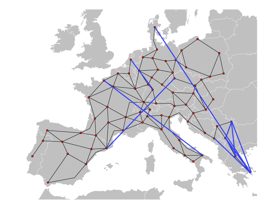
Figure 1: Best 10 HVDC line placements (in blue) according to the controllability Gramian trace metric.

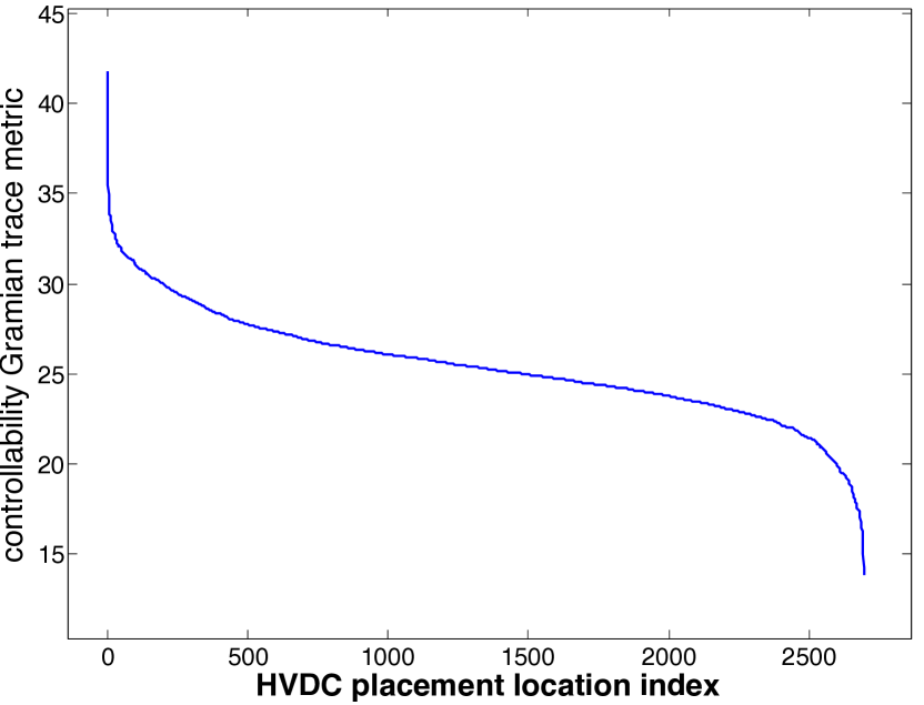
Figure 2: Distribution of the controllability Gramian trace metric.

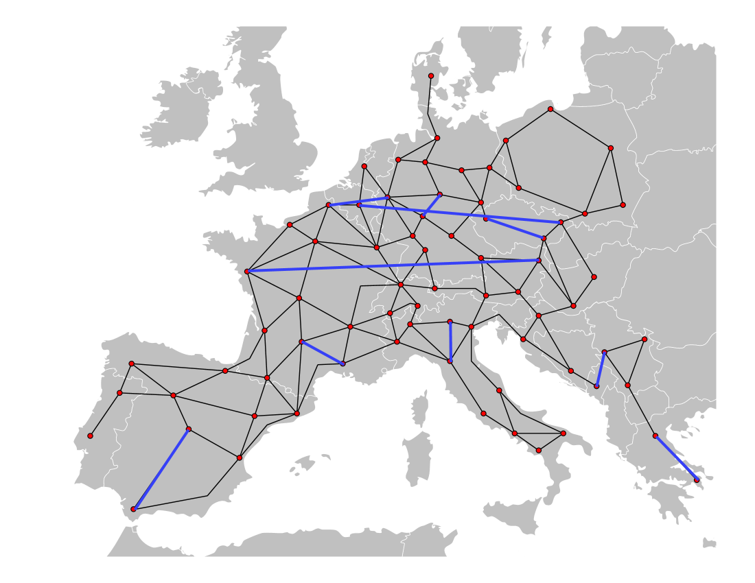
Figure 3: Best 10 HVDC line placements according to the controllability Gramian trace metric, weighted for frequency dynamics.

V Conclusions and Outlook

We have considered optimal actuator and sensor placement problems in complex dynamical networks. These problems are in general difficult combinatorial optimization problems; however, we have shown that an important class of metrics related to the controllability and observability Gramians yield modular set functions and are therefore efficiently globally optimized. We also defined the Average Energy Controllability Centrality measure, which assigns an importance value to each node in a dynamical network based on its ability to move the system around the state space with a low-energy time-varying control input. The results were illustrated via placement of power electronic actuators in a model of the European power grid.

There are many open problems involving the structure of combinatorial optimization problems in the optimal placement of sensors and actuators in complex networks. What other linear system controllability or observability metrics have exploitable combinatorial structure, e.g., modularity or submodularity? Further results have been obtained in [3]. Our ongoing work is exploring other case studies in power networks, biological networks, social networks, and discretized models of infinite-dimensional systems. Finally, more complicated systems (e.g. constrained, nonlinear, hybrid, etc.) require a full reachability analysis in general, which does not scale well, but one could explore how efficient methods could be used to obtain approximate metrics in these types of systems.

References

- [1] R.H. Bartels and GW Stewart. Solution of the matrix equation ax+ xb= c [f4]. Communications of the ACM, 15(9):820–826, 1972.
- [2] F.M. Callier and C.A. Desoer. Linear system theory. 1991.
- [3] F. Cortesi, T.H. Summers, and J. Lygeros. Submodularity of energy related controllability metrics. In submitted to the IEEE Conference on Decision and Control, 2014.
- [4] A. Fuchs and M. Morari. Grid stabilization through vsc-hvdc using wide area measurements. In IEEE PowerTech Conference, Trondheim, Norway, 2011.
- [5] A. Fuchs and M. Morari. Actuator performance evaluation using lmis for optimal hvdc placement. In European Control Conference, Zurich, Switzerland, 2013.
- [6] A. Fuchs and M. Morari. Placement of hvdc links for power grid stabilization during transients. In IEEE PowerTech Conference, Grenoble, France, 2013.
- [7] S. Fujishige. Submodular functions and optimization, volume 58. Elsevier Science Limited, 2005.
- [8] S.J. Hammarling. Numerical solution of the stable, non-negative definite lyapunov equation lyapunov equation. IMA Journal of Numerical Analysis, 2(3):303–323, 1982.
- [9] T. Hasse. Anforderung an eine durch Erneuerbare Energien geprägeigen Energieversorgung - Untersuchung des Regelverhaltens von Kraftwerken und Verbundnetzen. PhD thesis, University of Rostock, 2006.
- [10] A. Hassibi, J. How, and S. Boyd. Low-authority controller design via convex optimization. AIAA Journal of Guidance, Control, and Dynamics, 22(6):862–872, 1999.
- [11] T. Kailath. Linear systems, volume 1. Prentice-Hall Englewood Cliffs, NJ, 1980.
- [12] R. Kalman. On the general theory of control systems. IRE Transactions on Automatic Control, 4(3):110–110, 1959.
- [13] R.E. Kalman. Contributions to the theory of optimal control. Boletin de la Sociedad Matematica Mexicana, 5(1):102–119, 1960.
- [14] P. Kundur. Power system stability and control. McGraw-Hill, Inc., 1993.
- [15] C.T. Lin. Structural controllability. IEEE Transactions onAutomatic Control, 19(3):201–208, 1974.
- [16] Y.Y. Liu, J.J. Slotine, and A.L. Barabási. Controllability of complex networks. Nature, 473(7346):167–173, 2011.
- [17] L. Lovász. Submodular functions and convexity. Mathematical programming: the state of the art, pages 235–257, 1983.
- [18] F.J. Müller and A. Schuppert. Few inputs can reprogram biological networks. Nature, 478(7369):E4–E4, 2011.
- [19] T. Nepusz and T. Vicsek. Controlling edge dynamics in complex networks. Nature Physics, 8(7):568–573, 2012.
- [20] I. Rajapakse, M. Groudine, and M. Mesbahi. Dynamics and control of state-dependent networks for probing genomic organization. Proceedings of the National Academy of Sciences, 108(42):17257–17262, 2011.
- [21] Y. Tang, H. Gao, W. Zou, and J. Kurths. Identifying controlling nodes in neuronal networks in different scales. PloS one, 7(7):e41375, 2012.
- [22] M. Van De Wal and B. De Jager. A review of methods for input/output selection. Automatica, 37(4):487–510, 2001.
- [23] W.-X. Wang, X. Ni, Y.-C. Lai, and C. Grebogi. Optimizing controllability of complex networks by minimum structural perturbations. Physical Review E, 85(2):026115, 2012.
- [24] T. Yang, G. Huijun, J. Kurths, and J. Fang. Evolutionary pinning control and its application in uav coordination. Industrial Informatics, IEEE Transactions on, 8(4):828–838, 2012.