Stability of mode-locked kinks in the ac driven and damped sine-Gordon lattice

Abstract

Kink dynamics in the underdamped and strongly discrete sine-Gordon lattice that is driven by the oscillating force is studied. The investigation is focused mostly on the properties of the mode-locked states in the overband case, when the driving frequency lies above the linear band. With the help of Floquet theory it is demonstrated that the destabilizing of the mode-locked state happens either through the Hopf bifurcation or through the tangential bifurcation. It is also observed that in the overband case the standing mode-locked kink state maintains its stability for the bias amplitudes that are by the order of magnitude larger than the amplitudes in the low-frequency case.

Keywords: Nonlinear lattice dynamics, Josephson junction arrays, discrete sine-Gordon equation, kinks, fluxons, mode-locking, depinning, Floquet theory, Hopf bifurcation, tangential bifurcation, dynamical chaos.

1 Main Abbreviations

$\circ$ SG: Sine-Gordon	$\circ$ DSG: Discrete sine-Gordon
$\circ$ FK: Frenkel-Kontorova	$\circ$ PN: Peierls-Nabarro
$\circ$ JJ: Josephson junctions	$\circ$ JJA: Josephson junction arrays

2 Introduction

The discrete sine-Gordon (DSG) equation, also known as the Frenkel-Kontorova (FK) model, is ubiquitous in condensed matter physics fm96ap ; bk98pr . It has a wide range of applications in the dislocation theory fk38pzs , weak superconductivity wzso96pd ; u98pd and magnetism ms91adp . Among the intensively discussed problems for the DSG dynamics the problem of the topological soliton (fluxon) response to the ac (time-periodic) bias, remains to be important. This interest is caused in particular by the number of technological applications based on the Josephson junction arrays (JJAs), which are successively modelled by the DSG equation. Properties of the small ac-biased Josephson junctions have been extensively studied both experimentally (starting from the pioneering papers of Shapiro s63prl ) and theoretically (with the focus on the phase-locking k81japI and chaotic regimes k81japII ; k96rpp ). In particular, the rf-biased Josephson junctions have been used as a voltage standard k96rpp ; volts .

It is well-known pk84pd that contrary to the continuous sine-Gordon (SG) equation the DSG equation is non-integrable, and, moreover, it does not possess moving kink solutions. The ac-driven DSG lattice has two independent sources of non-integrability: the external drive (bias) and the discreteness. Interplay of these two sources has led to a number of interesting effects: mode-locking to the frequency of the external drive mfmfs97prb and kink mobility bm91prb ; fm99jpc (including its experimental detection in periodically modulated Josephson junctions um01prb ), various regimes of the dynamical chaos mfmfs97prb ; z12pre , biharmonically driven discrete kink ratchet zs06pre ; z12pre to name a few. However, these studies have been performed mostly in the adiabatic, subband (the driving frequency lies in the gap of the linear spectrum) or resonant (the driving frequency lies in the linear band) cases. The high-frequency limit when the driving frequency exceeds the linear wave frequency by several orders of magnitude has been studied in Refs. g-jk92pla ; kg-js92prb . In these papers the inversion of the ground state that is based on the Kapitza pendulum effect has been reported. The intermediate overband case when the bias frequency exceeds the linear wave frequency, but remains approximately of the same order of magnitude, requires a special attention. This frequency range is the natural bridge between the cases, studied in the papers, mentioned above. The dynamics of topological solitary waves (kinks), especially their linear stability in the intermediately high-frequency regime is the main aim of this paper.

The paper is organized as follows. The model, the equations of motion and the usage of the Floquet method for the linear stability studies are described in the next section. In the Section 4 we present the main properties of the standing kinks in the driven DSG lattice. The discussion and the main conclusions are given in the last Section.

3 The model and equations of motion

3.1 The DSG equation

The periodically driven and damped discrete sine-Gordon (DSG) equation is introduced in a dimensionless form as follows:

$$\ddot{\phi}_{n}-\kappa\Delta\phi_{n}+\sin\phi_{n}+\alpha\dot{\phi}_{n}+A\cos(\omega t)=0,~{}n=\overline{1,N}~{}.$$ (1)

Here $\Delta\phi_{n}\equiv\phi_{n+1}-2\phi_{n}+\phi_{n-1}$ is the discrete Laplacian and the dot represents the time differentiation. The physical meaning of the field variable $\phi_{n}$ depends on the underlying physical system. In the dislocation theory it stands for the particle displacement from its equilibrium position. In the JJ theory barone82 $\phi_{n}$ corresponds to the phase difference of the wave functions at the $n$th junction .

Only the periodic boundary conditions

$$\phi_{n+N}(t)=\phi_{n}(t)+2\pi Q,~{}{\dot{\phi}}_{n+N}(t)={\dot{\phi}}_{n}(t),$$ (2)

which correspond to the circular JJAs, are to be considered. The topological charge $Q$ is an integer constant that stands for the net number of kinks trapped in the lattice. Further on only we will study only the case of one kink ($Q=1$). The experiments with annular JJAs have been performed for typical lengths $N\sim 8-30$ (see Refs. wzso96pd ; u98pd ; baufz00prl ). In the following, we consider the case of an array (lattice) with $N=30$.

The dispersion law for the linear excitations (phonons) reads

$$\omega_{L}(q)=\sqrt{1+4\kappa~{}\sin^{2}\frac{q}{2}}~{}.$$ (3)

Due to finiteness of the array, the wavenumber $q\in[0,2\pi)$ attains only the discrete set of values $q_{m}=2\pi m/N$, $m=\pm 1,\ldots,\pm N$.

The regular kinks, mode-locked to the frequency of the external bias correspond to the limit cycles of Eq. (1). On these orbits, the average kink velocity is expressed as $\langle v\rangle=k\omega/(2\pi l)$, where the winding numbers $k$ and $l$ are integer. Thus, the kink travels $k$ sites during the time $lT=2\pi l/\omega$, so that, except for a shift in space, its profile is completely reproduced after this time interval (in the pendulum analogy, this orbit corresponds to $k$ full rotations of the pendulum during $l$ periods of the external drive).

3.2 Linear stability and the Floquet theory

In this article our main focus will be on the kinks locked to the external drive. In order to understand better their properties, we will focus on their linear stability. The fluxon periodic orbit is computed by finding zeroes of the map

$${\hat{\cal I}_{kl}}(T){\bf X}={\bf X},$$ (4)

where the vector ${\bf X}$ consists of the dynamical variables $\{\phi_{n},{\dot{\phi}}_{n}\}_{n=1}^{N}$. The operator ${\hat{\cal I}}_{kl}$ stands for the integration of the equations of motion (1) during the time $lT$ and afterwards the shift of the final solution by $k$ sites forward if $k<0$ or backward if $k>0$. The case $k=0$ corresponds to the fluxon pinned to a lattice site.

A fixed point of the map (4) is a mode-locked solution $\{\phi_{n}^{(0)}(t),{\dot{\phi}}_{n}^{(0)}(t)\}_{n=1}^{N}$ which reproduces itself after the time $lT$ with the space shift by $k$ lattice sites backward or forward. Next, we substitute the expansion

$$\phi_{n}(t)=\phi_{n}^{(0)}(t)+\varepsilon_{n}(t)~{},$$ (5)

into Eq. (1). For the case of standing kink ($k=0$) after keeping only the linear terms, we obtain the following set of linear ODEs with periodic coefficients:

$${\ddot{\varepsilon}}_{n}=-\alpha{\dot{\varepsilon}}_{n}+\kappa\Delta\varepsilon_{n}-\cos[\phi_{n}^{(0)}(t)]\varepsilon_{n}~{},~{}~{}n=1,2,\ldots,N.$$ (6)

The map

$$\left[\begin{array}[]{c}\vec{\varepsilon}(lT)\\ {\dot{\vec{\varepsilon}}}(lT)\end{array}\right]={\hat{M}}(T)\left[\begin{array}[]{c}\vec{\varepsilon}(0)\\ {\dot{\vec{\varepsilon}}}(0)\end{array}\right]$$ (7)

is constructed from the solutions of the system (6). It relates the small perturbations ${\vec{\varepsilon}}(t)=\{\varepsilon_{n}(t)\}_{n=1}^{N}$ at the time moments $t=0$ and $t=lT$. The $2N\times 2N$ Floquet (monodromy) matrix $\hat{M}$ contains all the necessary information about the linear stability of the system. If this matrix has at least one eigenvalue with $|\Lambda_{n}|>1$ ($n=1,2,\ldots,2N$), then the system is unstable. If for all eigenvalues $|\Lambda_{n}|\leq 1$, the system is stable. It is well-known via89 that these eigenvalues come in quadruples, so that if $\Lambda_{n}$ is an eigenvalue, then $\Lambda_{n}^{*}$, $R/\Lambda_{n}$ and $R/\Lambda_{n}^{*}$ (here $R=e^{-l\alpha\pi/\omega}$, see, for example, Refs. mffzp01pre ; mfmf01pre ) are also eigenvalues. Thus, the Floquet multipliers lie either on the circle of the radius $R$ (will be referred to as a $R$-circle throughout the paper) or may depart from it after collisions. The notable difference of the ac-driven case from the dc-driven (autonomous) case is the absence of the degeneration with respect to time shifts, which manifests itself in the absence of the eigenvalue $\Lambda=1$ sm97no .

Collision of the Floquet eigenvalues on the real axis signals the tangential (saddle-node) bifurcation if it happens at $\arg\Lambda=0$ or the period-doubling bifurcation if $\arg\Lambda=\pi$. Eigenvalue collision away from the real axis means that the Hopf bifurcation is taking place.

4 Kinks in the high-frequency driven DSG equation

In this paper, we plan to compute the mode-locked limit cycle that corresponds to the standing kink and to path-follow it while a control parameter is changed until the cycle becomes unstable or completely disappears. By monitoring the Floquet eigenvalues $\Lambda_{n}$ one can obtain the information about the underlying bifurcations and, consequently, about the unlocking process.

4.1 The numerical scheme

The scheme of the numerical studies can be described in the following way. As a starting iteration in the anti-continuum limit ($\kappa\equiv 0$) we consider the kink state that can be described by the following coding sequence

$$\{\underbrace{00\cdots 00}_{n=1,\ldots,N_{0}},\underbrace{2\pi\cdots 2\pi}_{n={N_{0}+1,\ldots,N}}\}~{}.$$ (8)

This means that we start with the kink which is centered between the $N_{0}$th and $N_{0}+1$th sites. In should be noted that due to the translational invariance the position of the kink center (defined by $N_{0}$) does not influence on the kink properties. The above choice of the coding sequence is defined by the well-known (see bk98pr ; pk84pd ) fact that such configuration, sometimes referred as a bond-centered kink, is stable for the DSG equation, in contrary to the site-centered kinks which are unstable. Then the initially stable (in the $\kappa=0$ limit) mode-locked state is continued numerically. For the numerical computation of the fixed point of Eq. (4) we use the Newton-Raphson iterative method. With this method it is possible to compute numerically the respective mode-locked limit cycle for the given period $lT$ with a desired computer precision. For details one might consult Ref. fw98pr , Chapter 6.1. The advantage of this approach is that not only attractors, but also repellers, can be computed. Also, wrong conclusions which can be made due to sensitivity to initial conditions can be avoided. Once the fixed point of (4) is computed, $\phi_{n}^{(0)}$ is plugged into Eqs. (6) and the Floquet matrix is computed and diagonalized with the standard numerical methods.

4.2 The existence diagram

It is well known that discreteness causes kink pinning to the lattice pk84pd . The kink in a lattice can be approximately described as a particle that moves in the spatially periodic potential (the PN potential) with the period that coincides with the lattice spacing. If the bias amplitude is weak enough, the kink will oscillate around the minima of the PN potential with the bias period. In other words, the kink oscillations are locked to the external drive. If the amplitude (or, alternatively, the coupling) is increased till some critical value, the external drive becomes strong enough to unlock the kink and to destroy the mode-locked state. Intuitively, it is not hard to understand that on the parameter plane $(\kappa,A)$ one can draw a curve $A_{c}=A_{c}(\kappa)$ that marks the loss of stability of a stable mode-locked standing kink. Suppose $\kappa$ is fixed and the mode-locked state is continued while the amplitude $A$ is increased until this state loses stability at $A=A_{c}$. At $A>A_{c}$, depending on the type of the destabilizing bifurcation and on the system parameters, different dynamical regimes can take place such as diffusively moving kinks, mode-locked moving kinks, quasiperiodic kinks, another standing mode-locked kink states with the different shape or even the chaotic dynamics of the whole array (when individual kinks cannot be identified). The latter case corresponds to the non-existing area and will not be discussed in this paper. The nature of the kink dynamics in the non-pinned area also strongly depends on the driving frequency $\omega$.

The existence diagrams on the $(\kappa,A)$ plane for the different values of $\omega$ are shown in Fig. 1. The critical dependence $A_{c}(\kappa)$ is defined by the first bifurcation that makes the mode-locked standing kink unstable.

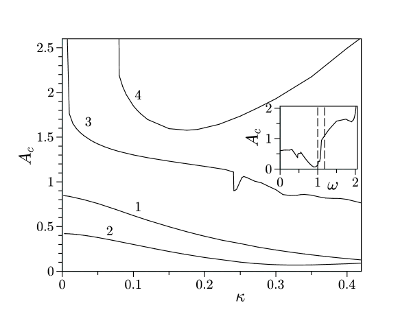
Figure 1: Existence diagram of standing mode-locked kinks for $\alpha=0.1$, $\omega=0.25$ (curve $1$), $\omega=0.7$ (curve $2$), $\omega=1.3$ (curve $3$) and $\omega=2$ (curve $4$). The inset shows the $A_{c}(\omega)$ at $\kappa=0.1$, the dashed vertical bars mark the edges of the linear band, $\omega_{L}(0)$ and $\omega_{L}(\pi)$.

In the case of subband [$0<\omega<\omega_{L}(q)$] frequencies the dependence $A_{c}(\kappa)$ is almost monotonic (see the curves $1-2$ in Fig. 1) with the two well-defined limiting cases. In the limit $\kappa\to\infty$, the effects of discreteness disappear, thus $A_{c}$ should decrease. On the other hand, the decrease of $\kappa$ means that the PN barrier becomes stronger and thus a larger amplitude is necessary to overcome it. As a result, $A_{c}$ increases when $\kappa\to 0$. The exit from the pinning area [below the curve $A_{c}(\kappa)$] can lead to different scenarios depending on the direction of the exit. The issue of discrete kink unlocking (depinning) in the DSG lattice driven by the subband frequencies has been studied in Refs. mfmfs97prb ; z12pre . In Fig. 2a the kink dynamics just above the $A_{c}$ value at $\kappa=0.1$ and $\omega=1.3>\omega_{L}(q)$ is shown. For these parameters the first destabilizing bifurcation takes place at $A_{c}\simeq 1.301145$, while the driving amplitude in Fig. 2a corresponds to the slightly larger value $A=1.3012$. It can be clearly observed that initially the kink stays pinned, but at $t\sim 5000$ it unlocks and begins to move chaotically. At this point we should remark that at $A<A_{c}$ the staning mode-locked kink is not the unique solution. Typically, the non-uniqueness is manifested by the existence of hysteresis loops in the neighbourhood of $A_{c}$ (for the subband case see Ref. mfmfs97prb ) . This situation is demonstrated in Fig. 2b-c. After crossing the critical value $A_{c}$ the driving amplitude is decreased back, and the chaotic moving solution is followed to the values $A<A_{c}$ (Fig. 2b) until it falls back to the mode-locked state as shown in Fig. 2c. The hysteresis loop appears to be quite narrow, constituting less then $1\%$ of $A_{c}$. At $\omega=0.35$ a different scenario has been observed, when the stability loss at $A_{c}$ leads to the complete kink destruction and chaotic dynamics of the whole lattice. If this chaotic solution is followed while $A$ is decreased, it does not return to the mode-locked kink state. Instead, at some $A_{*}<A_{c}$ the system falls back to the complex mode-locked state that includes the kink and one or several breathers, placed at the different lattice sites.

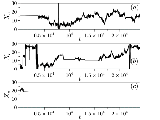
Figure 2: Time evolution of the kink center of mass $X_{c}=(4\pi)^{-1}\sum_{n=1}^{N}n(\phi_{n+1}-\phi_{n-1})$ at $\alpha=0.1$, $\omega=1.3$, $\kappa=0.1$, and $A=1.3012$ (a), $A=1.3$ (b) and $A=1.295$ (c).

The dependence on the driving frequency $A_{c}=A_{c}(\omega)$ is non-monotonic (see the inset in Fig. 1). The main resonance with the linear band can be clearly identified with the minimum at $\omega\simeq\omega_{L}(0)\equiv 1$. In this frequency range a linear wave around the kink can be excited at a rather small driving amplitude. Two significantly shallow minima at $\omega\simeq 0.5$ and $\omega\simeq 2$ appear due to the subharmonic half-frequency resonance and the resonance with the double frequency of the linear spectrum, respectively.

The case of overband frequencies [lying above the linear band, $\omega>\omega_{L}(q)$] is not well studied yet. Let us now focus on the curves $3-4$ in the Fig. 1. It should be noted that they are not monotonous, and, in addition they show sharp growth at $\kappa\to 0$. In order to understand this behaviour we study the Floquet spectrum and the nature of the destabilizing bifurcations.

4.3 Floquet spectrum and the destabilizing bifurcations

In the subband (low-frequency) case the stability loss leads to the unlocking of the standing kink. Typically it takes place through the tangential bifurcation mfmfs97prb which leads to the disappearance of the mode-locked state. After this bifurcation the kink starts to move in a chaotic way. More precisely, its regime belongs to the type-I intermittency. If the coupling is weak enough, the instability may lead to the destruction of the kink state and to chaotic motion of the whole lattice. In the neighbourhood of the main resonance $\omega\simeq 1$ the first destabilizing bifurcation is also tangential and it takes place at rather small values of the amplitude. It is caused by the resonance with the linear band and transforms the spatially monotonic standing kink into the standing kink with the oscillating background. Further increase of $A$ leads to the second destabilizing bifurcation after which the kink undergoes either depinning transition or destruction.

The case with $\omega=1.3$ that corresponds to the curve $3$ in the Fig. 1, can be considered either as overband or as a resonant depending on the value of $\kappa$, which defines the upper edge $\omega_{L}(\pi)=\sqrt{1+4\kappa}$ of the linear spectrum (3). Evolution of the Floquet spectrum for this case for the values of $\kappa=0.1$ and $\kappa=0.25$ is shown in Fig. 3. In the first case ($\kappa=0.1$) the bias frequency lies above the linear spectrum. In the anticontinuum limit, all the eigenvalues sit in one point and with the growth of $\kappa$ they separate, forming two distinct groups: the modes associated with the linear spectrum and the internal mode(s). The linear band extends with $\kappa$ according to the dispersion law (3), while the localized eigenmode is distinctly detached from the linear band, as can be clearly seen in Figs. 3a,c.

The destabilizing bifurcation takes place at $A\simeq 1.31$ and it can be clearly seen from the Fig. 3a that this is a Hopf bifurcation in which the localized mode [for the respective eigenvector shape see the inset in the panel (a)] is involved.

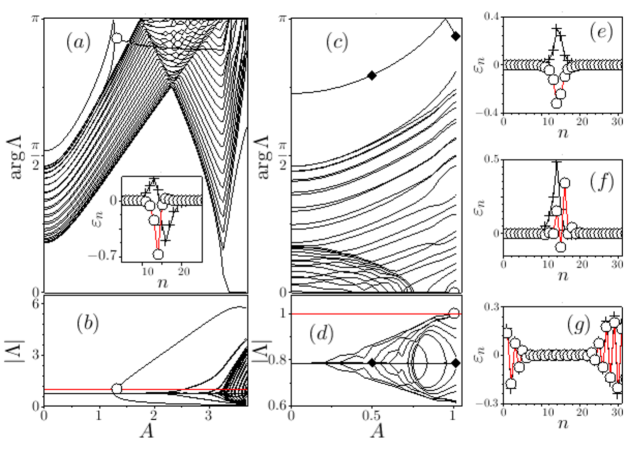
Figure 3: Phases and moduli of the Floquet multipliers as a function of the bias amplitude for $\omega=1.3$, $\kappa=0.1$ (a-b) and $\kappa=0.25$ (c-d). The inset in the panel (a) shows the unstable eigenvector at $A=1.31$. The dashed horizontal line in the panels (b) and (d) corresponds to the radius of the unit circle. The unstable eigenvalues are marked by $\circ$. Panels (e) and (f) show the shape of the localized eigenvector at $A=0.5$ and $A=1.015$, respectively. The respective eigenvalues are marked by $\blacklozenge$. Panel (g) shows the unstable eigenvector at $A=1.008$. In panels (e)-(g) $+$ corresponds to $\mbox{Re}\epsilon_{n}$ and $\circ$ corresponds to $\mbox{Im}\epsilon_{n}$. The rest of the parameters is the same as in Fig. 1.

Stability loss in this case causes the kink to unlock and to start moving chaotically along the lattice.

A different bifurcation scenario is observed when $\kappa=0.25$ (Figs. 3c-d). Now the resonance with the linear spectrum occurs and the destabilizing eigenvector is delocalized as shown in the Fig. 3g. Obviously it is associated with the linear spectrum. Indeed, one can clearly observe multiple collisions of the eigenvalues from the linear band on the positive side of real axis. These collisions are represented as “bubbles” in the $|\Lambda_{n}(A)|$ dependences Fig. 3d. One of these “bubbles” expands beyond the value $|\Lambda_{n}|=1$ at $A=1.008$ and causes the instability of the mode-locked state. The further small increase of the driving amplitude (to the value $A=1.095$) brings the kink to the regime of chaotic diffusion. The localized eigenvalue (Fig. 3e-f) stays distinctly detached from the linear band.

The resonance with the linear waves explains the small dip and some oscillations in the $A_{c}(\kappa)$ dependence (curve 3 in the Fig. 1). In the intervals $\kappa\in[0.241,0.253]$ and $\kappa\in[0.33,0.335]$ the first destabilizing bifurcation is the tangential (due to the resonance with the linear waves) and the Hopf bifurcation occurs later, while everywhere outside this interval it is the Hopf bifurcation which comes first. This tangential bifurcation occurs at slightly smaller values of $A$, therefore the respective interval on the $\kappa$ axis is marked by the small dip. We remind that due to the finiteness of the lattice the linear spectrum is discrete and the external ac bias resonates with the particular cavity modes. That is why the tangential bifurcation takes place not for all $\kappa\geq(\omega^{2}-1)/4$, but in the certain intervals of $\kappa$. After the tangential bifurcation the kink shape changes as it becomes surrounded by the non-decaying phonon tail.

Now we increase the bias frequency up to the value $\omega=2$. The behaviour of the Floquet multipliers as the bias amplitude is increased is shown in Fig. 4. Similarly to the previous case of $\omega=1.3$ the Hopf bifurcation, driven by the spatially localized perturbation (see Fig. 4c) makes the standing kink unstable. The instability leads to the appearance of a small localized mode on the top of the kink. The whole lattice is no longer in the mode-locked state but in the quasiperiodic, although the kink remains pinned. Further increase of $A$ leads to the second Hopf bifurcation at $A\simeq 5.25$ that restores the mode-locked standing kink state. Inside this interval the dynamic is quasiperiodic and no dynamical chaos has been detected. It appears that this Hopf bifurcation can be controlled by changing the system parameters. In particular, this can be done by varying the coupling constant $\kappa$, the bias frequency $\omega$ or the damping constant $\alpha$. After the Hopf bifurcation a number of tangential bifurcations take place at the much larger values of $A$. Some of them are destabilizing and some are not. Before discussing them we turn our attention on the control of the first (Hopf) bifurcation.

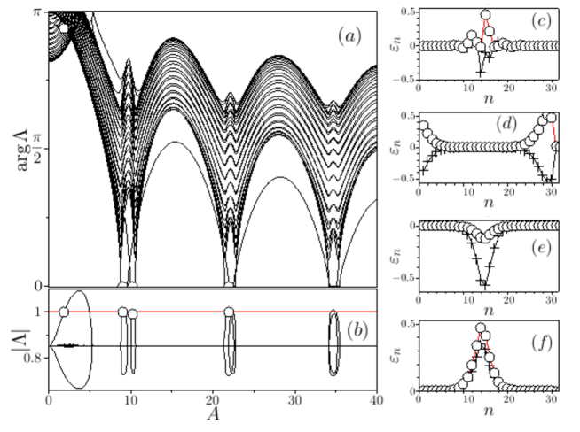
Figure 4: Phases (a) and moduli (b) of the Floquet multipliers as a function of the bias amplitude for $\kappa=0.1$, $\omega=2$ and $\alpha=0.1$. The dashed horizontal line in the panel (b) corresponds to the radius of the unit circle. The unstable eigenvectors [$\mbox{Re}\varepsilon_{n}$ ($+$) and $\mbox{Im}\varepsilon_{n}$ ($\circ$)] are shown in the panels (c) ($A=1.85$), (d) ($A=9$), (e) ($A=10.25$) and (f) ($A=22$). The respective eigenvalues are marked by $\circ$ in the panel (a).

In the Fig. 5 we show how the moduli of the Floquet eigenvalues evolve with the increase of $A$ for the different parameter values. The first case, shown in the Fig. 5a corresponds to the same frequency $\omega=2$, but the coupling is reduced to $\kappa=0.05$. As a result, the bubble associated with the destabilizing Hopf bifurcation is significantly reduced, and, more importantly, the collision of the respective Floquet eigenvalues does not lead to the instability, because these eigenvalues remain inside the unit circle. We have monitored the intermediate cases $\kappa=0.07,0.08,0.09$ and have observed the gradual increase of the bubble with the growth of $\kappa$ within this interval. Now we can explain the sharp growth of the $A_{c}(\kappa)$ dependence when $\kappa$ is decreased (see Fig. 1). It happens because the Hopf bifurcation does not longer lead to the kink instability, and the first destabilizing bifurcation is the tangential bifurcation. Similar control of the destabilizing bifurcation can be performed by increasing the damping parameter, which decreases $R$ and removes the instability. Interestingly, the increase of $\omega$ also reduces the Hopf bifurcation, and can completely remove it. This is demonstrated in the Figs. 5b-c, where the $|\Lambda_{n}(A)|$ is plotted for $\omega=2.1$ and $\omega=2.5$. In the case $\omega=2.1$ the “bubble” stays inside the unit circe, while in the case $\omega=2.5$ it is almost unnoticeable.

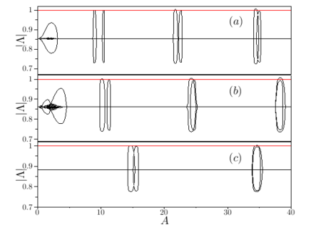
Figure 5: Moduli of the Floquet multipliers as a function of the bias amplitude for $\kappa=0.05$, $\omega=2$ (a); $\kappa=0.1$, $\omega=2.1$ and $\kappa=0.1$, $\omega=2.5$ (c). The dashed horizontal line marks the radius of the unit circle.

Another interesting observation that comes from Figs. 3-5 is the possibility of the standing kink existence for the rather large bias values that exceed the values of $A_{c}$ in the subband case by the order of magnitude. Indeed, if one forgets the first Hopf bifurcation (which can be controlled by the proper parameter choice anyway), the existence interval of the standing kink solution stretches along the $A$-axis interrupted only by narrow intervals where the Floquet multipliers exit the unit circle or approach it. These intervals are represented by the typical “bubbles” in the $|\Lambda_{n}(A)|$ dependencies in the Fig. 4b and in the Fig. 5. The amplitude of these bubbles can also be controlled by the increase of $\alpha$ so that the instability can be removed. These underlying bifurcations are the tangential ones and the respective unstable perturbation in the phase space is driven by the $U$-shaped eigenvector, as shown in Fig. 4d. It means that the instability develops in the following way: the core of the kink stays unchanged, while the tails tend to become deformed. The second bifurcation, on the contrary, causes the deformation in the kink core. In the Fig. 6 the change of the kink profiles with the growth of $A$ is shown. At $A=5$ the kink profile remains very much as for the usual strongly discrete kink. Further increase of $A$ leads to the broadening of the kink core and to the small deformation away from the core. Note that these deformations in the tail are actually caused by the instabilities, described in the previous paragraph. More precisely, they are associated with the tangential bifurcation at $A\sim 9$ and the instability direction, illustrated in Fig. 4d, prescribes exactly the same: the tail deformation. As the amplitude increased further, the deformation in the tails grows and the core straightens up. As a result, the kink restores its strongly localized shape, but now it is centered between the sites $N-1$ and $N$ (shown by $\blacklozenge$ in Fig. 6). Also, the field variable has been increased by $2\pi$. Further increase of the amplitude repeats the deformation scenario: in the neighbourhood of the second set of tangential bifurcations (around $A\sim 22-23.5$) the tails deform and the core straightens up. Finally the kink re-emerges in as a strongly localized excitation with its center placed between the sites $n=15$ and $n=16$.

Figure 6: Kink profiles for the case shown in Fig. 4 and for the different ac bias amplitudes: $A=5$ ($+$), $A=9$ ($\times$), $A=10$ ($\oplus$), $A=12$ ($\blacklozenge$), $A=20$ ($\diamond$), $A=22$ ($\Delta$), $A=23.5$ ($\nabla$) and $A=28$ ($\circ$). Solid lines are used as guides for an eye.

Note that the initially at $A=0$ the kink position was between the sites $n=14$ and $n=15$. The solution has been followed up to $A\simeq 50$ and such a transformation has been observed once again. Thus, the increase of the bias amplitude causes a sequence of the kink shape transformations that are driven by the tangential bifurcations and that shift the kink by $N/2$ sitels along the lattice. Here we have reached the high-frequency limit, described in Ref. g-jk92pla where the fast-oscillating drive effectively makes (after the averaging over the fast variables) the sine-term in the DSG equation to look like $J_{0}\left(A/[\omega\sqrt{\omega^{2}+\alpha^{2}}]\right)\sin\phi_{n}$ in the limit $\omega\gg 1$, and where $J_{0}$ is the Bessel function. As a result, depending on the driving amplitude the stable ground may become unstable, and back again, perfectly explaining the intermediate structures which have flat plateau at $\phi_{n}\sim\pi$ [$A=10$ ($\oplus$)] or at $\phi_{n}\sim 3\pi$ [$A=23.5$ ($\nabla$)] in Fig. 6.

5 Discussion and conclusions

To summarize, we have studied the kink stability in the ac-driven and damped sine-Gordon lattice. We have focused mainly on the overband regime where the bias frequency lies above the upper edge of the linear spectrum.

We have shown that the mode-locked high-frequency driven standing kink is much more stable with respect to the external ac drive comparing to the low-frequency driven kink. The critical bias amplitude at which the mode-locked state loses its stability may be several times larger in the high-frequency case comparing to the low-frequency case. For example, for the coupling $\kappa=0.1$ we have $A_{c}\simeq 0.62$ for $\omega=0.25$ and $A_{c}\simeq 1.85$ for $\omega=2$. For $\kappa=0.05$ the difference is even more drastic: $A_{c}\simeq 0.84$ ($\omega=0.25$) against $A_{c}\simeq 8.89$ ($\omega=2$). The instability of the mode-locked state is driven in the different frequency regime by the different bifurcations.

In the low-frequency case it is the tangential bifurcation, associated with the internal mode, while in the high-frequency case it is either Hopf bifurcation, associated again with the internal mode, or the tangential bifurcation, associated with the tail deformation. When the lattice is driven slowly, it is much easier to drive it away from the mode-locked state because different parts of the kink react in the different way to the perturbation: the kink may be depinned or even destroyed if the coupling is very small. Crossing the critical line $A_{c}(\kappa)$ in the low-frequency regime will almost probably lead either to the chaotic kink diffusion or to the complete kink destruction. The instability scenario in the high-frequency case is different. The Hopf bifurcation transforms the mode-locked periodic kink state into the quasiperiodic but still standing one with the small distortion in the core. Further increase of the driving amplitude may unlock the kink and it begins to travel chaotically along the lattice. If one takes even higher driving frequency and trace again the mode-locked states while the bias amplitude is increased, such an quasiperiodic state will not turn into the chaotic diffusive regime, but instead will be transformed back into the mode-locked state. Thus, the Hopf bifurcation can be controlled by the proper damping and/or frequency choice and the instability can be arrested.

Another interesting result is the kink structural deformation, driven by the tangential bifurcation at very large amplitudes ($A\gtrsim 10$). Here we reach the high-frequency limit, studied in Refs. g-jk92pla ; kg-js92prb where the ground state of the chain alternates between the $\phi=\pi$ and $\phi=2\pi$. We would like to note that the DSG lattice in the above-mentioned papers has been studied at $\kappa\geq 4$ and $\omega\sim 10-100$ what can be considered as a high-frequency driven weakly discrete case, while in this article we deal with the strongly discrete lattices at $\kappa<1$ and in the frequency range that exceeds the linear frequencies insignificantly: $\omega\sim 2$.

References

- (1) L. M. Floría and J. J. Mazo, Adv. Phys. 45, 505 (1996).
- (2) O. M. Braun and Y. S. Kivshar, Phys. Rep. 306, 2 (1998).
- (3) Ya. Frenkel and T. Kontorova, Phys. Z. Sowietunion 13, 1 (1938).
- (4) S. Watanabe, H. S. J. van der Zant, S. H. Strogatz, and T. P. Orlando, Physica D 97, 429 (1996).
- (5) A. V. Ustinov, Physica D 123, 315 (1998).
- (6) H.-J. Mikeska and M. Steiner, Advances in Physics 40, 191 (1991).
- (7) S. Shapiro, Phys. Rev. Lett. 11, 80 (1963); S. Shapiro, A. R. Janus, and S. Holly, Rev. Mod. Phys. 36, 223 (1964).
- (8) R. L. Kautz, J. Appl. Phys. 52, 3528 (1981).
- (9) R. L. Kautz, J. Appl. Phys. 52, 6241 (1981); E. Ben-Jacob, Y. Braiman, R. Shainsky and Y. Imry, Appl. Phys. Lett. 38, 822 (1981); R. L. Kautz and R. Monaco, J. Appl. Phys. 57, 875 (1985);
- (10) R. L. Kautz, Rep. Prog. Phys. 59 (1996) 935.
- (11) M. T. Levinsen, R. Y. Chiao, M. J. Feldman and B. A. Tucker, Appl. Phys. Lett. 31, 776 (1977); R. L. Kautz, Appl. Phys. Lett. 36, 386 (1980).
- (12) M. Peyrard and M. D. Kruskal, Physica D 14, 88 (1984).
- (13) P. J. Martínez, F. Falo, J. Mazo, L. M. Floría, and A. Sánchez, Phys. Rev. B 56, 87 (1997).
- (14) L. L. Bonilla and B. A. Malomed, Phys. Rev. B 43, 11539 (1991).
- (15) G. Filatrella and B. A. Malomed, J. Phys.: Condens. Matter 11, 7103 (1999).
- (16) A. V. Ustinov and B. A. Malomed, Phys. Rev. B 64, 020302(R) (2001).
- (17) Y. Zolotaryuk and M. Salerno, Phys. Rev. E 73, 066621 (2006).
- (18) Y. Zolotaryuk, Phys. Rev. E 86, 026604 (2012).
- (19) N. Grønbech-Jensen and Y. S. Kivshar, Phys. Lett. A 171 (1992) 338.
- (20) Y. S. Kivshar, N. Grønbech-Jensen, and M. R. Samuelsen, Phys. Rev. B 45 (1993) 7789.
- (21) A. Barone, G. Paterno: Physics and Applications of the Josephson Effect, (Wiley, New York 1982).
- (22) P. Binder, D. Abraimov, A. V. Ustinov, S. Flach, and Y. Zolotaryuk, Phys. Rev. Lett. 84, 745 (2000).
- (23) V. I. Arnol’d, Mathematical Methods of Classical Mechanics (Springer, Berlin, 1989).
- (24) A. E. Miroshnichenko, S. Flach, M. V. Fistul, Y. Zolotaryuk, and J. B. Page, Phys. Rev. E 64, 066601 (2001).
- (25) J. L. Marín, F. Falo, P. Martínez, and L. M. Floría, Phys. Rev. E 63, 066603 (2001).
- (26) J. A. Sepulchre and R. S. MacKay, Nonlinearity 10, 679 (1997).
- (27) C. Baesens, S. Kim, and R. Mackay, Physica D Nonlinear Phenomena 113, 242 (1998).
- (28) S. Flach and C. R. Willis, Phys. Rep. 295, 182 (1998).