Abstract

Here we present two explicit counterexamples to the widely spread beliefs about an exclusive role of bimodality as the first order phase transition signal. On the basis of an exactly solvable statistical model generalizing the statistical multifragmentation model we demonstrate that the bimodal distributions can naturally appear both in infinite and in finite systems without a phase transition. In the first counterexample a bimodal distribution appears in an infinite system at the supercritical temperatures due to the negative values of the surface tension coefficient. In the second counterexample we explicitly demonstrate that a bimodal fragment distribution appears in a finite volume analog of a gaseous phase. In contrast to the statistical multifragmentation model, the developed statistical model corresponds to the compressible nuclear liquid with the tricritical endpoint located at one third of the normal nuclear density. The suggested parameterization of the liquid phase equation of state is consistent with the L. van Hove axioms of statistical mechanics and it does not lead to an appearance of the non-monotonic isotherms in the macroscopic mixed phase region which are typical for the classical models of the Van der Waals type. Peculiarly, such a way to account for the nuclear liquid compressibility automatically leads to an appearance of an additional state that in many respects resembles the physical antinuclear matter.

Key words: Statistical multifragmentation model, surface tension, compressible nuclear liquid, bimodality
PACS: 21.65.+f, 24.10.Pa, 25.70.Pq

1 Introduction

During the last decade the studies of the nuclear liquid-gas phase transition (PT) stimulated both theoretical and experimental interest to the bimodal distributions [1, 2, 3, 4, 5, 6, 7, 8]. Moreover, some theoretical arguments [1, 2, 3, 4], although obtained approximately, which relate the bimodal distribution of a certain order parameter and the location of the Yang-Lee zeros [9] in a complex fugacity plane became so popular that nowadays the bimodality is considered as a signal of the first order PT in finite systems, whereas the opposite opinions [10, 11, 12] are, in fact, ignored. The scheme connecting the bimodality and the Yang-Lee zeros [2, 4] is so abstract and general that the authors failed even to discuss the physical origin of the bimodal distribution. However, in our opinion this is a crucial point, since in the nuclear physics experiments at intermediate energies one cannot get the purely statistical distributions of any observable because the process of collision is a dynamical one and, hence, we cannot account for or extract the dynamical fluctuations of the initial conditions, the fluctuations of the number of participating nucleons, or possible instabilities occurring during the course of the system expansion and/or freeze out. Moreover, it is not evident that the observed bimodal distributions are not generated by the imposed experimental cuts.

The authors of these theoretical scheme [2, 3, 4] implicitly assumed that the measured distributions and the corresponding partition function of the dynamically evolving system produced in the nuclear reaction generated by the recipe of [2, 3, 4] do, indeed, correspond to the equilibrium partition function of the original physical system. This assumption, however, cannot be justified without having a complete dynamical model which correctly describes the whole evolution of the system. Moreover, even, if one is able to completely account for the whole dynamical aspects of the system evolution and, thus, is able to extract the purely statistical distributions, then there is no guaranty that the suggested theoretical scheme [2, 3, 4] will work without any additional conditions. For example, it is absolutely unclear what one should do, if the extracted statistical distributions do not correspond to the statistical ensemble of the physical system under consideration? For the macroscopic systems we do not have such a problem, since for the vast majority of systems all the statistical ensembles are equivalent and, hence, one can easily change them and choose the appropriate one. This, however, is not the case for finite or even small systems which are studied in the nuclear physics experiments.

The second typical mistake of Ref. [1, 2, 3, 4] and the similar schemes [13, 14] is that the authors of such schemes identify each local maximum of the bimodal distribution with a pure phase. Even in a famous textbook of T. Hill on thermodynamics of small systems [13] such an assumption is a corner stone of his treatment of PTs in finite systems. In contrast to the authors of the scheme [2, 3, 4] Hill justified his assumption on bimodality by stating that due to the fact that an interface between two pure phases ’costs’ some additional energy, the probability of their coexisting in a finite system is less than for each of pure phases. We, however, should remind that the assumption on the pure phases existence in small system is taken from the examples of infinite systems, whereas for finite systems such an assumption cannot be justified. Moreover, the examples of the constrained statistical multifragmentation model (CSMM) [15] and the gas of hadron bags model [12] which are exactly solved for finite systems and which allow one to rigorously define analogs of phases for finite grand canonical systems, show that, in contrast, to assumptions of Refs. [1, 2, 4, 13, 14], in finite systems the pure liquid phase cannot exist at finite pressures. Instead, it can appear only as a part of mixed phase which is represented by even number of thermodynamically metastable states [15, 12].

Therefore, here we would like to give some counterexamples to the claims of Refs. [1, 2, 4, 13] by considering the exact analytical solutions of the CSMM in the thermodynamic limit and for the finite volumes which lead to the bimodal fragment distributions inside of the cross-over region and inside of the gaseous phase. For this purpose we consider the CSMM with two new elements. The first of them is a more realistic equation of state for the liquid phase which, in contrast to the original SMM formulation [16, 17, 18], is a compressible one. The second important element of the present model is a more realistic parameterization for the temperature dependence of surface tension that is based on the exact analytical solution of the partition function of surface deformations [19, 20]. Besides these two new elements allow us to study a realistic phase diagram of the CSMM both for finite systems and for infinite system.

The work is organized as follows. In sect. 2 we describe the new parameterization of the CSMM liquid phase pressure which repairs the two main pitfalls of the original SMM and allows one to consider the compressible liquid which has the tricritical endpoint at the phase diagram at the one third of the normal nuclear density. It is also shown that the bimodal fragment size distributions may appear at the supercritical temperatures due to negative values of the surface tension coefficient and without any PT. Sect. 3 is devoted to the analysis of finite systems using the exact solution of CSMM. In this section we demonstrate that the bimodal fragment size distribution is generated within the finite volume analog of the gaseous phase. Our conclusions are formulated in sect. 4.

2 CSMM with compressible nuclear liquid in thermodynamic limit

The general solution of the CSMM partition function formulated in the grand canonical variables of volume $V$, temperature $T$ and baryonic chemical potential $\mu$ is given by [12, 15, 21, 22]

$${\cal Z}(V,T,\mu)~{}=\sum_{\{\lambda_{n}\}}e^{\textstyle\lambda_{n}\,V}{\textstyle\left[1-\frac{\partial{\cal F}(V,\lambda_{n})}{\partial\lambda_{n}}\right]^{-1}}\,,$$ (1)

where the set of $\lambda_{n}$ $(n=0,1,2,3,..)$ are all the complex roots of the equation

$$\lambda_{n}~{}=~{}{\cal F}(V,\lambda_{n})\,,$$ (2)

ordered as $Re(\lambda_{n})>Re(\lambda_{n+1})$ and $Im(\lambda_{0})=0$. The function ${\cal F}(V,\lambda)$ is defined as

$${\cal F}(V,\lambda)=\left(\frac{mT}{2\pi}\right)^{\frac{3}{2}}z_{1}~{}\exp\left\{\frac{\mu-\lambda Tb}{T}\right\}+\sum_{k=2}^{K(V)}\phi_{k}(T)\exp\left\{\frac{(p_{l}(T,\mu)-\lambda T)bk}{T}\right\}\,.$$ (3)

Here $m\simeq 940$ MeV is a nucleon mass, $z_{1}=4$ is an internal partition (the degeneracy factor) of nucleons, $b=1/\rho_{0}$ is the eigen volume of one nucleon in a vacuum ($\rho_{0}\simeq 0.17$ fm³ is the normal nuclear density at $T=0$ and zero pressure). The reduced distribution function of the $k$-nucleon fragment in (3) is defined as

$$\phi_{k>1}(T)\equiv\left(\frac{mT}{2\pi}\right)^{\frac{3}{2}}k^{-\tau}\,\exp\left[-\frac{\sigma(T)~{}k^{\varsigma}}{T}\right]\,,$$ (4)

where $\tau\simeq 1.825$ [18] is the Fisher topological exponent and $\sigma(T)$ is the $T$-dependent surface tension coefficient. Usually, the constant, parameterizing the dimension of surface in terms of the volume is $\varsigma=\frac{2}{3}$, but in this work we would like to give the results for a wide range of its values, namely for $0<\varsigma<1$.

In (3) the exponents $\exp(-\lambda bk)$ ($k=1,2,3,...$) appear due to the hard-core repulsion between the nuclear fragments [15, 17, 21], while $p_{l}(T,\mu)$ is the pressure of the liquid phase [21, 22]. As one can see from (3) the nucleons are treated differently compared to larger fragments: they do not have the surface free energy and all the bulk free energy characteristics except for the baryonic charge which are encoded in the liquid phase pressure $p_{l}(T,\mu)$ (see later). In principle, the fragments with the mass below ten nucleon masses can be parameterized in a similar way [16, 21], but for the sake of simplicity we treat in this way the nucleons only. Such a treatment does not affect the properties of the phase diagram in the thermodynamic limit, since exclusion of any finite number of light fragments from the sums in (3) does not affect the PT existence and its order [15, 17, 21].

Note also that the complex free energy density $-T{\cal F}(V,\lambda)$ [15] of the present model contains neither the Coulomb energy nor the asymmetry energy. This assumption is similar to Refs. [17, 18, 23] and allows us to study the nuclear matter properties in the thermodynamic limit. However, in contrast to Refs. [17, 18, 23], the model free energy density $-T{\cal F}(V,\lambda)$ in (3) contains the liquid phase pressure that can be chosen in a general form and the size of maximal fragment $K(V)$ that can be a desired function of the system volume $V$. However, in this section we consider the thermodynamic limit only, i.e. for $V\rightarrow\infty$ it follows $K(V)\rightarrow\infty$. Then the treatment of the model is essentially simplified, since Eq. (2) can have only two kinds of solutions [17, 15, 21], either the gaseous pole $p_{g}(T,\mu)=T\lambda_{0}(T,\mu)$ for ${\cal F}(V,\lambda_{0}-0)<\infty$ or the liquid essential singularity $p_{l}(T,\mu)=T\lambda_{0}(T,\mu)$ for ${\cal F}(V,\lambda_{0}-0)\rightarrow\infty$. The mathematical reason why only the rightmost solution $\lambda_{0}(T,\mu)=\max\{Re(\lambda_{n})\}$ of Eq. (2) defines the system pressure is evident from Eq. (1): in the limit $V\rightarrow\infty$ all the solutions of (2) other than the rightmost one are exponentially suppressed.

In the thermodynamic limit the model has a PT, when there occurs a change of the rightmost solution type , i.e. when the gaseous pole is changed by the liquid essential singularity or vice versa. The PT line $\mu=\mu_{c}(T)$ is a solution of the equation of ‘colliding singularities’ $p_{g}(T,\mu)=p_{l}(T,\mu)$ [17, 15, 21], which is just the Gibbs criterion of phase equilibrium. The properties of a PT are defined only by the liquid phase pressure $p_{l}(T,\mu)$ and by the temperature dependence of surface tension $\sigma(T)$, since the value of Fisher exponent $\tau=1.825$ is fixed by the values of the critical indices of ordinary liquids [18] and by the experimental findings [24, 25].

In order to avoid the incompressibility of the nuclear liquid we suggest to consider the following simplest parameterization of its pressure

$$p_{l}=\frac{W(T)+\mu+a_{2}(\mu-\mu_{0})^{2}+a_{4}(\mu-\mu_{0})^{4}}{b}\,.$$ (5)

Note that the above way to account for the nuclear liquid compressibility is fully consistent with the L. van Hove axioms of statistical mechanics [26, 27] and, hence, it does not lead to an appearance of the non-monotonic isotherms in the mixed phase region which are typical for the mean-field models. In [22] the liquid phase pressure was parameterized as a second order polynomial in the baryonic chemical potential. In our mind Eq. (5) is more favorable, since it allows one to easily get a correct value for the nuclear incompressibility factor for a normal nuclear liquid. In Eq. (5) $W(T)=W_{0}+\frac{T^{2}}{W_{0}}$ denotes the usual temperature dependent binding energy per nucleon [16, 17] with $W_{0}=16$ MeV and the constants $\mu_{0}$, $a_{2}$ and $a_{4}>0$. In principle, these constants should be fixed in the way to reproduce the properties of normal nuclear matter, i.e. at vanishing temperature $T=0$ and normal nuclear density $\rho=\rho_{0}$ the liquid pressure must be zero

$$W_{0}+\mu_{c}(0)+a_{2}(\mu_{c}(0)-\mu_{0})^{2}+a_{4}(\mu_{c}(0)-\mu_{0})^{4}=0\,,$$ (6)

where $\mu_{c}(0)$ is the baryonic chemical potential at the PT line taken at $T=0$. Finding the particle density of the liquid as $\rho_{l}=\frac{\partial p_{l}}{\partial\mu}$

$$\rho_{l}(\mu)=\frac{1+2\,a_{2}\tilde{\mu}+4\,a_{4}\,\tilde{\mu}^{3}}{b}\,,\quad{\rm with}\quad\tilde{\mu}=\mu-\mu_{0}\,,$$ (7)

one can get the equation for $\mu_{c}(0)$, i.e. from $\rho_{l}(\mu_{c}(0))=\rho_{0}$ it follows $2\,a_{2}\tilde{\mu}(0)+4\,a_{4}\,\tilde{\mu}(0)^{3}=0$, where the shifted chemical potential $\tilde{\mu}(0)$ is defined as $\tilde{\mu}(0)\equiv\mu_{c}(0)-\mu_{0}$. Usually, an additional requirement to fix the nuclear liquid model parameters is related to the incompressibility factor of the normal nuclear matter [28] which is defined as

$$K_{0}\equiv 9\left(\frac{\partial p_{l}}{\partial\rho_{l}}\right)_{T=0}=\frac{9(1+2\,a_{2}\tilde{\mu}(0)+4\,a_{4}\,\tilde{\mu}(0)^{3})}{2\,a_{2}+12\,a_{4}\,\tilde{\mu}(0)^{2}}\,.$$ (8)

The present day experimental estimates for the incompressibility factor are $K_{0}^{exp}=230\pm 30$ MeV [29, 30, 31, 32], but the models with the typical value $K_{0}=300-360$ MeV are also well known [28, 31]. For instance, the Skyrme force model SIII, which is able to successfully describe the experimental properties of many nuclei [31], has the value of the nuclear incompressibility factor $K_{0}=355$ MeV. Therefore, instead of describing exactly the present day values of the normal nuclear incompressibility factor and have many additional parameters, we prefer to keep the model as simple as possible, but to require that at the tricritical point the baryonic density is $\rho_{cep}=\rho_{0}/3$ which is typical for the liquid-gas PTs [33]. The latter generates the following equation for the shifted value of the baryonic chemical potential at the tricritical endpoint: $2\,a_{2}\tilde{\mu}_{cep}+4\,a_{4}\,\tilde{\mu}_{cep}^{3}=-\frac{2}{3}$, where $\tilde{\mu}_{cep}\equiv\mu_{cep}-\mu_{0}$.

Choosing $\mu_{0}=-W_{0}=-16$ MeV, we obtain $\tilde{\mu}(0)=0$ and, hence, the expressions (6) and (7) are essentially simplified, respectively, giving us $\rho_{l}(\mu_{c}(0))\equiv\rho_{0}$ and $K_{0}=\frac{9}{2\,a_{2}}$. Then, solving the phase equilibrium condition at the tricritical endpoint together with the condition on the baryonic density at this point, one can express both the coefficient $a_{4}$ and $\tilde{\mu}_{cep}$ in terms of $a_{2}$ and the pressure of gaseous phase $p_{g}(T_{cep},\mu_{cep})$ taken at this point. Thus, one can express $K_{0}$, $\rho_{l}(\mu_{c}(T_{cep}))$ and $a_{4}$ in terms of $a_{2}$ and $p_{g}(T_{cep},\mu_{cep})$. However, we found that for $K_{0}<350$ MeV the obtained values of the coefficient $a_{4}$ are negative which leads to an instability of nuclear liquid at very high baryonic densities. Therefore, in order to avoid these problems, we fixed $K_{0}=365$ MeV which leads to $a_{2}\simeq 1.233\cdot 10^{-2}$ MeV^-1 and $a_{4}\simeq 4.099\cdot 10^{-7}$ MeV^-3. Thus, the present model is able to repair the two major unrealistic features of the original SMM, namely, it provides one with a reasonable value for the nuclear liquid compressibility and with a physically motivated value for the baryonic density at the tricritical endpoint.

In addition to the new parameterization of the free energy of the $k$-nucleon fragment (3) we propose to consider a more general parameterization of the surface tension coefficient

$$\sigma(T)=\sigma_{0}\left|\frac{T_{cep}-T}{T_{cep}}\right|^{\zeta}{\rm sign}(T_{cep}-T)~{},$$ (9)

with $\zeta=const\geq 1$, $T_{cep}=18$ MeV and $\sigma_{0}=18$ MeV the SMM [16]. In contrast to the Fisher droplet model [34] and the usual SMM [16], the CSMM surface tension (9) is negative above the critical temperature $T_{cep}$. It is necessary to stress that there is nothing wrong or unphysical with the negative values of surface tension coefficient (9), since $\sigma(T)\,k^{\varsigma}$ in (4) is the surface free energy of the fragment of mean volume $b\,k$ and, hence, as any free energy, it contains the energy part $e_{surf}$ and the entropy part $s_{surf}$ multiplied by temperature $T$ [34]. Therefore, at low temperatures the energy part dominates and the surface free energy is positive, whereas at high temperatures the number of fragment configurations with large surface drastically increases and it exceeds the Boltzmann suppression and, hence, the surface free energy becomes negative since $s_{surf}>\frac{e_{surf}}{T}$. Because of this reason the negative values of the surface tension coefficient were recently employed in a variety of exactly solvable statistical models for the deconfinement PT [35, 36, 37, 38]. For the first time this fact was derived within the exactly solvable model for surface deformations of large physical clusters [19]. Very recently an important relation between the surface tension of large quark gluon bags and the string tension of two static color charges measured by the lattice QCD was derived [39]. Based on such a relation it was possible to conclude that at high temperatures the surface tension coefficient of quark gluon bags should be negative [39, 40].

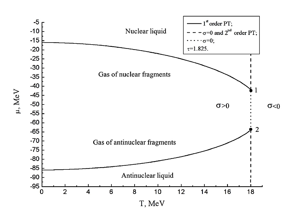
Figure 1: The phase diagram in $T-\mu$ plane. The first order PT occurs along the solid curves. Above the upper curve there exists the nuclear matter, while below the lower one there is an analog of the antinuclear matter. The vertical dashed lines show the second order PT and the black circles correspond to the tricritical endpoints marked by the digits 1 (nuclear matter) and 2 (antinuclear matter). A cross-over occurs along the dotted vertical line of the vanishing surface tension coefficient.

Furthermore, a thorough analysis of the temperature dependence of the surface tension coefficient in ordinary liquids [41, 42] shows not only that the surface tension coefficient approaches zero, but, in contrast to the widely spread beliefs, for many liquids the full $T$ derivative of $\sigma(T)$ does not vanish and remains finite at $T_{cep}$: $\frac{d~{}\sigma(T)}{d~{}T}<0$ [41]. Therefore, just the naive extension of these data to the temperatures above $T_{cep}$ would lead to negative values of surface tension coefficient at the supercritical temperatures. On the other hand, if one, as usually, believes that $\sigma\equiv 0$ for $T>T_{cep}$, then it is absolutely unclear what physical process can lead to simultaneous existence of the discontinuity of $\frac{d~{}\sigma}{d~{}T}$ at $T_{cep}$ and the smooth behavior of the pressure’s first and second derivatives at the cross-over. Finally, the negative values of the surface tension at supercritical temperatures is the only known physical reason which prevents the condensation of smaller droplets into a liquid phase and, thus, it terminates the first order PT existence and degenerates it into a cross-over at these temperatures. Therefore, we conclude that negative values of the surface tension coefficient at supercritical temperatures are also necessary for ordinary liquids although up to now this question has not been investigated.

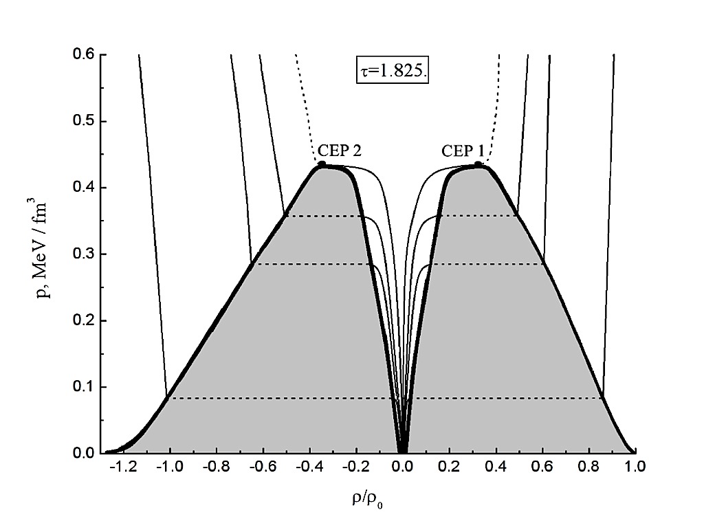
Figure 2: The phase diagram in $\rho-p$ plane. The grey areas show the mixed phases of the first order PTs. The isotherms are shown for $T=11,16,17,18$ MeV from bottom to top. Negative density values correspond to an ‘antimatter’. For the densities $|\rho/\rho_{0}|\geq 1/3$ at the isotherm $T=18$ MeV there exists the second order PT. The tricritical endpoints are marked by the digits 1 (nuclear matter) and 2 (antinuclear matter).

Similarly to the simplified SMM [17, 18], for $T<T_{cep}$ the present model has the nuclear liquid-gas PT of the first order. However, as one can see from Fig. 1 in this region of temperatures the model has two first order PTs. The meaning of the second PT curve can be understood from Fig. 2. At first glance a mathematical cause of an ‘antimatter’ appearance may look surprising since the gas pressure contains no fragments with negative baryonic charges. However, this is true for $\left|\frac{\tilde{\mu}}{T}\right|\ll 1$ only, while for $\left|\frac{\tilde{\mu}}{T}\right|\geq 1$ the main contribution in the liquid phase pressure $p_{l}$ in (5) is defined by the term $a_{4}\tilde{\mu}^{4}$ and, hence its derivative with respect to $\mu$ determines a sign of the baryonic charge density of both a liquid phase and a gas of nuclear fragments. The letter can be seen from the charge density expression for the gaseous phase. Indeed, finding the $\mu$ derivative of the gaseous phase pressure $p_{g}=T\lambda_{0}(T,\mu)$ from Eqs. (2) and Eqs. (3), one finds the baryonic charge density of the gaseous phase as

$$\rho_{g}=\frac{\rho_{0}\,\left(\frac{mT}{2\pi}\right)^{\frac{3}{2}}z_{1}~{}\exp\left\{\frac{\mu-\lambda Tb}{T}\right\}+\rho_{l}\,\sum_{k=2}^{\infty}\phi_{k}(T)\,k\,\exp\left\{\frac{(p_{l}(T,\mu)-p_{g}(T,\mu))bk}{T}\right\}}{1+\left(\frac{mT}{2\pi}\right)^{\frac{3}{2}}z_{1}~{}\exp\left\{\frac{\mu-\lambda Tb}{T}\right\}+\sum_{k=2}^{\infty}\phi_{k}(T)\,k\,\exp\left\{\frac{(p_{l}(T,\mu)-p_{g}(T,\mu))bk}{T}\right\}}\,.$$ (10)

From this expression one can see that, if the contribution of the nucleons (proportional to $z_{1}$) is small compared to the sum over other nuclear fragments, i.e. for $\left(\mu-b\,p_{l}(T,\mu)\right)/T<-1$, then the baryonic charge density of the gaseous phase is proportional to that one of liquid, i.e. ${\rm sign}\left[\rho_{g}\right]={\rm sign}\left[\rho_{l}\right]$. Of course, one should not take this additional solution as a physical antinuclear matter, since the gas pressure of the present model contains only the nuclear fragments with the charges $k=1,2,3,...$ that stay in front of the nonrelativistic value of the baryonic chemical potential $\mu$ and does not contain any terms with an opposite value of $\mu$. It is clear that in a relativistic treatment one would have the symmetry with respect to the charge conjugation $\mu_{rel}\leftrightarrow-\mu_{rel}$ for the relativistic baryonic chemical potential $\mu_{rel}\equiv m+\mu$. Nevertheless, it is a remarkable fact, that the simplest way to account for the nuclear liquid compressibility which is consistent with the L. van Hove axioms of statistical mechanics [26, 27] automatically leads to an appearance of an additional state that in many respects resembles the physical antinuclear matter.

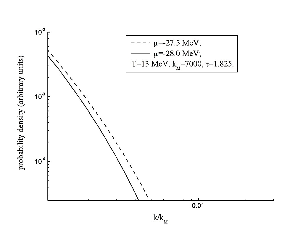
Figure 3: Fragment size distribution in the gaseous phase is shown for a fixed temperature $T=13$ MeV and two values of the baryonic chemical potential $\mu$. The number of nucleons in a fragment is $k$. The larger value of $\mu$ corresponds to the gaseous state at the phase boundary with the mixed phase. The calculations were made for the largest fragment of $K(V)=k_{M}=7000$ nucleons.

Also Eq. (10) clearly shows that at the phase equilibrium, i.e. for the same pressure, the baryonic densities of gaseous and liquid phases differ, if the sum staying both in numerator and in denominator of (10) is not divergent. This is possible, either for positive values of the surface tension coefficient $\sigma(T)>0$ and any positive value $\tau>0$ or, alternatively, for $\sigma(T)=0$ and $\tau>2$. In either of these two cases there is a first order PT. If, however, $\sigma(T)=0$ and $\tau\leq 2$, which is the case for the present model at $T=T_{cep}$, then for some values of the chemical potential one has $\rho_{g}(T_{cep},\mu_{cep})=\rho_{l}(T_{cep},\mu_{cep})$ and the sums in (10) diverge. Then at these points there exists a PT of higher order. The analysis of higher order derivatives of gaseous pressure made similarly to [35] shows that for $2\geq\tau>\frac{3}{2}$ at the critical endpoint of this model there exists a second order PT. In the present model a second order PT exists not only at the critical endpoints, but at the two lines in the $T-\mu$ plane along which the surface tension is zero (see the two vertical dashed lines in Fig. 1). Therefore, the both critical endpoints of the present model are the tricritical endpoints. This feature is similar to the simplified SMM [17, 18] and it is robust for $\tau=1.825$, whereas as one can see from Fig. 2 the second order PTs of this model are not located at the constant density as in the simplified SMM. Finally, for the supercritical temperatures the surface tension (9) is negative and, hence, the phase equilibrium is not possible in this case [17, 18, 21].

Now we would like to study the fragment size distribution in two regions of the phase diagram in order to elucidate the role of the negative surface tension coefficient. In order to demonstrate the pitfalls of the bimodal concept of Refs. [1, 2, 3, 4, 13] we study only the gaseous phase and the supercritical temperature region, where there is no PT by construction. As one can see from Fig. (3) in the gaseous phase, even at the boundary with the mixed phase, the size distribution is a monotonically decreasing function of the number of nucleons in a fragment $k$. The found distributions are very similar to those one shown in Fig. 5 of [43] for comparable temperatures. As one can see from Fig. 3 for small fragments the distribution is almost power-like one (notice the double logarithmic scale in Fig. 3), while for larger fragments the deviation from a pure power law is seen. No bimodal distribution is found in this case, although in actual simulations we used $K(V)=k_{M}=7000$ nucleons.

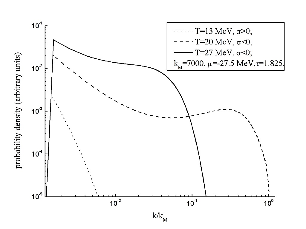
Figure 4: Fragment size distribution in the gaseous phase is shown for a fixed baryonic chemical potential $\mu=-27.5$ MeV and three values of the temperature $T$. The legend is similar to Fig. 3. The dotted curve in this figure corresponds to the solid curve in Fig. 3.

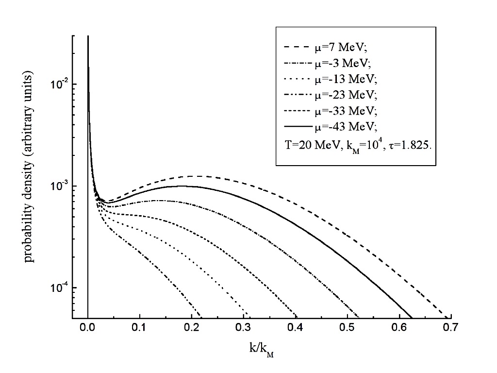
Figure 5: Fragment size distribution in the gaseous phase is shown for a fixed temperature $T=20$ MeV and several values of the baryonic chemical potential $\mu$. The legend is similar to Fig. 3. The principal difference with the distributions shown in Fig. 3 is the presence of negative surface tension coefficient. Note that the shown fragment size distributions demonstrate a nonmonotonic dependence on the baryonic chemical potential.

However, for the supercritical temperatures one finds the typical bimodal fragment distribution for a variety of temperatures and chemical potentials as one can see from Figs. 4 and 5. It is necessary to stress that by construction at this region the phase equilibrium is impossible due to negative surface tension coefficient, but the fragment distribution is bimodal and it very closely resembles the weighted fragment size distributions found for the lattice gas model in [4] shown there in Fig. 5 and considered by the author of [4] as a clear PT signal in a finite system. The bimodal distributions of the present model consist of three elements: there is a sharp peak at low $k$ values, then at intermediate fragment sizes there exists a local minimum, while at large fragment sizes there is a wide maximum. A sharp peak reflects a fast increase of the probability density of dimers compared to the monomers (nucleons), since the latter do not have the binding free energy and the surface free energy and, hence, the monomers are significantly suppressed in this region of thermodynamic parameters. On the other hand it is clear that the tail of fragment distributions in Figs. 4 and 5 decreases due to the dominance of the bulk free energy and, hence, the whole structure at intermediate fragment sizes is due a competition between the surface free energy and two other contributions into the fragment free energy, i.e. the bulk one and the Fisher one.

Let us demonstrate now that the bimodal fragment size attenuation appears due to the negative value of the surface tension coefficient, i.e. for $\sigma(T)<0$. In the latter case the gaseous pressure exceeds that one of the liquid phase, i.e. the effective chemical potential $\nu\equiv(p_{l}(T,\mu)-p_{g}(T,\mu))\,b<0$ is negative [17, 21]. Then the unnormalized distribution of nuclear fragments with respect to the number of nucleons $k$

$$\omega(k)=\exp\left[-\frac{|\nu|}{T}\,k+\frac{|\sigma|}{T}k^{\varsigma}-\tau\ln k\,\right]\,,$$ (11)

has the local minimum at some value $k_{min}$ and the local maximum at $k_{max}>k_{min}$. This can be shown by inspecting the logarithmic derivative of $\omega(k)$ with respect to $k$. Thus, the extremum condition for such a derivative gives us

$$\left.\frac{\partial\ln\omega(k)}{\partial\,k}\right|_{k=k_{E}}=-\frac{|\nu|}{T}+\frac{|\sigma|}{T}\,\frac{\varsigma}{k^{1-\varsigma}_{E}}\,-\frac{\tau}{k_{E}}=0\quad\Rightarrow\quad k_{E}=\left[\frac{\varsigma\,|\sigma|}{|\nu|+\frac{\tau\,T}{k_{E}}}\right]^{\frac{1}{1-\varsigma}}\,,$$ (12)

where the extremum is reached for $k=k_{E}$. Let us show now that the expression for $k_{E}$ in (12) has two positive solutions. In the first case we assume that the Fisher term dominates over the bulk one, i.e. $|\nu|\ll\frac{\tau}{k_{E}}$, which may occur only for small values of $k_{E}$. Then neglecting the term $|\nu|$ in the above expression for $k_{E}$ one finds

$$k_{min}=k_{E}\simeq\left[\frac{\tau\,T}{\varsigma\,|\sigma|}\right]^{\frac{1}{\varsigma}}\,.$$ (13)

The analysis of the second derivative of $\ln\omega(k)$ with respect to $k$

$$\left.\frac{\partial^{2}\ln\omega(k)}{\partial\,k^{2}}\right|_{k=k_{min}}=-\varsigma(1-\varsigma)\,\frac{|\sigma|}{T\,k^{2-\varsigma}_{min}}\,+\frac{\tau}{k^{2}_{min}}=\frac{\varsigma\,\tau}{k^{2}_{min}}>0\,,$$ (14)

shows that this derivative is always positive, i.e. there is a local minimum, for $\varsigma>0$. Note that Eq. (13) allows one to roughly estimate the surface tension as $\sigma\simeq-\frac{\tau\,T}{\varsigma\,k_{min}^{\varsigma}}$, if the position of the local minim is known (for an exact expression see below).

In the opposite case, if the bulk free energy dominates over the Fisher term, i.e. for $|\nu|\gg\frac{\tau\,T}{k_{E}}$, which occurs only for large values of $k_{E}$, the solution for $k_{E}$ takes the form

$$k_{max}=k_{E}\simeq\left[\frac{\varsigma\,|\sigma|}{|\nu|}\right]^{\frac{1}{1-\varsigma}}\,,$$ (15)

and, therefore, the second derivative of $\ln\omega(k)$ with respect to $k$ can be written as

$$\left.\frac{\partial^{2}\ln\omega(k)}{\partial\,k^{2}}\right|_{k=k_{max}}=-\varsigma(1-\varsigma)\,\frac{|\sigma|}{T\,k^{2-\varsigma}_{max}}\,+\frac{\tau}{k^{2}_{max}}=-\frac{1}{k_{max}}\left[\frac{(1-\varsigma)\,|\nu|}{T}-\frac{\tau}{k_{max}}\right]\,.$$ (16)

Now it is clear that the second derivative (16) is negative for $|\nu|(1-\varsigma)>\frac{\tau\,T}{k_{max}}$. Note that the latter inequality cannot be fulfilled for $(1-\varsigma)\ll 1$ only, whereas for the typical SMM value $\varsigma\simeq\frac{2}{3}$ the inequality $|\nu|(1-\varsigma)>\frac{\tau\,T}{k_{max}}$ is obeyed due to adopted assumption $|\nu|\gg\frac{\tau\,T}{k_{max}}$. Thus, at $k\simeq k_{max}$ the fragment distribution (11) has a local maximum. The existence of the distribution with the saddle like shape that has both a local minimum and a local maximum which are clearly seen in Figs. 4 and 5.

In fact, if the positions of both local extrema are known, i.e. $k_{min}$ and $k_{max}$ are known, for instance, from the experiment, then for a given temperature $T$ one can exactly find both $\nu$ and $\sigma$. To demonstrate this, we introduce a new variable $x$

$$k_{E}^{\varsigma}\equiv\frac{\tau\,T}{\varsigma\,|\sigma|}(1+x)\,.$$ (17)

Then in terms of this variable the extremum condition (12) can written as

$$\frac{\tau\,T}{|\nu|}x=\left[\frac{\tau\,T}{\varsigma\,|\sigma|}(1+x)\right]^{\frac{1}{\varsigma}}\,.$$ (18)

since $k_{E}\equiv\frac{\tau\,T}{|\nu|}x$. Denoting the solutions of Eq. (18) as $x_{1}=\frac{|\nu|}{\tau\,T}\,k_{min}$ and $x_{2}=\frac{|\nu|}{\tau\,T}\,k_{max}\equiv R\,x_{1}$ and dividing expression (18) for $x=x_{2}$ by the same expression for $x=x_{1}$, one obtains the following equation for $x=x_{1}$

$$R=\left[\frac{1+R\,x_{1}}{1+x_{1}}\right]^{\frac{1}{\varsigma}}\quad\Rightarrow\quad x_{1}=\frac{R^{\varsigma}-1}{R-R^{\varsigma}}\,,\quad x_{2}=R\,\frac{R^{\varsigma}-1}{R-R^{\varsigma}}\,,$$ (19)

if the ratio $R\equiv\frac{x_{2}}{x_{1}}\equiv\frac{k_{max}}{k_{min}}$ is known from the fragment distribution. The above results allow us to explicitly find the effective chemical potential $\nu$ and the surface tension coefficient $\sigma$ as

$$|\nu|=\frac{\tau\,T}{k_{min}}\cdot\frac{R^{\varsigma}-1}{R-R^{\varsigma}}\,,\quad|\sigma|=\frac{\tau\,T}{\varsigma\,k_{min}^{\varsigma}}\cdot\left[1+\frac{|\nu|}{\tau\,T}\,k_{min}\right]=\frac{\tau\,T}{\varsigma\,k_{min}^{\varsigma}}\cdot\frac{R-1}{R-R^{\varsigma}}\,.$$ (20)

These expressions can be useful for the experimental data analysis.

From the above analysis it is evident that the bimodal distributions demonstrated in Figs. 4 and 5 have nothing to do with the PT existence, but appear due to the competition of the negative surface free energy with the positive free energy terms generated by the Fisher topological exponent and the bulk term, which, respectively, dominate at small and large values of fragment size. Thus, we give an explicit example to the widely spread belief [1, 2, 3, 4, 13] that a bimodal distribution of typical order parameter (size of fragment) is an exclusive signal of a first order PT in finite systems. Together with the authors of Refs. [10, 11, 12] we would like to stress that without studying the nature of the bimodal distributions one cannot claim that a PT is its only origin.

Furthermore, the existence of bimodal distributions without a PT completely breaks down the logic of T. Hill [13]. According to [13] the interface energy between two phases should essentially suppress the coexistence of two ‘pure’ phases, but the states at supercritical temperatures are, indeed, kind of the coexistence of two phases, but in an absence of a PT and, hence, without an explicit surface separating them.

3 Bimodal distributions at finite volumes

In this section we would like to thoroughly analyze the second typical mistake of the approaches [2, 3, 4, 13, 14] based on bimodality properties of a first order PT in finite systems. In these approaches it is implicitly assumed that, like in infinite systems, in finite systems there exist exactly two ‘pure’ phases and they correspond to two peaks in the bimodal distribution of the order parameter. The examples given in the preceding section correspond to the thermodynamic limit, although in actual simulations we used $7\cdot 10^{3}$ and $10^{4}$ particles. We found that further increase of the size of the largest fragment $K(V)$ in (3) generates the relative numerical errors below $10^{-8}$ compared to the results obtained in the thermodynamic limit. In this section, however, we consider smaller systems whose behavior is far from the thermodynamic limit.

In order to illustrate some of the results which are necessary for a discussion of bimodality in finite systems we introduce the real $R_{n}$ and imaginary $I_{n}$ parts of $\lambda_{n}=R_{n}+iI_{n}$ and consider Eq. (2) as a system of coupled transcendental equations

$$R_{n}=~{}\sum\limits_{k=1}^{K(V)}\phi_{k}(T)~{}\exp\left[\frac{Re(\nu_{n})\,k}{T}\right]\cos(I_{n}bk)\,,$$ (21)

$$I_{n}=-\sum\limits_{k=1}^{K(V)}\phi_{k}(T)~{}\exp\left[\frac{Re(\nu_{n})\,k}{T}\right]\sin(I_{n}bk)\,,$$ (22)

where for convenience we introduced the following set of the effective chemical potentials $\nu_{n}$

$$\nu_{n}\equiv\nu(\lambda_{n})=p_{l}(T,\mu)b-(R_{n}+iI_{n})b\,T\,,$$ (23)

and the reduced distribution for nucleons $\phi_{1}(T)=\left(\frac{mT}{2\pi}\right)^{\frac{3}{2}}z_{1}\exp((\mu-p_{l}(T,\mu)b)/T)$.

Consider the real root $(R_{0}>0,I_{0}=0)$, first. Similarly to the SMM [17], for $I_{n}=I_{0}=0$ the real root $R_{0}$ of the CSMM exists for any $T$ and $\mu$. Comparison of $R_{0}$ from (21) with the expression for vapor pressure of the analytical SMM solution [17] indicates that $TR_{0}$ is a constrained grand canonical pressure of the mixture of ideal gases with the chemical potential $\nu_{0}$. Let us show that that the gas singularity is always the rightmost one. First we assume that for the same set of $T,\mu$ and $V$ there exists a complex root $R_{n>0}$ which is the rightmost one compared to $R_{0}$, i.e. $R_{n>0}>R_{0}$ for $I_{n>0}\neq 0$. Then one immediately concludes that $Re(\nu_{n>0})<Re(\nu_{0})$, but in this case for $n>0$ one obtains

$$R_{n}=\sum\limits_{k=1}^{K(V)}\phi_{k}(T)\,{\textstyle\exp\left[\frac{Re(\nu_{n})\,k}{T}\right]\,\cos(I_{n}bk)}<\sum\limits_{k=1}^{K(V)}\phi_{k}(T)\,{\textstyle\exp\left[\frac{Re(\nu_{0})\,k}{T}\right]}=R_{0}\,,$$ (24)

i.e. we arrive at a contradiction with the original assumption.

Note, however, that assuming an opposite inequality $R_{n>0}<R_{0}$ for $I_{n>0}\neq 0$ and $I_{0}=0$, one cannot get a contradiction, since a counterpart of the inequality (24) cannot be established for $Re(\nu_{n>0})>Re(\nu_{0})$ due to the fact that for $I_{n>0}\neq 0$ some of the $k$-values in the sum in Eq. (22) unavoidably would generate the inequality $\cos(I_{n}bk)<1$. This means that the gas singularity is always the rightmost one. Such a fact plays a decisive role in a formulating the finite volume analogs of phases [15] and it will be exploited below as well.

Since Eq. (22) is not changed under the substitution $I_{n}\leftrightarrow-I_{n}$ then the complex roots of the system (21), (22) are coming in pairs only. This is an evident consequence of the fact that the grand canonical partition (1) must be real. Now it is also apparent that all the roots can be classified according to a descending order of their real parts.

A rigorous mathematical scheme to identify the analogs of phases in finite systems for the partitions (1)-(4) was worked out in [15, 12, 21]. It is based on the number of roots of the system (21), (22) for a given set of grand canonical variables $T,\mu$ and $V$. Thus, a single real solution $\lambda_{0}=R_{0}$ with $I_{0}=0$ of the system (21), (22) corresponds to a gaseous phase, since its pressure, indeed, looks like a pressure of a mixture of ideal gases with a single value of the effective baryonic chemical potential $\nu_{0}$ defined by (23). If the system (21), (22) has one real solution $\lambda_{0}$ and any natural number $n=1,2,3,...$ of complex conjugate pairs of roots $\lambda_{n\geq 1}$ then the corresponding partition (1) describes a mixture of a gaseous phase with a set of metastable states which are not in a true chemical equilibrium with the gas, since the real parts of their free energy $-TVR_{n>0}$ are larger than the corresponding value for the gaseous phase, i.e. $-TVR_{n>0}>-TVR_{0}$. The absence of a true chemical equilibrium between these metastable states and the gas is also seen from that the fact the real parts of their effective chemical potential $\nu_{n}$ of is larger than the value of the effective chemical potential of the gaseous phase $\nu_{0}$, i.e. $Re(\nu_{n>0})>\nu_{0}$. A finite system analog of a fluid phase corresponds to an infinite number of the complex roots of the system (21), (22), but it exists at infinite pressure only.

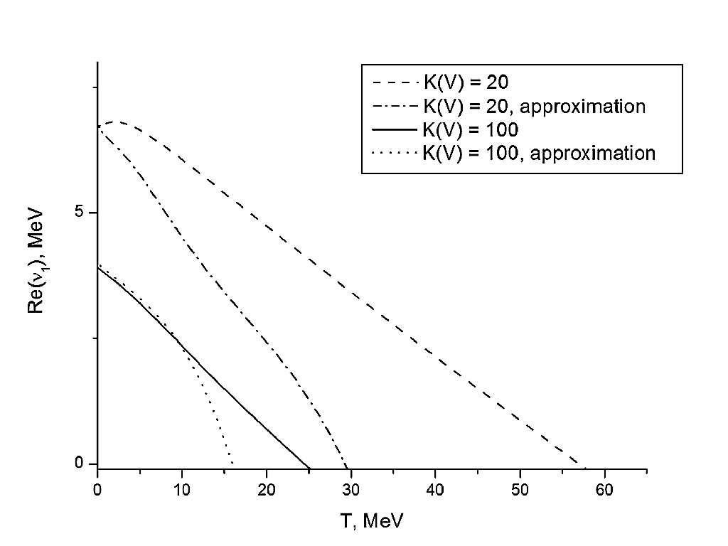
Figure 6: The finite volume analog of the phase diagram in $T-Re(\nu_{1})$ plane for given values of $K(V)=20$ (dashed curve) and $K(V)=100$ (solid curve). Below each of these phase boundaries there exists a gaseous phase only, but at and above each curve there are three or more solutions of the system (21), (22). These solutions describe the states that can be identified as a finite volume analog of a mixed phase. The additional curves correspond to the approximation (29).

Using this scheme, one can build up the finite system analog of the $T-\mu$ phase diagram. Indeed, the curve $Re(\nu_{1}(T))$ divides the temperature-chemical potential plane into three regions: for the region $Re(\nu_{n})<Re(\nu_{1}(T))$ there is only a single solution of the system (21), (22) which describes the gaseous phase, at the curve $Re(\nu_{n})=Re(\nu_{1}(T))$ there are exactly three roots of the system (21), (22) while above for $Re(\nu_{n})>Re(\nu_{1}(T))$ there are five or more roots of this system, which corresponds to a finite volume analog of mixed phase. Fig. 6 shows such a curve $Re(\nu_{1}(T))$. The principal difference with the thermodynamic limit discussed in the preceding section is that for finite volumes the effective chemical potential in the gaseous phase can be positive, i.e. for some temperatures one has $\nu_{0}>0$. Knowing the values of $Re(\nu_{1}(T))$ and $R_{1}(T)$, one can find the corresponding value of the liquid pressure, which, in its turn, allows one to determine the curve $\mu_{1}(T)$ from the liquid phase equation of state (5). Such curves $\mu_{1}(T)$ are shown in Fig. 7 for two values of the maximal fragment size $K(V)$. Comparing the $T-\mu$ phase diagrams of Fig. 7 with that ones shown in Fig. 1, one can see that for temperatures below $T_{cep}$ all the curves are quantitatively similar to each other even for a small system with $K(V)=20$. However, in contrast to the thermodynamic limit phase diagram of Fig. 1, for considered finite systems the curves $\mu_{1}(T)$ for the nuclear matter and ‘antinuclear’ matter are connected with each other at temperatures about $T_{cep}$.

It is necessary to stress that, in contrast to the infinite systems, the partial pressures $TR_{n}$ of the states $n=0,1,2,3,..$ that belong to the same grand canonical partition of a finite system (1) do not coincide with each other and, therefore, in contrast to the beliefs of the authors of [2, 3, 4, 13], the statistical weights of the gaseous phase $(n=0)$ and the states with $n\geq 1$ can be quite different. Moreover, although the state with $n=0$ is a gaseous phase, the states with $n\geq 1$ cannot be identified as a ‘pure’ liquid, since they have different partial pressures and different decay/formation times defined via the imaginary part of the free energy as $\tau_{n}\equiv\left[I_{n}bT\right]^{-1}$ [12, 15, 21]. Furthermore, in finite systems even the gaseous phase differs from that one existing in the thermodynamic limit, since, as one can see from Fig. 6, for finite volumes $V$ the effective chemical potential can be positive, i.e. $\nu_{0}>0$, and this case corresponds to entirely different distribution of fragments.

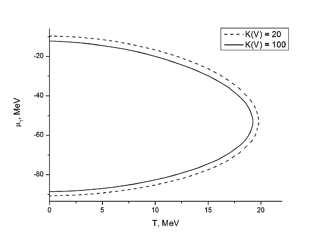
Figure 7: The image of the finite volume analog of the phase diagram $T-Re(\nu_{1})$ of Fig. 6 is shown in terms of the usual variables $T$ and $\mu$. Note that for finite $K(V)$ the solutions $\mu_{1}(T)$ do not exist for some temperatures $\max(T)>T_{cep}$ and, thus, the both phase equilibrium curves of Fig. 1 form a continuous phase diagram for a finite system.

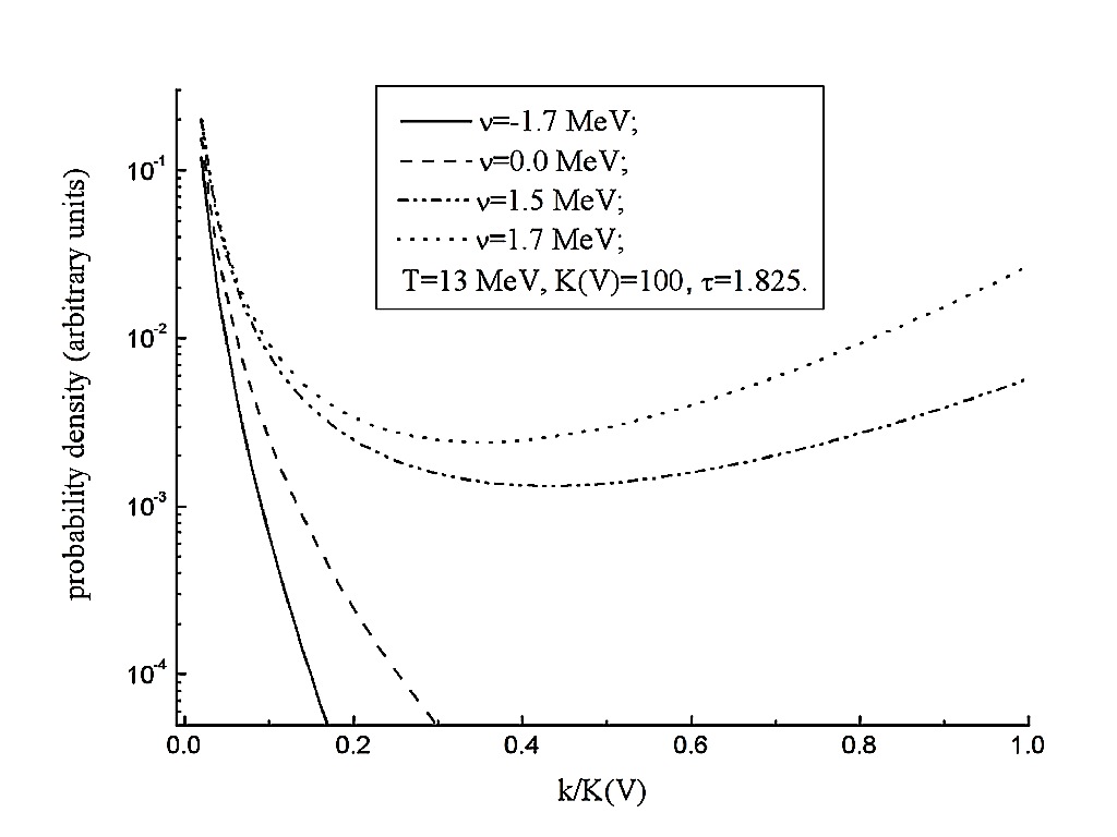
Figure 8: Typical fragment size distributions existing in a finite analog of gaseous phase are shown for a fixed temperature $T=13$ MeV and different value of the effective chemical potential $\nu_{0}$. For positive values of $\nu_{0}$ the fragment distribution has a bimodal like shape, although it is still a gas of all fragments. The maximal size of nuclear fragment is $K(V)=k_{M}=100$ nucleons.

Indeed, as one can see from Fig. 8 for positive values of the effective chemical potential $\nu_{0}$ the fragment size distributions in a finite analog of gaseous phase acquires a bimodal like shape without any PT. Existence of such distributions is another explicit counterexample against Hill belief [13] that the bimodal distributions can be used to unambiguously characterize a PT in finite systems.

Since an existence of the states with $\nu_{0}>0$ is of principal importance for this study, here we would like to demonstrate this fact analytically. For this purpose we consider the limit $Re(\nu_{n})\gg T$ for all $0<n<N0$ with $N\gg 1$. For instance, this is a typical situation for low temperatures $T$ or it can appear at high baryonic densities existing inside of a mixed phase. It is clear, that in this limit the leading contribution to the right hand side of (22) corresponds to the harmonic with $k=K(V)$, and, consequently, an exponentially large amplitude of this term can be only compensated by a vanishing value of $\sin\left(I_{n}\,bK(V)\right)$, i.e. $I_{n}\,bK=\pi n+\delta_{n}$ with $|\delta_{n}|\ll\pi$ (hereafter we will analyze only the branch $I_{n}>0$). Keeping the leading term on the right hand side of (22) and solving for $\delta_{n}$, one finds [15, 21, 22]

$$I_{n} \approx \frac{2\pi\,n+\delta_{n}}{K(V)\,b}\approx\frac{2\pi\,n}{K(V)\,b}\left[1-\frac{1}{K(V)\,b\,R_{n}}\right]\,,$$ (25)

$$\delta_{n} \approx -\frac{2\pi n}{K(V)\,b\,R_{n}}\,,$$ (26)

$$R_{n} \approx \phi_{K}(T)~{}\exp\left[\frac{Re(\nu_{n})\,K(V)}{T}\right]\,,$$ (27)

where the results are given for the branch of positive $R_{n}$ values.

Since for large volumes $V$ the negative values of $R_{n}$ cannot contribute to the grand canonical partition (1), here we analyze only values of $n$ which generate $R_{n}>0$. In this case substituting the reduced distribution (9) into Eq. (27) one obtains the leading terms for the partial pressure of $n$-th state

$$TR_{n} \approx p_{l}(T,\mu)-\frac{T}{b\,K(V)}\ln\left|\frac{R_{n}}{\phi_{K}(T)}\right|$$ (28)

$$\approx p_{l}(T,\mu)-\frac{\sigma(T)}{b\,[K(V)]^{1-\varsigma}}-T\left[\frac{\ln|\left(\frac{2\pi}{mT}\right)^{\frac{3}{2}}R_{n}|+\tau\ln K(V)}{b\,K(V)}\right]\,,$$

under the inequalities $Re(\nu)\gg T$ and $K(V)\gg 1$. This equation clearly shows that for $K(V)\gg 1$ and $\varsigma=\frac{2}{3}$ the $n$-th state corresponds to a finite droplet of a radius of $K(V)^{\frac{1}{3}}$ nucleon radii having a volume pressure of an infinite liquid droplet which is corrected by the Laplace surface pressure (the second term on the right hand side of (28)). In fact, such states correspond to a mixed phase dominated by a heaviest fragment. This is clearly seen from (28) at low temperatures. Indeed, for $T\rightarrow 0$ the left hand side of (28) and the last term on the right hand side of it vanish and we obtain that equations for all $R_{n>0}$ degenerate into the same expression $p_{l}(0,\mu_{1})-\frac{\sigma(0)}{b\,[K(V)]^{1-\varsigma}}\approx 0$, which is a condition of vanishing total pressure of the finite liquid drop, where the chemical potential $\mu_{1}$ corresponds to $R_{1}$. In other words, the vanishing total pressure of the $n$-th state is the mechanical stability condition of mixed phase, since at $T\rightarrow 0$ the gaseous phase pressure is zero. A few examples of $\mu_{1}(T)$ are depicted in Fig. 7.

Also Eq. (28) obviously demonstrates that in the thermodynamic limit $K(V)\rightarrow\infty$ an infinite number of metastable states with partial pressures $TR_{n>0}\rightarrow p_{l}(T,\mu)$ go to the real axis of the complex $\lambda$-plane, since in this limit $I_{n>0}\rightarrow 0$ in (25), and, hence, they form a pole of infinite order at $\lambda_{n>0}=p_{l}(T,\mu)/T$, i.e. they form an essential singularity of the isobaric partition function [12, 15, 21, 22] which, in contrast to a simple pole of a gaseous phase $\lambda_{0}=R_{0}$, describes a liquid phase.

From Eq. (28) one can get the effective chemical potentials $Re(\nu_{n>0})$ of these $n$-states as

$$Re(\nu_{n>0})\approx\frac{\sigma(T)}{[K(V)]^{1-\varsigma}}+T\left[\frac{\ln|\left(\frac{2\pi}{mT}\right)^{\frac{3}{2}}R_{n>0}|+\tau\ln K(V)}{K(V)}\right]\,,$$ (29)

from which one can immediately deduce that for low temperatures and for $K(V)\gg 1$ the real part of $\nu_{n>0}$ is solely defined by the sign of the surface tension coefficient, i.e. from $\sigma(T)>0$ it follows that $Re(\nu_{n>0})>0$. In the thermodynamic limit $K(V)\rightarrow\infty$ Eq. (29) recovers the usual SMM result that the effective chemical potential vanishes only at the phase equilibrium line [17].

Furthermore, in the limit $T\rightarrow 0$ from (29) one finds that

$$Re(\nu_{1})\approx Re(\nu_{2})\approx Re(\nu_{3})\approx...\approx Re(\nu_{n})\approx b\,p_{l}(0,\mu_{1})\approx\frac{\sigma(0)}{[K(V)]^{1-\varsigma}}\,,$$ (30)

i.e. the real parts of all effective chemical potential states are tending to match at vanishing temperatures independently on the values of $R_{n>0}$ for $\mu=\mu_{1}$ introduced earlier. From (30) one can easily show that for $\nu_{0}<Re(\nu_{1})$ the liquid droplet cannot exist in the limit $T\rightarrow 0$. Suppose, on the contrary, that this is possible. Then such a situation can occur only for some chemical potential $\mu^{\prime}$ defined as $\nu_{0}=b\,p_{l}(0,\mu^{\prime})$. Obviously $\mu^{\prime}<\mu_{1}$, since for the equation of state of liquid (5) its pressure $p_{l}(0,\mu)$ is a monotonically increasing function of chemical potential $\mu$. However, as we showed above the total pressure of such finite droplet is $p_{l}(0,\mu^{\prime})-\frac{\sigma(0)}{b\,[K(V)]^{1-\varsigma}}<0$ and, hence, such a droplet is mechanically unstable and it cannot exist under such conditions. On the other hand, for $\mu^{\prime}>\mu_{1}$ or, equivalently, for $\nu_{0}=b\,p_{l}(0,\mu^{\prime})>Re(\nu_{n>0})\approx b\,p_{l}(0,\mu_{1})$ the solution $R_{0}$ always exists which means that the finite volume analog of the gaseous phase exists together with the solutions $R_{n>0}$ describing the finite droplet. These are simple physical arguments that $Re(\nu_{1}(T))$ is a finite volume analog of the $T-\mu$ diagram of the first order PT at $T\rightarrow 0$. More formal arguments can be found in [12, 15, 21].

As one can see from Fig. 6 the expression (29) approximately reproduces the numerical solution of the system (21), (22) for $Re(\nu_{1})$. Moreover, this figure clearly demonstrates that at low temperatures the condition $Re(\nu_{1})\gg T$ is obeyed and, hence, the approximation (29) works well even for a small system with $K(V)=20$. For a larger system with $K(V)=100$ Eq. (29) correctly reproduces the temperature dependence of $Re(\nu_{1}(T))$ for all temperatures below 12 MeV, although in this case the inequality $Re(\nu_{1}(T))\gg T$ is not obeyed.

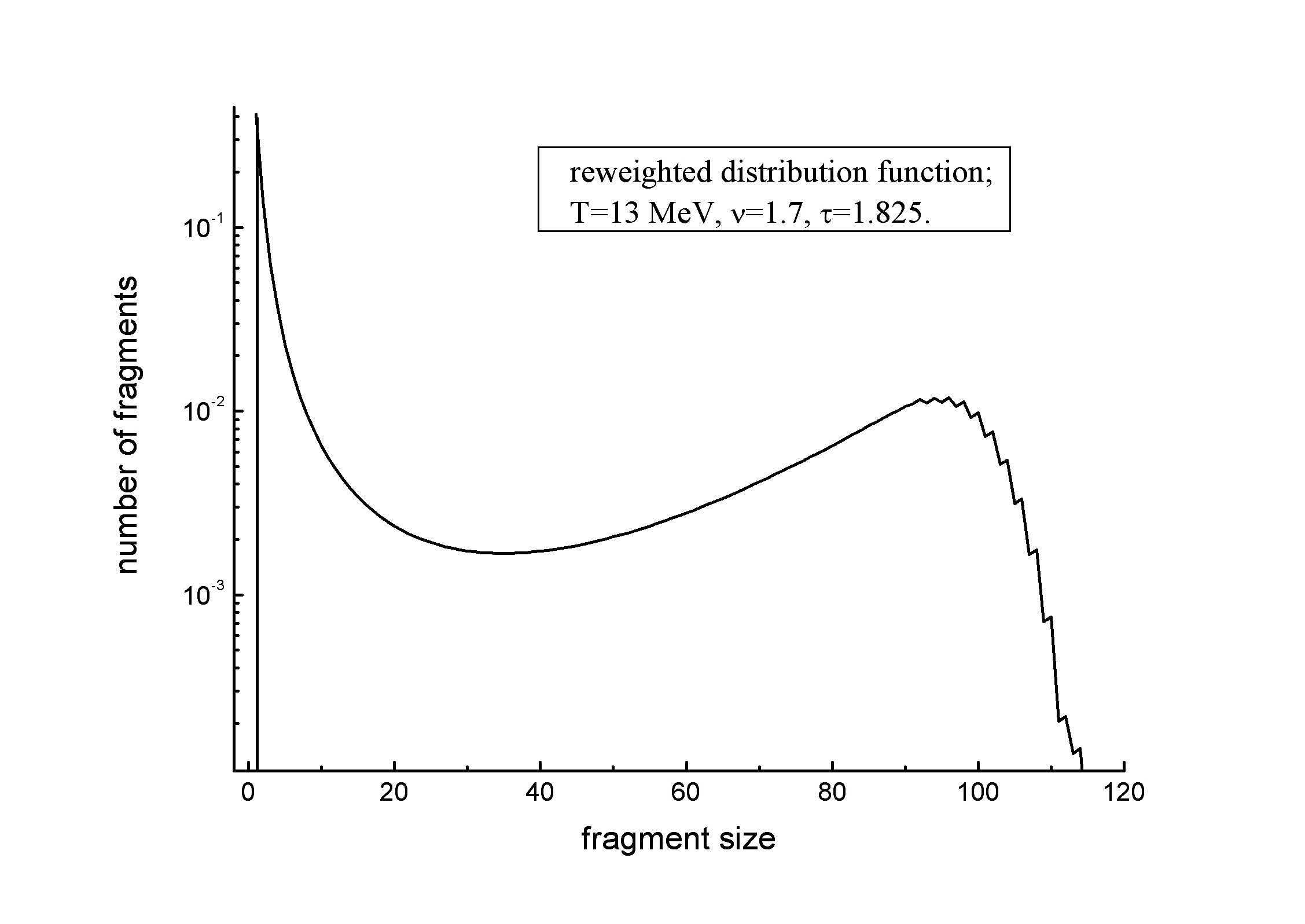
Figure 9: The reweighted fragment size distribution for a finite analog of gaseous phase. The original fragment size distribution corresponds to the parameters $T=13MeV$ and $\nu_{0}=1.7$ MeV (see the corresponding curve in Fig. 8) , but for $K(V)\in[85;115]$ values distributed normally with the mean value $\bar{K}(V)=100$ and a dispersion $5$.

Also the above analysis demonstrates that the finite volume analog of the tricritical point with the parameters $Re(\nu)=0$ and $\sigma(T)=0$, i.e. a state at which the gaseous phase pressure coincides with the pressure of infinite liquid droplet and the surface free energy is zero, belongs to a finite volume analog of a gaseous phase, since according to the above analysis such equalities for finite systems can be achieved only at $T=T_{cep}$ and only for $\nu_{0}=Re(\nu_{0})=0$. Note that at the finite volume analog of the tricritical point the size distribution of the fragments is purely power like. It is hoped that such a feature can be helpful for an experimental identification of the tricritical point in the experiments.

An existence of the gaseous phase with $\nu_{0}>0$ in finite systems clearly indicates the principal difference between the properties of gaseous phases existing in finite and in infinite volumes. And this principal difference can be seen in the fragment distributions shown in Figs. 3 and 8. Indeed, the fragment size distributions depicted in Fig. 3 are monotonically decreasing ones, even taken at the boundary between the macroscopic gaseous phase and macroscopic mixed phase, whereas for $\nu_{0}>0$ the fragment size distributions of Fig. 8 have a bimodal shape. The latter might not look as a canonical bimodal shape, but if one accounts for the fluctuation of the maximal number of nucleons in the system which is similar to the number of participating nucleons in the nuclear reaction, then the resulting distribution may look much more similar to those one discussed in Refs. [3, 4, 5]. In Fig. 9 we show such a reweighted distribution which was constructed from fifteen distributions having the same values of $T=13$ MeV and $\nu_{0}=1.7$ MeV, but for the parameter $K(V)$ distributed normally in the range $K(V)\in[85;115]$ with the mean value $\bar{K}(V)=100$ and a dispersion $5$. Such a reweighting models the possible dynamical fluctuations of the impact parameter in the nuclear reaction. The example of Fig. 9 demonstrates that the observed fragment size distribution does differ from the original statistical fragment size distribution due to weak dynamical fluctuations of the impact parameter. The effect of the dynamical fluctuations of the initial temperature (which appears at the moment of thermal equilibrium) that is well-known in the high energy hadron and nuclear collisions [44] can be even more dramatic and it can essentially modify the original statistical fragment size distribution. The worst is that it is entirely unclear how this cause or/and the other possible physical ones like a collective flow and its instabilities modify the original statistical fragment size distribution before it is measured by a detector. Therefore, from this example and the counterexamples given above we conclude that it is hard to believe that the theoretical schemes suggested in [1, 2, 3, 4] to manipulate with the observed data are, indeed, able to elucidate any essential PT related characteristics of the statistical distributions from the measured data.

4 Conclusions

In the present work we gave two explicit counterexamples to the widely spread beliefs [1, 2, 4, 5, 13] about an exclusive role of bimodality as the first order PT signal and showed that the bimodal distributions can naturally appear both in infinite and in finite systems without a PT. In the first counterexample a bimodal distribution is generated at the supercritical temperatures by the negative values of the surface tension coefficient. This result is in line with the previously discussed role of the competition between the volume and the surface parts of the system free energy [10, 12]. In the second considered counterexample a bimodal fragment distribution is generated by positive values of the effective chemical potential in a finite volume analog of a gaseous phase. The latter was provided by an exact analytical solution of the CSMM for finite systems [15, 12] which was successfully generalized here for more realistic equations of state of the compressible nuclear liquid and for more realistic treatment of the surface tension free energy.

Also here we gave analytic results showing for the first time that for finite, but large systems, the value of the effective chemical potential on the finite volume analog of the $T-\nu$ phase diagram [15, 12] is solely defined by the surface tension coefficient and by the radius of the largest fragment. The derived analytical formulas for partial pressures of the metastable states belonging to the same grand canonical partition give an explicit example that, on the contrary to the beliefs of Refs. [1, 2, 3, 4, 13], in finite systems there are no two ‘pure’ phases as it is the case in the thermodynamic limit. At finite pressures the liquid-like finite droplet appears only as a part of a finite volume analog of a mixed phase. Additionally, here we demonstrated that for positive values of the effective chemical potential $\nu_{0}$ the properties of the gaseous phase in finite systems drastically differ from its properties in the thermodynamic limit. The bimodal fragment size distributions depicted in Figs. 8 and 9 cannot exist in the gaseous phase treated in the thermodynamic limit (see Fig. 3 for comparison).

The above results are in line with the critique [10, 11, 12] of a bimodality as a reliable signal of the PT existence in finite systems. Once more we have to stress that without studying the nature of the bimodal distributions one cannot claim that a PT is its only origin. An interesting result on the bimodality absence in the systems indicating a possible PT existence in multifragment production in heavy-ion nuclear collisions was reported in [45]. This is an additional counterexample to the widely spread belief on an exclusive role of bimodality as a PT signal in finite systems.

Therefore, all the counterexamples obtained in this work on the basis of an exactly solvable statistical model known as the CSMM allow us to conclude that it is rather doubtful that the theoretical schemes invented in Refs. [1, 2, 3, 4] to manipulate with the observed data are, indeed, able to elucidate the reliable PT signals from the measured data.

Acknowledgments. We appreciate the valuable comments of I. N. Mishustin and L. M. Satarov. Also the authors acknowledge a partial support of the Program “Fundamental Properties of Physical Systems under Extreme Conditions” launched by the Section of Physics and Astronomy of the National Academy of Sciences of Ukraine.

References

- [1] Ph. Chomaz, F. Gulminelli and V. Duflot, Phys. Rev. E 64, 046114 (2001).
- [2] Ph. Chomaz and F. Gulminelli, Preprint GANIL-02-19 (2002).
- [3] F. Gulminelli, Ann. Phys. Fr. 29, 6 (2004) and references therein.
- [4] F. Gulminelli, Nucl. Phys. A 791, 165 (2007).
- [5] O. Lopez and M. F. Rivet, Eur. Phys. J. A 30, 263 (2006) and references therein.
- [6] M. Pichon et al. (INDRA and ALADIN Collaborations), Nucl. Phys. A 779, 267 (2006).
- [7] M. Bruno et al., Nucl. Phys. A 807, 48 (2008).
- [8] E. Bonnet et al. (INDRA and ALADIN Collaborations), Phys. Rev. Lett. 103, 072701 (2009).
- [9] C. N. Yang and T. D. Lee, Phys. Rev. 87, 404 (1952).
- [10] L. G. Moretto, J. B. Elliott and L. W. Phair, Mesoscopy and Thermodynamics, proceedings of the conference “World Consensus Initiative III”, Texas A & M University, College Station, Texas, USA, February 11-17, 2005 (see http://cyclotron.tamu.edu/wci3/newer/chapVI_4.pdf).
- [11] O. Lopez, D. Lacroix, and E. Vient, Phys. Rev. Lett. 95, 242701 (2005).
- [12] K. A. Bugaev, Phys. Part. Nucl. 38, 447 (2007).
- [13] T. L. Hill, Thermodynamics of small systems (Dover, New York 1994).
- [14] D. H. E. Gross, Microcanonical Thermodynamics: Phase Transitions in Finite Systems, Lecture Notes in Physics, vol. 66 (World Scientific, 2001).
- [15] K. A. Bugaev, Acta. Phys. Polon. B 36, 3083 (2005).
- [16] J. P. Bondorf et al., Phys. Rep. 257, 131 (1995).
- [17] K. A. Bugaev, M. I. Gorenstein, I. N. Mishustin and W. Greiner, Phys. Rev. C 62, 044320 (2000); arXiv:nucl-th/0007062 (2000); Phys. Lett. B 498, 144 (2001); arXiv:nucl-th/0103075 (2001).
- [18] P. T. Reuter and K. A. Bugaev, Phys. Lett. B 517, 233 (2001).
- [19] K. A. Bugaev, L. Phair and J. B. Elliott, Phys. Rev. E 72, 047106 (2005).
- [20] K. A. Bugaev and J. B. Elliott, Ukr. J. Phys. 52, 301 (2007).
- [21] K. A. Bugaev, arXiv:1012.3400 [nucl-th].
- [22] K. A. Bugaev, A. I. Ivanitskii, E. G. Nikonov, A. S. Sorin and G. M. Zinovjev, Can We Rigorously Define Phases in a Finite System?, Chapter 18 of the Proceedings of the XV-th Research Workshop “Nucleation Theory and Applications”, held at JINR, Dubna, Russia, April 1- 30, 2011, edited by J. W. P. Schmelzer, G. Ropke, V. B. Priezzhev, Dubna JINR, 2011; arXiv:1106.5939 [nucl-th]
- [23] S. Das Gupta and A.Z. Mekjian, Phys. Rev. C 57, 1361 (1998).
- [24] L. Beaulieu et al. (ISiS Collaboration), Phys. Lett. B 463, 159 (1999).
- [25] J. B. Elliott et al., (EOS Collaboration), Phys. Rev. C 62, 064603 (2000).
- [26] L. Van Hove, Physica 15, 951 (1949).
- [27] L. Van Hove, Physica 16, 137 (1950).
- [28] M. I. Gorenstein, D. H. Rischke, H. Stocker, W. Greiner and K. A. Bugaev, J. Phys. G 19, L69 (1993).
- [29] D. Vretenar, T. Niksic, and P. Ring, Phys. Rev. C 68, 024310 (2003).
- [30] G. Colo and Nguyen Van Giai, Nucl. Phys. A 731, 15 (2004).
- [31] V. B. Soubbotin, V. I. Tselyaev and X. Vinas, Phys. Rev. C 69, 064312 (2004).
- [32] E. Khan, Phys. Rev. C 80, 011307(R) (2009).
- [33] see, for instance, H. E. Stanley, Introduction to phase transitions and critical phenomena (Clarendon Press, Oxford, 1971).
- [34] M. E. Fisher, Physics 3, 255 (1967).
- [35] K. A. Bugaev, Phys. Rev. C 76, 014903 (2007); and Phys. Atom. Nucl. 71, 1615 (2008) .
- [36] K. A. Bugaev, V. K. Petrov and G. M. Zinovjev, Phys. Part. Nucl. Lett. 9, 238 (2012); arXiv:0904.4420 [hep-ph] (2009).
- [37] K. A. Bugaev, V. K. Petrov and G. M. Zinovjev, Europhys. Lett. 85, 22002 (2009); Phys. Rev. C 79, 054913 (2009).
- [38] A. I. Ivanytskyi, Nucl. Phys. A 880, 12 (2012).
- [39] K. A. Bugaev and G. M. Zinovjev, Nucl. Phys. A 848, 443 (2010).
- [40] K. A. Bugaev, A. I. Ivanitskii, E. G. Nikonov, V. K. Petrov, A. S. Sorin and G. M. Zinovjev, Phys. Atom. Nucl. 75, 707 (2012).
- [41] J. B. Elliott, K. A. Bugaev, L. G. Moretto and L. Phair, arXiv:0608022 [nucl-ex].
- [42] J. Gross, J. Chem. Phys. 131, 204705 (2009).
- [43] N. Buyukcizmeci et al., arXiv:1211.5990v2 [nucl-th].
- [44] G. Wilk and Z. Wlodarczyk, Eur. Phys. J. A 40, 299 (2009).
- [45] J. D. Frankland et al. [INDRA and ALADIN Collaborations], Phys. Rev. C 71, 034607 (2005).