A Systematically Empirical Evaluation of Vulnerability Discovery Models: a Study on Browsers’ Vulnerabilities

Abstract

A precise vulnerability discovery model (VDM) will provide a useful insight to assess software security, and could be a good prediction instrument for both software vendors and users to understand security trends and plan ahead patching schedule accordingly. Thus far, several models have been proposed and validated. Yet, no systematically independent validation by somebody other than the author exists. Furthermore, there are a number of issues that might bias previous studies in the field. In this work, we fill in the gap by introducing an empirical methodology that systematically evaluates the performance of a VDM in two aspects: quality and predictability. We further apply this methodology to assess existing VDMs. The results show that some models should be rejected outright, while some others might be adequate to capture the discovery process of vulnerabilities. We also consider different usage scenarios of VDMs and find that the simplest linear model is the most appropriate choice in terms of both quality and predictability when browsers are young. Otherwise, logistics-based models are better choices.

1 Introduction

Vulnerability discovery models (VDMs) operate on known vulnerability data to estimate the total number of vulnerabilities that will be reported after the release of a software. Successful models can be useful instruments for both software vendors and users to understand security trends, plan patching schedules, decide updates and forecast security investments in general.

A VDM is a parametric mathematical function counting the number of cumulative vulnerabilities of a software at an arbitrary time $t$. For example, if $\Omega(t)$ is the cumulative number of vulnerabilities at time $t$, the function of the linear model (LN) is $\Omega(t)=At+B$ where $A,B$ are two parameters of LN, which are calculated from the historical vulnerability data.

Fig. 1 sketches a taxonomy of the major VDMs. It includes Anderson’s Thermodynamic (AT) model [5], Rescorla’s Quadratic (RQ) and Rescorla’s Exponential (RE) models [19], Alhazmi & Malaiya’s Logistic (AML) model [1], AML for Multi-version [11], Weibull model (JW) [10], and Folded model (YF) [24]. The goodness-of-fit of these models, i.e. how well a model could fit the numbers of discovered vulnerabilities, is normally evaluated in each paper on a specific vulnerability data set, except AML which has been validated for different types of application (i.e. operating system [4, 3], browsers [22], web servers [2, 23]). Yet, no independent validation by somebody other than the authors exists. Furthermore, a number of issues might bias the results of previous studies.

• Firstly, many studies did not clearly define what a vulnerability is. Indeed different definitions of vulnerability might lead to different counted numbers of vulnerabilities, and consequently, different conclusions.

• Secondly, all versions of a software were considered as a single “entity”. Even though there is a large amount of shared code, they are still different by a non-negligible amount of code.

• Thirdly, the goodness-of-fit of the models was often evaluated at a single time point (of writing their papers) and not used as a predictor e.g., to forecast data for the next quarter for instance.

A detail discussion about these issues is available later in section §3.

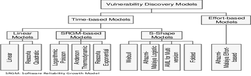
Fig. 1: Taxonomy of Vulnerability Discovery Models.

In this paper we want to address these shortcomings and derive a methodology that can answer two basic questions concerning VDM: “Are VDMs adequate to capture the discovery process of vulnerabilities?”, and “which VDM is the best?”.

1.1 Contributions of This Paper

The contributions of this work are detailed below:

• We proposed an experimental methodology to assess the performance of a VDM based on its goodness-of-fit quality and predictability.

• We demonstrated the methodology by conducting an experiment analyzing eight VDMs, including AML, AT, JW, RQ, RE, LP, LN, and YF on 30 major releases of four popular browsers Internet Explorer (IE), Firefox (FF), Chrome and Safari.

• We presented an empirical evidence for the adequacy of the VDMs in terms of quality and predictability. The AT and RQ models are not adequate; whereas all other models may be adequate when software is young (12 months). However only s-shape models (AML, JW, YF) should be considered when software is middle age (36 months) or older.

• We compared these VDMs (except AT and RQ) in different usage scenarios in terms of predictability and quality. The simplest model, LN, is more appropriate than other complex models when software is young and the prediction time span is not too long (12 months or less). Otherwise, the AML model is superior. These results are summarized in Table I.

The rest of the paper is organized as follows. Section §2 presents terminology in our work. The research questions are presented in section §3 and the proposed methodology is described in section §4. Next, we apply the methodology to analyze the empirical performance of VDMs in all data sets in section §5. Then in section §6, we discuss the threats to the validity of our work. Finally, we review related work in section §7, and conclude in section §8.

Table I: Performance summary of VDMs.

Model	Performance
AT, RQ	should be rejected due to low quality.
LN	is the best model for first 12 months(∗).
AML	is the best model for $13^{th}$ to $36^{th}$ month (∗).
RE, LP	may be adequate for first 12 months (∗∗).
JW, YF	may be adequate for $13^{th}$ to $36^{th}$ month(∗).

^(∗): in terms of quality and predictability for next 3/6/12 months.
^(∗∗): in terms of quality and predictability for next 3 months.

2 Terminology

• A vulnerability is “an instance of a [human] mistake in the specification, development, or configuration of software such that its execution can [implicitly or explicitly] violate the security policy”[12], later revised by [18]. The definition covers all aspects of vulnerabilities discussed in [6, 7, 8, 20], see also [18] for a discussion.

• A data set is a collection of vulnerability data extracted from one or more data sources.

• A release refers to a particular version of an application e.g., Firefox v1.0.

• A horizon is a specific time interval sample. It is measured by the number of months since the released date, e.g., from month $1$ to $12$ months after the release.

• An observed vulnerability sample (or observed sample, for short) is a time series of monthly cumulative vulnerabilities of a major release since the first month after release to a particular horizon.

• An evaluated sample is a tuple of an observed sample, a VDM model fitted to this sample (or another observed sample), and the goodness-of-fit of this model to this sample.

3 Research Questions and Methodology Overview

In this work, we address the following two questions:

RQ1

How to evaluate the performance of a VDM?

RQ2

How to compare between two or more VDMs?

We propose a methodology to answer these questions. The proposed methodology identifies data collection steps and mathematical analyses to empirically assess different performance aspects of a VDM . The methodology is summarized in Table II.

Table II: Methodology overview.

Step 1 Acquire the vulnerability data
desc.	Identify the vulnerability data sources, and the way to count vulnerabilities. If possible, different vulnerability sources should be used to select the most robust one. Observed samples then can be extracted from collected vulnerability data.
input	Vulnerability data sources.
output	Set of observed samples.
criteria	CR1 Collection of observed samples • Vulnerabilities should be counted for individual releases (possibly by different sources). • Each observable sample should have at least $5$ data points.
Step 2 Fit the VDM to observed samples
desc.	Estimate the parameters of the VDM formula to fit observed samples as much as possible. The $\chi^{2}$ goodness-of-fit test is employed to assess the goodness-of-fit of the fitted model based on criteria II.
input	Set of observed samples.
output	Set of evaluated samples.
criteria	CR2 The classification of the evaluated samples based on the p-value of a $\chi^{2}$ test. • Good Fit: $\textit{p-value}\in[0.80,1.0]$, a good evidence to accept the model. We have more than $80\%$ chances of generating the observed sample from the fitted model. • Not Fit: $\textit{p-value}\in[0,0.05)$, a strong evidence to reject the model. It means less than $5\%$ chances that the fitted model would generate the observed sample. • Inconclusive Fit: $\textit{p-value}\in[0.05,0.80)$, there is not enough evidence to neither reject nor accept the fitted model.
Step 3 Perform goodness-of-fit quality analysis
desc.	Analyze the goodness-of-fit quality of the fitted model by using the temporal quality metric which is the weighted ratio between fitted evaluated samples (both Good Fit and Inconclusive Fit) and total evaluated samples.
input	Set of evaluated samples.
output	Temporal quality metric.
criteria	CR3 The rejection of a VDM. A VDM is rejected if it has a temporal quality lower than 0.5 even by counting Inconclusive Fits samples as positive (with weight 0.5). Different periods of software lifetime could be considered: • $12$ months (young software) • $36$ months (middle-age software) • $72$ months (old software)
Step 4 Perform predictability analysis
desc.	Analyze the predictability of the fitted model by using the predictability metric. Depending on different usage scenarios, we have different observation periods and time spans that the fitted model supposes to be able to predict. This is described in II.
input	Set of evaluated samples.
output	Predictability metric.
criteria	CR4 The observation period and prediction time spans based on some possible usage scenarios. Observation Prediction Scenario Period (months) Time Span (months) Plan for short-term support 6–24 3 Plan for long-term support 6–24 12 Upgrade or keep 6–12 6 Historic analysis 24–36 12
Step 5 Compare VDM
desc.	Compare the quality of the VDM with other VDMs by comparing their temporal quality and predictability metrics.
input	Temporal quality and predictability measurements of models in comparison.
output	Ranks of models.
criteria	CR5 The comparison between two VDM A VDM $\textit{vdm}_{1}$ is better than a VDM $\textit{vdm}_{2}$ if: • either the predictability of $\textit{vdm}_{1}$ is significantly greater than that of $\textit{vdm}_{2}$, • or there is no significant difference between the predictability of $\textit{vdm}_{1}$ and $\textit{vdm}_{2}$, but the temporal quality of $\textit{vdm}_{1}$ is significantly greater than that of $\textit{vdm}_{2}$. The temporal quality and predictability should have their horizons and prediction time spans in accordance to criteria II and II. Furthermore, a controlling procedure for multiple comparisons should be considered.

In order to satisfactorily answer the questions above, we must address some biases that potentially affected the validity of previous studies.

The vulnerability definition bias may affect the vulnerability data collection process. Indeed all previous studies reported their data sources, but none clearly mentioned what a vulnerability is, and how to count it. A vulnerability could be either an advisory reported by a software vendor such as Mozilla Foundation Security Advisory – MFSA, or a security bug causing software to be exploited (reported in Mozilla Bugzilla), or an entry in third-party vulnerability databases (e.g., National Vulnerability Database – NVD). Some entries may be classified differently by different entities: a third-party database might report vulnerabilities, but the security bulletin of vendors may not classify them as such. Consequently, the counted number of vulnerabilities could be widely different depending on the different definitions.

Example 1   Fig. 2 exemplifies this issue. A security flaw concerning the buffer overflow and use-after-free of Firefox v13.0 is reported in three databases with different number of entries: one MFSA entry (mfsa-2012-40), three Bugzilla entries (744541, 747688, and 750066), and three NVD entries (cve-2012-1947, cve-2012-1940, and cve-2012-1941). The cross references among these entries are illustrated as directional connections. This figure raises a question “how many vulnerabilities should we count in this case?”.  

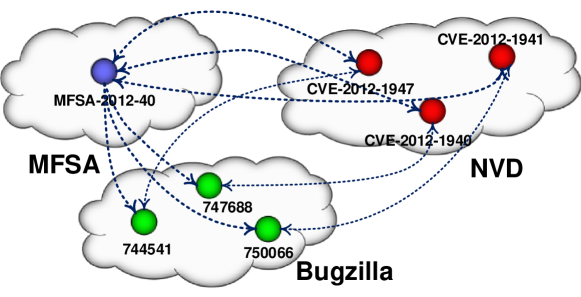
A buffer-overflow flaw is reported in one entry of MFSA, three entries of Bugzilla, and three entries of NVD. There are cross-references among entries (arrow-headed dotted lines). So, how many vulnerabilities should we count?

Fig. 2: The problem of counting vulnerabilities in Firefox.

The multi-version software bias affects the count of vulnerability across releases. Some studies (e.g., [22, 23]) considered all versions of software as a single entity, and counted vulnerabilities for this entity. Our previous study [13] has shown that each Firefox version has its own code base, which may differ by $30\%$ or more from the immediately preceding one. Therefore, as time goes by, we can no longer claim that we are counting the vulnerabilities of the same application.

Example 2   Fig. 3 visualizes this problem in a plot of the cumulative vulnerabilities of Firefox v1.0, Firefox v1.5, and Firefox v1.0-1.5 as a single entity. Clearly, the function of the “global” version should be different from the functions of the individual versions.  

The overfitting bias, as name suggested, concerns the ability of a VDM to explain history in hindsight. Previous studies took a snapshot of vulnerability data, and fitted this entire snapshot to a VDM. This made a brittle claim of fitness: the claim was only valid at the time vulnerabilities were collected. It explained history but did not tell us anything about the future. Meanwhile, we are interested in the ability of a VDM to be a good “law of nature” that is valid across releases and time and to some predict extent the future.

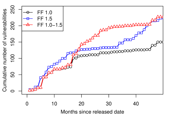
This shows the cumulative vulnerabilities of Firefox v1.0, v1.5, and v1.0-v1.5 as a single entity. The “global” entity exhibits a trend that is not present in the “individual” versions.

Fig. 3: Global vs individual vulnerability trends for Firefox.

4 Methodology Details

This section discusses the details of our methodology to evaluate the performance of a VDM.

4.1 II: Acquire the Vulnerability Data

The acquisition of vulnerability data consists of two sub steps: Data set collection, and Data sample extraction.

During Data set collection, we identify the data sources to be used for the study (as they may not equally fit to the task). We can classify them as follows:

• Third-party advisory ($\sf TADV$): is a vulnerability database maintained by a third-party organization (not software vendors) e.g., $\sf NVD$, Open Source Vulnerability Database ($\sf OSVDB$).

• Vendor advisory ($\sf ADV$): is a vulnerability database maintained by a software vendor, e.g., MFSA, Microsoft Security Bulletin. Vulnerability information in this database could be announced from third-party, but it is always validated before being announced as an advisory.

• Vendor bug tracker ($\sf BUG$): is a bug-tracking database, usually maintained by vendors.

For our purposes, the following features of a vulnerability are interesting and must be provided:

• Identifier ($\sf id$): is the identifier of a vulnerability within a data source.

• Disclosure date ($\sf date$): refers to the date when a vulnerability is reported to the database.

• Vulnerable Releases ($\sf R$): is a list of releases affected by a vulnerability.

• References ($\sf refs$): is a list of reference links to other data sources.

Not every feature is available from all data sources. To obtain missing features, we can use $\sf id$ and $\sf refs$ to link across data sources and extract the expected features from secondary data sources.

Example 3   Vulnerabilities of Firefox are reported in three data sources: NVD, MFSA, and Mozilla Bugzilla. Neither MFSA nor Bugzilla provides the Vulnerable Releases feature, but NVD does. Each MFSA entry has one or more links to NVD and Bugzilla. Therefore, we could to combine MFSA and NVD, Bugzilla and NVD to obtain the missing data.  

We address the vulnerability definition bias by taking into account different definitions of vulnerability. Particularly, we collected different vulnerability data sets with respect to these definitions. We also address the multi-version issue by collecting vulnerability data for individual releases. Table III shows different data sets that we have considered in our study. They are combinations of three types of data sources : third-party (i.e. NVD as a representative), vendor advisory, and vendor bug tracker. The English descriptions of these data sets for a release $r$ are as follows:

• $\sf NVD(\emph{r})$: a set of NVD entries which claim $r$ is vulnerable.

• $\sf NVD.Bug(\emph{r})$: a set of NVD entries which are confirmed by at least a vendor bug report, and claim $r$ is vulnerable.

• $\sf NVD.Advice(\emph{r})$: a set of NVD entries which are confirmed by at least a vendor advisory, and claim $r$ is vulnerable. Notice that the advisory report might not mention $r$, but later releases.

• $\sf NVD.Nbug(\emph{r})$: a set of vendor bug reports confirmed by NVD, and $r$ is claimed vulnerable by NVD.

• $\sf Advice.NBug(\emph{r})$: a set of bug reports mentioned in an advisory report of a vendor. The advisory report also refers to at least an $\sf NVD$ entry that claims $r$ is vulnerable.

Table III: Formal definition of data sets.

Data set	Definition
NVD($r$)	$\left\{{\sf nvd\in{\sf NVD}|r\in R_{nvd}}\right\}$
NVD.Bug($r$)	$\left\{{\sf nvd\in{\sf NVD}|\exists b\in BUG:r\in R_{nvd}\wedge id_{\sf b}\in refs_{\sf nvd}}\right\}$
NVD.Advice($r$)	$\left\{{\sf nvd\in{\sf NVD}|\exists a\in ADV:r\in R_{nvd}\wedge id_{\sf a}\in refs_{\sf nvd}}\right\}$
NVD.NBug($r$)	$\left\{{\sf b\in BUG|\exists nvd\in NVD:r\in R_{nvd}\wedge id_{\sf b}\in refs_{\sf nvd}}\right\}$
Advice.NBug($r$)	$\left\{{\sf b\in BUG|\exists a\in ADV,\exists nvd\in NVD:r\in R_{nvd}}\right.$
	$\left.{\sf\wedge id_{b}\in refs_{a}\wedge id_{nvd}\in refs_{a}\wedge\operatorname{cluster}_{a}(id_{b},id_{nvd})}\right\}$

Note: ${\sf R_{nvd},refs_{\sf nvd}}$ denote the vulnerable releases and references of an entry $\sf nvd$, respectively. ${\sf id_{\sf a},id_{\sf b},id_{nvd}}$ denote the identifier of $\sf a$, $\sf b$, and $\sf nvd$. $\operatorname{cluster}_{\sf a}({\sf id_{b},id_{nvd}})$ is a predicate checking whether ${\sf id_{b}}$ and ${\sf id_{nvd}}$ are located next together in the advisory ${\sf a}$.

For Data sample extraction, we extract observed samples from collected data sets. An observed sample is a time series of (monthly) cumulative vulnerabilities of a release. It starts from the first month since release to the end month, called horizon. A month is an appropriate granularity for sampling because week and day are too short intervals and are subject to random fluctuation. Additionally, this granularity was used in the literature.

Let $R$ be the set of analyzed releases and $DS$ be the set of data sets, an observed sample (denoted as os) is a time series defined as follows:

$$\textit{os}={\footnotesize\textsf{TS}}(r,ds,{\tau})$$ (1)

where:

• $r\in R$ is a release in the evaluation;

• $ds\in DS$ is the data set where samples are extracted;

• ${\tau}\in{\mathrm{T}}_{r}=\left[{\tau}^{r}_{min},{\tau}^{r}_{max}\right]$ is the horizon of the observed sample, in which ${\mathrm{T}}_{r}$ is the horizon range of release $r$.

In the horizon range of release $r$, the minimum value of horizon ${\tau}^{r}_{min}$ of $r$ depends on the starting time of the first observed sample of $r$. Here we choose ${\tau}^{r}_{min}=6$ for all releases so that all observed samples have enough data points for fitting all VDMs. The maximum value of horizon ${\tau}^{r}_{max}$ depends on how long the data collection period is for each release.

Example 4   IE v4.0 was released in September, $1997$. The first month was on $31$ October, $1997$. The first observed sample of IE v4.0 is a time series of $6$ numbers of cumulative vulnerabilities for the $1^{st},2^{nd},\ldots,6^{th}$ months. Since the date of data collection is on 01 July 2012, IE v4.0 have been released for 182 months, and therefore has 177 observed samples. Hence the maximum value of horizon (${\tau}^{\sf IEv4.0}_{max}$) is $182$.  

4.2 II: Fit a VDM to Observed Samples

We estimate the parameters of the VDM formula by a regression method so that the VDM curve fits an observed sample as much as possible. We denote the fitted curve (or fitted model) as:

$$\textit{vdm}_{{\footnotesize\textsf{TS}}(r,ds,{\tau})}$$ (2)

where $vdm$ is the VDM being fitted; $\textit{os}={\footnotesize\textsf{TS}}(r,ds,{\tau})$ is an observed sample from which the vdm’s parameters are estimated. (2) could be shortly written as $\textit{vdm}_{\textit{os}}$.

Example 5   Fitting the AML model to the NVD data set of Firefox v3.0 at the $30^{th}$ month, i.e. the observed sample $\textit{os}={\footnotesize\textsf{TS}}({\sf FF3.0},{\sf NVD},30)$, generates the curve:

$$\textit{AML}_{{\footnotesize\textsf{TS}}({\sf FF3.0},{\sf NVD},30)}=\frac{183}{183\cdot 0.078\cdot e^{-0.001\cdot 183\cdot t}+1}$$

Fig. 4 illustrates the plots of three curves $\textit{AML}_{{\footnotesize\textsf{TS}}(r,{\sf NVD},30)}$, where $r$ is $\sf FF3.0,FF2.0$, and $\sf FF1.0$. The X-axis is the number of months since release, and the Y-axis is the cumulative number of vulnerabilities. Circles represent observed vulnerabilities. The solid line indicates the fitted AML curve.  

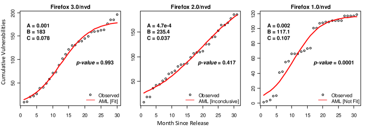
A,B,C are three parameters in the formula of the AML model: $\Omega(t)=\frac{B}{BCe^{-ABt}+1}$ (see also Table IV)

Fig. 4: Fitting the AML model to the $\sf NVD$ data sets for Firefox v3.0, v2.0, and v1.0.

In Fig. 4, the distances of the circles to the curve are used to estimate the goodness-of-fit of the model. The goodness-of-fit is measured by the Pearson’s Chi-Square ($\chi^{2}$) test, which is a common test in the literature. In this test, we measure the $\chi^{2}$ statistic value of the curve by using the following formula:

$$\chi^{2}=\sum_{t=1}^{{\tau}}\frac{(O_{t}-E_{t})^{2}}{E_{t}}$$ (3)

where $O_{t}$ is the observed cumulative number of vulnerabilities at time $t$ (i.e. $t^{\textnormal{th}}$ value of the observed sample); $E_{t}$ denotes the expected cumulative number of vulnerabilities which is the value of the curve at time $t$. The $\chi^{2}$ value is proportional to the differences between the observed values and the expected values. Hence, the larger $\chi^{2}$, the smaller goodness-of-fit. If the $\chi^{2}$ value is large enough, we can safely reject the model. In other words, the model statistically does not fit the observed data set. The $\chi^{2}$ test requires all expected values should be at least $5$ to ensure the validity of the test [17, Chap. 1]. If there is any expected value is less than 5, we need to combine some first months to increase the expected value i.e. increase the starting value of $t$ in (3) until $E_{t}\geq 5$.

The conclusion about whether a VDM curve statistically fits an observed sample relies on the p-value of the test, which is derived from $\chi^{2}$ value and the degrees of freedom (i.e. the number of months minus one). Semantically, the p-value is the probability that we falsely reject the null hypothesis when it is true (i.e. error Type I: false positive). The null hypothesis here is: “there is no statistical difference between observed and expected values.” which means that the model fits the observed sample. Therefore, if the p-value is less than the significance level $\alpha$ of $0.05$, we can reject a VDM because there is less than $5\%$ chances that this fitted model would generate the observed sample.

In contrast, to accept a VDM, we exploit the power of the $\chi^{2}$ test which is the probability of rejecting the null hypothesis when it is false. Normally, ‘an $80\%$ power is considered desirable’ [15, Chap. 8]. Hence we accept a VDM if the p-value is greater than or equal to $0.80$. We have more than $80\%$ chances of generating the observed sample from the fitted curve. In all other cases, we should neither accept nor reject the model (inconclusive fit).

The criteria II in Table II summarizes the way by which we assess the goodness-of-fit of a fitted model based on the p-value of the $\chi^{2}$ test.

In the sequel, we use the term evaluated sample to denote the triplet composed by an observed sample, a fitted model, and the p-value of the $\chi^{2}$ test.

Example 6   In Fig. 4, the first plot shows the AML model with a Good Fit ($\textit{p-value}=0.993>0.80$), the second plot exhibits the AML model with an Inconclusive Fit ($0.05<\textit{p-value}=0.417<0.80$), and the last one denotes the AML model with a Not Fit ($\textit{p-value}=0.0001<0.05$).  

There are also other statistic tests for goodness-of-fit, for instance the Kolmogorov-Smirnov (K-S) test, and the Anderson-Darling (A-D) test. The K-S test is an exact test; it, however, only applies to continuous distributions. An important assumption is that the parameters of the distribution cannot be estimated from the data. Hence, we cannot apply it to perform the goodness-of-fit test for a VDM. The A-D test is a modification of the K-S test that works for some distributions [17, Chap. 1] (i.e. normal, log-normal, exponential, Weibull, extreme value type I, and logistic distribution), but some VDMs violate this assumption.

4.3 II: Perform Goodness-of-Fit Quality Analysis

To address the overfitting bias, we introduce the goodness-of-fit quality (or quality, for short) that measures the overall number of Good Fits and Inconclusive Fits among different samples. In contrast, previous studies considered only one observed sample which is the one with the largest horizon in their experiment.

Let $\textit{OS}=\left\{{\footnotesize\textsf{TS}}(r,ds,{\tau})|r\in R\wedge ds\in DS\wedge{\tau}\in{\mathrm{T}}_{r}\right\}$ be the set of observed samples, the overall quality of a model vdm is defined as the weighted ratio of the number of Good Fit and Inconclusive Fit evaluated samples over the total ones, as shown bellow:

$$Q_{\omega}=\frac{|\textit{GES}|+\omega\cdot|\textit{IES}|}{|\textit{ES}|}$$ (4)

where:

• $\textit{ES}=\left\{\left\langle\textit{os},\textit{vdm}_{\textit{os}},p\right\rangle|\textit{os}\in\textit{OS}\right\}$ is the set of evaluated samples generated by fitting vdm to observed samples;

• $\textit{GES}=\left\{\left\langle\textit{os},\textit{vdm}_{\textit{os}},p\right\rangle\in\textit{ES}|p\geq 0.80\right\}$ is the set of Good Fit evaluated samples;

• $\textit{IES}=\left\{\left\langle\textit{os},\textit{vdm}_{\textit{os}},p\right\rangle\in\textit{ES}|0.05\leq p<0.80\right\}$ is the set of Inconclusive Fit evaluated samples;

• $\omega\in[0..1]$ is the inconclusiveness contribution factor denoting that an Inconclusive Fit is $\omega$ times less important than a Good Fit.

Example 7   If we fit the AML model to $3,895$ observed samples of the four browsers IE, Firefox, Chrome, and Safari. For $1,526$ times AML is a Good Fit, and for $1,463$ times AML is an Inconclusive Fit. The overall quality of AML is:

$$Q_{\omega=0} =\frac{1,526}{3,895}=0.39$$

$$Q_{\omega=1} =\frac{1,526+1,463}{3,895}=0.77$$

$$Q_{\omega=0.5} =\frac{1,526+0.5\cdot 1,463}{3,895}=0.58$$

To calculate the $\chi^{2}$ test we refit the model each and every time. So this means that we have $1,526$ different parameters A, B and C for each good fit curve (see Fig. 4).  

The overall quality metric ranges between 0 and 1. The quality of 0 indicates a completely inappropriate model, whereas the quality of 1 indicates a perfect one. This metric is a very optimistic measure as we are essentially “refitting” the model as more data become available. Hence, it is the upper bound value of the VDM quality.

The factor $\omega$ denotes the contribution of an inconclusive fit to the overall quality. A skeptical analyst would expect $\omega=0$, which means only Good Fits are meaningful. Meanwhile an optimistic analyst would set $\omega=1$, which mean an Inconclusive Fit is as good as a Good Fit. The optimistic choice $\omega=1$ is usually adopted by the proposers of each model in previous studies in the field while assessing the VDM quality. The effect of the $\omega$ factor on the overall quality metrics is illustrated in Fig. 5 showing the variation of the overall quality of two models AML and AT with respect to $\omega$. We do not know whether an Inconclusive Fit is good or not because the observed samples do not provide enough evidence. Hence, the choice of $\omega=0.5$ may be considered a good balance. During our analysis we use $\omega=0.5$; any exception will be explicitly noted.

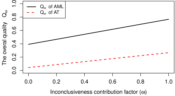
Fig. 5: The variation of the overall quality $Q_{\omega}$ with respect to the $\omega$ factor.

The overall quality metric is sensitive to brittle performance in time. A VDM could produce a lot of Good Fits evaluated samples for the first $6$ months, but almost Not Fits at other horizons. Unfortunately, the metric did not address this phenomenon.

To avoid this unwanted effect, we introduce the temporal quality metric which represents the evolution of the overall quality over time. The temporal quality $Q_{\omega}({\tau})$ is the weighted ratio of the Good Fit and Inconclusive Fit evaluated samples over total ones at the particular horizon $\tau$. The temporal quality is formulated in the following equation:

$$Q_{\omega}({\tau})=\frac{|\textit{GES}({\tau})|+\omega\cdot|\textit{IES}({\tau})|}{|\textit{ES}({\tau})|}$$ (5)

where:

• ${\tau}\in{\mathrm{T}}$ is the horizon that we observe samples, in which ${\mathrm{T}}\subseteq\bigcup_{r\in R}{\mathrm{T}}_{r}$ is the subset of the union of the horizon ranges of all releases $r$ in evaluation;

• $\textit{ES}({\tau})=\left\{\left\langle\textit{os},\textit{vdm}_{\textit{os}},p\right\rangle|\textit{os}\in\textit{OS}({\tau})\right\}$ is the set of evaluated samples at the horizon ${\tau}$; where OS($\tau$) is the set of observed samples at the horizon $\tau$ of all releases;

• $\textit{GES}({\tau})\subseteq\textit{ES}({\tau})$ is the set of Good Fit evaluated samples at the horizon $\tau$;

• $\textit{IES}({\tau})\subseteq\textit{ES}({\tau})$ is the set of Inconclusive Fit evaluated samples at the horizon $\tau$;

• $\omega$ is the same as for the overall quality $Q_{\omega}$.

To study the trend of the temporal quality $Q_{\omega}({\tau})$, we employ the moving average technique which is commonly used in time series analysis to smooth out short-term fluctuations and highlight longer-term trends. Intuitively each point in the moving average is the average of some adjacent points in the original series. The moving average of the temporal quality is defined as follows:

$$\textit{MA}_{k}^{Q_{\omega}}({\tau})=\frac{1}{k}\sum_{i=1}^{k}Q_{\omega}({\tau}-i+1)$$ (6)

where $k$ is the window size. The choice of $k$ changes the spike-smoothening effect: higher $k$, smoother spikes. Additionally, $k$ should be an odd number so that variations in the mean are aligned with variations in the data rather than being shifted in time.

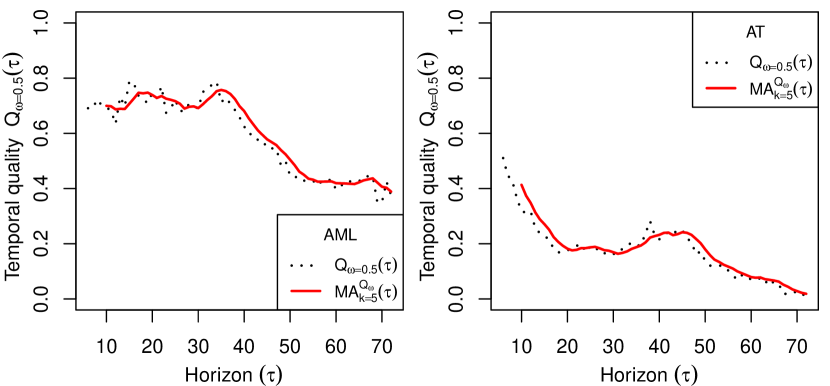
Dotted lines are the temporal quality with $\omega=0.5$, solid lines are the moving average of the temporal quality with the window size $k=5$.

Fig. 6: An example about the moving average of the temporal quality of AML and AT models.

Example 8   Fig. 6 depicts the moving average for the temporal quality of AML and AT models. In this example, we choose a window size $k=5$ because the minimum horizon is six (${\tau}^{r}_{min}=6$), so $k$ should be less than this horizon ($k<{\tau}^{r}_{min}$); and $k=3$ is too small to smooth out the spikes.  

4.4 II: Perform Predictability Analysis

The predictability of a VDM measures the capability of predicting future trends of vulnerabilities. This essentially makes a VDM applicable in practice. The calculation of the predictability of a VDM has two phases, the learning phase and the prediction phase. In the learning phase, we fit a VDM to an observed sample at a certain horizon. In the prediction phase, we evaluate the qualities of the fitted model on observed samples in future horizons.

We extend (5) to calculate the prediction quality. Let $\textit{vdm}_{{\footnotesize\textsf{TS}}(r,ds,{\tau})}$ be a fitted model at horizon $\tau$. The prediction quality of this model in the next $\delta$ months is calculated as follows:

$$Q^{*}_{\omega}({\tau},\delta)=\frac{|\textit{GES}^{*}({\tau},\delta)|+\omega\cdot|\textit{IES}^{*}({\tau},\delta)|}{|\textit{ES}^{*}({\tau},\delta)|}$$ (7)

where:

• $\textit{ES}^{*}({\tau},\delta)=\left\{\left\langle{\footnotesize\textsf{TS}}(r,ds,{\tau}+\delta),\textit{vdm}_{{\footnotesize\textsf{TS}}(r,ds,{\tau})},p\right\rangle\right\}$ is the set of evaluated samples at the horizon ${\tau}+\delta$ in which we evaluate the quality of the model fitted at horizon $\tau$ ($\textit{vdm}_{{\footnotesize\textsf{TS}}(r,ds,{\tau})}$) on observed samples at the future horizon ${\tau}+\delta$. We refer to $\textit{ES}^{*}({\tau},\delta)$ as set of evaluated samples of prediction;

• $\textit{GES}^{*}({\tau},\delta)\subseteq\textit{ES}^{*}({\tau},\delta)$ is the set of Good Fit evaluated samples of prediction at the horizon ${\tau}+\delta$;

• $\textit{IES}^{*}({\tau},\delta)\subseteq\textit{ES}^{*}({\tau},\delta)$ is the set of Inconclusive Fit evaluated samples of prediction at the horizon ${\tau}+\delta$.

• $\omega$ is the same as for the overall quality $Q_{\omega}$.

Example 9   Fig. 7 illustrates the prediction qualities of two models AML and AT starting from the horizon of $12^{th}$ month (${\tau}=12$, left) and $24^{th}$ month (${\tau}=24$, right), and predicting the value for next $12$ months ($\delta=0\ldots 12$). White circles are prediction qualities of AML, and red (gray) circles are those of AT.  

As we can see from Fig. 7 the ability of a model to predict data decreases with time. It is therefore useful to identify some interesting prediction time spans (such as next $6$ months) that can be used for pairwise comparison between VDMs. To this extent, we identify some different scenarios by which we specify the duration of data observation and the prediction time span. Other scenarios may be identified depending on the application or the readers’ interest:

• Plan for short-term support: the data observation period may vary from $6$ months to the whole lifetime. We are looking for the ability to predict the trend in next quarter (i.e. $3$ months) to plan the short-term support activities e.g., allocating resources for fixing vulnerabilities.

• Plan for long-term support: we would like to predict a realistic expectation for bug reports in the next 1 year to plan the long-term activities.

• Upgrade or keep: the data observation period is short (at from 6 to 12 months). We are looking on what is going to happen in next 6 months. For example to decide whether to keep the current system or to go over the hassle of updating it.

• Historic analysis: the data observation period is long (2 to 3 years), we are considering what happens for extra support in the next 1 year.

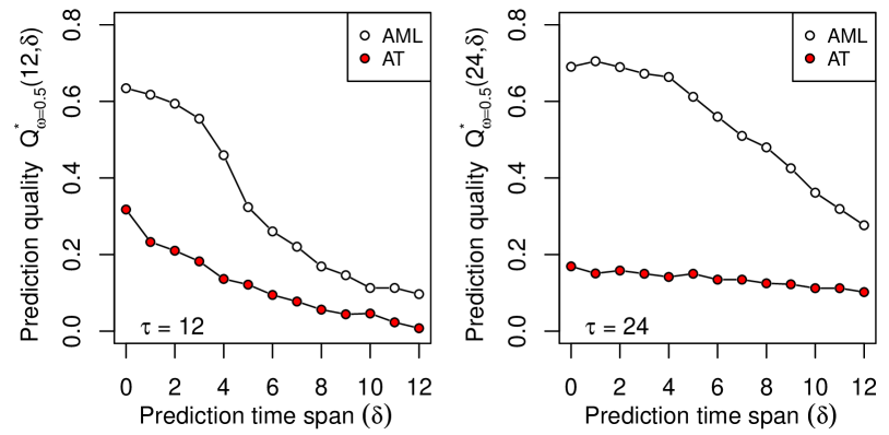
Fig. 7: The prediction qualities of the AML and AT model at some horizons.

We should assess the predictability of a VDM not only along the prediction time span, but also along the horizon to ensure that the VDM is able to consistently predict the vulnerability data in an expected period. To facilitate such assessment we introduce the predictability metric which is the average of prediction qualities at a certain horizon.

The predictability of the curve $\textit{vdm}_{\textit{os}}$ at the horizon $\tau$ in a time span of $\Delta$ months is defined as the average of the prediction quality of $\textit{vdm}_{\textit{os}}$ at the horizon $\tau$ and its $\Delta$ consecutive horizons ${\tau}+1,{\tau}+2,...,{\tau}+\Delta$, as the following equation shows:

$$\textit{Predict}_{\omega}({\tau},\Delta) =\sqrt[\Delta+1]{\prod_{\delta=0}^{\Delta}Q^{*}_{\omega}({\tau},\delta)}$$ (8)

where $\Delta$ is the prediction time span.

In (8), we use the geometric mean instead of the arithmetic mean. The temporal quality is a normalized measure so using the arithmetic mean to average such values might produce a meaningless result, whereas the geometric mean behaves correctly [9].

4.5 II: Compare VDM

This section addresses the second research question 3. The comparison is based on the quality and the predictability of VDMs. The base line for the comparison is that: the better model is a better one in forecasting changes. Hereafter, we discuss how to compare VDM:

Given two models $\textit{vdm}_{1}$ and $\textit{vdm}_{2}$, the comparison between $\textit{vdm}_{1}$ and $\textit{vdm}_{2}$ could be done as below:

We compare the predictability of $\textit{vdm}_{1}$ and that of $\textit{vdm}_{2}$. Let $\rho_{1},\rho_{2}$ be the predictability of $\textit{vdm}_{1}$ and $\textit{vdm}_{2}$, respectively.

$$\rho_{1} =\left\{\textit{Predict}_{\omega=0.5}({\tau},\Delta)|{\tau}=6..{\tau}_{max},\textit{vdm}_{1}\right\}$$ (9)

$$\rho_{2} =\left\{\textit{Predict}_{\omega=0.5}({\tau},\Delta)|{\tau}=6..{\tau}_{max},\textit{vdm}_{2}\right\}$$

where the prediction time span $\Delta$ could follow the criteria II; ${\tau}_{max}=\min(72,\max_{r\in R}{\tau}^{r}_{max})$. We employ the one-sided Wilcoxon rank-sum test to compare $\rho_{1},\rho_{2}$. If the returned p-value is less than the significance level $\alpha=0.05$, the predictability of $\textit{vdm}_{1}$ is stochastically greater than that of $\textit{vdm}_{2}$. It also means that $\textit{vdm}_{1}$ is better than $\textit{vdm}_{2}$. If $\textit{p-value}\geq 1-\alpha$, we conclude the opposite i.e. $\textit{vdm}_{2}$ is better than $\textit{vdm}_{1}$. Otherwise we have not enough evidence either way.

If the previous comparison is inconclusive, we retry the comparison using the value of temporal quality of the VDMs instead of the predictability. We just replace $Q_{\omega=0.5}({\tau})$ for $\textit{Predict}_{\omega=0.5}$($\tau$, $\Delta$) in the equation (9), and repeat the above activities.

When we compare models i.e. we run several hypothesis tests, we should pay attention on the familywise error rate which is the probability of making one or more type I errors. To avoid such problem, we should apply an appropriate controlling procedure such as the Bonferroni correction. In the case above, the significance level by which we conclude a model is better than another one is divided by the number of tests performed.

Example 10   When we compare one model against other seven models, the Bonferroni-corrected significance level is: $\alpha=^{0.05}/_{7}\approx 0.007$.  

The above comparison activities are summarized in the criteria II (see Table II).

5 An Assessment on Existing VDMs

We apply the above methodology to assess the performance of eight existing VDMs (see also Table IV). The experiment evaluates these VDMs on $30$ releases of the four popular web browsers: IE, Firefox, Chrome, and Safari. Here, only the formulae of these models are provided. More detail discussion about these models as well as the meaning of their parameters are referred to their corresponding original work.

Table IV: The VDMs in evaluation and their equation.

This table presents the list of VDMs and their equation in the alphabetical order. The meaning of each parameter should be found in original work of each model.

Model	$\displaystyle Equation$
Alhazmi-Malaiya Logistic (AML)	$\displaystyle\Omega(t)=\frac{B}{BCe^{-ABt}+1}$
Anderson Thermodynamic (AT)	$\displaystyle\Omega(t)=\frac{k}{\gamma}\ln(t)+C$
Joh Weibull (JW)	$\displaystyle\Omega(t)=\gamma(1-e^{-\left(\frac{t}{\beta}\right)^{\alpha}})$
Linear (LN)	$\displaystyle\Omega(t)=At+B$
Logistic Poisson (LP)	$\displaystyle\Omega(t)=\beta_{0}\ln(1+\beta_{1}t)$
Rescorla Exponential (RE)	$\displaystyle\Omega(t)=N(1-e^{-\lambda t})$
Rescorla Quadratic (RQ)	$\displaystyle\Omega(t)=\frac{At^{2}}{2}+Bt$
Younis Folded (YF)	$\displaystyle\Omega(t)=\frac{\gamma}{2}\left[\operatorname{erf}\left(\frac{t-\tau}{\sqrt{2\sigma}}\right)+\operatorname{erf}\left(\frac{t+\tau}{\sqrt{2\sigma}}\right)\right]$

Note: erf() is the error function, $\displaystyle\operatorname{erf}(x)=\frac{2}{\sqrt{\pi}}\int^{x}_{0}e^{-t^{2}}\;dt$

Table V: Vulnerability data sources of browsers.

Data Source	Category	Apply for
National Vulnerability Database (NVD)	$\sf TADV$	All browsers
Mozilla Foundation Security Advisory (MFSA)	$\sf ADV$	Firefox
Mozilla Bugzilla (MBug)	$\sf BUG$	Firefox
Microsoft Security Bulletin (MSB)	$\sf ADV$	IE
Apple Knowledge Base (AKB)	$\sf ADV$	Safari
Chrome Issue Tracker (CIT)	$\sf BUG$	Chrome

Table VI: Collected data sets.

Bullets ($\bullet$) indicate available data sets. Dashes (—) mean there is no data sources available to collect the data sets.

	Releases	$\sf NVD$	$\sf NVD.Bug$	$\sf NVD.Advice$	$\sf NVD.NBug$	$\sf Advice.Nbug$	Total Datasets
Chrome	12(v1.0–v12.0)	$\bullet$	$\bullet$	—	$\bullet$	—	36
Firefox	8(v1.0–v5.0)	$\bullet$	$\bullet$	$\bullet$	$\bullet$	$\bullet$	40
IE	5(v4.0–v8.0)	$\bullet$	—	$\bullet$	—	—	10
Safari	5(v1.0–v5.0)	$\bullet$	—	$\bullet$	—	—	10
Total	30						96

5.1 Data Acquisition

Table V presents the availability of vulnerability data sources for the browsers in our study. For each data source, the table reports the name, the category (see also §4.1), and the browser that the data source maintains vulnerability data. We use $\sf NVD$ as a representative third-party data source due to its popularity in past studies. This makes our work comparable with previous ones.

Table VI reports data sets collected for this experiment (see also Table III for the classification). In total, we collected 96 data sets for 30 major releases. In the table, we use the bullet ($\bullet$) to indicate the availability of data sets. In these collected data sets, we extracted a total of $4,063$ observed samples.

5.2 The Applicability of VDMs

We ran model fitting algorithms for these observed samples by using R v2.13. Model fitting took about $82$ minutes on a dual-core 2.73GHz Windows machine with 6GB of RAM yielding $32,504$ curves in total.

5.2.1 Goodness-of-Fit Analysis for VDMs

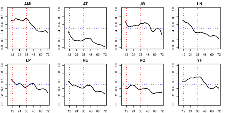
The X-axis is the number of months since release (i.e. horizon $\tau$). The Y-axis is the value of temporal quality. The solid lines are the moving average of $Q_{\omega=0.5}({\tau})$ with window size $k=5$. The dotted horizontal line at $0.5$ is the base line to assess VDM. Vertical lines are the marks of the horizons of $12^{th}$ and $36^{th}$ month.

Fig. 8: The trend of temporal quality $Q_{\omega=0.5}({\tau})$ of the VDMs in first 72 months.

Table VII reports the goodness-of-fit of existing VDMs on the largest horizons of browser releases, using the $\sf NVD$ data sets. In other words, we use following observed samples to evaluate all models:

$$\textit{OS}_{{\sf NVD}}=\left\{{\footnotesize\textsf{TS}}(r,{\sf NVD},{\tau}^{r}_{max})|r\in R\right\}$$

where $R$ is the set of all releases mentioned in Table VI. Table VII provides a view that previous studies often used to report the goodness-of-fit for their proposed models. To improve readability, we report the categorized goodness-of-fit based on the p-value (see II) instead of the raw p-values. In this table, we use a check mark (✓), a blank, and a cross ($\times$) to respectively indicate a Good Fit, an Inconclusive Fit, and a Not Fit. Cells are shaded accordingly to improve the visualization effect. The table shows that two models AT and RQ have a very high ratio of Not Fit ($0.9$ and $0.7$, respectively); whereas, all other models have their ratio of Not Fit less than 0.5. We should observe that this is a very large time interval and some systems have long gone into retirement. For example, FF v2.0 vulnerabilities are no longer sought by researchers. They are a byproduct of research on later versions.

To have a more realistic picture, we also study the temporal quality. The inconclusiveness contribution factor $\omega$ is set to $0.5$ as described in II. Fig. 8 exhibits the moving average (windows size $k=5$) of the $Q_{\omega}({\tau})$. The dotted vertical lines marks horizon $12$ (when software is young), and $36$ (when software is middle-age). We cut the temporal quality at horizon $72$ though we have more data for some systems (e.g., IE v4, FF v1.0). It is because that after 6 years software is very old, the vulnerability data reported for such releases might be not reliable, and might overfit the VDMs. The dotted horizon line at $0.5$ is used as a base line to assess VDMs.

Clearly from the temporal quality trends in Fig. 8 both AT and RQ models should be rejected since their temporal quality always sinks below the base line. Other models may be adequate when software is young (before 12 months). The AML and LN models look better than other models in this respect.

When software is middle-age (between 12 and 36 months), the AML model is still relatively good. JW and YF improve when approaching month $36^{th}$ though JW get worse after month $12^{th}$. The quality of both LN and LP worsen after month $12^{th}$, and sink below the base line when approaching month $36^{th}$. RE is almost below the base line after month $15^{th}$. Hence, in the middle-age period, AML, JW, and YF models may turn to be adequate; LN and LP are deteriorating but might be still considered adequate; whereas RE should clearly be rejected.

When software is old (36+ months), AML, JW, and YF deteriorate and go below the base line at month $48^{th}$ (approximately); other models also collapse below the base line.

Fig. 9 summarizes the distribution of VDM temporal quality in three period: software is young (before 12 moths), software is middle-age (13 to 36 months), and software is old (37 to 72 months). The red horizonal line at $0.5$ is the base line. We additionally colour these box plots according to the comparison between the corresponding distribution and the base line as follows:

• white: the distribution is significantly greater than the base line;

• dark gray: the distribution is significantly less than the base line (we should reject the models outright);

• gray: the distribution is not statistically different from the base line.

The box plots clearly confirm our observation in Fig. 8. Both AT and RE models are all significantly below the base line. AML, JW, and YF modes are significantly above the base line when software is young and middle age, and not statistically different from the base line when software is old. LN and LP models are significantly greater than the base line when software is young, but they deteriorate for middle-age software, and significantly collapse below the base line for old software.

In summary, our quality analysis shows that:

• AT and RQ models should be rejected.

• All other models may be adequate when software is young. Only s-shape models (i.e. AML, YW, YF) might be adequate when software is middle-age.

• No model is good when the software is too old.

Table VII: A potentially misleading results of overfitting VDMs in the largest horizon of browser releases, using $\sf NVD$ data sets

The goodness of fit of a VDM is based on p-value in the $\chi^{2}$ test. $\textit{p-value}<0.05$: not fit ($\times$), $\textit{p-value}\geq 0.80$: good fit (✓), and inconclusive fit (blank) otherwise. It is calculated over the entire lifetime.

	Firefox								Chrome												IE					Safari
	1	1.5	2	3	3.5	3.6	4	5	1	2	3	4	5	6	7	8	9	10	11	12	4	5	6	7	8	1	2	3	4	5
AML	$\times$	$\times$		$\times$	✓				✓		$\times$				$\times$		✓			$\times$	✓		$\times$		✓	$\times$				✓
AT	$\times$	$\times$	$\times$	$\times$	$\times$	$\times$			$\times$	$\times$	$\times$	$\times$	$\times$	$\times$	$\times$	$\times$	$\times$	$\times$	$\times$		$\times$	$\times$	$\times$	$\times$	$\times$	$\times$	$\times$	$\times$	$\times$
JW	$\times$	$\times$	✓	✓	✓	✓	✓		$\times$	$\times$	$\times$	$\times$			✓	✓					$\times$	✓	$\times$	✓		$\times$	$\times$	$\times$	$\times$	$\times$
LN	$\times$	$\times$		$\times$			✓		$\times$	$\times$	$\times$	$\times$								$\times$	$\times$	$\times$	$\times$	✓		$\times$	$\times$	$\times$	$\times$
LP	$\times$	$\times$	✓	✓	✓	✓	✓		$\times$	$\times$	$\times$	$\times$	$\times$				$\times$				$\times$	✓	$\times$	$\times$	✓	$\times$	$\times$	$\times$	$\times$
RE	$\times$	$\times$	✓	✓	✓	✓	✓		$\times$	$\times$	$\times$	$\times$	$\times$				$\times$				$\times$	✓	$\times$	$\times$	✓	$\times$	$\times$	$\times$	$\times$
RQ	$\times$	$\times$	$\times$	$\times$	$\times$		✓		$\times$	$\times$	$\times$					$\times$	$\times$	$\times$	$\times$	$\times$	$\times$	$\times$	$\times$	$\times$	✓	$\times$	$\times$	$\times$	$\times$	$\times$
YF	$\times$	$\times$	✓	✓	✓	✓	✓		✓	✓	✓	✓	✓	✓	✓		$\times$				✓	✓	✓	$\times$	✓	$\times$	$\times$	$\times$	$\times$

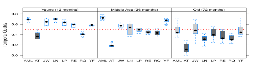
A horizonal line at value of $0.5$ is used as the base line to justify temporal quality. Box plots are coloured with respect to the comparison between the corresponding distribution and the base line: white - significantly above the base line, gray - no statistical difference, dark gray - significantly below the base line (i.e. rejected).

Fig. 9: The temporal quality distribution of each VDM in different periods of software lifetime.

5.2.2 Predictability Analysis for VDMs

From the previous quality analysis, AT and RQ models are low quality, and they should not be considered for all periods of software lifetime. Hence, we exclude these models from the predictability analysis. Furthermore, since no model is good when software is too old, we analyze the predictability of these models only for the first $36$ months since the release of a software. This period is still a large time if we consider that most recent releases live less than a year.

Fig. 10 reports the moving average (windows size equals $5$) for the trends of VDMs’ predictability along horizons in different prediction time spans. The dotted horizonal line at value of $0.5$ is the base line to assess the predictability of VDMs (as same as the temporal quality of VDMs).

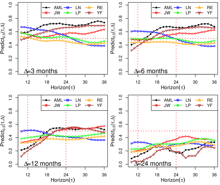
A horizonal line at value of $0.5$ is the base line to assess the predictability.

Fig. 10: The predictability of VDM in different prediction time spans ($\Delta$).

When the prediction time span is short ($3$ months), the predictability of LN, AML, JW, and LP models is above the base line for young software ($12$ months). When software is approaching month $24^{th}$, though decreasing the predictability of LN is still above the base line, but goes below the base line after month $24^{th}$. The LP model is no different with the base line before month $24^{th}$, but then also goes below the base line. In contrast, the predictability of AML, YF and JW are improving with age. They are all above the base line until the end of the study period (month $36^{th}$. Therefore, only s-shape models (AML, YF, and JW) may be adequate for middle-age software.

For the medium prediction time span of 6 months, only the LN model may be adequate (above the base line) when software is young, but becomes inadequate (below the base line) after month $24^{th}$. In the meanwhile S-shape models are inadequate for young software, but are improving quickly later. They may be all adequate after month $18^{th}$ and keep this performance until the end of the study period.

When the prediction time span is long (i.e. 12 months), all models (except LN) sink below the base line for young software. The LN model is not significantly different from the base line. In other words, no model could be adequate for young software in this prediction time span. After month $18^{th}$, the AML model goes above the base line, and after month $24^{th}$, all s-shape models are above the base line. Hence they may be all adequate. Their performances are somewhat unchanged for the remain period.

When the prediction time span is very long (i.e. 24 months) no model is good enough as all models sink below the base line.

In summary, our predictability analysis shows that:

• For a short prediction time span (i.e. 3 months), the predictability of LN, AML, and LP models may be adequate for young software. Hence they could be considered for the scenario Plan for short-term support. When software is approaching middle-age, s-shape models (AML, JW, YF) are better than others.

• For a medium (i.e. 6 months) and long (i.e. 12 month) prediction time spans, only the predictability of the LN model may be adequate for young software. And therefore this model could be appropriate the purpose of the scenarios Upgrade of keep and Plan for long-term support. When software is approaching middle-age, only s-shape models (AML, JW, YF) may be adequate and might be considered for planning the long-term support and for studying historical trends (i.e. scenario Historic analysis).

• For a very long prediction time span (i.e. 24 months), no model has a good enough predictability.

5.3 Comparison of Existing VDMs

The comparison between VDMs follows II. Instead of reporting tables of p-values, we visualize the comparison result in terms of directed graphs where nodes represent models, and connections represent the order relationship between models.

Fig. 11 summarizes the comparison results between models in different settings of horizons ($\tau$) and prediction time spans ($\Delta$). A directed connection from two models determines that the source model is better than the target model in terms of either predictability, or quality, or both. The line style of the connection depended on the following rules:

• Solid line: the predictability and quality of the source is significantly better than the target’s.

• Dashed line: the predictability of the source is significantly better than the target.

• Dotted line: the quality of the source is significantly better than the target.

By term significantly, we means the p-value of the corresponding one-side Wilcoxon rank-sum test is less than the significance level. We apply the Bonferroni correction to control the multi comparison problem, hence the significance level is: $\alpha=0.05/5=0.01$.

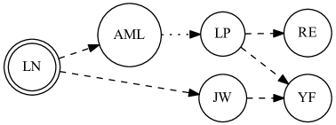
(a) Young software, short term prediction (${\tau}=6..12,\Delta=3$)

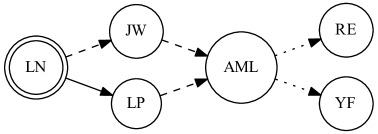
(b) Young software, medium term prediction (${\tau}=6..12,\Delta=6$)

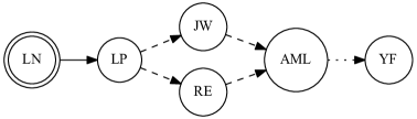
(c) Young software, 1 year prediction (${\tau}=6..12,\Delta=12$)

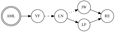
(d) Middle-age software, short term prediction (${\tau}=12..24,\Delta=03$)

(e) Middle-age software, 1 year prediction (${\tau}=12..24,\Delta=12$)

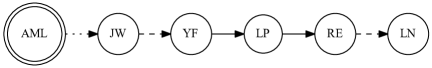
(f) Old software, 1 year prediction
(${\tau}=24..36,\Delta=12$)

A directed connection from two nodes determines that the source model is better than the target one with respect to their predictability (dashed line), or their quality (dotted line), or both (solid line). A double cirlce marks the best model. RQ and AT are not shown as they are the worst models.

Fig. 11: The comparison results among VDMs in some usage scenarios.

Table VIII: Suggested models for different usage scenarios.

	Observation	Prediction
Scenario	Period	Time Span	Model(s)
Plan for short-term support	6–12	3	LN
	12–24	3	AML
Plan for long-term support	6–12	12	LN
	12–24	12	AML
Upgrade or keep	6–12	6	LN
Historic analysis	24–36	12	AML

Note: the unit is month.

According to the figure, Table VIII suggests model(s) for different usage scenario described in the criteria II (see Table II).

In short, when software is young, the LN model is the most appropriate choice. This is because the vulnerability discovery is linear. When software is approaching middle-age, the AML model becomes superior.

6 Threats to Validity

Construct validity includes threats affecting the way we collect vulnerability data and the way we generate VDM curves with respect to the collected data. Following threats in this category are identified:

• Bugs in data collector. Most of vulnerability data are available in HTML pages. We have developed a web crawler to extract interesting feature from HTML page, and also XML data. The employed technique is as same as the one discussed in [14]. The crawler might be buggy and could generate errors in data collection. To minimize such impact, we have tested the crawler many times before collecting the data. Then by randomly checking the collected data, when an error is found we corrected the corresponding bug in the crawler and recollected the data.

• Bias in bug-to-nvd linking scheme. While collecting data for $\sf Advice.Nbug$, we apply some heuristic rules to link a $\sf bug$ to an $\sf NVD$ entry based on the relative position in the MFSA report. We manually checked many links for the relevant connection between bug reports and NVD entries. All checked links were found to be consistent. Some errors might still creep in this case.

• Bias in bug-affects-version identification. We do not have a complete assurance that a security bug affects to which versions. Consequently, we assume that a bug affects all versions mentioned in the linked $\sf NVD$. This might overestimate the number of bugs in each version. To mitigate the problem, we estimate the latest release that a bug might impact, and filter all vulnerable releases after this latest. Such estimation is done thank to the mining technique discussed in [21]. We further discuss these types of errors in NVD in [16]. These errors only affect the fitness of models over the long term so only valuations after the $24$ or $36$ months might be affected.

• Error in curve fitting. From the collected vulnerability, we estimate the parameters of VDMs by using the Nonlinear Least-Square technique implemented in R (nls() function). This might not produce the most optimal solution and may impact the goodness-of-fit of VDMs. To mitigate this issue, we additionally employed a commercial tool i.e. CurveExpert Pro to cross check the goodness-of-fit in many cases. The results have shown that there is no difference between R and CurveExpert.

Internal validity concerns the causal relationship between the collected data and the conclusion drawn in our study. Here, we have identified the following threats that might bias our conclusion.

• Bias in statistics tests. Our conclusions are based on statistics tests. These tests have their own assumptions. Choosing tests whose assumptions are violated might end up with wrong conclusions. To reduce the risk we carefully analyzed the assumptions of the tests to make sure no unwarranted assumption was present. We did not apply any tests with normality assumptions since the distribution of vulnerabilities is not normal.

External validity is the extent to which our conclusion could be generalized to other scenarios. Our experiment is based on the vulnerability data of some major releases of the four most popular browsers covering almost all market shares. Therefore we can be quite confident about our conclusion for browsers in general. However, it does not mean that our conclusion is valid for other types of application such as operating systems. Such validity requires extra experiments.

7 Related Work

Anderson [5] proposed a VDM (a.k.a. Anderson Thermodynamic, AT) based on reliability growth models, in which the probability of a security failure at time $t$, when $n$ bugs have been removed, is in inverse ratio to $t$ for alpha testers. This probability is even harder for beta testers, $\lambda$ times more than alpha testers. However, he did not conduct any experiment to validate the proposed model. Our results show that this model is not appropriate. This is a first evidence that reliability and security obey different laws.

Rescorla [19] also proposed two mathematical models, called Linear model (a.k.a Rescorla Quadratic, RQ) and Exponential model (a.k.a Rescorla Exponential, RE). He has performed an experiment on four versions of different operation systems (i.e. Windows NT 4.0, Solaris 2.5.1, FreeBSD 4.0 and RedHat 7.0). In all cases, the goodness-of-fit of these two models were inconclusive since their p-value ranged from $0.167$ to $0.589$. Rescorla discussed many shortcomings of NVD, but his study heavily relied on it nonetheless.

Alhazmi and Malaiya [1] proposed another VDM inspired by s-shape logistic model, called Alhazmi Malaiya Logistic (AML). The intuition behind the model is to divide the discovery process into three phases: learning phase, linear phase and saturation phase. In the first phase, people need some time to study the software, so less vulnerabilities are discovered. In the second phase, when people get deeper knowledge of the software, much more vulnerabilities are found. In the final phase, since the software is out of date, people may lose interest in finding new vulnerabilities. So cumulative vulnerabilities tend to stable. In [1], the authors validated their proposal against several versions of Windows (i.e. Win 95/98/NT4.0/2K) and Linux (i.e. RedHat Linux 6.1, 7.1). Their model fitted Win 95 very well (p-value $\approx 1$), and Win NT4.0 (p-value = $0.923$). For other versions, their own validation showed that the AML model was inconclusive (i.e. the p-value ranged from $0.054$ to $0.317$).

In another work, Alhazmi and Malaiya [3] compared their proposed model with Rescorla’s [19] (RE, RQ) and Anderson’s [5] (AT) on Windows 95/XP and Linux RedHat Linux 6.2, Fedora. The result shows that their logistic model has a better goodness-of-fit than others. For Windows 95 and Linux 6.2, as the vulnerabilities distribute along s-shape-like curves, only AML is able to fit it (p-value=1), whereas all other models fail to match the data (p-value $\leq 0.05$). For Windows XP, the story is different. RQ turns to be the best one with p-value$=0.97$, while AML poorly match the data (p-value=$0.147$).

Woo et al [22] carried out an experiment with AML model on three browsers IE, Firefox and Mozilla. However, it is unclear which versions of these browsers were analyzed. Most likely, they did not distinguish between versions. As discussed in section §3 (e.g., 2), this could largely bias their final result. In their experiment, IE has not been fitted, Firefox was fairly fitted, and Mozilla was good fitted. From this result, we could not conclude any thing about the performance of AML. In another experiment, Woo et al [23] validated AML against two web servers: Apache and IIS. Also, they did not distinguish between versions of Apache and IIS. In this experiment, AML has demonstrated a very good performance on vulnerability data (p-value $=1$).

Kim et al [11] introduced the Multiple-Version Discovery Model (MVDM) which is the generalization of AML. The MVDM separated the cumulative vulnerabilities of a version into several fragments where the first fragment captured the vulnerabilities affecting this version and past versions, and the other fragments are the shared vulnerabilities of this version and future versions. The MVDM basically is the weighted aggregation of individual AML model in these fragments. The weights are determined by the ratios of shared code between this version and future ones. The goodness-of-fit of MVDM has been compared with AML in two versions of Apache and two version of MySQL. As the result, both AML and MVDM were well fitted against the data ($\textit{p-value}\geq 0.99$). MVDM might be better but the difference was quite negligible.

Joh et al [10] proposed a VDM based on the Weibull distribution. The proposed model was also compared with the AML model in two versions of Windows (XP, Server 2007) and two versions of Linux (RedHat Linux and RedHat Enterprise Linux). In that evaluation, the goodness-of-fit of the proposed model was compared with the AML model.

Younis et al [24] exploited the Folded distribution to model the discovery of vulnerabilities. The authors also compared the proposed model with the AML model in different types of application (Windows 7, OSX 5.0, Apache 2.0.x, and IE8). The reported results showed that the new model is better than the AML in the cases when the learning phase is not present.

8 Conclusion

Vulnerability discovery models have the potential to help us in predicting future vulnerability trends. Such predictions could help individuals and companies to adapt their software upgrade and patching schedule. However, we have not seen any method to systematically assess these models. Hence, in this work we have proposed an empirical methodology for VDM validation. The methodology is built upon the analyses on the goodness-of-fit, and the predictability of VDM at several time points during the software lifetime. These analyses rely on two quantitative metrics: quality and predictability.

We have applied this methodology to conduct an empirical experiment to assess eight VDMs (i.e. AML, AT, LN, JW, LP, RE, RQ, and YF) based on the vulnerability data of 30 major releases of four web browsers: IE, Firefox, Chrome, and Safari. Our experiment has revealed that:

• AT and RQ models should be rejected since their quality is not good enough.

• For young software, the quality of all other models may be adequate. Only the predictability of LN is good enough for short (i.e. 3 months and medium (i.e. 6 months) prediction time spans, other models however is not good enough for latter time span.

• For middle-age software, only s-shape models (i.e. AML, JW, and YF) may be adequate in terms of both quality and predictability.

• For old software, no model is good enough.

• No model is good enough for predicting results for a very long period (i.e. 24 months in the future).

In conclusion, for young releases of browsers ($6$ – $12$ months old) it is better to use a linear model to estimate the vulnerabilities in the next $3$ – $6$ months. For middle age browsers ($12$ – $24$ months) it is better to use an s-shape logistic model.

In future, it is interesting to replicate our experiment in other kinds of software, for instance operating systems and server-side applications. Based on that, a more comprehensive assessment about the VDMs will be more solid.

A replication guide of this work could be found online at https://wiki.science.unitn.it/security/doku.php?id=vulnerability_discovery_models. Also, you can find all required materials (e.g., tools, scripts, and data) to rerun the experiment.

Viet Hung Nguyen He is a PhD student in computer science at University of Trento, Italy under the supervision of professor Fabio Massacci since November 2009. He received his MSc and BEng in computer science and computer engineering in 2007 and 2003. Currently, his main interest is the correlation of vulnerability evolution and software code base evolution.

Fabio Massacci

References

- [1] Omar Alhazmi and Yashwant Malaiya. Modeling the vulnerability discovery process. In Proceedings of the 16th IEEE International Symposium on Software Reliability Engineering (ISSRE’05), pages 129–138, 2005.
- [2] Omar Alhazmi and Yashwant Malaiya. Measuring and enhancing prediction capabilities of vulnerability discovery models for Apache and IIS HTTP servers. In Proceedings of the 17th IEEE International Symposium on Software Reliability Engineering (ISSRE’06), pages 343–352, 2006.
- [3] Omar Alhazmi and Yashwant Malaiya. Application of vulnerability discovery models to major operating systems. IEEE Transactions on Reliability, 57(1):14–22, 2008.
- [4] Omar Alhazmi, Yashwant Malaiya, and Indrajit Ray. Security vulnerabilities in software systems: A quantitative perspective. In Sushil Jajodia and Duminda Wijesekera, editors, Data and Applications Security XIX, volume 3654 of LNCS, pages 281–294. 2005.
- [5] Ross Anderson. Security in open versus closed systems - the dance of Boltzmann, Coase and Moore. In Proceedings of Open Source Software: Economics, Law and Policy, 2002.
- [6] William A. Arbaugh, William L. Fithen, and John McHugh. Windows of vulnerability: A case study analysis. IEEE Computer, 33(12):52–59, 2000.
- [7] Algirdas Avizienis, Jean-Claude Laprie, Brian Randell, and Carl Landwehr. Basic concepts and taxonomy of dependable and secure computing. IEEE Transactions on Dependable and Secure Computing, 1(1):11–33, 2004.
- [8] Mark Dowd, John McDonald, and Justin Schuh. The art of software security assessment. Addision-Wesley publications, 2007.
- [9] Philip J. Fleming and John J. Wallace. How not to lie with statistics: the correct way to summarize benchmark results. Communication of the ACM, 29(3):218–221, 1986.
- [10] HyunChul Joh, Jinyoo Kim, and Yashwant Malaiya. Vulnerability discovery modeling using Weibull distribution. In Proceedings of the 19th IEEE International Symposium on Software Reliability Engineering (ISSRE’08), pages 299–300, 2008.
- [11] Jinyoo Kim, Yashwant Malaiya, and Indrajit Ray. Vulnerability discovery in multi-version software systems. In Proceeding of the 10th IEEE International Symposium on High Assurance Systems Engineering, pages 141–148, 2007.
- [12] Ivan Victor Krsul. Software Vulnerability Analysis. PhD thesis, Purdue University, 1998.
- [13] Fabio Massacci, Stephan Neuhaus, and Viet Hung Nguyen. After-life vulnerabilities: A study on firefox evolution, its vulnerabilities and fixes. In Proceedings of the 2011 Engineering Secure Software and Systems Conference (ESSoS’11), 2011.
- [14] Fabio Massacci and Viet Hung Nguyen. Which is the right source for vulnerabilities studies? an empirical analysis on mozilla firefox. In Proceedings of the International ACM Workshop on Security Measurement and Metrics (MetriSec’10), 2010.
- [15] Steve McKillup. Statistics Explained: An Introductory Guide for Life Scientists. Cambridge University Press, 2005.
- [16] Viet Hung Nguyen and Fabio Massacci. The (un) reliability of nvd vulnerable versions data: an empirical experiment on google chrome vulnerabilities. In Proceeding of the 8th ACM Symposium on Information, Computer and Communications Security (ASIACCS’13), 2013.
- [17] NIST/SEMATECH. e-Handbook of Statistical Methods, 2012. http://www.itl.nist.gov/div898/handbook/.
- [18] Andy Ozment. Improving vulnerability discovery models: Problems with definitions and assumptions. In Proceedings of the 3rd Workshop on Quality of Protection, 2007.
- [19] Eric Rescorla. Is finding security holes a good idea? IEEE Security and Privacy, 3(1):14–19, 2005.
- [20] Fred B. Schneider. Trust in cyberspace. National Academy Press, 1991.
- [21] Jacek Sliwerski, Thomas Zimmermann, and Andreas Zeller. When do changes induce fixes? In Proceedings of the 2nd International Working Conference on Mining Software Repositories MSR(’05), pages 24–28, May 2005.
- [22] Sung-Whan Woo, Omar Alhazmi, and Yashwant Malaiya. An analysis of the vulnerability discovery process in web browsers. In Proceedings of the 10th IASTED International Conferences Software Engineering and Applications, 2006.
- [23] Sung-Whan Woo, HyunChul Joh, Omar Alhazmi, and Yashwant Malaiya. Modeling vulnerability discovery process in Apache and IIS HTTP servers. Computer & Security, 30(1):50 – 62, 2011.
- [24] Awad Younis, HyunChul Joh, and Yashwant Malaiya. Modeling learningless vulnerability discovery using a folded distribution. In Proceeding of the Internaltional Conference Security and Management (SAM’11), pages 617–623, 2011.