Relative Observability of Discrete-Event Systems and its Supremal Sublanguages

Abstract

We identify a new observability concept, called relative observability, in supervisory control of discrete-event systems under partial observation. A fixed, ambient language is given, relative to which observability is tested. Relative observability is stronger than observability, but enjoys the important property that it is preserved under set union; hence there exists the supremal relatively observable sublanguage of a given language. Relative observability is weaker than normality, and thus yields, when combined with controllability, a generally larger controlled behavior; in particular, no constraint is imposed that only observable controllable events may be disabled. We design new algorithms which compute the supremal relatively observable (and controllable) sublanguage of a given language, which is generally larger than the normal counterparts. We demonstrate the new observability concept and algorithms with a Guideway and an AGV example.

I Introduction

In supervisory control of discrete-event systems, partial observation arises when the supervisor does not observe all events generated by the plant [1, 2]. This situation is depicted in Fig. 1(a), where ${\bf G}$ is the plant with closed behavior $L({\bf G})$ and marked behavior $L_{m}({\bf G})$, $P$ is a natural projection that nulls unobservable events, and $V^{o}$ is the supervisor under partial observation. The fundamental observability concept is identified in [3, 4]: observability and controllability of a language $K\subseteq L_{m}({\bf G})$ is necessary and sufficient for the existence of a nonblocking supervisor $V^{o}$ synthesizing $K$. The observability property is not, however, preserved under set union, and hence there generally does not exist the supremal observable and controllable sublanguage of a given language.

The normality concept studied in [3, 4] is stronger than observability but algebraically well-behaved: there always exists the supremal normal and controllable sublanguage of a given language. The supremal sublanguage may be computed by methods in [5, 6]; also see a coalgebra-based method in [7]. Normality, however, imposes the constraint that controllable events cannot be disabled unless they are observable [1, Section 6.5]. This constraint might result in overly conservative controlled behavior.

To fill the gap between observability and normality, in this paper we identify a new concept called relative observability. For a language $K\subseteq L_{m}({\bf G})$, we fix an ambient language $\overline{C}$ such that $\overline{K}\subseteq\overline{C}\subseteq L({\bf G})$ (here $\overline{\ \cdot\ }$ denotes prefix closure, defined in Section II). It is relative to the ambient language $\overline{C}$ that observability of $K$ is tested. We prove that relative observability is stronger than the observability in [3, 4] (strings in $\overline{C}-\overline{K}$, if any, need to be tested), weaker than normality (unobservable controllable events may be disabled), and preserved under set union. Hence, there exists the supremal relatively observable and controllable sublanguage of a given language, which is generally larger than the supremal normal counterpart, and may be synthesized by a nonblocking supervisor. This result is useful in practical situations where there may be not enough sensors available for all controllable events, or it might be too costly to have all; the result may also help deal with the practical issue of sensor failures.

We then design new algorithms to compute the supremal sublanguages, capable of keeping track of the ambient language. These results are demonstrated with a Guideway and an AGV example in Section V, providing quantitative evidence of improvements by relative observability as compared to normality. Note that in the special case $\overline{C}=\overline{K}$, relative observability coincides with observability for the given $K$. The difference, however, is that when a family of languages is considered, the ambient $\overline{C}$ in relative observability is held fixed. It is this feature that renders relative observability algebraically well-behaved.

Figure 1: Supervisory control under partial observation. $L({\bf G})$ is the closed behavior of the plant, $P$ a natural projection modeling the observation channel, $V^{o}$ the supervisor under partial observation. In (b), $L(V/{\bf G})$ is the closed-loop controlled behavior with full observation.

Another special case is when the ambient $\overline{C}=L({\bf G})$. As suggested by Fig. 1(a), $L({\bf G})$ is a natural choice for the ambient language because strings in $L({\bf G})$ are observed through the channel $P$. When control is in place, a more reasonable choice for the ambient $\overline{C}$ is $L(V/{\bf G})$, the optimal nonblocking controlled behavior under full observation, since any string in $L({\bf G})-L(V/{\bf G})$ is effectively prohibited by control; see Fig. 1(b). With $\overline{C}=L(V/{\bf G})$, the supremal relatively observable and controllable sublanguage is generally larger than the supremal normal counterpart; this is illustrated by empirical studies on a Guideway and an AGV example in Section V.

In [8], Takai and Ushio reported an observability property, formulated in a state-based form, which is preserved under a union operation of “strict subautomata”. This operation does not correspond to language union. It was shown that the (marked) language of “the supremal subautomaton” with the proposed observability is generally larger than the supremal normal counterpart. As will be illustrated by examples, their observability property and our relative observability do not generally imply each other. In the Guideway example in Subsection V-A, we present a case where our algorithm computes a strictly larger controlled behavior.

We note that, for prefix-closed languages, several procedures are developed to compute a maximal observable and controllable sublanguage, e.g. [9, 10, 11, 12, 13]. Those procedures are not, however, applicable to non-closed languages, because the resulting supervisor may be blocking. In addition, the observability concept has been extended to coobservability in decentralized supervisory control (e.g. [14, 15]), state-based observability (e.g. [16, 17]), timed observability in real-time discrete-event systems (e.g. [18, 19]), and optimal supervisory control with costs [20]. Observability and normality have also been used in modular, decentralized, and coordination control architectures (e.g. [21, 22, 23]). In the present paper, we focus on centralized, monolithic supervision for untimed systems in the Ramadge-Wonham language framework [1, 24], and leave those extensions of relative observability for future research.

The rest of this paper is organized as follows. Section II introduces the relative observability concept, and establishes its properties. Section III presents an algorithm to compute the supremal relatively observable sublanguage of a given language, and Section IV combines relative observability and controllability to generate controlled behavior generally larger than the normality counterpart. Section V demonstrates the results with a Guideway and an AGV example. Finally Section VI states our conclusions.

II Relative Observability

The plant to be controlled is modeled by a generator

$$\textbf{G}=(Q,\Sigma,\delta,q_{0},Q_{m})$$ (1)

where $Q$ is the finite state set; $q_{0}\in Q$ is the initial state; $Q_{m}\subseteq Q$ is the subset of marker states; $\Sigma$ is the finite event set; $\delta:Q\times\Sigma\rightarrow Q$ is the (partial) state transition function. In the usual way, $\delta$ is extended to $\delta:Q\times\Sigma^{*}\rightarrow Q$, and we write $\delta(q,s)!$ to mean that $\delta(q,s)$ is defined. The closed behavior of G is the language

$$L(\textbf{G}):=\{s\in\Sigma^{*}|\delta(q_{0},s)!\}\subseteq\Sigma^{*};$$ (2)

the marked behavior is

$$L_{m}(\textbf{G}):=\{s\in L(\textbf{G})|\delta(q_{0},s)\in Q_{m}\}\subseteq L(\textbf{G}).$$ (3)

A string $s_{1}$ is a prefix of a string $s$, written $s_{1}\leq s$, if there exists $s_{2}$ such that $s_{1}s_{2}=s$. The (prefix) closure of $L_{m}(\textbf{G})$ is $\overline{L_{m}(\textbf{G})}:=\{s_{1}\in\Sigma^{*}\ |\ (\exists s\in L_{m}(\textbf{G}))s_{1}\leq s\}$. In this paper we assume $\overline{L_{m}(\textbf{G})}=L(\textbf{G})$; namely G is nonblocking.

For partial observation, let the event set $\Sigma$ be partitioned into $\Sigma_{o}$, the observable event subset, and $\Sigma_{uo}$, the unobservable subset (i.e. $\Sigma=\Sigma_{o}\dot{\cup}\Sigma_{uo}$). Bring in the natural projection $P:\Sigma^{*}\rightarrow\Sigma_{o}^{*}$ defined according to

$$\begin{split}P(\epsilon)&=\epsilon,\ \ \epsilon\mbox{ is the empty string;}\\ P(\sigma)&=\left\{\begin{array}[]{ll}\epsilon,&\hbox{if $\sigma\notin\Sigma_{o}$,}\\ \sigma,&\hbox{if $\sigma\in\Sigma_{o}$;}\end{array}\right.\\ P(s\sigma)&=P(s)P(\sigma),\ \ s\in\Sigma^{*},\sigma\in\Sigma.\end{split}$$ (4)

In the usual way, $P$ is extended to $P:Pwr(\Sigma^{*})\rightarrow Pwr(\Sigma^{*}_{o})$, where $Pwr(\cdot)$ denotes powerset. Write $P^{-1}:Pwr(\Sigma^{*}_{o})\rightarrow Pwr(\Sigma^{*})$ for the inverse-image function of $P$. Given two languages $L_{i}\subseteq\Sigma^{*}_{i}$, $i=1,2$, their synchronous product is $L_{1}||L_{2}:=P_{1}^{-1}L_{1}\cap P_{2}^{-1}L_{2}\subseteq(\Sigma_{1}\cup\Sigma_{2})^{*}$, where $P_{i}:(\Sigma_{1}\cup\Sigma_{2})^{*}\rightarrow\Sigma^{*}_{i}$.

Observability of a language is a familiar concept [3, 4]. Now fixing a sublanguage $C\subseteq L_{m}(\textbf{G})$, we introduce relative observability which sets $\overline{C}\subseteq L(\textbf{G})$ to be the ambient language in which observability is tested.

Definition 1.

Let $K\subseteq C\subseteq L_{m}(\textbf{G})$. We say $K$ is relatively observable with respect to $\overline{C}$, G, and $P$, or simply $\overline{C}$-observable, if for every pair of strings $s,s^{\prime}\in\Sigma^{*}$ that are lookalike under $P$, i.e. $P(s)=P(s^{\prime})$, the following two conditions hold:

$$(i)\ (\forall\sigma\in\Sigma)\ s\sigma\in\overline{K},s^{\prime}\in\overline{C},s^{\prime}\sigma\in L(\textbf{G})\Rightarrow s^{\prime}\sigma\in\overline{K}$$ (5)

$$(ii)\ s\in K,s^{\prime}\in\overline{C}\cap L_{m}(\textbf{G})\Rightarrow s^{\prime}\in K$$ (6)

Note that a pair of lookalike strings $(s,s^{\prime})$ trivially satisfies (5) and (6) if either $s$ or $s^{\prime}$ does not belong to the ambient $\overline{C}$. For a lookalike pair $(s,s^{\prime})$ both in $\overline{C}$, relative observability requires that (i) $s$ and $s^{\prime}$ have identical one-step continuations, if allowed in $L(\textbf{G})$, with respect to membership in $\overline{K}$; and (ii) if each string is in $L_{m}(\textbf{G})$ and one actually belongs to $K$, then so does the other. A graphical explanation of the concept is given in Fig. 2.

Figure 2: Verification of relative observability of $K$ requires checking all three lookalike strings $s,s^{\prime},s^{\prime\prime}$ in the ambient language $\overline{C}$, while verification of observability of $K$ requires checking only $s,s^{\prime}$ in $\overline{K}$. For $K$ to be $\overline{C}$-observable, condition (5) requires $s^{\prime\prime}\sigma\notin L(\textbf{G})$, and condition (6) requires $s^{\prime\prime}\notin L_{m}(\textbf{G})$.

If $\overline{C_{1}}\subseteq\overline{C_{2}}\subseteq L({\bf G})$ are two ambient languages, it follows easily from Definition 1 that $\overline{C_{2}}$-observability implies $\overline{C_{1}}$-observability. Namely, the smaller the ambient language, the weaker the relative observability. In the special case where the ambient $\overline{C}=\overline{K}$, Definition 1 becomes the standard observability [3, 4] for the given $K$. This immediately implies

Proposition 1.

If $K\subseteq C$ is $\overline{C}$-observable, then $K$ is also observable.

The reverse statement need not be true. An example is provided in Fig. 3, which displays an observable language that is not relatively observable.

Figure 3: $L_{m}(\textbf{K})$ is observable but not relatively observable. In $L(\textbf{K})$ the only lookalike string pair is $(\alpha,\alpha\beta)$; it is easily verified that $L_{m}(\textbf{K})$ is observable. To see that $L_{m}(\textbf{K})$ is not $\overline{C}$-observable, let $s=\epsilon$ and $s^{\prime}=\beta$ ($\notin L(\textbf{K})$). We have $s\alpha\in L(\textbf{K})$, $s^{\prime}\alpha\in\overline{C}=L(\textbf{G})$, but $s^{\prime}\alpha\notin L(\textbf{K})$. This violates (5). Also consider $s=\alpha\beta$ and $s^{\prime}=\beta\alpha$ ($\notin L_{m}(\textbf{K})$). We have $s\in L_{m}(\textbf{K})$, $s^{\prime}\in\overline{C}\cap L_{m}(\textbf{G})$, but $s^{\prime}\notin L_{m}(\textbf{K})$. This violates (6).

An important way in which relative observability differs from observability is the exploitation of a fixed ambient $\overline{C}\subseteq L(\textbf{G})$. Let $K_{i}\subseteq C$, $i=1,2$. For (standard) observability of each $K_{i}$, one checks lookalike string pairs only in $\overline{K_{i}}$, ignoring all candidates permitted by the other language. Observability of $K_{i}$ is in this sense ‘myopic’, and consequently, both $K_{i}$ being observable need not imply that their union $K_{1}\cup K_{2}$ is observable. The fixed ambient language $\overline{C}$, by contrast, provides a ‘global reference’: no matter which $K_{i}$ one checks for relative observability, all lookalike string pairs in $\overline{C}$ must be considered. This more stringent requirement renders relative observability algebraically well-behaved, as we will see in Subsection II-B. Before that, we first show the relation between relative observability and normality [3, 4].

II-A Relative observability is weaker than normality

In this subsection, we show that relative observability is weaker than normality, a property that is also preserved by set unions [3, 4]. A sublanguage $K\subseteq C$ is $(L_{m}(\textbf{G}),P)$-normal if

$$K=P^{-1}PK\cap L_{m}(\textbf{G}).$$ (7)

If, in addition, $\overline{K}$ is $(L(\textbf{G}),P)$-normal, then no string in $\overline{K}$ may exit $\overline{K}$ via an unobservable transition [1, Section 6.5]. This means, when control is present, that one cannot disable any unobservable, controllable events. Relative observability, by contrast, does not impose this restriction, i.e. one may exercise control over unobservable events.

Proposition 2.

If $K\subseteq C$ is $(L_{m}(\textbf{G}),P)$-normal and $\overline{K}$ is $(L(\textbf{G}),P)$-normal, then $K$ is $\overline{C}$-observable.

Proof. Let $s,s^{\prime}\in\Sigma^{*}$ and $Ps=Ps^{\prime}$. We must show that both (5) and (6) hold for $K$.

For (5), let $\sigma\in\Sigma$, $s\sigma\in\overline{K}$, $s^{\prime}\in\overline{C}$, and $s^{\prime}\sigma\in L(\textbf{G})$; it will be shown that $s^{\prime}\sigma\in\overline{K}$. From $s\sigma\in\overline{K}$ we have

$$P(s\sigma)\in P\overline{K} \Rightarrow P(s)P(\sigma)\in P\overline{K}$$

$$\Rightarrow P(s^{\prime})P(\sigma)\in P\overline{K}$$

$$\Rightarrow P(s^{\prime}\sigma)\in P\overline{K}$$

$$\Rightarrow s^{\prime}\sigma\in P^{-1}P\overline{K}$$

Hence $s^{\prime}\sigma\in P^{-1}P\overline{K}\cap L(\textbf{G})=\overline{K}$ by normality of $\overline{K}$.

For (6), let $s\in K$, $s^{\prime}\in\overline{C}\cap L_{m}(\textbf{G})$; we will prove $s^{\prime}\in K$. That $s\in K$ implies $Ps\in PK$; thus $Ps^{\prime}\in PK$, i.e. $s^{\prime}\in P^{-1}PK$. Therefore $s^{\prime}\in P^{-1}PK\cap L_{m}(\textbf{G})=K$ by normality of $K$. $\square$

In the proof we note that $\overline{K}$ being $(L(\textbf{G}),P)$-normal implies condition (i) of relative observability, and independently $K$ being $(L_{m}(\textbf{G}),P)$-normal implies condition (ii). The reverse statement of Proposition 2 need not be true; an example is displayed in Fig. 4.

In Section V, we will see examples where the supremal relatively observable controlled behavior is strictly larger than the supremal normal counterpart. This is due exactly to the distinction as to whether or not one may disable controllable events that are unobservable.

Figure 4: $L_{m}(\textbf{K})$ is relatively observable but not normal. In $L(\textbf{K})$ all three strings are lookalike; it is easily verified that $L_{m}(\textbf{K})$ is $\overline{C}$-observable. To see that $L_{m}(\textbf{K})$ is not $(L_{m}(\textbf{G}),P)$-normal, calculate $P^{-1}PL_{m}(\textbf{K})=P^{-1}(\epsilon)=\Sigma^{*}$. Thus $P^{-1}PL_{m}(\textbf{K})\cap L_{m}(\textbf{G})=L_{m}(\textbf{G})\varsupsetneqq L_{m}(\textbf{K})$. A similar calculation yields that $L(\textbf{K})$ is not $(L(\textbf{G}),P)$-normal.

Figure 5: Comparison with [8]. In (a), $L_{m}(\textbf{K})$ is $L({\bf C})$-observable; but ${\bf K}$ is not observable in the sense of [8], because state pair $(q,q^{\prime})$ with $q$ in ${\bf K}$ and $q^{\prime}$ not in ${\bf K}$ violates the observability condition in [8]. In (b), K is observable in the sense of [8]; but $L_{m}(\textbf{K})$ is not $L({\bf C})$-observable, because $\gamma\sigma\in L(\textbf{K})$, $\beta\gamma\in L(\textbf{C})$, $\beta\gamma\sigma\in L(\textbf{G})$, $P(\gamma)=P(\beta\gamma)$, but $\beta\gamma\sigma\notin L(\textbf{K})$.

We note that [8] reported an observability property which is also weaker than normality. The observability condition in [8] is formulated in a generator form, which is preserved under a particularly-defined union operation of “strict subautomata”. This automata union does not correspond to language/set union, and hence the reported observability might not be preserved under set union. In addition, the observability condition in [8] requires checking all state pairs $(q,q^{\prime})$ reached by lookalike strings in the whole state set $Q$ of G. This corresponds to checking all lookalike string pairs in $L(\textbf{G})$; in this sense, our relative observability is weaker with the ambient language $\overline{C}\subseteq L(\textbf{G})$. One such example is provided in Fig. 5(a). This point is also illustrated, when combined with controllability, in the Guideway example in Section V-A. However, the reverse case is also possible, as displayed in Fig. 5(b).

II-B The supremal relatively observable sublanguage

First, an arbitrary union of relatively observable languages is again relatively observable.

Proposition 3.

Let $K_{i}\subseteq C$, $i\in I$ (some index set), be $\overline{C}$-observable. Then $K=\bigcup\{K_{i}\ |\ i\in I\}$ is also $\overline{C}$-observable.

Proof. Let $s,s^{\prime}\in\Sigma^{*}$ and $Ps=Ps^{\prime}$. We must show that both (5) and (6) hold for $K$.

For (5), let $\sigma\in\Sigma$, $s\sigma\in\overline{K}$, $s^{\prime}\in\overline{C}$, and $s^{\prime}\sigma\in L(\textbf{G})$; it will be shown that $s^{\prime}\sigma\in\overline{K}$. Since $\overline{K}=\overline{\bigcup K_{i}}=\bigcup\overline{K_{i}}$, there exists $j\in I$ such that $s\sigma\in\overline{K_{j}}$. But $K_{j}$ is $\overline{C}$-observable, which yields $s^{\prime}\sigma\in\overline{K_{j}}$. Hence $s^{\prime}\sigma\in\bigcup\overline{K_{i}}=\overline{K}$.

For (6), let $s\in K$, $s^{\prime}\in\overline{C}\cap L_{m}(\textbf{G})$; we will prove $s^{\prime}\in K$. That $s\in K=\bigcup K_{i}$ implies that there exists $j\in I$ such that $s\in K_{j}$. Since $K_{j}$ is $\overline{C}$-observable, we have $s^{\prime}\in K_{j}$. Therefore $s^{\prime}\in\bigcup K_{i}=K$.

$\square$

Figure 6: The intersection of two relatively observable languages is not relatively observable. It is easily verified that both $K_{1}$ and $K_{2}$ are $\overline{C}$-observable. Their intersection $K$, however, is not: let $s=\epsilon$ and $s^{\prime}=\alpha$; then $Ps=Ps^{\prime}$, $s\sigma\in\overline{K}$, $s^{\prime}\in\overline{C}$, $s^{\prime}\sigma\in L({\bf G})$, but $s^{\prime}\sigma\notin\overline{K}$. Thus condition (5) of relative observability is violated.

While relative observability is closed under arbitrary unions, it is generally not closed under intersections. Fig. 6 provides an example for which the intersection of two $\overline{C}$-observable sublanguages is not $\overline{C}$-observable.

Whether or not $K\subseteq C$ is $\overline{C}$-observable, write

$$\mathcal{O}(K,C):=\{K^{\prime}\subseteq K\ |\ K^{\prime}\mbox{ is $\overline{C}$-observable}\}$$ (8)

for the family of $\overline{C}$-observable sublanguages of $K$. The discussion above on unions and intersections of relatively observable languages shows that $\mathcal{O}(K,C)$ is an upper semilattice of the lattice of sublanguages of $K$, with respect to the partial order ($\subseteq$). Note that the empty language $\emptyset$ is trivially $\overline{C}$-observable, thus a member of $\mathcal{O}(K,C)$. By Proposition 3 we derive that $\mathcal{O}(K,C)$ has a unique supremal element sup$\mathcal{O}(K,C)$ given by

$$\mbox{sup}\mathcal{O}(K,C):=\bigcup\{K^{\prime}\ |\ K^{\prime}\in\mathcal{O}(K,C)\}.$$ (9)

This is the supremal $\overline{C}$-observable sublanguage of $K$. We state these important facts about $\mathcal{O}(K,C)$ in the following.

Theorem 1.

Let $K\subseteq C$. The set $\mathcal{O}(K,C)$ is nonempty, and contains its supremal element sup$\mathcal{O}(K,C)$ in (9).

For (9), of special interest is when the ambient language is set to equal $\overline{K}$:

$$\mbox{sup}\mathcal{O}(K):=\bigcup\{K^{\prime}\ |\ K^{\prime}\in\mathcal{O}(K)\},\ \mbox{ where }\mathcal{O}(K):=\{K^{\prime}\subseteq K\ |\ K^{\prime}\mbox{ is $\overline{K}$-observable}\}$$ (10)

Proposition 4.

For $K\subseteq C\subseteq L_{m}({\bf G})$, it holds that $\mbox{sup}\mathcal{O}(K,C)\subseteq\mbox{sup}\mathcal{O}(K)$.

Proof. For each $K^{\prime}\subseteq K$, it follows from Definition 1 that if $K^{\prime}$ is $\overline{C}$-observable, then $K^{\prime}$ is also $\overline{K}$-observable. Hence $\mathcal{O}(K,C)\subseteq\mathcal{O}(K)$, and sup$\mathcal{O}(K,C)\subseteq$ sup$\mathcal{O}(K)$. $\square$

Proposition 4 shows that sup$\mathcal{O}(K)$ is the largest relatively observable sublanguage of $K$, given all choices of the ambient language. It is therefore of particular interest in characterizing and computing sup$\mathcal{O}(K)$. We do so in the next section using a generator-based approach.

III Generator-Based Computation of sup$\mathcal{O}(K)$

In this section we design an algorithm that computes the supremal relatively observable sublanguage sup$\mathcal{O}(K)$ of a given language $K$. This algorithm has two new mechanisms that distinguish it from those computing the supremal normal sublanguage (e.g. [5, 6, 7]): First, compared to [5, 6, 7], the algorithm embeds a more intricate, ‘fine-grained’ procedure (to be stated precisely below) for processing transitions of the generators involved; this new procedure is needed because relative observability is weaker than normality, and thus generally requires fewer transitions to be removed. Second, the algorithm keeps track of strings in the ambient language $\overline{K}$, as required by the relative observability conditions; by contrast, this is simply not an issue in [5, 6, 7] for the normality computation.

III-A Setting

Consider a nonblocking generator $\textbf{G}=(Q,\Sigma,\delta,q_{0},Q_{m})$ as in (1) with regular languages $L_{m}(\textbf{G})$ and $L(\textbf{G})$, and a natural projection $P:\Sigma^{*}\rightarrow\Sigma^{*}_{o}$ with $\Sigma_{o}\subseteq\Sigma$. Let $K$ be an arbitrary regular sublanguage of $L_{m}(\textbf{G})$. Then $K$ can be represented by a finite-state generator ${\bf K}=(Y,\Sigma,\eta,y_{0},Y_{m})$; that is, $L_{m}({\bf K})=K$ and $L({\bf K})=\overline{K}$. For simplicity we assume ${\bf K}$ is nonblocking, i.e. $\overline{L_{m}(\textbf{K})}=L(\textbf{K})$. Denote by $n,m$ respectively the number of states and transitions of ${\bf K}$, i.e.

$$\begin{split}&n:=|Y|\\ &m:=|\eta|=|\{(y,\sigma,\eta(y,\sigma))\in Y\times\Sigma\times Y\ |\ \eta(y,\sigma)!\}|.\end{split}$$ (11)

We introduce

Assumption 1. $(\forall s,t\in L({\bf K}))\ \eta(y_{0},s)=\eta(y_{0},t)\Rightarrow\delta(q_{0},s)=\delta(q_{0},t)$.

If the given ${\bf K}$ does not satisfy Assumption 1, form the following synchronous product ([1, 2])

$${\bf K}||{\bf G}=(Y\times Q,\Sigma,\eta\times\delta,(y_{0},q_{0}),Y_{m}\times Q_{m})$$ (12)

where $\eta\times\delta:Y\times Q\times\Sigma\rightarrow Y\times Q$ is given by

$$(\eta\times\delta)\big{(}(y,q),\sigma\big{)}=\left\{\begin{array}[]{ll}\big{(}\eta(y,\sigma),\delta(q,\sigma)\big{)},&\hbox{if $\eta(y,\sigma)!$ \& $\delta(q,\sigma)!$;}\\ \mbox{undefined},&\hbox{otherwise.}\end{array}\right.$$

It is easily checked (e.g. [2, Section 2.3.3]) that $L({\bf K}||{\bf G})=L({\bf K})\cap L({\bf G})=L({\bf K})$, $L_{m}({\bf K}||{\bf G})=L_{m}({\bf K})\cap L_{m}({\bf G})=L_{m}({\bf K})$, and for every $s,t\in L({\bf K}||{\bf G})$ if $(\eta\times\delta)\big{(}(y_{0},q_{0}),s\big{)}=(\eta\times\delta)\big{(}(y_{0},q_{0}),t\big{)}$, then $\delta(q_{0},s)=\delta(q_{0},t)$. Namely ${\bf K}||{\bf G}$ satisfies Assumption 1. Therefore, replacing ${\bf K}$ by the synchronous product ${\bf K}||{\bf G}$ always makes Assumption 1 hold.

Now if for some $s\in L({\bf K})$ a string $Ps\in PL({\bf K})$ is observed, then the “uncertainty set” of states which $s$ may reach in ${\bf K}$ is

$$U(s):=\{\eta(y_{0},s^{\prime})\ |\ s^{\prime}\in L({\bf K}),Ps^{\prime}=Ps\}\subseteq Y.$$ (13)

If two strings have the same uncertainty set, then the following is true.

Lemma 1.

Let $s,t\in L({\bf K})$ be such that $U(s)=U(t)$. If $s^{\prime}\in L({\bf K})$ looks like $s$, i.e. $Ps^{\prime}=Ps$, then there exists $t^{\prime}\in L({\bf K})$ such that $Pt^{\prime}=Pt$ and $\eta(y_{0},t^{\prime})=\eta(y_{0},s^{\prime})$.

Proof. Since $s^{\prime}\in L({\bf K})$ and $Ps^{\prime}=Ps$, by (13) we have $\eta(y_{0},s^{\prime})\in U(s)$. Then it follows from $U(s)=U(t)$ that $\eta(y_{0},s^{\prime})\in U(t)$, and hence there exists $t^{\prime}\in L({\bf K})$ such that $Pt^{\prime}=Pt$ and $\eta(y_{0},t^{\prime})=\eta(y_{0},s^{\prime})$. $\square$

We further adopt

Assumption 2.

$$(\forall s,t\in L({\bf K}))\ \eta(y_{0},s)=\eta(y_{0},t)\Rightarrow U(s)=U(t).$$ (14)

Assumption 2 requires that any two strings reaching the same state of ${\bf K}$ must have the same uncertainty set. This requirement is equivalent to the “normal automaton” condition in [5, 8], which played a key role in their algorithms. In case the given ${\bf K}$ does not satisfy (14), a procedure is presented in [8, Appendix A] which makes Assumption 2 hold. Essentially, the procedure consists of two steps: first, construct a deterministic generator ${\bf PK}$ with event set $\Sigma_{o}$ obtained by the subset construction such that $L_{m}({\bf PK})=PL_{m}({\bf K})$ and $L({\bf PK})=PL({\bf K})$ (e.g. [1, Section 2.5]). The subset construction ensures that if two strings $Ps,Pt$ reach the same state in ${\bf PK}$, then $U(s)=U(t)$. The state size of ${\bf PK}$ is at worst exponential in that of ${\bf K}$. Second, form the synchronous product ${\bf K}||{\bf PK}$ as in (12), so that $L({\bf K}||{\bf PK})=L({\bf K})\cap P^{-1}PL({\bf K})=L({\bf K})$ and $L_{m}({\bf K}||{\bf PK})=L_{m}({\bf K})\cap P^{-1}PL_{m}({\bf K})=L_{m}({\bf K})$. Therefore, replacing ${\bf K}$ by ${\bf K}||{\bf PK}$ always makes Assumption 2 hold. Like Assumption 1, Assumption 2 entails no loss of generality.

Let Assumptions 1 and 2 hold. We present an algorithm which produces a finite sequence of generators

$$({\bf K}=){\bf K}_{0},\ \ {\bf K}_{1},\ \ \cdots,\ \ {\bf K}_{N}$$ (15)

with ${\bf K}_{i}=(Y_{i},\Sigma,\eta_{i},y_{0},Y_{m,i})$, $i\in[0,N]$, and a corresponding finite descending chain of languages

$$(L_{m}({\bf K})=)L_{m}({\bf K}_{0})\supseteq L_{m}({\bf K}_{1})\supseteq\cdots\supseteq L_{m}({\bf K}_{N})$$

such that $L_{m}({\bf K}_{N})=$ sup$\mathcal{O}(K)$ in (9) with the ambient language $\overline{K}$. If $K$ is observable (in the standard sense), then $N=0$.

III-B Observational consistency

Given ${\bf K}_{i}=(Y_{i},\Sigma,\eta_{i},y_{0},Y_{m,i})$, $i\in[0,N]$, suppose $\overline{L_{m}({\bf K}_{i})}=L({\bf K}_{i})$, namely ${\bf K}_{i}$ is nonblocking. We need to check whether or not $L_{m}({\bf K}_{i})$ is $\overline{K}$-observable. To this end, we introduce a generator-based condition, called observational consistency. We proceed in two steps. First, let

$${\bf\tilde{K}}_{i}=(\tilde{Y}_{i},\Sigma,\tilde{\eta}_{i},y_{0},Y_{m,i})$$ (16)

where $\tilde{Y}_{i}=Y_{i}\cup\{y_{d}\}$, with the dump state $y_{d}\notin Y_{i}$, and $\tilde{\eta}_{i}$ is an extension of $\eta_{i}$ which is fully defined on $\tilde{Y}_{i}\times\Sigma$, i.e.

$$\tilde{\eta}_{i}(y_{0},s)=\left\{\begin{array}[]{ll}\eta_{i}(y_{0},s),&\hbox{if $s\in L({\bf K}_{i})$;}\\ y_{d},&\hbox{if $s\in\Sigma^{*}-L({\bf K}_{i})$.}\end{array}\right.$$ (19)

Clearly, the closed and marked languages of ${\bf\tilde{K}}_{i}$ satisfy $L({\bf\tilde{K}}_{i})=\Sigma^{*}$ and $L_{m}({\bf\tilde{K}}_{i})=L_{m}({\bf K}_{i})$.

Second, for each $s\in\Sigma^{*}$ define a set $T_{i}(s)$ of state pairs in G and ${\bf\tilde{K}}_{i}$ by

$$T_{i}(s):=\{(q,y)\in Q\times\tilde{Y}_{i}\ |\ (\exists s^{\prime})Ps^{\prime}=Ps,q=\delta(q_{0},s^{\prime}),y=\tilde{\eta}_{i}(y_{0},s^{\prime}),\eta(y_{0},s^{\prime})!\}.$$ (20)

Thus, a pair $(q,y)\in T_{i}(s)$ if $q\in Q$ and $y\in\tilde{Y}_{i}$ are reached by a common string $s^{\prime}$ that looks like $s$, and this $s^{\prime}$ is in $L(\textbf{K})$, namely the ambient $\overline{K}$, because $\eta(y_{0},s^{\prime})!$. This $\eta(y_{0},s^{\prime})!$ is the key to tracking strings in the ambient $\overline{K}$.

Remark 1. If one aims to compute $\mbox{sup}\mathcal{O}(K,C)$ in (9) instead of the largest $\mbox{sup}\mathcal{O}(K)$ in (10) (largest in the sense of Proposition 4), for some ambient language $C$ satisfying $K\subseteq C\subseteq L_{m}({\bf G})$, then replace $T_{i}(s)$ in (20) by

$$T^{C}_{i}(s):=\{(q,y)\in Q\times\tilde{Y}_{i}\ |\ (\exists s^{\prime})Ps^{\prime}=Ps,q=\delta(q_{0},s^{\prime}),y=\tilde{\eta}_{i}(y_{0},s^{\prime}),\eta^{C}(y_{0},s^{\prime})!\}.$$ (21)

where $\eta^{C}$ is the transition function of the generator ${\bf C}$ with $L_{m}({\bf C})=C$ and $L({\bf C})=\overline{C}$. The rest follows similarly by using $T^{C}_{i}(s)$.

Definition 2.

We say that $T_{i}(s)$ is observationally consistent (with respect to ${\bf G}$ and ${\bf\tilde{K}}_{i}$) if for all $(q,y),(q^{\prime},y^{\prime})\in T_{i}(s)$ there holds

$$(\forall\sigma\in\Sigma)\ \tilde{\eta}_{i}(y,\sigma)\neq y_{d},\delta(q^{\prime},\sigma)!\Rightarrow\tilde{\eta}_{i}(y^{\prime},\sigma)\neq y_{d}$$ (22)

$$q^{\prime}\in Q_{m},y\in Y_{m,i}\Rightarrow y^{\prime}\in Y_{m,i}.$$ (23)

Note that if $T_{i}(s)$ has only one element, then it is trivially observationally consistent. Let

$$\mathcal{T}_{i}:=\{T_{i}(s)\ |\ s\in\Sigma^{*},|T_{i}(s)|\geq 2\}.$$ (24)

Then $|\mathcal{T}_{i}|\leq 2^{|Q|\cdot(|\tilde{Y}_{i}|)}\leq 2^{|Q|\cdot(n+1)}$, which is finite. The following result states that checking $\overline{K}$-observability of $L_{m}({\bf K}_{i})$ is equivalent to checking observational consistency of all state pairs in each of the $T_{i}$ occurring in $\mathcal{T}_{i}$.

Lemma 2.

$L_{m}({\bf K}_{i})$ is $\overline{K}$-observable if and only if for every $T\in\mathcal{T}_{i}$, $T$ is observationally consistent with respect to ${\bf G}$ and ${\bf\tilde{K}}_{i}$.

Proof. (If) Let $s,s^{\prime}\in\Sigma^{*}$ and $Ps=Ps^{\prime}$. We must show that both (5) and (6) hold for $L_{m}({\bf K}_{i})$.

For (5), let $\sigma\in\Sigma$, $s\sigma\in L({\bf K}_{i})$, $s^{\prime}\in\overline{K}$, and $s^{\prime}\sigma\in L(\textbf{G})$; it will be shown that $s^{\prime}\sigma\in L({\bf K}_{i})$. According to (20) and (19), the two state pairs $(\delta(q_{0},s),\tilde{\eta}_{i}(y_{0},s)),(\delta(q_{0},s^{\prime}),\tilde{\eta}_{i}(y_{0},s^{\prime}))$ belong to $T(s)$. Now $s\sigma\in L({\bf K}_{i})$ implies $\tilde{\eta}_{i}(\tilde{\eta}_{i}(y_{0},s),\sigma)\neq y_{d}$ (by (19)), and $s^{\prime}\sigma\in L(\textbf{G})$ implies $\delta(\delta(q_{0},s^{\prime}),\sigma)!$. Since $T(s)$ is observationally consistent, by (22) we have $\tilde{\eta}_{i}(\tilde{\eta}_{i}(y_{0},s^{\prime}),\sigma)\neq y_{d}$. Then it follows from (19) that $s^{\prime}\sigma\in L({\bf K}_{i})$.

For (6), let $s\in L_{m}({\bf K}_{i})$, $s^{\prime}\in\overline{K}\cap L_{m}(\textbf{G})$; we will prove $s^{\prime}\in L_{m}({\bf K}_{i})$. Again $(\delta(q_{0},s),\tilde{\eta}_{i}(y_{0},s))$, $(\delta(q_{0},s^{\prime}),\tilde{\eta}_{i}(y_{0},s^{\prime}))\in T(s)$ according to (20) and (19). Now $s\in L_{m}({\bf K}_{i})=L_{m}({\bf\tilde{K}}_{i})$ implies $\tilde{\eta}_{i}(y_{0},s)\in Y_{m,i}$, and $s^{\prime}\in L_{m}(\textbf{G})$ implies $\delta(q_{0},s^{\prime})\in Q_{m}$. Since $T(s)$ is observationally consistent, by (23) we have $\tilde{\eta}_{i}(y_{0},s^{\prime})\in Y_{m,i}$, i.e. $s^{\prime}\in L_{m}({\bf\tilde{K}}_{i})=L_{m}({\bf K}_{i})$.

(Only if) Let $T\in\mathcal{T}_{i}$, and $(q,y),(q^{\prime},y^{\prime})\in T$ corresponding respectively to some $s$ and $s^{\prime}$ with $Ps=Ps^{\prime}$. We must show that both (22) and (23) hold.

For (22), let $\sigma\in\Sigma$, $\tilde{\eta}_{i}(y,\sigma)\neq y_{d}$, and $\delta(q^{\prime},\sigma)!$. It will be shown that $\tilde{\eta}_{i}(y^{\prime},\sigma)\neq y_{d}$. Now $(q,y)\in T$ and $\tilde{\eta}_{i}(y,\sigma)\neq y_{d}$ imply $s\sigma\in L({\bf K}_{i})$ (by (19)); $(q^{\prime},y^{\prime})\in T$ and $\delta(q^{\prime},\sigma)!$ imply $s^{\prime}\in\overline{K}$ and $s^{\prime}\sigma\in L(\textbf{G})$. Since $L_{m}({\bf K}_{i})$ is $\overline{K}$-observable, by (5) we have $s^{\prime}\sigma\in L({\bf K}_{i})$, and therefore $\tilde{\eta}_{i}(y^{\prime},\sigma)\neq y_{d}$.

Finally for (23), let $y\in Y_{m,i}$, $q^{\prime}\in Q_{m}$. We will show $y^{\prime}\in Y_{m,i}$. From $(q,y)\in T$ and $y\in Y_{m,i}$, $s\in L_{m}({\bf\tilde{K}}_{i})=L_{m}(\textbf{K}_{i})$; from $(q^{\prime},y^{\prime})\in T$ and $q^{\prime}\in Q_{m}$, $s^{\prime}\in\overline{K}\cap L_{m}(\textbf{G})$. Since $L_{m}({\bf K}_{i})$ is $\overline{K}$-observable, by (6) we have $s^{\prime}\in L_{m}(\textbf{K}_{i})=L_{m}({\bf\tilde{K}}_{i})$, i.e. $y^{\prime}\in Y_{m,i}$. $\square$

If there is $T\in\mathcal{T}_{i}$ that fails to be observationally consistent, then there exist state pairs $(q,y),(q^{\prime},y^{\prime})\in T$ such that either (22) or (23) or both are violated. Define two sets $R_{T}$ and $M_{T}$ as follows:

$$R_{T} :=\bigcup_{\sigma\in\Sigma}\{(y,\sigma,\eta_{i}(y,\sigma))\ |\ \eta_{i}(y,\sigma)!\ \&\ (\exists(q^{\prime},y^{\prime})\in T)(\delta(q^{\prime},\sigma)!\ \&\ \tilde{\eta}_{i}(y^{\prime},\sigma)=y_{d})\}$$ (25)

$$M_{T} :=\{y\in Y_{m,i}\ |\ (\exists(q^{\prime},y^{\prime})\in T)\ q^{\prime}\in Q_{m}\ \&\ y^{\prime}\notin Y_{m,i}\}$$ (26)

Thus $R_{T}$ is a collection of transitions of ${\bf K}_{i}$, each having corresponding state pairs $(q,y),(q^{\prime},y^{\prime})\in T$ that violate (22), while $M_{T}$ is a collection of marker states of ${\bf K}_{i}$, each having corresponding state pairs that violate (23). To make $T$ observationally consistent, all transitions in $R_{T}$ have to be removed, and all states in $M_{T}$ unmarked. These constitute the main steps in the algorithm below.

III-C Algorithm

We now present an algorithm which computes sup$\mathcal{O}(K)$ in (9).

Algorithm 1: Input $\textbf{G}=(Q,\Sigma,\delta,q_{0},Q_{m})$, $\textbf{K}=(Y,\Sigma,\eta,y_{0},Y_{m})$, and $P:\Sigma^{*}\rightarrow\Sigma^{*}_{o}$.

1. Set $\textbf{K}_{0}=(Y_{0},\Sigma,\eta_{0},y_{0},Y_{m,0})=\textbf{K}$, namely $Y_{0}=Y$, $Y_{m,0}=Y_{m}$, and $\eta_{0}=\eta$.

2. For $i\geq 0$, calculate $\mathcal{T}_{i}$ as in (24) and (20) based on G, K, ${\bf\tilde{K}}_{i}=(\tilde{Y}_{i},\Sigma,\tilde{\eta}_{i},y_{0},Y_{m,i})$ in (16), and $P$.

3. For each $T\in\mathcal{T}_{i}$, check if $T$ is observationally consistent with respect to ${\bf G}$ and ${\bf\tilde{K}}_{i}$ (i.e. check if conditions (22) and (23) are satisfied for all $(q,y),(q^{\prime},y^{\prime})\in T$):

If every $T\in\mathcal{T}_{i}$ is observationally consistent with respect to ${\bf G}$ and ${\bf\tilde{K}}_{i}$, then go to Step 4 below. Otherwise, let

$$R_{i} :=\bigcup_{T\in\mathcal{T}_{i}}R_{T},\ \mbox{where $R_{T}$ is defined in (\ref{eq:RT})}$$ (27)

$$M_{i} :=\bigcup_{T\in\mathcal{T}_{i}}M_{T},\ \mbox{where $M_{T}$ is defined in (\ref{eq:MT})}$$ (28)

and set

$$\eta^{\prime}_{i} :=\eta_{i}-R_{i}$$ (29)

$$Y^{\prime}_{m,i} :=Y_{m,i}-M_{i}.$$ (30)

Let $\textbf{K}_{i+1}=(Y_{i+1},\Sigma,\eta_{i+1},y_{0},Y_{m,i+1})=$ trim$((Y_{i},\Sigma,\eta^{\prime}_{i},y_{0},Y^{\prime}_{m,i}))$, where trim$(\cdot)$ removes all non-reachable and non-coreachable states and corresponding transitions of the argument generator. Now advance $i$ to $i+1$, and go to Step 2.

4. Output $\textbf{K}_{N}:={\bf K}_{i}$.

Algorithm 1 has two new mechanisms as compared to those computing the supremal normal sublanguage (e.g. [5, 6, 7]). First, the mechanism of the normality algorithms in [5, 6, 7] is essentially this: If a transition $\sigma$ is removed from state $y$ of ${\bf\tilde{K}}_{i}$ reached by some string $s$, then remove $\sigma$ from all states $y^{\prime}$ reached by a lookalike string $s^{\prime}$, i.e. $Ps=Ps^{\prime}$. (In fact if $\sigma$ is unobservable, then all the states $y$ and $y^{\prime}$ as above are removed.) This (all or nothing) mechanism generally causes, however, ‘overkill’ of transitions (i.e. removing more transitions than necessary) in our case of relative observability, because the latter is weaker than normality and allows more permissive behavior. Indeed, some $\sigma$ transitions at states $y^{\prime}$ as above may be preserved without violating relative observability. Corresponding to this feature, Algorithm 1 employs a new, fine-grained mechanism: in Step 3, remove as in (29) only those transitions of ${\bf\tilde{K}}_{i}$ that violate the relative observability conditions. Moreover, the second new mechanism of Algorithm 1 is that it keeps track of strings in the ambient language $L({\bf K})$ at each iteration by computing $\mathcal{T}_{i}$ in (24) with $T_{i}$ in (20) in Step 2 above. It is these two new mechanisms that enable Algorithm 1 to compute the supremal relatively observable sublanguage sup$\mathcal{O}(K)$ in (9).

The two new mechanisms of Algorithm 1 come with an extra computational cost as compared to the normality algorithms in [5, 6, 7]. The extra cost is precisely the computation of $\mathcal{T}_{i}$ in (24), which is in the worst case exponential in $n$ because $|\mathcal{T}_{i}|\leq 2^{(n+1)|Q|}$. While complexity is an important issue for practical computation, we shall leave for future research the problem of finding more efficient alternatives to Algorithm 1. In our empirical study in Section V, the supremal relatively observable sublanguages corresponding to generators with state size of the order $10^{3}$ are computed reasonably fast by Algorithm 1 (see the AGV example).

Algorithm 1 terminates in finite steps: in (29), the set $R_{T}$ of transitions for every (observationally inconsistent) $T\in\mathcal{T}_{i}$ is removed; in (30), the set $M_{T}$ of marker states for every (observationally inconsistent) $T\in\mathcal{T}_{i}$ is unmarked. At each iteration of Algorithm 1, if at Step 3 there is an observationally inconsistent $T$, then at least one of the two sets $R_{i}$ in (27) and $M_{i}$ in (28) is nonempty. Therefore at least one transition is removed and/or one marker state is unmarked. As initially in $\textbf{K}_{0}=\textbf{K}$ there are $m$ transitions and $|Y_{m}|$ $(<n)$ marker states, Algorithm 1 terminates in at most $n+m$ iterations. The complexity of Algorithm 1 is $O((n+m)2^{(n+1)|Q|})$, because the search ranges $\mathcal{T}_{i}$ are such that $|\mathcal{T}_{i}|\leq 2^{(n+1)|Q|}$. Note that if ${\bf K}$ does not satisfy Assumption 2, we have to replace ${\bf K}$ by ${\bf K}||{\bf PK}$ and then the complexity of Algorithm 1 is $O((2^{n}+m)2^{(2^{n}+1)|Q|})$.

Note that from $\textbf{K}_{i}$ to $\textbf{K}_{i+1}$ in Step 3 above, for all $s,t\in\Sigma^{*}$ if $\eta_{i+1}(y_{0},s)!$, $\eta_{i+1}(y_{0},t)!$, then $\eta_{i}(y_{0},s)!$, $\eta_{i}(y_{0},t)!$, and

$$\eta_{i+1}(y_{0},s)=\eta_{i+1}(y_{0},t)\Rightarrow\eta_{i}(y_{0},s)=\eta_{i}(y_{0},t)$$ (31)

Now we state our main result.

Theorem 2.

Let Assumptions 1 and 2 hold. Then the output $\textbf{K}_{N}$ of Algorithm 1 satisfies $L_{m}(\textbf{K}_{N})=$ sup$\mathcal{O}(K)$, the supremal $\overline{K}$-observable sublanguage of $K$.

Figure 7: Generator ${\bf K^{\prime}}$ does not satisfy (14): strings $\alpha\beta$ and $\gamma\alpha$ both reach state $y_{1}$, but $U(\alpha\beta)=\{y_{1},y_{2},y_{3},y_{4}\}\supsetneqq U(\gamma\alpha)=\{y_{1},y_{4}\}$. Now $T(\alpha)$ is not observationally consistent; indeed, two state pairs $(q_{1},y_{1}),(q_{2},y_{2})\in T(\alpha)$ violate both (22) (for transition $\sigma$) and (23). Applying Algorithm 1 will remove $\sigma$ at $y_{1}$ and unmark $y_{1}$, which unintentionally removes string $\gamma\alpha\sigma$ and unmarks $\gamma\alpha$. These latter two strings, however, belong to the supremal $\overline{K^{\prime}}$-observable sublanguage. This undesirable situation is avoided in ${\bf K}$ where the strings $\alpha\beta$ and $\gamma\alpha$ are arranged to reach different states, and it is easily checked that ${\bf K}$ satisfies (14).

The condition (14) of Assumption 2 on ${\bf K}$ is important for Algorithm 1 to generate the supremal relatively observable sublanguage, because it avoids removing and/or unmarking a string which is not intended. An illustration is displayed in Fig. 7.

Figure 8: In ${\bf K}_{0}$, state pairs $(q_{1},y_{1}),(q_{2},y_{2})\in T(\alpha)$ are observationally consistent, while $(q_{2},y_{2}),(q_{4},y_{d})\in T(\alpha)$ are not ($y_{d}$ is the dump state): (22) is violated for transition $\beta$. Applying Algorithm 1 will remove $\beta$ at $y_{2}$, and the result is ${\bf K}_{1}$. In ${\bf K}_{1}$, state pairs $(q_{1},y_{1}),(q_{2},y_{2})\in T(\alpha)$ become observationally inconsistent: again (22) is violated for transition $\beta$. Algorithm 1 needs to be applied again to remove $\beta$ at $y_{1}$.

Note that removing a transition and/or unmarking a state may destroy observational consistency of other state pairs. Fig. 8 displays such an example. This implies that all state pairs need to be checked for observational consistency at each iteration of Algorithm 1.

In addition, just for checking $\overline{C}$-observability of a given language $K$, with $K\subseteq C$, a polynomial algorithm (see [2, Section 3.7], [26]) for checking (standard) observability may be adapted. Indeed, let ${\bf C}$ be a generator representing $C$, and instead of forming the synchronous product ${\bf G}||{\bf K}||{\bf K}$ as in [2, Section 3.7], we form ${\bf G}||{\bf C}||{\bf K}$; the rest is similar as may be easily confirmed.

Finally, we provide an example to illustrate the operations involved in Algorithm 1.

Example 1.

Figure 9: Example illustration of Algorithm 1. Events $\beta_{1},...,\beta_{5}$ are unobservable and $\alpha,\gamma,\sigma$ observable.

Consider generators ${\bf G}$ and ${\bf K}$ displayed in Fig. 9, where events $\beta_{1},...,\beta_{5}$ are unobservable and $\alpha,\gamma,\sigma$ observable. These events define a natural projection $P$. It is easily checked that Assumption 1 holds. Also, in ${\bf K}$, we have $U(\alpha)=U(\gamma)=\{y_{1},y_{7},y_{8},y_{9}\}$ and $U(\alpha\sigma)=U(\gamma\sigma)=\{y_{6},y_{11}\}$; thus ${\bf K}$ satisfies (14) and Assumption 2 holds.

Apply Algorithm 1 with inputs ${\bf G}$, ${\bf K}$, and the natural projection $P$. Set ${\bf K}_{0}={\bf K}$, and compute $\mathcal{T}_{0}=\{T_{1},T_{2},T_{3}\}$ with

$$T_{1} =\{(q_{0},y_{0}),(q_{2},y_{2}),(q_{3},y_{3}),(q_{4},y_{4}),(q_{5},y_{5})\}\ (=T(\epsilon))$$

$$T_{2} =\{(q_{1},y_{1}),(q_{7},y_{7}),(q_{8},y_{8}),(q_{9},y_{9})\}\ (=T(\alpha)=T(\gamma))$$

$$T_{3} =\{(q_{6},y_{6}),(q_{11},y_{11})\}\ (=T(\alpha\sigma)=T(\gamma\sigma)).$$

While $T_{1},T_{3}$ are observationally consistent with respect to ${\bf K}_{0}$, $T_{2}$ is not; indeed, $(q_{7},y_{7}),(q_{8},y_{8})$ violate (22) with event $\beta_{5}$. Thus $R_{0}=\{(y_{7},\beta_{5},y_{9})\}$ and $M_{0}=\emptyset$; the unobservable transition $(y_{7},\beta_{5},y_{9})$ is removed, which yields a trim generator ${\bf K}_{1}$ in Fig. 9.

The above is the first iteration of Algorithm 1. Next, compute $\mathcal{T}_{1}=\{T_{1},T_{2},T_{3},T_{4},T_{5}\}$ with

$$T_{1} =\{(q_{0},y_{0}),(q_{2},y_{2}),(q_{3},y_{3}),(q_{4},y_{4}),(q_{5},y_{5})\}\ (=T(\epsilon))$$

$$T_{2} =\{(q_{1},y_{1}),(q_{7},y_{7}),(q_{8},y_{8}),(q_{9},y_{d})\}\ (=T(\gamma))$$

$$T_{3} =\{(q_{1},y_{1}),(q_{7},y_{7}),(q_{8},y_{8}),(q_{9},y_{9}),(q_{9},y_{d})\}\ (=T(\alpha))$$

$$T_{4} =\{(q_{6},y_{d}),(q_{11},y_{d})\}\ (T(\gamma\sigma))$$

$$T_{5} =\{(q_{6},y_{d}),(q_{11},y_{11}),(q_{11},y_{d})\}\ (=T(\alpha\sigma)).$$

Note that $T(\alpha)\neq T(\gamma)$ and $T(\alpha\sigma)\neq T(\gamma\sigma)$ in ${\bf K}_{1}$, although $T(\alpha)=T(\gamma)$ and $T(\alpha\sigma)=T(\gamma\sigma)$ in ${\bf K}_{0}$. Now $T_{2}$,…,$T_{5}$ are all observationally inconsistent with respect to ${\bf K}_{1}$, and $R_{1}=\{(y_{1},\sigma,y_{6})\}$, $M_{1}=\{y_{11}\}$. Thus removing transition $(y_{1},\sigma,y_{6})$, unmarking $y_{11}$, and trimming the result yield ${\bf K}_{2}$ in Fig. 9. This finishes the second iteration of Algorithm 1.

Compute $\mathcal{T}_{3}=\{T_{1},T_{2}\}$ with

$$T_{1} =\{(q_{0},y_{0}),(q_{2},y_{d}),(q_{3},y_{3}),(q_{4},y_{4}),(q_{5},y_{5})\}\ (=T(\epsilon))$$

$$T_{2} =\{(q_{1},y_{1}),(q_{7},y_{7}),(q_{8},y_{8}),(q_{9},y_{d})\}\ (=T(\gamma)=T(\alpha)).$$

Here $T_{1}$ is not observationally consistent, and $R_{3}=\{(y_{0},\alpha,y_{1}),(y_{3},\alpha,y_{7}),(y_{5},\alpha,y_{8})\}$, $M_{3}=\emptyset$. Thus removing these three transitions and trimming the result yield ${\bf K}_{3}$ in Fig. 9. This is the third iteration of Algorithm 1. Now compute $\mathcal{T}_{4}=\{T_{1},T_{2}\}$ with

$$T_{1} =\{(q_{0},y_{0}),(q_{2},y_{d}),(q_{3},y_{d}),(q_{4},y_{4}),(q_{5},y_{5})\}\ (=T(\epsilon))$$

$$T_{2} =\{(q_{1},y_{1}),(q_{7},y_{7}),(q_{8},y_{8}),(q_{9},y_{d})\}\ (=T(\gamma)).$$

It is easily checked that both $T_{1}$ and $T_{2}$ are observationally consistent with respect to ${\bf K}_{3}$; by Lemma 2, $L_{m}({\bf K}_{3})$ is $L({\bf K})$-observable. Hence Algorithm 1 terminates after four iterations, and outputs ${\bf K}_{3}$. By Theorem 2, $L_{m}({\bf K}_{3})$ is in fact the supremal $L({\bf K})$-observable sublanguage of $L({\bf K})$. By contrast, the supremal normal sublanguage of $L({\bf K})$ is empty.

We now prove Theorem 2.

Proof of Theorem 2. We show $L_{m}(\textbf{K}_{N})=$ sup$\mathcal{O}(K)$. First, it is guaranteed by Algorithm 1 that for the output $\textbf{K}_{N}$, all the corresponding $T\in\mathcal{T}_{N}$ are observationally consistent; hence Lemma 2 implies that $L_{m}(\textbf{K}_{N})$ is $\overline{K}$-observable.

It remains to prove that if $K^{\prime}\in\mathcal{O}(K)$, then $K^{\prime}\subseteq L_{m}(\textbf{K}_{N})$. We proceed by induction on the iterations $i=0,1,2,...$ of Algorithm 1. Since $K^{\prime}\subseteq K=L_{m}(\textbf{K})$, we have $K^{\prime}\subseteq L_{m}(\textbf{K}_{0})$. Suppose now $K^{\prime}\subseteq L_{m}(\textbf{K}_{i})$; we show that $K^{\prime}\subseteq L_{m}(\textbf{K}_{i+1})$. Let $w\in K^{\prime}$; by hypothesis $w\in L_{m}(\textbf{K}_{i})$. It will be shown that $w\in L_{m}(\textbf{K}_{i+1})$ as well.

First, suppose on the contrary that $w\notin L({\bf K}_{i+1})$. Since $w\in L({\bf K}_{i})$, there exist $t\in\Sigma^{*}$ and $\sigma\in\Sigma$ such that $t\sigma\leq w$, $\eta_{i}(y_{0},t)=:y\in Y_{i}$, and $(y,\sigma,\eta_{i}(y,\sigma))\in R_{i}$ in (27). Then there is $T\in\mathcal{T}_{i}$ such that $(y,\sigma,\eta_{i}(y,\sigma))\in R_{T}$ in (25), and $T$ is not observationally consistent ((22) is violated). Since $K^{\prime}$ is $\overline{K}$-observable and $t\in\overline{K^{\prime}}$, Lemma 2 implies that $T(t)$ is observationally consistent, and thus $T(t)\neq T$.

Now let $s\in\Sigma^{*}$ be such that $s\neq t$, $\eta_{i}(y_{0},s)=\eta_{i}(y_{0},t)=y$, and $T(s)=T$. Then by (25) there exists $(q^{\prime},y^{\prime})\in T(s)$ such that $\delta(q^{\prime},\sigma)!$ and $\tilde{\eta}_{i}(y^{\prime},\sigma)=y_{d}$. Let $s^{\prime}\in L({\bf K}_{0})=L({\bf K})$ be such that $Ps=Ps^{\prime}$, $\delta(q_{0},s^{\prime})=q^{\prime}$, and $\tilde{\eta}_{i}(y_{0},s^{\prime})=y^{\prime}$. Whether or not $y^{\prime}=y_{d}$, there must exist $s^{\prime}_{1},u\in\Sigma^{*}$ such that $s^{\prime}_{1}u=s^{\prime}$, $\tilde{\eta}_{i}(y_{0},s^{\prime}_{1})\neq y_{d}$ (i.e. $\eta_{i}(y_{0},s^{\prime}_{1})!$), and the following is true: if $u=\epsilon$ then $\tilde{\eta}_{i}(y_{0},s^{\prime}_{1}\sigma)=y_{d}$; otherwise, for each $u_{1}\in\overline{\{u\}}-\{\epsilon\}$, $\tilde{\eta}_{i}(y_{0},s^{\prime}_{1}u_{1})=y_{d}$. We claim that $u\in\Sigma^{*}_{uo}$, i.e. an unobservable string. Otherwise, if there exist $u_{1}\leq u$ and $\alpha\in\Sigma_{o}$ such that $u_{1}\alpha\leq u$, then by $Ps=Ps^{\prime}$ there is $s_{1}\leq s$ such that $s_{1}\alpha\leq s$ and $Ps_{1}=P(s^{\prime}_{1}u_{1})$. Since $\tilde{\eta}_{i}(y_{0},s^{\prime}_{1}u_{1}\alpha)=y_{d}$, we have $(\eta_{j}(y_{0},s_{1}),\alpha,\eta_{j}(y_{0},s_{1}\alpha))\in R_{j}$ for some $j<i$. Hence $s\notin L({\bf K}_{i})$, which is contradicting our choice of $s$ that $\eta_{i}(y_{0},s)=\eta_{i}(y_{0},t)=y$.

Now $u\in\Sigma^{*}_{uo}$ and $s^{\prime}_{1}u=s^{\prime}$ imply $Ps^{\prime}_{1}=Ps^{\prime}=Ps$. Since $\eta_{i}(y_{0},s)=\eta_{i}(y_{0},t)=y$, by repeatedly using (31) we derive $\eta_{0}(y_{0},s)=\eta_{0}(y_{0},t)=y$. Then by Assumption 2 and Lemma 1, there exists $t^{\prime}\in L({\bf K}_{0})$ such that $Pt=Pt^{\prime}$ and $\eta_{0}(y_{0},t^{\prime})=\eta_{0}(y_{0},s^{\prime}_{1})$. Thus $\eta_{0}(y_{0},t^{\prime}u)=\eta_{0}(y_{0},s^{\prime}_{1}u)$. It then follows from Assumption 1 and $\eta_{0}=\eta$ that $\delta(q_{0},t^{\prime}u)=\delta(q_{0},s^{\prime}_{1}u)=q^{\prime}$ and $\delta(\delta(q_{0},t^{\prime}u),\sigma)!$. On the other hand, $\tilde{\eta}_{i}(\tilde{\eta}_{i}(y_{0},t^{\prime}u),\sigma)=\tilde{\eta}_{i}(\tilde{\eta}_{i}(y_{0},s^{\prime}_{1}u),\sigma)=y_{d}$. Since $P(t^{\prime}u)=Pt^{\prime}=Pt$, we have $(\delta(q_{0},t^{\prime}u),\tilde{\eta}_{i}(y_{0},t^{\prime}u))\in T(t)$. This implies that $T(t)$ is not observationally consistent, which contradicts that $K^{\prime}$ is $\overline{K}$-observable. Therefore $w\in L({\bf K}_{i+1})$.

Next, suppose $w\in L({\bf K}_{i+1})-L_{m}({\bf K}_{i+1})$. Since $w\in L_{m}({\bf K}_{i})$, we have $\eta_{i}(y_{0},w)=:y_{m}$ and $y_{m}\in M_{i}$ in (28). Then there is $T\in\mathcal{T}_{i}$ such that $y_{m}\in M_{T}$ in (26), and $T$ is not observationally consistent ((23) is violated). Since $K^{\prime}$ is $\overline{K}$-observable and $w\in K^{\prime}$, Lemma 2 implies that $T(w)$ is observationally consistent, and thus $T(w)\neq T$.

Now let $v\in\Sigma^{*}$ be such that $v\neq w$, $\eta_{i}(y_{0},v)=\eta_{i}(y_{0},w)=y_{m}$, and $T(v)=T$. Then by (26) there exists $(q^{\prime}_{m},y^{\prime}_{m})\in T(v)$ such that $q^{\prime}_{m}\in Q_{m}$ and $y^{\prime}_{m}\notin Y_{m,i}$. Let $v^{\prime}\in L({\bf K}_{0})=L({\bf K})$ be such that $Pv=Pv^{\prime}$, $\delta(q_{0},v^{\prime})=q^{\prime}_{m}$, and $\tilde{\eta}_{i}(y_{0},v^{\prime})=y^{\prime}_{m}$. Whether or not $y^{\prime}_{m}=y_{d}$, by a similar argument to the one above we derive that there exists $w^{\prime}$, with $Pw=Pw^{\prime}$, such that $\delta(y_{0},w^{\prime})=\delta(y_{0},v^{\prime})=q^{\prime}_{m}$, $\eta_{0}(y_{0},w^{\prime})=\eta_{0}(y_{0},v^{\prime})$, and $\tilde{\eta}_{i}(y_{0},w^{\prime})=\tilde{\eta}_{i}(y_{0},v^{\prime})=y^{\prime}_{m}\notin Y_{m,i}$. It follows that $(\delta(q_{0},w^{\prime}),\tilde{\eta}_{i}(y_{0},w^{\prime}))\in T(w)$. This implies that $T(w)$ is not observationally consistent, which contradicts that $K^{\prime}$ is $\overline{K}$-observable. Therefore $w\in L_{m}({\bf K}_{i+1})$, and the proof is complete. $\square$

III-D Polynomial Complexity under $L_{m}({\bf K})$-Observer

Given a general natural projection $P:\Sigma^{*}\rightarrow\Sigma^{*}_{o}$, $\Sigma_{o}\subseteq\Sigma$, we have seen that the (worst-case) complexity of Algorithm 1 is exponential in $n$ (defined in (11) as the state size of generator ${\bf K}$). Does there exist a special class of natural projections $P$ for which the complexity of Algorithm 1 is polynomial in $n$? In this section we provide an answer to this question: we identify a condition on $P$ that suffices to guarantee polynomial complexity in $n$ of Algorithm 1. Moreover, the condition itself is verified with polynomial complexity in $n$.

The condition is $L_{m}({\bf K})$-observer [27]: Let ${\bf K}=(Y,\Sigma,\eta,y_{0},Y_{m})$ ($|Y|=n$) be a finite-state generator and $P:\Sigma^{*}\rightarrow\Sigma^{*}_{o}$ a natural projection with $\Sigma_{o}\subseteq\Sigma$. We say that $P$ is an $L_{m}({\bf K})$-observer if

$$(\forall s\in L({\bf K}),\forall t_{o}\in\Sigma^{*}_{o})\ (Ps)t_{o}\in PL_{m}({\bf K})\Rightarrow(\exists t\in\Sigma^{*})\ Pt=t_{o}\ \&\ st\in L_{m}({\bf K}).$$ (32)

Thus whenever $Ps$ can be extended to $PL_{m}({\bf K})$ by an observable string $t_{o}$, the underlying string $s$ can be extended to $L_{m}({\bf K})$ by a string $t$ with $Pt=t_{o}$. This condition plays a key role in nonblocking supervisory control for large-scale DES [25], and is checkable with polynomial complexity $|\Sigma|\cdot|Y|^{4}=|\Sigma|\cdot n^{4}$ [28]. The key property of $L_{m}({\bf K})$-observer we use here is the following fact [1, Section 6.7].

Lemma 3.

Let ${\bf PK}$ over $\Sigma_{o}$ be the deterministic generator obtained by subset construction, with marked language $L_{m}({\bf PK})=PL_{m}({\bf K})$ and closed language $L({\bf PK})=PL({\bf K})$. If $P:\Sigma^{*}\rightarrow\Sigma^{*}_{o}$ is an $L_{m}({\bf K})$-observer, then $|{\bf PK}|\leq n$, where $|{\bf PK}|$ is the state size of ${\bf PK}$.

Namely, $P$’s $L_{m}({\bf K})$-observer property renders the corresponding subset construction linear, which would generally be exponential. This is because, when $P$ is an $L_{m}({\bf K})$-observer, the corresponding subset construction is equivalent to a (canonical) reduction of ${\bf K}$ by partitioning its state set $Y$; the latter results in ${\bf PK}$ with state size no more than $|Y|=n$ [27].

Now recall ${\bf G}=(Q,\Sigma,\delta,q_{0},Q_{m})$ with marked language $L_{m}({\bf G})$ and closed language $L({\bf G})$, and ${\bf K}=(Y,\Sigma,\eta,y_{0},Y_{m})$ ($|Y|=n$, $|\eta|=m$) representing the regular language $K\subseteq L_{m}({\bf G})$. We state the main result of this subsection.

Theorem 3.

If $P:\Sigma^{*}\rightarrow\Sigma^{*}_{o}$ is an $L_{m}({\bf K})$-observer, then Algorithm 1 has polynomial complexity $|Q|^{2}\cdot(n+1)^{2}\cdot(n+m)=O(n^{3})$.

Proof. For a general natural projection, the exponential complexity of Algorithm 1 is due to the fact that the sets $\mathcal{T}_{i}$ in (24), $i\geq 0$, have sizes $|\mathcal{T}_{i}|\leq 2^{|Q|\cdot(n+1)}$. We show that $|\mathcal{T}_{i}|\leq|Q|\cdot(n+1)$ when $P:\Sigma^{*}\rightarrow\Sigma^{*}_{o}$ is an $L_{m}({\bf K})$-observer.

Suppose that $P:\Sigma^{*}\rightarrow\Sigma^{*}_{o}$ is an $L_{m}({\bf K})$-observer. First let ${\bf\tilde{K}}$ as in (16) be the extension of ${\bf K}$ with a dump state and corresponding transitions. Thus $|{\bf\tilde{K}}|=n+1$. Consider the synchronous product ${\bf G}||{\bf\tilde{K}}$ as in (12). Since $L_{m}({\bf\tilde{K}}||{\bf G})=L_{m}({\bf K})\cap L_{m}({\bf G})=L_{m}({\bf K})$, it is easily verified according to (32) that $P$ is also an $L_{m}({\bf G}||{\bf\tilde{K}})$-observer. Write ${\bf F}$ for ${\bf G}||{\bf\tilde{K}}$; then by Lemma 3, the generator ${\bf PF}$ over $\Sigma_{o}$ by applying subset construction to ${\bf G}||{\bf\tilde{K}}$ is such that $|{\bf PF}|\leq|Q|\cdot|{\bf\tilde{K}}|=|Q|\cdot(n+1)$.

Now by the definition of $T_{i}(s)$ in (20), $i\geq 0$ and $s\in\Sigma^{*}$, we have $T_{i}(s)=T_{i}(s^{\prime})$ whenever $Ps=Ps^{\prime}$. Hence, the number of distinct $T_{i}(s)$ is no more than the state size of ${\bf PF}_{i}$ obtained by applying subset construction to ${\bf G}||{\bf\tilde{K}}_{i}$. Since $|{\bf\tilde{K}}_{i}|\leq|{\bf\tilde{K}}|$, we derive $|{\bf PF}_{i}|\leq|{\bf PF}|\leq|Q|\cdot(n+1)$, and therefore

$$|\mathcal{T}_{i}|\leq|{\bf PF}_{i}|\leq|Q|\cdot(n+1).$$

Finally, since $|T_{i}(s)|\leq|Q|\cdot|{\bf\tilde{K}}_{i}|$ for all $i\geq 0$ and $s\in\Sigma^{*}$, and Algorithm 1 terminates in at most $(n+m)$ iterations, we conclude that the complexity of Algorithm 1 is

$$(n+m)\cdot|\mathcal{T}_{i}|\cdot|T_{i}(s)| \leq(n+m)\cdot(|Q|\cdot(n+1))\cdot(|Q|\cdot(n+1))$$

$$=|Q|^{2}\cdot(n+1)^{2}\cdot(n+m)=O(n^{3}).$$

$\square$

Using Algorithm 1 to compute the supremal relatively observable sublanguage of a given language $K$, by Theorem 2 ${\bf G}$ and ${\bf K}$ must satisfy Assumptions 1 and 2. As we have discussed in Section III.A, Assumption 1 is always satisfied if we replace ${\bf K}$ by the synchronous product ${\bf G}||{\bf K}$, which is at most of state size $|Q|\cdot n$. Assumption 2 is always satisfied if we replace ${\bf K}$ by ${\bf K}||{\bf PK}$. The latter has state size at most $n^{2}$, when the corresponding natural projection $P:\Sigma^{*}\rightarrow\Sigma^{*}_{o}$ is an $L_{m}({\bf K})$-observer. Therefore, the computation of the supremal relatively observable sublanguage of a given language $K$ by Algorithm 1 is of polynomial complexity if $P$ is an $L_{m}({\bf K})$-observer.

A procedure of polynomial complexity $O(n^{4})$ is available to check if a given $P$ is an $L_{m}({\bf K})$-observer [28]. If the check is positive, then by Theorem 3 we are assured that the computation of Algorithm 1 is of polynomial complexity. In the case that $P$ fails to be an $L_{m}({\bf K})$-observer, one may still use Algorithm 1 with the worst-case exponential complexity. An alternative in this case is to employ a polynomial algorithm in [28] that extends $P$ to be an $L_{m}({\bf K})$-observer by adding more events to $\Sigma_{o}$. Thereby polynomial complexity of Algorithm 1 is guaranteed at the cost of observing more events; this may be helpful in situations where one has some design freedom in the observable event subset $\Sigma_{o}$.

IV Supremal Relatively Observable and Controllable Sublanguage

Consider a plant ${\bf G}$ as in (1) with $\Sigma=\Sigma_{c}\dot{\cup}\Sigma_{u}$, where $\Sigma_{c}$ is the controllable event subset and $\Sigma_{u}$ the uncontrollable subset. A language $K\subseteq L_{m}({\bf G})$ is controllable (with respect to ${\bf G}$ and $\Sigma_{u}$) if $\overline{K}\Sigma_{u}\cap L({\bf G})\subseteq\overline{K}$. A supervisory control for ${\bf G}$ is any map $V:L({\bf G})\rightarrow\Gamma$, where $\Gamma:=\{\gamma\subseteq\Sigma|\gamma\supseteq\Sigma_{u}\}$. Then the closed-loop system is $V/{\bf G}$, with closed behavior $L(V/{\bf G})$ and marked behavior $L_{m}(V/{\bf G})$. Let $\Sigma_{o}\subseteq\Sigma$ and $P:\Sigma^{*}\rightarrow\Sigma^{*}_{o}$ be a natural projection. We say $V$ is feasible if $(\forall s,s^{\prime}\in L({\bf G}))\ P(s)=P(s^{\prime})\Rightarrow V(s)=V(s^{\prime})$, and $V$ is nonblocking if $\overline{L_{m}(V/{\bf G})}=L(V/{\bf G})$.

It is well known [3] that a feasible nonblocking supervisory control $V$ exists which synthesizes a nonempty sublanguage $K\subseteq L_{m}({\bf G})$ if and only if $K$ is both controllable and observable. When $K$ is not observable, however, there generally does not exist the supremal controllable and observable sublanguage of $K$. In this case, the stronger normality condition is often used instead of observability, so that one may compute the supremal controllable and normal sublanguage of $K$ [3, 4]. With normality ($K$ is $(L_{m}(\textbf{G}),P)$-normal and $\overline{K}$ is $(L(\textbf{G}),P)$-normal), however, no unobservable controllable event may be disabled; for some applications the resulting controlled behavior might thus be overly conservative.

This section will present an algorithm which computes, for a given language $K\subseteq L_{m}({\bf G})$, a controllable and relatively observable sublanguage $K_{\infty}$ that is generally larger than the supremal controllable and normal sublanguage of $K$. In particular, it allows disabling unobservable controllable events. Being relatively observable, $K_{\infty}$ is also observable and controllable, and thus may be synthesized by a feasible nonblocking supervisory control.

First, the algorithm which computes the supremal controllable sublanguage of a given language is reviewed [24]. Given a language $K\subseteq L_{m}({\bf G})$, whether controllable or not, write $\mathcal{C}(K):=\{K^{\prime}\subseteq K\ |\ K^{\prime}\mbox{ is controllable}\}$ for the family of controllable sublanguages of $K$. Then $\mathcal{C}(K)$ is nonempty ($\emptyset$ belongs) and has a unique supremal element sup$\mathcal{C}(K):=\bigcup\{K^{\prime}\ |\ K^{\prime}\in\mathcal{C}(K)\}$ [1]. The following is a generator-based algorithm which computes sup$\mathcal{C}(K)$ [24].

Algorithm 2: Input $\textbf{G}=(Q,\Sigma,\delta,q_{0},Q_{m})$ and $\textbf{K}=(Y,\Sigma,\eta,y_{0},Y_{m})$ representing $L_{m}({\bf G})$ and $K$, respectively.

1. Set ${\bf K}_{0}=(Y_{0},\Sigma,\eta_{0},y_{0},Y_{m,0})={\bf K}$.

2. For $i\geq 0$, calculate ${\bf K}^{\prime}_{i}=(Y^{\prime}_{i},\Sigma,\eta^{\prime}_{i},y_{0},Y^{\prime}_{m,i})$ where

$$Y^{\prime}_{i}=\{y\in Y_{i}\ |\ (\forall q\in Q)(\exists s\in L({\bf K}_{i}))\ y=\eta(y_{0},s),q=\eta(q_{0},s),\Sigma(q)\cap\Sigma_{u}\subseteq\Sigma(y)\},$$

        where $$\Sigma(\cdot)$$ is the set of events defined at the argument state;

$$Y^{\prime}_{m,i}=Y_{m,i}\cap Y^{\prime}_{i};$$

$$\eta^{\prime}_{i}=\eta_{i}|_{Y^{\prime}_{i}},\mbox{ the restriction of $\eta_{i}$ to $Y^{\prime}_{i}$.}$$

3. Set ${\bf K}_{i+1}=$ trim$({\bf K}^{\prime}_{i})=(Y_{i+1},\Sigma,\eta_{i+1},y_{0},Y_{m,i+1})$. If ${\bf K}_{i+1}={\bf K}_{i}$, then output $\textbf{H}={\bf K}_{i+1}$. Otherwise, advance $i$ to $i+1$ and go to Step 2.

By [24] we know $L_{m}(\textbf{H})=$ sup$\mathcal{C}(K)$. In each iteration of Algorithm 2, some states (at least one) of ${\bf K}$, together with transitions incident on them, are removed, either because the controllability condition is violated by some string(s) reaching the states, or these states are non-reachable or non-coreachable. Thus, the algorithm terminates in at most $|Y|$ iterations.

Now we design an algorithm, which iteratively applies Algorithms 1 and 2, to compute a controllable and relatively observable sublanguage of $K$. Let Assumptions 1 and 2 in Section III hold.

Algorithm 3: Input G, K, and $P:\Sigma^{*}\rightarrow\Sigma^{*}_{o}$.

1. Set ${\bf K}_{0}={\bf K}$.

2. For $i\geq 0$, apply Algorithm 2 with inputs G and ${\bf K}_{i}$. Obtain ${\bf H}_{i}$ such that $L_{m}({\bf H}_{i})=$ sup$\mathcal{C}(L_{m}({\bf K}_{i}))$.

3. Apply Algorithm 1 with inputs G, ${\bf H}_{i}$, and $P:\Sigma^{*}\rightarrow\Sigma^{*}_{o}$. Obtain ${\bf K}_{i+1}$ such that $L_{m}({\bf K}_{i+1})=$ sup$\mathcal{O}(L_{m}({\bf H}_{i}))=$ sup$\mathcal{O}($sup$\mathcal{C}(L_{m}({\bf K}_{i})))$. If ${\bf K}_{i+1}={\bf K}_{i}$, then output $\textbf{K}_{\infty}={\bf K}_{i+1}$. Otherwise, advance $i$ to $i+1$ and go to Step 2.

Note that in applying Algorithm 1 at Step 3, the ambient language successively shrinks to the supremal controllable sublanguage sup$\mathcal{C}(L_{m}({\bf K}_{i}))$ computed by Algorithm 2 at the immediately previous Step 2 of Algorithm 3. Thus every $L_{m}({\bf K}_{i+1})$ is relatively observable with respect to sup$\mathcal{C}(L_{m}({\bf K}_{i}))$. This choice of ambient languages is based on the intuition that at each iteration $i$, any behavior outside sup$\mathcal{C}(L_{m}({\bf K}_{i}))$ may be effectively disabled by means of control, and hence is discarded when observability is tested. The successive shrinking of ambient languages is useful in computing less restrictive controlled behavior, as compared to the algorithm in [8] which is equivalent to fixing the ambient language at $L({\bf G})$. An illustration is the Guideway example in the next section.

Since Algorithms 1 and 2 both terminate in finite steps, and there can be at most $|Y|$ applications of the two algorithms, Algorithm 3 also terminates in finite steps. This means that the sequence of languages

$$L_{m}({\bf K}_{0})\supseteq L_{m}({\bf H}_{1})\supseteq L_{m}({\bf K}_{1})\supseteq L_{m}({\bf H}_{2})\supseteq L_{m}({\bf K}_{2})\supseteq\cdots$$

is finitely convergent to $L_{m}({\bf K}_{\infty})$. The complexity of Algorithm 3 is exponential in $|Y|$ because Algorithm 1 is of this complexity.

Note that in testing the condition (5) of relative observability in Algorithm 3, we restrict attention only to $\Sigma_{c}$ because uncontrollable transitions are dealt with by the controllability requirement.

Theorem 4.

$L_{m}(\textbf{K}_{\infty})$ is controllable and observable, and contains at least the supremal controllable and normal sublanguage of $K$.

Proof. For the first statement, let ${\bf K}_{\infty}={\bf K}_{i+1}={\bf K}_{i}$ for some $i\geq 0$. According to Steps 2 and 3 of Algorithm 3, the latter equality implies that $L_{m}(\textbf{K}_{\infty})$ is controllable and $\overline{\mbox{sup}\mathcal{C}(L_{m}({\bf K}_{i}))}$-observable. Therefore $L_{m}(\textbf{K}_{\infty})$ is controllable and observable by Proposition 1.

To see the second statement, set up a similar algorithm to Algorithm 3 but replace Step 3 by a known procedure to compute the supremal normal sublanguage ([5, 6]). Denote the resulting generators by ${\bf K}^{\prime}_{i}$. Then by Proposition 2, $L_{m}({\bf K}_{i})=$ sup$\mathcal{O}(\mbox{sup}\mathcal{C}(L_{m}({\bf K}_{i-1})))\supseteq L_{m}({\bf K}^{\prime}_{i})$, for all $i\geq 1$. Now suppose the new algorithm terminates at the $j$th iteration. Then Algorithm 3 must terminate at the $j$th iteration or earlier, because normality implies relative observability. Therefore $L_{m}({\bf K}^{\prime}_{j})\subseteq L_{m}({\bf K}_{j})$, i.e. $L_{m}(\textbf{K}_{\infty})$ contains the supremal controllable and normal sublanguage of $K$. $\square$

Algorithm 3 has been implemented as a procedure in [29]. To empirically demonstrate Theorem 4, the next section applies Algorithm 3 to study two examples, Guideway and AGV.

V Examples

Our first example, Guideway, illustrates that Algorithm 3 computes an observable and controllable language larger either than the one based on normality or that of [8]. The second example, the AGV system, provides computational results to demonstrate Algorithm 3 as well as to compare relative observability and normality.

V-A Control of a Guideway under partial observation

Figure 10: Guideway: stations A and B are connected by a single one-way track from A to B. The track consists of 4 sections, with stoplights ($*$) and detectors (!) installed at various section junctions as displayed.

Figure 11: Vehicle generator model

We demonstrate relative observability and Algorithm 3 with a Guideway example, adapted from [1, Section 6.6]. As displayed in Fig. 10, stations A and B on a Guideway are connected by a single one-way track from A to B. The track consists of 4 sections, with stoplights ($*$) and detectors (!) installed at various section junctions. Two vehicles, ${\bf V}_{1}$ and ${\bf V}_{2}$, use the Guideway simultaneously. Their generator models are displayed in Fig. 11; ${\bf V}_{i}$, $i=1,2$, is at state $0$ (station A), state $j$ (while travelling in section $j=1,...,4$), or state $5$ (station B). The plant ${\bf G}$ to be controlled is ${\bf G}={\bf V}_{1}||{\bf V}_{2}$.

To prevent collision, control of the stoplights must ensure that ${\bf V}_{1}$ and ${\bf V}_{2}$ never travel on the same section of track simultaneously: i.e. ensure mutual exclusion of the state pairs $(j,j),j=1,...,4$. Let ${\bf K}$ be a generator enforcing this specification. Here according to the locations of stoplights ($*$) and detectors (!) displayed in Fig. 10, we choose controllable events to be $i1,i3,i5$, and unobservable events $i3,i5$, $i=1,2$. The latter define a natural projection $P$.

First, applying Algorithm 2, with inputs ${\bf G}$, ${\bf K}$, and $\Sigma_{c}$, we obtain the full-observation monolithic supervisor, with 30 states, 40 transitions, and marked language sup$\mathcal{C}(L_{m}({\bf G}||{\bf K}))$. Now applying Algorithm 3 we obtain the generator displayed in Fig. 12; Algorithm 3 terminates after just one iteration. The resulting controlled behavior is verified to be controllable and observable (as Theorem 4 asserts). Moreover, it is strictly larger than the supremal normal and controllable sublanguage represented by the generator displayed in Fig. 13. The reason is as follows. After string $11.13.10$, ${\bf V}_{1}$ is at state $3$ (section $3$) and ${\bf V}_{2}$ at $0$ (station A). With relative observability, either ${\bf V}_{1}$ executes event $15$ (moving to state $4$) or ${\bf V}_{2}$ executes $21$ (moving to state $1$); in the latter case, the controller disables event $23$ after execution of $21$ to ensure mutual exclusion at $(3,3)$ because event $20$ is uncontrollable. With normality, however, event $23$ cannot be disabled because it is unobservable; thus $21$ is disabled after string $11.13.10$, and the only possibility is that ${\bf V}_{1}$ executes $15$. In fact, $21$ is kept disabled until the observable event $12$ occurs, i.e. ${\bf V}_{1}$ arrives at station B.

For this example, the algorithm in [8] yields the same generator as the one in Fig. 13; indeed, states 12 and 13 of the generator in Fig. 12 must be removed in order to meet the observability definition in [8]. Thus, this example illustrates that our algorithm can obtain a larger controlled behavior compared to [8].

Figure 12: Supremal relatively observable and controllable sublanguage

Figure 13: Supremal normal and controllable sublanguage

V-B Control of an AGV System under partial observation

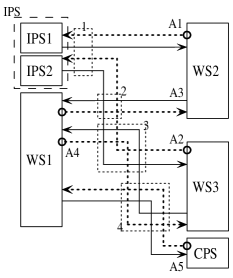
Figure 14: AGV: system configuration

Figure 15: Generators of plant components and specifications

We now apply Algorithm 3 to study a larger example, a system of five automated guided vehicles (AGVs) serving a manufacturing workcell, in the version of [1, Section 4.7], originally adapted from [30].

As displayed in Fig. 14, the workcell consists of two input parts stations IPS1, IPS2 for parts of types 1 and 2, three workstations WS1, WS2, WS3, and one completed parts station CPS. Five independent AGVs – AGV1,…,AGV5 – travel in fixed criss-crossing routes, loading/unloading and transporting parts in the cell. We model the synchronous product of the five AGVs as the plant to be controlled, on which three types of control specifications are imposed: the mutual exclusion (i.e., single occupancy) of shared zones (dashed squares in Fig. 14), the capacity limit of workstations, and the mutual exclusion of the shared loading area of the input stations. The generator models of plant components and specifications are displayed in Fig. 15; here odd numbered events are controllable, and there are 10 such events, $i1,i3$, $i=1,...,5$. For observable events, we will consider different subsets of events below. The reader is referred to [1, Section 4.7] for the detailed interpretation of events.

Under full observation, we obtain by Algorithm 2 the monolithic supervisor of 4406 states and 11338 transitions. Then we select different subsets of controllable events to be unobservable, and apply Algorithm 3 to compute the corresponding supervisors which are relatively observable and controllable. The computational results are displayed in Table I; the supervisors are state minimal, and controllability, observability, and normality are independently verified. All computations and verifications are done by procedures implemented in [29].

The cases in Table I show considerable differences in state size between relatively observable and controllable supervisors and the normal counterparts. In the case $\Sigma_{uo}=\{13\}$, the monolithic supervisor is in fact observable in the standard sense; thus Algorithms 1 and 3 both terminate after 1 iteration, and no transition removing or state unmarking was done. By contrast, the normal supervisor loses 890 states. The contrast in state size is more significant in the case $\Sigma_{uo}=\{21\}$: while the normal supervisor is empty, the relatively observable supervisor loses merely 58 states compared to the full-observation supervisor. The last row of Table I shows a case where only two out of ten controllable events, 11 and 21, are observable. Still, relative observability produces a 579-state supervisor, whereas the normal supervisor is already empty when only events 41 and 51 are unobservable (the third case). Finally, comparing the last two rows of Table I we see that making event 11 (“AGV1 enters zone1”) unobservable substantially reduces the supervisor’s state size, and, indeed, the effect is more substantial than making six other events $\{13,23,33,43,51,53\}$ unobservable. Such a comparison allows us to identify which event(s) may be observationally critical with respect to controlled behavior.

Note from the state sizes of relatively observable supervisors in Table I that no state increase occurs compared to the full-observation supervisor. In addition, the last two columns of Table I suggest that Algorithm 3 with Algorithm 1 embedded terminates reasonably fast.

TABLE I: Test results of Algorithm 3 for different subsets of unobservable events in the AGV system

$\Sigma_{uo}=\Sigma-\Sigma_{o}$	State # of rel. obs. supervisor	State # of normal supervisor	Iteration # of Alg. 3	Iteration # of Alg. 1
{13}	4406	3516	1	1
{21}	4348	0	1	399
{41,51}	3854	0	2	257
{31,43}	4215	1485	1	233
{11,31,41}	163	0	1	28
{13,23,31,33,	579	0	3	462
41,43,51,53}

VI Conclusions

We have identified the new concept of relative observability, and proved that it is stronger than observability, weaker than normality, and preserved under set union. Hence there exists the supremal relatively observable sublanguage of a given language. In addition we have provided an algorithm to effectively compute the supremal sublanguage.

Combined with controllability, relative observability generates generally larger controlled behavior than the normality counterpart. This has been demonstrated with a Guideway example and an AGV example. Empirical results for the AGV example show considerable improvement of controlled behavior using relative observability as compared to normality.

Newly identified, the algebraically well-behaved concept of relative observability may be expected to impact several closely related topics such as coobservability, decentralized supervisory control, stated-based observability, and observability of timed discrete-event systems. In future work we aim to explore these directions.

References

- [1] W. M. Wonham, “Supervisory Control of Discrete-Event Systems,” Systems Control Group, ECE Dept, University of Toronto, updated July 1, 2013. Available online at http://www.control.toronto.edu/DES.
- [2] C. G. Cassandras and S. Lafortune, Introduction to Discrete Event Systems. Springer, 2nd ed, 2007.
- [3] F. Lin and W. M. Wonham, “On observability of discrete-event systems,” Inform. Sci., vol. 44, pp. 173–198, 1988.
- [4] R. Cieslak, C. Desclaux, A. S. Fawaz, and P. Varaiya, “Supervisory control of discrete-event processes with partial observations,” IEEE Trans. Autom. Control, vol. 33, no. 3, pp. 249–260, 1988.
- [5] H. Cho and S. I. Marcus, “On supremal languages of classes of sublanguages that arise in supervisor synthesis problems with partial observation,” Math. of Control, Signals, and Systems, vol. 2, no. 1, pp. 47–69, 1989.
- [6] R. D. Brandt, V. Garg, R. Kumar, F. Lin, S. I. Marcus, and W. M. Wonham, “Formulas for calculating supremal controllable and normal sublanguages,” Systems & Control Letters, vol. 15, no. 2, pp. 111–117, 1990.
- [7] J. Komenda and J. van Schuppen, “Control of discrete-event systems with partial observations using coalgebra and coinduction,” Discrete Event Dynamic Systems, vol. 15, no. 3, pp. 257–315, 2005.
- [8] S. Takai and T. Ushio, “Effective computation of an Lm(G)-closed, controllable, and observable sublanguage arising in supervisory control,” Systems & Control Letters, vol. 49, no. 3, pp. 191–200, 2003.
- [9] H. Cho and S. I. Marcus, “Supremal and maximal sublanguages arising in supervisor synthesis problems with partial observations,” Math. Systems Theory, vol. 22, no. 3, pp. 177–211, 1989.
- [10] J. Fa, X. Yang, and Y. Zheng, “Formulas for a class of controllable and observable sublanguages larger than the supremal controllable and normal sublanguages,” Systems & Control Letters, vol. 20, no. 1, pp. 11–18, 1993.
- [11] M. Heymann and F. Lin, “On-line control of partially observed discrete event systems,” Discrete Event Dynamic Systems, vol. 4, no. 3, pp. 221–236, 1994.
- [12] N. B. Hadj-Alouane, S. Lafortune, and F. Lin, “Centralized and distributed algorithms for on-line synthesis of maximal control policies under partial observation,” Discrete Event Dynamic Systems, vol. 6, no. 4, pp. 379–427, 1996.
- [13] T. Ushio, “On-line control of discrete event systems with a maximally controllable and observable sublanguage,” IEICE Trans. Fundamentals, vol. E82-A, no. 9, pp. 1965–1970, 1999.
- [14] K. Rudie and W. M. Wonham, “Think globally, act locally: decentralized supervisory control,” IEEE Trans. Autom. Control, vol. 37, no. 11, pp. 1692–1708, 1992.
- [15] T. S. Yoo and S. Lafortune, “A general architecture for decentralized supervisory control of discrete-event systems,” Discrete Event Dynamic Systems, vol. 12, no. 3, pp. 335–377, 2002.
- [16] Y. Li and W. M. Wonham, “Controllability and observability in the state-feedback control of discrete-event systems,” in Proc. 27th IEEE Conf. Decision and Control, Austin, TX, 1988, pp. 203–208.
- [17] R. Kumar, V. K. Garg, and S. I. Marcus, “Predicates and predicate transformers for supervisory control of discrete event dynamical systems,” IEEE Trans. Autom. Control, vol. 38, no. 2, pp. 232–247, 1993.
- [18] F. Lin and W. M. Wonham, “Supervisory control of timed discrete-event systems under partial observation,” IEEE Trans. Autom. Control, vol. 40, no. 3, pp. 558–562, 1995.
- [19] S. Takai and T. Ushio, “A new class of supervisors for timed discrete event systems under partial observation,” Discrete Event Dynamic Systems, vol. 16, no. 2, pp. 257–278, 2006.
- [20] H. Marchand, O. Boivineau, and S. Lafortune, “Optimal control of discrete event systems under partial observation,” in Proc. 40th IEEE Conf. Decision and Control, Orlando, FL, 2001, pp. 2335–2340.
- [21] F. Lin and W. M. Wonham, “Decentralized control and coordination of discrete-event systems with partial observation,” IEEE Trans. Autom. Control, vol. 35, no. 12, pp. 1330–1337, 1990.
- [22] R. Su, J. H. van Schuppen, and J. E. Rooda, “Aggregative synthesis of distributed supervisors based on automaton abstraction,” IEEE Trans. Autom. Control, vol. 55, no. 7, pp. 1627–1640, 2010.
- [23] J. Komenda, T. Masopust, and J. van Schuppen, “Synthesis of controllable and normal sublanguages for discrete-event systems using a coordinator,” Systems & Control Letters, vol. 55, no. 7, pp. 1627–1640, 2011.
- [24] W. M. Wonham and P. J. Ramadge, “On the supremal controllable sublanguage of a given language,” SIAM J. of Control and Optimization, vol. 25, no. 3, pp. 637–659, 1987.
- [25] B. A. Davey and H. A. Priestley, Introduction to Lattices and Order. Cambridge University Press, 1990.
- [26] J. N. Tsitsiklis, “On the control of discrete-event dynamical systems,” Math. of Control, Signals, and Systems, vol. 2, no. 2, pp. 95–107, 1989.
- [27] L. Feng and W. M. Wonham, “Supervisory control architecture for discrete-event systems,” IEEE Trans. Autom. Control, vol. 53, no. 6, pp. 1449–1461, 2008.
- [28] ——, “On the computation of natural observers in discrete-event systems,” Discrete Event Dyna. Syst., vol. 20, no. 1, pp. 63–102, 2010.
- [29] W. M. Wonham, “Design software: XPTCT,” Systems Control Group, ECE Dept, University of Toronto, updated July 1, 2013. Available online at http://www.control.toronto.edu/DES.
- [30] L. E. Holloway and B. H. Krogh, “Synthesis of feedback logic control for a class of controlled petri nets,” IEEE Trans. Autom. Control, vol. 35, no. 5, pp. 514–523, 1990.