[1306.2419] 1 Plots of the radius function 𝑏, coverage probability and scaled expected volume (as functions of 𝛾=‖𝜽‖) for both the new RCS and the RCS of Casella and Hwang (1983, Section 4), for 1-𝛼=0.95 and 𝑝=3.

A new recentered confidence sphere for the multivariate normal mean

Waruni Abeysekera and Paul Kabaila^∗

La Trobe University

^∗ Author to whom correspondence should be addressed.

Department of Mathematics and Statistics, La Trobe University, Victoria 3086, Australia.

e-mail: P.Kabaila@latrobe.edu.au

Facsimile: 3 9479 2466

Telephone: 3 9479 2594

Abstract

We describe a new recentered confidence sphere for the mean, $\boldsymbol{\theta}$ , of a multivariate normal distribution. This sphere is centred on the positive-part James-Stein estimator, with radius that is a piecewise cubic Hermite interpolating polynomial function of the norm of the data vector. This radius function is determined by numerically minimizing the scaled expected volume, at $\boldsymbol{\theta}=\boldsymbol{0}$ , of this confidence sphere, subject to the coverage constraint. We use the computationally-convenient formula, derived by Casella and Hwang, 1983, JASA, for the coverage probability of a recentered confidence sphere. Casella and Hwang, op. cit., describe a recentered confidence sphere that is also centred on the positive-part James-Stein estimator, but with radius function determined by empirical Bayes considerations. Our new recentered confidence sphere compares favourably with this confidence sphere, in terms of both the minimum coverage probability and the scaled expected volume at $\boldsymbol{\theta}=\boldsymbol{0}$ .

Keywords and phrases: confidence set, multivariate normal mean, recentered confidence sphere.

1. Introduction

Suppose that $\boldsymbol{X}=\left(X_{1},...,X_{p}\right)\sim N\left(\boldsymbol{\theta},\sigma^{2}\boldsymbol{\textbf{I}_{p}}\right)$ where $\boldsymbol{\theta}=\left(\theta_{1},...,\theta_{p}\right)$ and $\boldsymbol{\textbf{I}_{p}}$ denotes the $p\times p$ identity matrix. We consider the problem of finding a confidence set for $\boldsymbol{\theta}$ , based on $\boldsymbol{X}$ , with prescribed confidence coefficient $1-\alpha$ that satisfies the following two conditions. The first condition is that this confidence set has volume that never exceeds the volume of the standard $1-\alpha$ confidence sphere centred at $\boldsymbol{X}$ . The second condition is that this confidence set has an expected volume that is small by comparison with that of the standard $1-\alpha$ confidence sphere, when $\boldsymbol{\theta}=\boldsymbol{0}$ . Casella and Hwang (1987) argue cogently that the confidence set for $\boldsymbol{\theta}$ should be tailored to the uncertain prior information available about $\boldsymbol{\theta}$ . We consider confidence sets that are tailored to the uncertain prior information that $\boldsymbol{\theta}=\boldsymbol{0}$ . The second condition is motivated by a desire to utilize this uncertain prior information. This is a very difficult problem to solve and, in common with much of the existing literature on it, we assume that $\sigma^{2}$ is known. Without loss of generality, we assume that $\sigma^{2}=1$ . The standard $1-\alpha$ confidence set for $\boldsymbol{\theta}$ is $I=\{\boldsymbol{\theta}:\,\|\boldsymbol{\theta}-\boldsymbol{X}\|\leq d\}$ , where the positive number $d$ satisfies $P\big{(}Q\leq d^{2}\big{)}=1-\alpha$ for $Q\sim\chi_{p}^{2}$ .

The early work of Stein (1962), Brown (1966), Joshi (1967) and Hwang and Casella (1982) that relates to this problem is reviewed by Casella and Hwang (2012). Confidence sets for $\boldsymbol{\theta}$ , of various shapes, that solve this problem have been proposed by Faith (1976), Berger (1980), Casella and Hwang (1983, 1987), Shinozaki (1989), Tseng and Brown (1997), Samworth (2005) and Efron (2006). These confidence sets are reviewed and compared by Efron (2006) and Casella and Hwang (2012).

To provide specific proposals for recentered confidence spheres, Casella and Hwang (1983, 1987) and Samworth (2005) center their confidence spheres at the positive-part James-Stein estimator. The radii of these confidence spheres are functions of $||\boldsymbol{X}||$ that are determined by empirical Bayes considerations (Casella and Hwang, 1983), Taylor series or the bootstrap (Samworth, 2005). These papers compare confidence sets for $\boldsymbol{\theta}$ using the coverage probability and the scaled volume (or its $p$ ’th root).

In the present paper, we also consider a confidence sphere for $\boldsymbol{\theta}$ that is centered at the positive-part James-Stein estimator. However, we have chosen the radius of this confidence sphere to be a piecewise cubic Hermite interpolating polynomial function of $||\boldsymbol{X}||$ . This radius function is required to be both nondecreasing and bounded above by $d$ . This function is determined by numerically minimizing the scaled expected volume of this confidence sphere at $\boldsymbol{\theta}=\boldsymbol{0}$ , subject to the constraint that the coverage probability never falls below $1-\alpha$ . Here, the scaled expected volume is defined to be the ratio (expected volume of the recentered confidence sphere) / (volume of $I$ ). This numerical constrained minimization is made feasible by the fact that both the coverage probability and the scaled expected volume of a recentered confidence sphere are functions of $\gamma=||\boldsymbol{\theta}||$ , for a given radius function. We use the computationally-convenient formula, derived by Casella and Hwang (1983), for the coverage probability of a recentered confidence sphere for $p$ odd.

The two main contributions of the present paper are the following:

(1)

We shift the focus from scaled volume (or its $p$ ’th root) to scaled expected volume. A goal of seeking to minimize (in some sense) the volume of the recentered confidence sphere for the most probable values of $\boldsymbol{X}$ when $\boldsymbol{\theta}=\boldsymbol{0}$ , subject to the coverage constraint, is problematic (Casella and Hwang, 1986). By contrast, as we show in the present paper, minimization of the scaled expected volume of the recentered confidence sphere (RCS) at $\boldsymbol{\theta}=\boldsymbol{0}$ , subject to the coverage constraint, leads to a RCS with excellent performance.
(2)

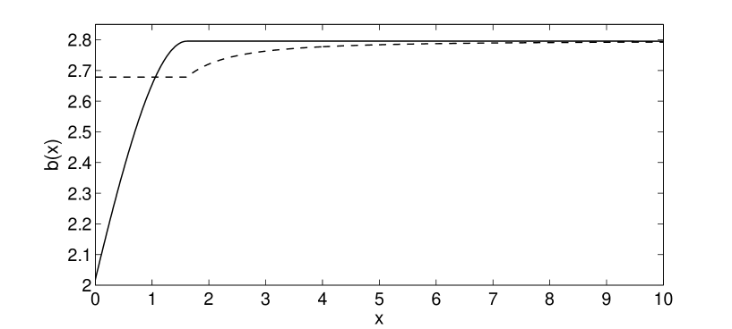
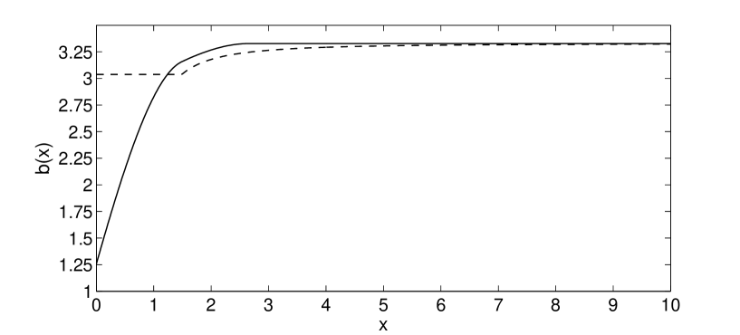
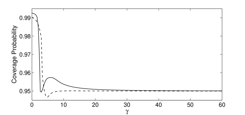
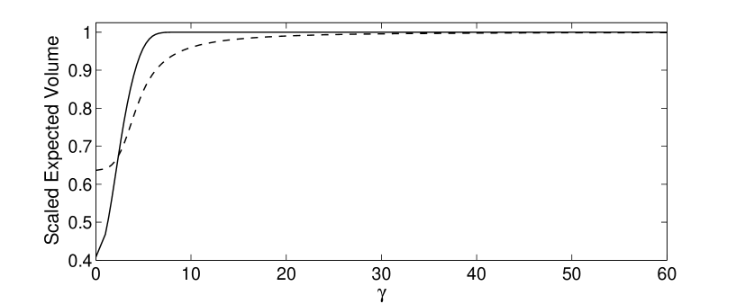
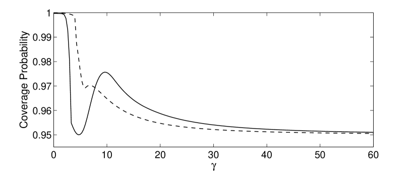
Our new RCS compares favourably with the RCS described in Section 4 of Casella and Hwang (1983), in terms of both the minimum coverage probability and the scaled expected volume at $\boldsymbol{\theta}=\boldsymbol{0}$ . This is shown in Figure 1, 2 and 3, which are for $1-\alpha=0.95$ and $p=3,5$ and $15$ , respectively. The bottom panel and middle panel in each of these figures compare the coverage probability and scaled expected volume, respectively, of the new RCS and the RCS of Casella and Hwang (1983, Section 4).

2. Performance of the new RCS by comparison with the RCS of Casella and Hwang (1983, Section 4)

Both the RCS of Casella and Hwang (1983, Section 4) and the new RCS are centered on the positive-part James-Stein estimator. These RCS’s take the form $J(b)=\big{\{}\boldsymbol{\theta}:\|a^{+}(T)\boldsymbol{X}-\boldsymbol{\theta}\|\leq b(T)\big{\}}$ , where $T=||\boldsymbol{X}||/\sqrt{p}$ ,

a^{+}(x)=\text{max}\left\{0,1-\left(1-\frac{2}{p}\right)\frac{1}{x^{2}}\right\},

and $b:[0,\infty)\rightarrow(0,\infty)$ is required to be a nondecreasing function that is bounded above by $d$ . We call $b$ the radius function. We use a slightly different notation for a RCS from that used by Casella and Hwang (1983), who express a RCS in terms of $||\boldsymbol{X}||$ .

We define the scaled expected volume of $J(b)$ to be the ratio

\frac{E_{\boldsymbol{\theta}}(\text{volume of }J(b))}{\text{volume of }I}=E_{\boldsymbol{\theta}}\left(\left(\frac{b(T)}{d}\right)^{p}\right),

(1)

since the volume of a sphere in $\mathbb{R}^{p}$ with radius $r$ is $2\,r^{p}\,\pi^{p/2}/\big{(}p\,\Gamma(p/2)\big{)}$ . As proved in the Appendix, this is a function of $\gamma=||\boldsymbol{\theta}||$ , for given function $b$ . It can also be shown that the coverage probability of $J(b)$ is a function of $\gamma$ , for given function $b$ .

For computational feasibility, we specify the following parametric form for the radius function $b$ . Suppose $b(x)=d$ for all $x\geq k$ , where $k$ is a (sufficiently large) specified positive number. Suppose that $x_{1},\dots,x_{q}$ satisfy $0=x_{1}<x_{2}<\dots<x_{q}=k$ . The function $b$ is fully specified by the vector $b(x_{1}),\dots,b(x_{q})$ as follows. The value of $b(x)$ for any given $x\in[0,k]$ is found by piecewise cubic Hermite polynomial interpolation for these given function values. We call $x_{1},\dots,x_{q}$ the knots.

For judiciously-chosen values of the knots, we compute the function $b$ , which takes this parametric form, is nondecreasing and is bounded above by $d$ , such that (a) the scaled expected volume evaluated at $\boldsymbol{\theta}=\boldsymbol{0}$ (i.e. at $\gamma=0$ ) is minimized and (b) the coverage probability of $J(b)$ never falls below $1-\alpha$ .

This coverage constraint is implemented in the computations as follows. For any reasonable choice of the function $b$ , the coverage probability of $J(b)$ converges to $1-\alpha$ as $\gamma\rightarrow\infty$ . The constraints implemented in the computations are that the coverage probability of $J(b)$ is greater than or equal to $1-\alpha$ for every $\gamma$ in a judiciously-chosen finite set of values. That a given finite set of values of $\gamma$ is adequate to the task is judged by checking numerically, at the completion of computations, that the coverage probability constraint is satisfied for all $\gamma\geq 0$ .

This type of computation has been carried out in other related problems by Farchione and Kabaila (2008, 2012) and Kabaila and Giri (2009ab, 2013ab). The main lesson from these related computations is that the coverage probability needs to be computed with great accuracy. Fortunately, in the context of the present paper, the coverage probability of $J(b)$ can be computed with great accuracy for $p$ odd, using the formula derived by Casella and Hwang (1983). Note that there is a typographical error in this formula as stated on page 691 of Casella and Hwang (1983). The $(n+1)!$ on the second line of (3.10) should be replaced by $(n+i)!$ . To help ensure accurate computation of the coverage probability, progressive numerical quadrature, using Simpson’s rule and a doubling of equal-length segments at each stage of the progression is used. The main stopping criterion is that $|Q_{2s}-Q_{s}|/Q_{2s}\leq 10^{-8}$ , where $Q_{s}$ denotes the computed quadrature using $s$ segments. All of the computations presented in the present paper were performed using programs written in MATLAB using the Statistics and Optimization toolboxes.

We now compare the coverage probability and scaled expected volume properties of the new RCS and the RCS of Casella and Hwang (1983, Section 4), which uses the following radius function

b(x)=\begin{cases}\sqrt{(1-(p-2)/d^{2})(d^{2}-p\,\log(1-(p-2)/d^{2}))}&\text{for }x\in[0,d/\sqrt{p}]\\ \sqrt{(1-(p-2)/(p\,x^{2}))(d^{2}-p\,\log(1-(p-2)/(p\,x^{2})))}&\text{for }x>d/\sqrt{p}.\end{cases}

This radius function was determined by empirical Bayes considerations.

For $1-\alpha=0.95$ , the new RCS was computed for each $p\in\{3,5,7,9,11,13,15,17,19\}$ . We restrict to odd values of $p$ in order to use the computationally-convenient formula for the coverage probability derived by Casella and Hwang (1983) for $p$ odd. We have chosen $k=10$ . The positions of the knots of $b$ have been chosen to depend on $p$ as follows. The first two knots are at 0 and $d/\sqrt{p}$ . The next two knots are at $(d/\sqrt{p})+c$ and $(d/\sqrt{p})+2c$ , where $c=((k/2)-(d/\sqrt{p}))/3$ . The remaining knots are at $k/2$ , $3k/4$ and $k$ . The coverage constraint was implemented in the computations by requiring that the coverage probability of $J(b)$ is greater than or equal to $1-\alpha$ for all $\gamma\in\{0,1,2,\dots,64,65\}$ . This was shown to be adequate to the task by checking numerically, at the completion of the computation of the new RCS, that the coverage probability constraint is satisfied for all $\gamma\geq 0$ .

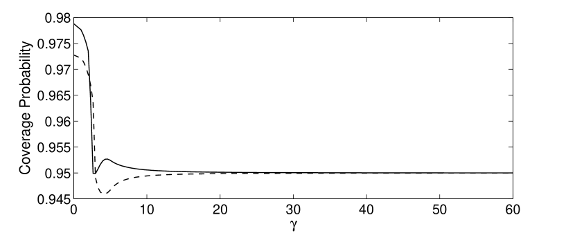
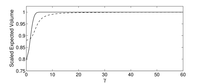
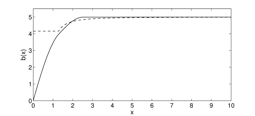
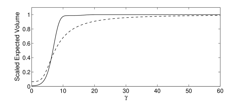
Figures 1, 2 and 3 compare the radius functions $b$ , coverage probabilities and scaled expected volumes of the new RCS and the RCS of Casella and Hwang (1983, Section 4) for $1-\alpha=0.95$ and $p=3,5$ and $15$ , respectively. The top panel of each of these figures compares the radius functions $b$ . The difference between the radius functions of these RCS’s is substantial for $p=3$ and increases as $p$ increases. The middle panel compares the coverage probabilities of these RCS’s as functions of $\gamma=||\boldsymbol{\theta}||$ . The bottom panel compares the scaled expected volumes of these RCS’s as functions of $\gamma$ .

Figure 1 shows that, for $p=3$ , the coverage probability (CP) of the new RCS is no less than $0.95$ for all $\gamma$ values, while the CP of the RCS of Casella and Hwang (1983, Section 4) is slightly below $0.95$ at some $\gamma$ values. This figure also shows that, for $p=3$ , the scaled expected volume (SEV) at $\boldsymbol{\theta}=\boldsymbol{0}$ of the new RCS is substantially less than the SEV at $\boldsymbol{\theta}=\boldsymbol{0}$ of the RCS of Casella and Hwang (1983, Section 4). Figure 2 tells a similar story for $p=5$ . Figure 3, which is for the case $p=15$ , shows that the new RCS performs substantially better than the RCS of Casella and Hwang (1983, Section 4), in terms of SEV at $\boldsymbol{\theta}=\boldsymbol{0}$ . However, for this value of $p$ , both RCS’s maintain a CP that is greater than or equal to $0.95$ . The computations of the CP and SEV of these RCS’s were checked using Monte Carlo simulations.

Table 1 presents a comparison of the minimum CP’s and the SEV’s at $\boldsymbol{\theta}=\boldsymbol{0}$ of these RCS’s for $p\in\{3,5,7,9,11,13,15,17,19\}$ . According to this table, the new RCS always achieves a CP greater than or equal to $0.95$ , while the RCS of Casella and Hwang (1983, Section 4) does not achieve this for $p=3$ and $p=5$ . Also, for every value of $p$ considered, the new RCS achieves a substantially lower SEV at $\boldsymbol{\theta}=\boldsymbol{0}$ than the RCS of Casella and Hwang (1983, Section 4). In summary, our new RCS compares favourably with that of Casella and Hwang (1983, Section 4), in terms of both the minimum CP and the SEV at $\boldsymbol{\theta}=\boldsymbol{0}$ .

Refer to caption — Figure 1: Plots of the radius function $b$ , coverage probability and scaled expected volume (as functions of $\gamma=||\boldsymbol{\theta}||$ ) for both the new RCS and the RCS of Casella and Hwang (1983, Section 4), for $1-\alpha=0.95$ and $p=3$ .

$p$	RCS of Casella & Hwang (1983, Section 4)		new RCS
	minimum CP	SEV at $\boldsymbol{\theta}=\boldsymbol{0}$	minimum CP	SEV at $\boldsymbol{\theta}=\boldsymbol{0}$
3	0.94594	0.88054	0.95	0.79435
5	0.94662	0.63637	0.95	0.40805
7	0.95	0.43315	0.95	0.19833
9	0.95	0.28243	0.95	0.09245
11	0.95	0.17794	0.95	0.04127
13	0.95	0.10889	0.95	0.01831
15	0.95	0.06498	0.95	0.00804
17	0.95	0.03791	0.95	0.00357
19	0.95	0.02169	0.95	0.00272

Table 1: Comparison of the new RCS and the RCS of Casella and Hwang (1983, Section 4), with respect to the minimum coverage probability and the scaled expected volume at

\boldsymbol{\theta}=\boldsymbol{0}

, for

1-\alpha=0.95

and

p\in\{3,5,7,9,11,13,15,17,19\}

Remark 2.1: We have chosen the radius function $b$ to be a piecewise cubic Hermite interpolating polynomial in the interval $[0,k]$ . Other choices of parametric forms for this function are also possible. For example, one could choose this function to be a cubic spline in this interval.

Remark 2.2: Casella and Hwang (1983, Section 3) argue that it is desirable that the set $S_{\theta}$ , described in their Theorem 3.1, is an interval. During the computation of the new RCS, it was found that at every stage (including the final stage) this set was an interval.

Appendix: Computationally-convenient formula for the scaled expected volume

The following theorem provide a computationally convenient-formula for the scaled expected volume of the recentered confidence sphere $J(b)$ .

Theorem 1.

For given function $b$ , the scaled expected volume of $J(b)$ is a function of $\gamma=||\boldsymbol{\theta}||$ .

(a)

Let $f\big{(}y;p,\gamma^{2}\big{)}$ denote the noncentral $\chi^{2}$ pdf with $p$ degrees of freedom and noncentrality parameter $\gamma^{2}$ , evaluated at $y$ . The scaled expected volume of $J(b)$ is

\int_{0}^{\infty}\left(\frac{b\big{(}\sqrt{y/p}\big{)}}{d}\right)^{p}f\big{(}y;p,\gamma^{2}\big{)}\,dy.

(2)

(b)

Suppose that $b(x)=d$ for all $x\geq k$ , where $k$ is a specified positive number. The scaled expected volume of $J(b)$ is

\int_{0}^{pk^{2}}\left(\frac{b\big{(}\sqrt{y/p}\big{)}}{d}\right)^{p}f\big{(}y;p,\gamma^{2}\big{)}\,dy+1-F\big{(}pk^{2};p,\gamma^{2}\big{)},

(3)

where $F\big{(}y;p,\gamma^{2}\big{)}$ denotes the noncentral $\chi^{2}$ cdf with $p$ degrees of freedom and noncentrality parameter $\gamma^{2}$ , evaluated at $y$ .

Proof.

Note that $Y=||\boldsymbol{X}||^{2}=X_{1}^{2}+\dots+X_{p}^{2}$ has a noncentral $\chi^{2}$ distribution with $p$ degrees of freedom and noncentrality parameter $\gamma^{2}$ . It follows from (1) that the scaled expected volume of $J(b)$ is (2). Clearly, (2) is a function of $\gamma$ , for given function $b$ .

Suppose that $b(x)=d$ for all $x\geq k$ , where $k$ is a specified positive number. Obviously, (3) follows immediately from (2).

∎

Suppose that the radius function $b$ is a piecewise cubic Hermite interpolating polynomial in the interval $[0,k]$ , with knots at $x_{1},\dots,x_{q}$ ( $0=x_{1}<x_{2}<\dots<x_{q}=k$ ), that takes the value $d$ for all $x\geq k$ . This function is very smooth between between successive knots (it is a cubic between these knots). However, it may not possess a second derivative at each of the knots. For this reason, we use this theorem to compute the scaled expected volume of $J(b)$ using the formula

\sum_{i=1}^{q-1}\int_{px_{i}^{2}}^{px_{i+1}^{2}}s(y;b,\gamma)\,dy+1-F\big{(}pk^{2};p,\gamma^{2}\big{)},

where each integral is computed separately by numerical quadrature.

References

BERGER, J. (1980). A robust generalized Bayes estimator and confidence region for a multivariate normal mean. Annals of Statistics, 8, 716–761.

BROWN, L.D. (1966). On the admissibility of invariant estimators of one or more location parameters. Annals of Mathematical Statistics, 37, 1087–1136.

CASELLA, G. and HWANG, J.T. (1983). Empirical Bayes confidence sets for the mean of a multivariate normal distribution. Journal of the American Statistical Association, 78, 688–698.

CASELLA, G. and HWANG, J.T. (1986). Confidence sets and the Stein effect. Communications in Statistics – Theory and Methods, 15, 2043–2063.

CASELLA, G. and HWANG, J.T. (1987). Employing vague prior information in the construction of confidence sets. Journal of Multivariate Analysis, 21, 79–104.

CASELLA, G. and HWANG, J.T. (2012). Shrinkage confidence procedures. Statistical Science, 27, 51–60.

EFRON, B. (2006). Minimum volume confidence regions for a multivariate normal mean vector. Journal of the Royal Statistical Society, Series B, 68, 655–670.

FARCHIONE, D. and KABAILA, P. (2008). Confidence intervals for the normal mean utilizing prior information. Statistics & Probability Letters, 78, 1094–1100.

FARCHIONE, D. and KABAILA, P. (2012). Confidence intervals in regression centred on the SCAD estimator. Statistics & Probability Letters, 82, 1953–1960.

FAITH, R.E. (1976). Minimax Bayes point and set estimators of a multivariate normal mean. Unpublished PhD thesis, Department of Statistics, University of Michigan.

HWANG, J.T. and CASELLA, G.(1982). Minimax confidence sets for the mean of a multivariate normal distribution. Annals of Statistics, 10, 868–881.

JOSHI, V.M. (1967) Inadmissibility of the usual confidence sets for the mean of multivariate normal population. Annals of Mathematical Statistics, 38, 1868–1875.

KABAILA, P. and GIRI, K. (2009a). Confidence intervals in regression utilizing uncertain prior information. Journal of Statistical Planning and Inference, 139, 3419–3429.

KABAILA, P. and GIRI, K. (2009b). Large-sample confidence intervals in a two-period crossover, utilizing uncertain prior information. Statistics & Probability Letters, 79, 652–658.

KABAILA, P. and GIRI, K. (2013a). Simultaneous confidence intervals for the population cell means, for two-by-two factorial data, that utilize uncertain prior information. To appear in Communications in Statistics: Theory and Methods.

KABAILA, P. and GIRI, K. (2013b). Further properties of frequentist confidence intervals in regression that utilize uncertain prior information. To appear in Australian & New Zealand Journal of Statistics.

SAMWORTH, R. (2005). Small confidence sets for the mean of a spherically symmetric distribution. Journal of the Royal Statistical Society, Series B, 67, 343–361.

SHINOZAKI, N. (1989). Improved confidence sets for the mean of a multivariate normal distribution. Annals of the Institute of Mathematical Statistics, 41, 331–346.

STEIN, C. (1962). Confidence sets for the mean of a multivariate normal distribution. Journal of the Royal Statistical Society, Series B, 9, 1135–1151.

TSENG, Y.L. and BROWN, L.D. (1997). Good exact confidence sets for a multivariate normal mean. Annals of Statistics, 5, 2228–2258.