Information amplification via postselection: A parameter estimation perspective

Abstract

It is known that weak measurement can significantly amplify the mean of measurement results, sometimes out of the range limited in usual quantum measurement. This fact, as actively demonstrated recently in both theory and experiment, implies the possibility to estimate a very small parameter using the weak measurement technique. But does the weak measurement really bring about the increase of ginformation h for parameter estimation? This paper clarifies that, in a general situation, the answer is NO; more precisely, the weak measurement cannot further decrease the lower bound of the estimation error, i.e. the so-called Cram Ler-Rao bound, which is proportional to the inverse of the quantum Fisher information.

I Signal amplification and parameter estimation

The importance of quantum metrology is self-evident in a wide area of applications such as the atomic clock and gravitational wave detection Giovannetti . The most simple form of this problem is to estimate an unknown small parameter $\theta$ contained in the unitary evolution $\hat{U}=\exp(-i\theta\hat{H})$, where the Hamiltonian $\hat{H}$ is assumed to be known.

Among various approaches to this problem, a specifically attractive one is the method based on weak measurement AAVPRL1988 , in the situation where $\hat{H}$ is an interaction Hamiltonian and we want to estimate the interaction strength $\theta$. The method is briefly described as follows; For a system ${\cal H}$ and a probe ${\cal K}$, an interaction Hamiltonian $\hat{H}=\hat{A}^{\cal H}\otimes\hat{p}^{\cal K}$ with $\hat{p}^{\cal K}$ the probe momentum operator is given to us. (In what follows we will omit the subscript ${\cal H}$ or ${\cal K}$ when obvious.) Also, we are allowed to freely set a system’s initial state $|{i}\rangle_{\cal H}$ and a final state $|{f}\rangle_{\cal H}$, which are respectively called pre and post selection. Then, for a small $\theta$, the probe position operator $\hat{x}^{\mathcal{K}}$ satisfying $[\hat{x},\hat{p}]=i$ experiences a shift proportional to the weak value $\langle{\hat{A}}\rangle_{w}:=\langle{f|\hat{A}|i}\rangle/\langle{f|i}\rangle$; in fact, the mean value is given by (see CWV )

$$\langle{\hat{x}^{\mathcal{K}}}\rangle\propto\theta\cdot\mathrm{Re}\langle{\hat{A}}\rangle_{w}.$$ (1)

This implies that, by choosing a nearly orthogonal pair of $|{i}\rangle$ and $|{f}\rangle$, we obtain a largely amplified signal $\langle{\hat{x}^{\mathcal{K}}}\rangle$, which would give us a chance to estimate $\theta$ highly accurately. This signal’s amplification technique was originally developed by Hosten et al. in an application to detect the spin hall effect of light Hosten . Also Dixson et al. have demonstrated the detection of a slight tilt of a mirror in a Sagnac interferometer Dixson . Furthermore, in some recent works WuLi ; KT ; Nakamura ; Nishizawa ; Susa2012 ; LeeTsutsui it was clarified that the amplification is still possible to a certain extent even when $\theta$ is not small.

The above-described method, however, lacks a statistical viewpoint for analyzing how accurate we can estimate the parameter $\theta$. In other words, rather than the mean, we should evaluate the estimation error, based on quantum statistics Helstrom ; Holevo ; Braunstein ; Holevo2001 ; Hayashi . Especially in our case we invoke the theory of a one-parameter estimation described as follows; When $n$ independent copies of a state $\hat{S}_{\theta}$ with single parameter $\theta$ are given to us, any estimator (an observable to be measured) $\hat{T}$ is limited in estimation performance by the quantum Cramér-Rao inequality

$$\langle{(\hat{T}-\theta\hat{I})^{2}}\rangle_{\hat{S}_{\theta}}={\rm Tr}\big{[}\hat{S}_{\theta}(\hat{T}-\theta\hat{I})^{2}\big{]}\geq\frac{1}{nI(\hat{S}_{\theta})}.$$ (2)

Here, $I(\hat{S}_{\theta})$ is the SLD quantum Fisher information:

$$I(\hat{S}_{\theta}):=\langle\hat{L}_{\theta}^{2}\rangle_{\hat{S}_{\theta}}={\rm Tr}\big{[}\hat{L}_{\theta}^{2}\hat{S}_{\theta}\big{]},$$ (3)

where $\hat{L}_{\theta}$ is a Hermitian operator called the symmetric logarithmic derivative (SLD) satisfying the following linear algebraic equation:

$$\partial_{\theta}\hat{S}_{\theta}=\frac{1}{2}\left(\hat{S}_{\theta}\hat{L}_{\theta}+\hat{L}_{\theta}\hat{S}_{\theta}\right).$$ (4)

In this paper, we simply call Eq. (3) the Fisher information. Equation (2) means that a state with larger Fisher information allows us to estimate the parameter $\theta$ with better accuracy. Actually, despite that the Cramér-Rao bound $1/nI(\hat{S}_{\theta})$ generally depends on the unknown parameter $\theta$, there have been developed some estimation techniques to attain the equality in Eq. (2) Nagaoka ; Fujiwara_MLE .

From the above discussion, we should turn our attention from the mean to the Fisher information, for evaluating possible advantages of the weak measurement technique in signal amplification in the sense of parameter estimation. That is, our question is the following; Does the weak measurement amplify the information for parameter estimation, in the sense of Fisher information multiplied by the number of copies of the state (i.e. the inverse of the Cramér-Rao bound)? Actually this problem has been studied by Knee et al. in Knee in a specific example and they found that the Cramér-Rao bound cannot be decreased by weak measurement (and more broadly by postselection as mentioned later). This fact leads us to have a negative impression for the use of weak measurement technique in parameter estimation problems. The main contribution of this paper is to clarify that the answer to the above question is NO; that is, we prove that, in a general situation, the weak measurement cannot decrease the Cramér-Rao bound.

Before closing this section, we make two remarks. First, in the literature there are several works addressing the weak measurement in the framework of parameter estimation, particularly with classical Fisher information Hofmann ; Shikano ; Strubi ; Viza . Second, as motivated by the previous results WuLi ; KT ; Nakamura ; Nishizawa ; Susa2012 ; LeeTsutsui , we will work on the subject without assuming that $\theta$ is small. In this sense, the scheme is not anymore what is based on weak measurement, rather at the heart of the scheme is the postselection; hence the above question is a bit modified. Note that this problem setting also discerns our work and Knee from Hofmann ; Shikano ; Strubi ; Viza .

II Quantum Fisher information of the postselected state

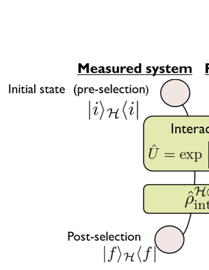
Figure 1: Procedure of the postselection.

We study the composition of a system ${\cal H}$ and a probe ${\cal K}$ with initial state $|{i}\rangle_{\cal H}\langle{i}|\otimes\hat{\rho}_{\mathrm{i}}^{\mathcal{K}}$. This state is subjected to the interaction $\hat{U}=\exp(-i\theta\hat{H})$, which yields

$$\hat{\rho}_{\mathrm{int}}^{\mathcal{H}\otimes\mathcal{K}}=\hat{U}(|{i}\rangle_{\mathcal{H}}\langle{i}|\otimes\hat{\rho}_{\rm i}^{\mathcal{K}})\hat{U}^{\dagger}.$$ (5)

Again, $\theta$ is a single unknown parameter. We then consider a specific state with its system component projected onto a fixed state $|{f}\rangle_{\cal H}$, i.e., the following postselected (ps) state (see Fig. 1):

$$\hat{\rho}^{\mathcal{K}}_{\mathrm{ps}}=\frac{{\rm Tr}_{\mathcal{H}}\big{[}(|{f}\rangle_{\mathcal{H}}\langle{f}|\otimes\hat{I}^{\mathcal{K}})\hat{\rho}_{\mathrm{int}}^{\mathcal{H}\otimes\mathcal{K}}]}{\Pr(f)}=\frac{\hat{B}\hat{\rho}_{\mathrm{i}}^{\mathcal{K}}\hat{B}^{\dagger}}{{\rm Tr}\big{(}\hat{B}\hat{\rho}_{\mathrm{i}}^{\mathcal{K}}\hat{B}^{\dagger}\big{)}},$$ (6)

where $\hat{B}=\mbox{}_{\cal H}\langle{f}|\hat{U}|{i}\rangle_{\mathcal{H}}$ and $\Pr(f)$ is the success probability of the postselection:

$${\rm Pr}(f)={\rm Tr}\big{[}(|{f}\rangle_{\mathcal{H}}\langle{f}|\otimes\hat{I}^{\mathcal{K}})\hat{\rho}_{\rm int}^{\mathcal{H}\otimes\mathcal{K}}\big{]} ={\rm Tr}\big{(}\hat{B}\hat{\rho}_{\mathrm{i}}^{\mathcal{K}}\hat{B}^{\dagger}\big{)}.$$ (7)

What we are concerned with is, under the assumption that both ${\cal H}$ and ${\cal K}$ are accessible as in the case of Hosten ; Dixson , if the postselected state (6) would contain more valuable information than the whole state without conditioning, (5). Hence here we can formulate our first problem; is the Fisher information of the state (6) bigger than that of the state (5)? In general, it is not straightforward to calculate the Fisher information, but in the case of pure states it is uniquely and explicitly obtained. That is, for a pure state $\hat{S}_{\theta}=|{\chi_{\theta}}\rangle\langle{\chi_{\theta}}|$, the Fisher information is given by

$$I(\hat{S}_{\theta})=\langle\hat{L}^{2}\rangle_{\hat{S}_{\theta}}=4\left(\langle{\partial_{\theta}\chi_{\theta}|\partial_{\theta}\chi_{\theta}}\rangle-\bigr{|}\langle{\partial_{\theta}\chi_{\theta}|\chi_{\theta}}\rangle\bigr{|}^{2}\right),$$

where $|{\partial_{\theta}\chi_{\theta}}\rangle=\partial|{\chi_{\theta}}\rangle/\partial\theta$. To use this formula, let us assume $\rho_{\rm i}^{\cal K}=|{\psi}\rangle_{\cal K}\langle{\psi}|$. Then, the Fisher information of the state (5) is obtained as

$$I(\hat{\rho}^{\mathcal{H}\otimes\mathcal{K}}_{\mathrm{int}}) =4\left[\langle{i,\psi}|\hat{H}^{2}|{i,\psi}\rangle-\langle{i,\psi}|\hat{H}|{i,\psi}\rangle^{2}\right]$$

$$=4\bigl{(}\langle{\hat{H}^{2}}\rangle-\langle{\hat{H}}\rangle^{2}\bigr{)},$$ (8)

while that of the postselected state (6) is given by

$$I(\hat{\rho}^{\mathcal{K}}_{\mathrm{ps}})=\frac{4\langle\psi|\partial_{\theta}\hat{B}^{\dagger}\partial_{\theta}\hat{B}|\psi\rangle}{\Pr(f)}-\frac{4|\langle\psi|\partial_{\theta}\hat{B}^{\dagger}\hat{B}|\psi\rangle|^{2}}{\Pr(f)^{2}}.$$ (9)

Here the success probability is $\Pr(f)=\langle{\psi}|\hat{B}^{\dagger}\hat{B}|{\psi}\rangle$. Equation (9) shows that $I(\hat{\rho}^{\mathcal{K}}_{\mathrm{ps}})$ takes a large number, or equivalently the postselected state becomes more valuable, if $\Pr(f)$ is taken to be small by the postselection. In particular, when $\hat{H}=\hat{A}\otimes\hat{p}$, we find that

$$\lim_{\theta\rightarrow 0}I(\hat{\rho}^{\mathcal{K}}_{\mathrm{ps}})=\big{|}\langle{\hat{A}}\rangle_{w}\big{|}^{2}\langle{\psi}|(\hat{p}-\langle{\hat{p}}\rangle)^{2}|{\psi}\rangle.$$ (10)

Hence, in the weak interaction limit $\theta\rightarrow 0$, increasing the weak value $|\langle{\hat{A}}\rangle_{w}|$ via the postselection directly means increase of the Fisher information. This fact leads us to expect that the signal amplification technique based on the weak measurement Hosten ; Dixson ; WuLi ; KT ; Nakamura ; Nishizawa ; Susa2012 ; LeeTsutsui would be statistically consistent.

III Sensitivity amplification via postselection

In this section, we compare the two Fisher informations presented above in a specific example. Note that, as seen in Eq. (2), the Fisher information itself does not provide the lower bound of the estimation error in a repeated experiment; we will discuss this in the next section. Here the Fisher information is identified with the “distinguishability” of states Helstrom ; Holevo ; Braunstein ; Holevo2001 ; Hayashi . That is, in terms of the Bures distance between two states $\hat{S}_{1}$ and $\hat{S}_{2}$:

$$b(\hat{S}_{1},\hat{S}_{2})=\Big{[}2-2{\rm Tr}\hskip 1.9919pt\sqrt{\hat{S}_{1}^{1/2}\hat{S}_{2}\hat{S}_{1}^{1/2}}\Big{]}^{1/2},$$

the Fisher information gives a metric measuring the small shift of a parameter-dependent state $\hat{S}_{\theta}$ as follows:

$$b(\hat{S}_{\theta},\hat{S}_{\theta+d\theta})=I(\hat{S}_{\theta})(d\theta)^{2}/4.$$

This means that, if the Fisher information takes a large number, the state $\hat{S}_{\theta+d\theta}$ is very sensitive to the parameter change $d\theta$ and thus can be easily distinguished from $\hat{S}_{\theta}$.

Here we study the following example. The system is ${\cal H}={\mathbb{C}}^{2}$ and the probe is a one dimensional meter device. The interaction is given by $\exp(-i\theta\hat{H})=\exp(-i\theta\hat{\sigma}_{z}^{\mathcal{H}}\otimes\hat{p}^{\mathcal{K}})$, where $\hat{\sigma}_{z}^{\mathcal{H}}$ is the Pauli matrix and $\hat{p}^{\mathcal{K}}$ is the momentum operator. Also let the pre and post selected states of $\mathcal{H}$ be $|{i}\rangle=\cos t_{1}|{0}\rangle+e^{is_{1}}\sin t_{1}|{1}\rangle$ and $|{f}\rangle=\cos t_{2}|{0}\rangle+e^{is_{2}}\sin t_{2}|{1}\rangle$. The initial probe state is Gaussian with wave function $\langle{p}|{\psi}\rangle=(2\sigma^{2}/\pi)^{1/4}\exp(-\sigma^{2}p^{2})$. Then, the Fisher information of $\hat{\rho}_{\mathrm{ps}}^{\mathcal{K}}$ is calculated as

$$I(\hat{\rho}_{\mathrm{ps}}^{\mathcal{K}}) =\frac{1}{\sigma^{2}}\frac{w_{+}^{2}+\frac{\theta^{2}}{\sigma^{2}}w_{+}w_{-}e^{-\frac{\theta^{2}}{2\sigma^{2}}}-w_{-}^{2}e^{-\frac{\theta^{2}}{\sigma^{2}}}}{\big{(}w_{+}+w_{-}e^{-\frac{\theta^{2}}{2\sigma^{2}}}\big{)}^{2}},$$ (11)

$$w_{\pm} =\bigl{(}|\langle f|i\rangle|^{2}\pm|\langle f|\hat{\sigma}_{z}|i\rangle|^{2}\bigr{)}{\big{/}}2,$$

while that of $\hat{\rho}_{\mathrm{int}}^{\mathcal{H}\otimes\mathcal{K}}$ is given by

$$I(\hat{\rho}_{\mathrm{int}}^{\mathcal{H}\otimes\mathcal{K}})=1\big{/}\sigma^{2}.$$ (12)

Figure 2 shows the Fisher informations (11) and (12) versus the parameter $\theta$. The blue region represents the set of curves of $I(\hat{\rho}_{\mathrm{ps}}^{\mathcal{K}})$ generated with various values of the parameters $(t_{1},t_{2},s_{1}-s_{2})$, while the yellow dashed line indicates $I(\hat{\rho}_{\mathrm{int}}^{\mathcal{H}\otimes\mathcal{K}})$. This figure shows that, in a certain range of $\theta$, the appropriate postselection brings about the increase of Fisher information; especially for small $\theta$, $I(\hat{\rho}^{\mathcal{K}}_{\mathrm{ps}})$ becomes infinitely large when $|{f}\rangle$ is nearly orthogonal to $|{i}\rangle$, which is indeed expected from Eq. (10). As a summary, the postselected state can become more sensitive to the parameter change and thus, in this sense, contain more valuable information than the whole state without conditioning.

Here note that the quantum Fisher information does not depend on how we actually measure the system and extract information from it. Because of this fact, the quantum Fisher information is always bigger than any classical Fisher information of a probabilistic distribution generated from a certain fixed measurement. Thus, to maintain practical superiority of the postselection, we need to show that the classical Fisher information associated with $\hat{\rho}_{\mathrm{ps}}^{\mathcal{K}}$ is bigger than that of $\hat{\rho}_{\mathrm{int}}^{\mathcal{H}\otimes\mathcal{K}}$. Specifically here let us consider measuring the probe position operator $\hat{x}^{\mathcal{K}}$. Then, when $\cos^{2}t_{1}=\cos^{2}t_{2}=1/2$ and $c:=\cos(s_{1}-s_{2})=\pm 1$, the probabilistic distribution is calculated as

$$f_{\mathrm{ps}}(x)=\frac{e^{-\frac{(x-\theta)^{2}}{2\sigma^{2}}}+e^{-\frac{(x+\theta)^{2}}{2\sigma^{2}}}+2ce^{-\frac{x^{2}+\theta^{2}}{2\sigma^{2}}}}{2\sqrt{2\pi\sigma^{2}}\big{(}1+ce^{-\frac{\theta^{2}}{2\sigma^{2}}}\big{)}},$$

and its classical Fisher information is

$$I_{\mathrm{c}}\bigl{(}f_{\mathrm{ps}}(x)\bigr{)} :=\int_{-\infty}^{\infty}dx~{}\bigl{\{}\partial_{\theta}\log f_{\mathrm{ps}}(x)\bigr{\}}^{2}~{}f_{\mathrm{ps}}(x)$$

$$=\frac{1}{\sigma^{2}}\frac{1+c\frac{\theta^{2}}{\sigma^{2}}e^{-\frac{\theta^{2}}{2\sigma^{2}}}-e^{-\frac{\theta^{2}}{\sigma^{2}}}}{\big{(}1+e^{-\frac{\theta^{2}}{2\sigma^{2}}}\big{)}^{2}}.$$

Figure 2 shows that $I_{\mathrm{c}}\bigl{(}f_{\mathrm{ps}}(x)\bigr{)}$ with $c=1$ reaches the quantum Fisher information $I(\hat{\rho}_{\mathrm{ps}}^{\mathcal{K}})$ in the range where $I(\hat{\rho}_{\mathrm{ps}}^{\mathcal{K}})\geq I(\hat{\rho}_{\mathrm{int}}^{\mathcal{H}\otimes\mathcal{K}})$ holds. Clearly, in this case, $I_{\mathrm{c}}\bigl{(}f_{\mathrm{ps}}(x)\bigr{)}$ is bigger than any classical Fisher information associated with $\hat{\rho}_{\mathrm{int}}^{\mathcal{H}\otimes\mathcal{K}}$. Thus, by measuring $\hat{x}^{\mathcal{K}}$ with $c=1$, we can indeed extract more information by the postselection.

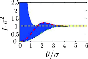
Figure 2: Fisher informations versus the parameter $\theta$. The blue region represents the set of curves of $I(\hat{\rho}_{\mathrm{ps}}^{\mathcal{K}})$, while the yellow dashed line indicates $I(\hat{\rho}_{\mathrm{int}}^{\mathcal{H}\otimes\mathcal{K}})$. The red dashed-dotted and green dotted lines show the classical Fisher information $I_{\mathrm{c}}(f_{\rm ps}(x))$ with $c=1$ and $c=-1$, respectively.

IV Comparing estimation errors in asymptotic condition

In the last section, we have seen that the sensitivity of the state to the parameter $\theta$ can be enhanced via the postselection. This would suggest, as shown in Eq. (2), that the postselection can bring about further decrease of the Cramér-Rao bound, i.e, the strict lower bound of the estimation error of $\theta$. However, the critical issue with this postselection technique is that we obtain the state only when the postselection succeeds; that is, we have to construct the estimator using less measurement data, compared to the standard method based on the whole state $\hat{\rho}^{\mathcal{H}\otimes\mathcal{K}}_{\mathrm{int}}$. Therefore, the problem becomes comparing the Cramér-Rao bounds $1/n_{\rm ps}I(\hat{\rho}_{\mathrm{ps}}^{\mathcal{K}})$ and $1/n_{\rm int}I(\hat{\rho}^{\mathcal{H}\otimes\mathcal{K}}_{\mathrm{int}})$, where $n_{\rm ps}$ and $n_{\rm int}$ are the number of trials in those methods, respectively.

The above problem is not straightforward to solve. However, if we are allowed to perform the trial infinitely many times, it is possible to have a general answer. In fact, in such asymptotic condition, there exist estimators attaining the Cramér-Rao bounds Nagaoka ; Fujiwara_MLE , and furthermore, the number of trials are explicitly given by $n_{\rm ps}={\rm Pr}(f)n$ and $n_{\rm int}=n$, as was also discussed in Knee . Hence, the problem is now to compare ${\rm Pr}(f)I(\hat{\rho}_{\mathrm{ps}}^{\mathcal{K}})$ and $I(\hat{\rho}^{\mathcal{H}\otimes\mathcal{K}}_{\mathrm{int}})$.

To solve the problem, let us define

$$\tilde{B}:=\mbox{}_{\cal H}\langle{f}|e^{-i\theta(\hat{H}-\langle{\hat{H}}\rangle)}|{i}\rangle_{\mathcal{H}},$$ (13)

where $\langle{\hat{H}}\rangle={\rm Tr}\hskip 1.9919pt(\hat{\rho}_{\mathrm{int}}^{\mathcal{H}\otimes\mathcal{K}}\hat{H})$, which leads to

$$\hat{\rho}^{\mathcal{K}}_{\mathrm{ps}}=\tilde{B}\hat{\rho}_{i}^{\mathcal{K}}\tilde{B}^{\dagger}/{\rm Tr}(\tilde{B}\hat{\rho}_{i}^{\mathcal{K}}\tilde{B}^{\dagger}),~{}~{}{\rm Pr}\left({f}\right)=\langle{\psi}|\tilde{B}^{\dagger}\tilde{B}|{\psi}\rangle.$$

Then, since $|{f}\rangle_{\mathcal{H}}\langle{f}|\otimes I^{\mathcal{K}}\leq\hat{I}^{\mathcal{H}\otimes\mathcal{K}}$, we have

$${\rm Pr}\left({f}\right)I(\hat{\rho}_{\mathrm{ps}}^{\mathcal{K}})/4$$

$$=\langle{\psi}|\partial_{\theta}\tilde{B}^{\dagger}\partial_{\theta}\tilde{B}|{\psi}\rangle-\frac{\bigl{|}\langle{\psi}|\partial_{\theta}\tilde{B}^{\dagger}\tilde{B}|{\psi}\rangle\bigr{|}^{2}}{\langle{\psi}|\tilde{B}^{\dagger}\tilde{B}|{\psi}\rangle}$$

$$\leq\langle{\psi}|\partial_{\theta}\tilde{B}^{\dagger}\partial_{\theta}\tilde{B}|{\psi}\rangle$$

$$=\mbox{}_{\mathcal{K}}\langle{\psi}|\mbox{}_{\mathcal{H}}\langle{i}|(\hat{H}-\langle{\hat{H}}\rangle)e^{-i\theta(\hat{H}-\langle{\hat{H}}\rangle)}|{f}\rangle_{\mathcal{H}}$$

$$~{}~{}~{}~{}~{}~{}~{}\times\mbox{}_{\mathcal{H}}\langle{f}|(\hat{H}-\langle{\hat{H}}\rangle)e^{i\theta(\hat{H}-\langle{\hat{H}}\rangle)}|{i}\rangle_{\mathcal{H}}|{\psi}\rangle_{\mathcal{K}}$$

$$\leq\langle{i,\psi}|(\hat{H}-\langle{\hat{H}}\rangle)^{2}e^{-i\theta(\hat{H}-\langle{\hat{H}}\rangle)}e^{i\theta(\hat{H}-\langle{\hat{H}}\rangle)}|{i,\psi}\rangle$$

$$=\langle{i,\psi}|(\hat{H}-\langle{\hat{H}}\rangle)^{2}|{i,\psi}\rangle=I(\hat{\rho}_{\mathrm{int}}^{\mathcal{H}\otimes\mathcal{K}})/4.$$

As a result,

$${\rm Pr}\left({f}\right)I\bigl{(}\hat{\rho}_{\mathrm{ps}}^{\mathcal{K}}\bigr{)}\leq I\bigl{(}\hat{\rho}_{\mathrm{int}}^{\mathcal{H}\otimes\mathcal{K}}\bigr{)}.$$ (14)

Therefore, we now obtain a general answer to the question considered throughout the paper; in the asymptotic condition, the postselection method does never yield a better estimator that outperforms the standard method that allows us to perform any measurement on the whole composite system. Within the context of quantum metrology mentioned at the beginning of Sec. I, this fact has the following interpretation. Again, the problem is to estimate the unknown parameter $\theta$ contained in the given system ${\cal S}$ in the form $\hat{U}=\exp(-i\theta\hat{H})$. Then, the weak-value amplification techniques found in the literature suggest us to divide the system into two parts ${\cal H}$ and ${\cal K}$, perform a suitable postselection on ${\cal H}$, and then detect a rare event on ${\cal K}$, which would contain valuable information about $\theta$. However, the inequality (14) implies that this strategy does not have an advantage in estimating $\theta$ for any partitioning of the given system ${\cal S}$ into two subsystems, ${\cal S}={\cal H}\otimes{\cal K}$, and for any type of postselection on ${\cal H}$. In this sense, the inequality (14) is a no-go theorem in the field of quantum metrology.

V Discussion

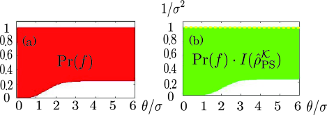
Figure 3: (a) The success probability ${\rm Pr}(f)$ and (b) Fisher information normalized by ${\rm Pr}(f)$, as functions of $\theta/\sigma$. The regions represent the set of curves of ${\rm Pr}(f)$ and $\Pr(f)I(\hat{\rho}_{\mathrm{ps}}^{\mathcal{K}})$ generated with various values of $(t_{1},t_{2},s_{1}-s_{2})$.

The main conclusion we have obtained is that, in general, the signal amplification technique based on the weak measurement or more broadly the postselection is useless in the statistics sense. Note again that this result is obtained under asymptotic condition; in other words, when the measurement can be carried out only finite times, ${\rm Pr}(f)n$ does not anymore have the meaning of the number of success of the postselection, and it is not clear whether or not a similar inequality holds. Actually we have the following fact: Let us reconsider the example studied in Sec III. Figure 3 shows the success probability ${\rm Pr}(f)$ and the Fisher information normalized by ${\rm Pr}(f)$. In the right panel, the yellow dashed line shows $I(\hat{\rho}_{\mathrm{int}}^{\mathcal{H}\otimes\mathcal{K}})=1/\sigma^{2}$. This figure demonstrates that, by performing a suitable postselection, it is possible to attain nearly the equality in Eq. (14) for almost all $\theta$; hence, it seems that such a fine postselection could realize $n_{\rm ps}I(\hat{\rho}_{\mathrm{ps}}^{\mathcal{K}})>n_{\rm int}I(\hat{\rho}^{\mathcal{H}\otimes\mathcal{K}}_{\mathrm{int}})$ for finite numbers of trial $n_{\rm ps}$ and $n_{\rm int}$. However, Ferrie and Combes proved in Ferrie that this conjecture does not hold; that is, the postselection does not enhance the precision of the parameter estimate for any amount of data. We also should point out the recent preprint Knee 2013 by Knee and Gauger, which proves no advantage of the postselection-based amplification technique in a slightly different setting.

Another important question is about how to experimentally demonstrate the inequality (14). To achieve this goal, we need to construct a system such that we can measure the whole system globally for computing $I(\hat{\rho}_{\mathrm{int}}^{\mathcal{H}\otimes\mathcal{K}})$ as well as each subsystem locally for computing $I(\hat{\rho}_{\mathrm{ps}}^{\mathcal{K}})$. For instance a pair of trapped ions, which corresponds to $\mathcal{H}\otimes\mathcal{K}$, fulfills these requirements; actually, Riebe, et al. showed in experiment that it is possible to couple two trapped calcium ions, manipulate each ion individually, and perform a complete global (Bell) measurement by detecting fluorescence from the ions. On the other hand, for instance a nano-mechanical oscillator ($\mathcal{H}$) driven by optical force with unknown strength $\theta$, which arises due to the interaction between the oscillator and an environment field ($\mathcal{K}$), is not a suitable system for the experimental demonstration, because in this case the environment field is not accessible. Here we remark that this issue further raises the following important questions: Can we apply the postselection technique to estimate unknown parameters of an open system? If this is the case, does the postselection offer any advantage? Parameter estimation problems for an open system now constitute an important research area Mankei , so the applicability of the postselection technique should be explored.

References

• (1) V. Giovannetti, S. Lloyd, and L. Maccone, Science 306, pp.1330-1336 (2004), Phys. Rev. Lett. 96, 010401 (2006).
• (2) Y. Aharonov, D. Z. Albert, and L. Vaidman, Phys. Rev. Lett. 60, 1351 (1988), Y. Aharonov and A. Botero, Phys. Rev. A 72, 052111 (2005), Y. Aharanov and D. Rohrlich, Quantum Paradoxes (Wiley-VCH, Weinheim, 2005).
• (3) R. Jozsa, Phys. Rev. A 76, 044103 (2007).
• (4) O. Hosten and P. Kwiat, Science 319, 787 (2008).
• (5) P. B. Dixson, D. J. Starling, A. N. Jordan, and J. C. Howell, Phys. Rev. Lett. 102, 173601 (2009).
• (6) S. Wu and Y. Li, Phys. Rev. A 83, 052106 (2011).
• (7) T. Koike and S. Tanaka, Phys. Rev. A 84, 062106 (2012).
• (8) K. Nakamura, A. Nishizawa, and M. Fujimoto, Phys. Rev. A 85, 012113 (2012).
• (9) A. Nishizawa, K. Nakamura, and M. Fujimoto, Phys. Rev. A 85, 062108 (2012).
• (10) Y. Susa, Y. Shikano, and A. Hosoya, Phys. Rev. A 85, 052110 (2012).
• (11) J. Lee and I. Tsutsui, arXiv:1305.2721
• (12) C. W. Helstrom, Quantum Detection and Estimation Theory (Academic, New York, 1976).
• (13) A. S. Holevo, Probabilistic and Statistical Aspects of Quantum Theory (North-Holland, Amsterdam, 1982).
• (14) S. L. Braunstein and C. M. Caves, Phys. Rev. Lett. 72, 3439 (1994).
• (15) A. S. Holevo, Statistical Structure of Quantum Theory (Berlin, Springer, 2001).
• (16) M. Hayashi, Quantum Information: An Introduction (Berlin, Springer, 2006).
• (17) H. Nagaoka, Asymptotic Theory of Quantum Statistical Inference ed. M. Hayashi (Singapore, World Scientific, 2005) pp.125-132.
• (18) A. Fujiwara, J. Phys. A: Math. Gen, 39, 12489 (2006).
• (19) G. C. Knee, G. A. D. Briggs, S. C. Benjamin, and E. M. Gauger, Phys. Rev. A 87, 012115 (2013).
• (20) H. F. Hofmann, AIP Conf. Proc. 1363, 125 (2011), Phys. Rev. A 83, 022106 (2011); H. F. Hofmann, M. E. Goggin, M. P. Almeida, and M. Barbieri, Phys. Rev. A 86, 040102(R) (2012).
• (21) Y. Shikano and S. Tanaka, Europhys. Lett. 96, 40002 (2011).
• (22) G. Strubi and C. Bruder, Phys. Rev. Lett. 110, 083605 (2013).
• (23) G. I. Viza, et. al., Opt. Lett. 38, 2949 (2013).
• (24) C. Ferrie and J. Combes, arXiv:1307.4016 (2013).
• (25) G. C. Knee and E. M. Gauger, arXiv:1306.6321 (2013).
• (26) M. Riebe, et. al., Nature 429, 734 (2004).
• (27) M. Tsang, New J. Phys. 15, 073005 (2013).