Canonical Labelling of Site Graphs

Abstract

We investigate algorithms for canonical labelling of site graphs, i.e. graphs in which edges bind vertices on sites with locally unique names. We first show that the problem of canonical labelling of site graphs reduces to the problem of canonical labelling of graphs with edge colourings. We then present two canonical labelling algorithms based on edge enumeration, and a third based on an extension of Hopcroft’s partition refinement algorithm. All run in quadratic worst case time individually. However, one of the edge enumeration algorithms runs in sub-quadratic time for graphs with "many" automorphisms, and the partition refinement algorithm runs in sub-quadratic time for graphs with "few" bisimulation equivalences. This suite of algorithms was chosen based on the expectation that graphs fall in one of those two categories. If that is the case, a combined algorithm runs in sub-quadratic worst case time. Whether this expectation is reasonable remains an interesting open problem.

1 Introduction

Graphs are widely used for modelling in biology. This paper focuses on graphs for modelling protein complexes: vertices correspond to proteins, and edges correspond to bindings. Moreover, vertices are labelled by protein names, and edges connect vertices on labelled sites, giving rise to a notion of site graphs. Importantly, site labels can be assumed to be unique within vertices, i.e. a protein can have at most one site of a given name. This uniqueness assumption introduces a level of rigidity which can be exploited in algorithms on site graphs. Rigidity is for example crucial for containing the computational complexity of one algorithm for stochastic simulation of rule-based models of biochemical signalling pathways [3].

In this paper we investigate how rigidity can be exploited in the design of efficient algorithms for canonical labelling of site graphs. Informally, a canonical labelling procedure must satisfy that the canonical labellings of two graphs are identical if and only if the two graphs are isomorphic. A graph isomorphism is understood in the usual sense of being an edge-preserving bijection, with the additional requirement that vertex and site labellings are also preserved. Hence two site graphs are isomorphic exactly when they represent protein complexes belonging to the same species. The graph isomorphism problem on general graphs is hard: it is not known to be solvable in polynomial time, but curiously is not known to be NP-complete either even though it is in NP [10]. The canonical labelling problem clearly reduces to the graph isomorphism problem, but there is no clear reduction the other way. In this sense the canonical labelling problem is harder than the graph isomorphism problem.

Efficient canonical labelling of site graphs has an application in a second algorithm for stochastic simulation of rule-based languages [7]. This algorithm at frequent intervals determines isomorphism of a site graph, representing a newly created species, with a potentially large number of site graphs representing all other species in the system at a given point in time. The algorithm can hence compute a canonical labelling when a new species is first created, and subsequently determine isomorphism quickly by checking equality between this and existing canonical labellings.

We assume in this paper that the number of site labels and the degree of vertices in site graphs are bounded, i.e. they do not grow asymptotically with the number of vertices, which indeed appears to be the case in the biological setting. An algorithm for site graph isomorphism is presented in [9] and has a worst-case time complexity of $O(\lvert V\rvert^{2})$, where $V$ is the set of vertices. In this paper we exploit similar ideas, based on site uniqueness, in the design of new algorithms for canonical labelling, which also have a worst-case time complexity of $O(\lvert V\rvert^{2})$. We furthermore characterise the graphs for which lower complexity bounds are possible: if the bisimulation equivalence classes are “small”, meaning $O(1)$, or if the automorphism classes are “large”, meaning $O(\lvert V\rvert)$, then an $O(\lvert V\rvert\cdot\log\lvert V\rvert)$ time complexity can be achieved in worst and average case, respectively.

Site graphs can be encoded in a simpler, more standard notion of graphs with edge-colourings. We formally define these graphs in Section 2, along with the notion of canonical labelling and other preliminaries. In Section 3 we specify two canonical labelling algorithms based on ordered edge enumerations, and in Section 4 we show how these algorithms can be improved using partition refinement. We conclude in Section 5.

2 Preliminaries

2.1 Notation

We write $X\rightarrow Y$ (respectively $X\rightarrow_{\text{{bij}}}Y)$ for the set of total functions (respectively total bijective functions) from $X$ to $Y$. We use the standard notation $\prod x\in X.\,T(x)$ for dependent products, i.e. the set of total functions which map an $x\in X$ to some $y\in T(x)$. We write $\operatorname{Dom}(f)$ and $\operatorname{Im}(f)$ for the domain of definition and image of $f$, respectively, and $f\downarrow\text{Z}$ for the restriction of $f$ to the domain $Z$. We view functions as sets of pairs $(x\mapsto y)$ when notationally convenient. We use standard notation for finite multisets, and use the brackets $\{\mid\cdot\mid\}$ for multiset comprehension. We write $\mathcal{T}(X)$ for the set of total orders on $X$. We write $X^{*}$ for the Kleene closure of $X$, i.e. the set of finite strings over the symbols in $X$. Given a linearly ordered set $(X,<)$ we assume the lexicographic extension of $<$ to pairs and lists over $X$. Given a partially ordered set $(X,<)$ we write $\min_{<}(X)$ for the set of minimal elements of $X$ under $<$, and if the ordering is total we identify $\min_{<}(X)$ with its unique least element. Given an equivalence relation $\rho$ on a set $X$ and $x\in X$, we write $[x]_{\rho}$ for the equivalence class of $x$ under $\rho$, and we write $X^{\prime}/\rho$ for the partition of $X^{\prime}\subseteq X$ under $\rho$. Finally, given a list $x$, we write $x.i$ for the $i$th element of $x$ starting from $1$.

2.2 Site Graphs and Coloured Graphs

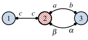
(a) A site graph.

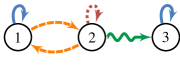
(b) A coloured graph.

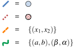
(c) Colour definitions.

Figure 2.1: An example of a site graph (a), its encoding as a coloured graph (b), and the formal definition of colours (c) following the encoding in Appendix A with the site name ordering $a{\,\preceq_{\text{s}}\,}b{\,\preceq_{\text{s}}\,}c{\,\preceq_{\text{s}}\,}\alpha{\,\preceq_{\text{s}}\,}\beta$. The direction of e.g. the edge $(2,3)$ is determined by $a{\,\preceq_{\text{s}}\,}b$ and $(a,b)$ being the minimum pair of connected sites between vertices $2$ and $3$.

A site graph is a multi-graph with vertices labelled by protein names and edges which connect vertices on sites labelled by site names. An example is shown in Figure 2.1a where protein names are indicated by colours, and a formal definition is given in Appendix A, Definition 16. From an algorithmic perspective, the key property of site graphs is their rigidity: a vertex can have at most one site of a given name, so a site name uniquely identifies an adjacent edge. This rigidity property can be captured by the simpler, more standard notion of directed graphs with edge-colourings. An example is shown in Figure 2.1b, and the formal definition follows below.

Definition 1.

Let $(\Sigma,\prec)$ be a given linearly ordered set of edge colours. Then $\mathcal{CG}$ is the set of all edge coloured graphs $G=(V,E,\phi)$ where:

• $V=\{1,\dots,k\}$ is a set of vertices.

• $E\subseteq V\times V$ is a set of directed edges.

• $\phi:E\rightarrow\Sigma$ is an edge colouring satisfying for all $v\in V$ that $\phi\downarrow\{(v,v^{\prime})\in E\}$ and $\phi\downarrow\{(v^{\prime},v)\in E\}$ are injective.

Given a coloured graph $G$, we write $V_{{G}}$, $E_{{G}}$ and $\phi_{G}$ for the vertices, edges and edge colouring of $G$, respectively. We write $\text{Adj}(v)$, respectively $\text{Adj}^{-1}(v)$, for the set of all outgoing, respectively incoming, edges adjacent to $v$. We measure the size of graphs as the sum of the number of edges and vertices, i.e. $\lvert G\rvert\leavevmode\nobreak\ \overset{\Delta}{\simeq}\leavevmode\nobreak\ \lvert V_{{G}}\rvert+\lvert E_{{G}}\rvert$. Since we assume the degree of vertices to be bounded, we have that $O(\lvert G\rvert)=O(\lvert V_{{G}}\rvert)=O(\lvert E_{{G}}\rvert)$.

The condition on edge colours states that a vertex can have at most one incident edge of a given colour, thus capturing the rigidity property. We give an encoding of site graphs into coloured graphs in Appendix A. The encoding is injective, respects isomorphism, and is linear in size and time (Proposition 18 in Appendix A). It hence constitutes a reduction from the site graph isomorphism problem to the coloured graph isomorphism problem. This allows us to focus exclusively on coloured graphs in the following. Since we are interested in protein complexes, we furthermore assume that the underlying undirected graphs are always connected. Figure 2.1b is in fact an example encoding of Figure 2.1a, with the specific choice of colours used by the encoding shown in Figure 2.1c.

2.3 Isomorphism and Canonical Labelling

Our notion of coloured graph isomorphism is standard. In addition to preserving edges, isomorphisms must preserve edge colours.

Definition 2.

Let $G$ and $G^{\prime}$ be coloured graphs. An isomorphism is a bijective function $\sigma:V_{{G}}\rightarrow_{\text{{bij}}}V_{{G^{\prime}}}$ satisfying that $\sigma(G)=G^{\prime}$, i.e.:

• $\forall v_{1},v_{2}\in V_{{G}}.\,[(v,v_{2})\in E_{{G}}\Leftrightarrow(\sigma(v_{1}),\sigma(v_{2}))\in E_{{G^{\prime}}}]$.

• $\forall e\in E_{{G}}.\,\phi_{G}(e)=\phi_{G^{\prime}}(\sigma(e))$.

Furthermore define $G\simeq G^{\prime}$ ($G$ and $G^{\prime}$ are isomorphic) iff there exists an $\sigma$ relating $G$ and $G^{\prime}$, and define $(G,v)\simeq(G^{\prime},v^{\prime})$ (or simply $v\simeq v^{\prime}$) iff there exists an $\sigma$ s.t. $\sigma(v)=v^{\prime}$. We denote by $I(G,G^{\prime})$ the set of isomorphisms from $G$ to $G^{\prime}$. An isomorphism from $G$ to itself is called an automorphism.

Since all graphs of the same size have the same vertices, all isomorphisms are in fact automorphisms. We next define our notion of canonical labelling. Having vertices given by integers allows the canonical labelling of a graph to be a graph itself.

Definition 3.

A canonical labeller is a function $L:\prod G\in\mathcal{CG}.\,[G]_{\simeq}$ satisfying for all $G,G^{\prime}\in\mathcal{CG}$ that $L(G)=L(G^{\prime})\Leftrightarrow G\simeq G^{\prime}$. We say that $L(G)$ is a canonical labelling of $G$, and that $G$ is canonical if $L(G)=G$.

3 Edge Enumeration Algorithms

This section introduces two algorithms based on enumeration of edges and the comparison of these enumerations.

3.1 Edge Enumerators

The rigidity property of coloured graphs, together with the linear ordering of colours, means that any given initial node uniquely identifies an enumeration of all the edges in a graph. Such an enumeration can be obtained by traversing the graph from the initial node while always following edges according to the given linear ordering on colours. There are many possible enumeration procedures, so we generalise the notion of an edge enumerator as follows.

Definition 4.

An edge enumerator is a function of the form $\eta:\prod G\in\mathcal{CG}.\,V_{{G}}\rightarrow\mathcal{T}(E_{{G}})\times(V_{{G}}\rightarrow_{\text{{bij}}}V_{{G}})$ satisfying for all $G,G^{\prime}$ and $v\in V_{{G}},v^{\prime}\in V_{{G^{\prime}}}$ with $v\simeq v^{\prime}$, $\eta(G,v)=(\lhd,\alpha)$ and $\eta(G^{\prime},v^{\prime})=(\lhd^{\prime},\alpha^{\prime})$ that $\alpha(G,\lhd)=\alpha^{\prime}(G^{\prime},\lhd^{\prime})$.

input : a graph $G$ and a start vertex $v\in V_{{G}}$

output : an enumeration of the edges in $G$ from $v$

1 $\text{Enum}\leftarrow[]$ /* a list of enumerated edges */

2 $\alpha\leftarrow\{(v\rightarrow 1)\}$ /* a vertex renaming identifying order of encounter */

3 $Q\leftarrow\text{Queue}(v)$ /* a queue initialised with $v$ */

4 Visited $\leftarrow\{v\}$ /* a set of visited vertices */

5 while $Q$ is not empty do

6       $v\leftarrow$ Dequeue($Q$)

7       outEdges $\leftarrow\text{Sort}_{\prec}(\text{Adj}(v))$

8       inEdges $\leftarrow\text{Sort}_{\prec}(\text{Adj}^{-1}(v))$

9       edges $\leftarrow$ outEdges$@$inEdges

10       for $i=1$ to $\lvert\emph{edges}\rvert$ do

11             $(v_{1},v_{2})\leftarrow\text{edges}.i$

12             if $(v_{1},v_{2})$ does not occur in Enum then

13                   $\text{Enum}\leftarrow(v_{1},v_{2})::\text{Enum}$

14                   $v_{\text{new}}\leftarrow v_{1}\text{ if }v=v_{2}$ and $v_{2}$ if $v=v_{1}$

15                   if $v_{\text{new}}\not\in\emph{Visited}$ then

16                         $\text{Visited}\leftarrow\text{Visited}\cup\{v_{\text{new}}\}$

17                         $\alpha\leftarrow\alpha\cup\{(v_{\text{new}}\mapsto\lvert\text{Visited}\rvert)\}$

18                         Enqueue($Q,v_{\text{new}}$)

19                        

20                  

21            

22      

23return (Enum, $\alpha$)

Algorithm 1 An edge enumeration algorithm. We assume given an operator $\text{Sort}_{\prec}(X)$ which sorts the set $X$ according to a linear ordering $\prec$. The operators $::$ and $@$ are list cons and append, respectively.

An edge enumerator must hence produce a linear ordering of edges and an alpha-conversion, with the key property that the alpha-converted graph is invariant under isomorphism. A more direct definition is possible, but we require the alpha-conversion to be given explicitly by the enumerator for use in subsequent algorithms. We get the following directly from the definition of edge enumerators.

Lemma 5.

Let $\eta$ be an edge enumerator and let $\eta(G,v)=(\lhd,\alpha)$ and $\eta(G^{\prime},v^{\prime})=(\lhd^{\prime},\alpha^{\prime})$ for some $G,G^{\prime}$ and $v,v^{\prime}$. If $\alpha(G)=\alpha(G^{\prime})$ then $(G,v)\simeq(G,v^{\prime})$.

Algorithm 1 implements an edge enumerator. It essentially carries out a breadth first search (BFS) on the underlying undirected graph: edges are explored in order of colour, but with out-edges arbitrarily explored before in-edges (lines $7$-$9$). The inner loop checks whether an edge has been encountered previously (line $12$) in order to avoid an edge being enumerated twice. The generated alpha-conversion renames vertices by their order of discovery by the algorithm (line $17$).

Proposition 6.

Algorithm 1 computes an edge enumerator.

The intuition of the proof is that the control flow of the algorithm does not depend on vertex identity, and hence the output should indeed be invariant under automorphism. The full proof is by induction in the number of inner loop iterations. For the complexity analysis observe that the algorithm is essentially a BFS which hence runs in $O(\lvert V_{{G}}\rvert+\lvert E_{{G}}\rvert)$ time, which by assumption is $O(\lvert V_{{G}}\rvert)$ in our case. The extensions do not affect this complexity bound, assuming that the checks for containment of elements in Visited and Enum are $O(1)$; this is possible using hash map implementations.

3.2 A Pair-Wise Canonical Labelling Algorithm

Alpha-converted edge enumerations can be ordered lexicographically based on edge identity firstly, and on edge colours secondly. This ordering is defined formally as follows.

Definition 7.

Define a linear order $\sqsubset$ on coloured edges as $(e,c)\sqsubset(e^{\prime},c^{\prime})$ iff $e<e^{\prime}\lor(e=e^{\prime}\land c\prec c^{\prime})$. We extend the order to pairs $(G,e)$ s.t. $(G,e)\sqsubset(G^{\prime},e^{\prime})$ iff $(e,\phi_{G}(e))\sqsubset(e^{\prime},\phi_{G^{\prime}}(e^{\prime}))$. Finally, we assume the lexicographic extension of $\sqsubset$ to pairs $(G,\lhd),(G^{\prime},\lhd^{\prime})$ of edge-ordered graphs.

The ordering is used for canonical labelling by Algorithm 2, which essentially finds the edge enumeration from each vertex in the input graph, picks the smallest after alpha-conversion, and applies the associated alpha-conversion to the graph. Whenever two alpha-converted enumerations are identical (line $11$), the source vertices are isomorphic by definition of edge enumerators. The isomorphism is then computed (line $12$) and the set of pending vertices is filtered so that it contains at most one element from each pair of isomorphic vertices (lines $13$-$20$). If both elements of a pair of isomorphic vertices are in the set of pending vertices, one element is removed from the pending set (lines $16$-$17$); the least element under $<$ is chosen arbitrarily, which ensures that the other element does not get removed at a later iteration. If just one element of the pair is in the pending set (lines $18$-$19$), the other element must have been visited earlier, and so the present pending element can be safely removed.

input : a graph $G$ and an edge enumerator $\eta$

output : a canonical labelling of $G$

1 $V_{\text{pending}}\leftarrow$ $V_{{G}}$ /* vertices yet to be enumerated */

2 $\lhd_{\text{min}}\leftarrow$ null /* the least ordering */

3 $\alpha_{\text{min}}\leftarrow$ null /* the least alpha-conversion */

4 while $V_{\text{pending}}\neq\emptyset$ do

5       $v\leftarrow$ any $v\in V_{\text{pending}}$

6       $V_{\text{pending}}\leftarrow V_{\text{pending}}\setminus{v}$

7       $(\lhd,\alpha)\leftarrow\eta(G,v)$

8       if ($\lhd_{\text{min}}$ = $\alpha_{\text{min}}$ = null) or ($\alpha(G,\lhd)\sqsubset\alpha_{\text{min}}(G,\lhd_{\text{min}})$) then

9             $\lhd_{\text{min}}\leftarrow\lhd$

10             $\alpha_{\text{min}}\leftarrow\alpha$

11            

12      else if $\alpha(G,\lhd)=\alpha_{\text{min}}(G,\lhd_{\text{min}})$ then

13             $a\leftarrow\alpha_{\text{min}}^{-1}\circ\alpha$ /* find the automorphism */

14             $V^{\prime}_{\text{pending}}\leftarrow V_{\text{pending}}$ /* keep a copy of pending vertices */

15             for $v^{\prime}\in\operatorname{Dom}(\alpha)$ do

16                   /* discard isomorphic vertices from pending */

17                   if $\{v,\alpha(v)\}\subseteq V_{\text{pending}}$  then

18                         $V^{\prime}_{\text{pending}}\leftarrow V_{\text{pending}}\setminus\text{Min}_{<}\{v,\alpha(v)\}$

19                        

20                  else

21                         $V^{\prime}_{\text{pending}}\leftarrow V_{\text{pending}}\setminus\{v,\alpha(v)\}$

22                        

23                  

24            $V_{\text{pending}}\leftarrow V^{\prime}_{\text{pending}}$

25            

26      

27return $\alpha_{\text{min}}(G)$

Algorithm 2 A pair-wise canonical labelling algorithm.

Proposition 8.

Algorithm 2 is a canonical labeller.

The worst-case time complexity of Algorithm 2 is $O(\lvert V_{{G}}\rvert^{2})$, namely when no vertices are isomorphic. If all nodes in the input graph are isomorphic, the number of pending vertices is halved at every iteration of the outer loop and hence the complexity is $O(\lvert V_{{G}}\rvert\cdot\log(\lvert V_{{G}}\rvert)).$ More generally, this bound also holds in the average case if the largest automorphism equivalence class has size $O(\lvert V_{{G}}\rvert)$. There are several ways of improving the algorithm. One way is to further exploit automorphisms. When new automorphisms are found, these may generate additional automorphisms through composition with existing ones. In addition to removing elements of the pending set, automorphisms could also be exploited by only considering the automorphism quotient graph in subsequent iterations. Another way of improving the algorithm is to compute edge enumerations lazily, up until the point where they can be distinguished from the current minimum. Neither of the above improvements, however, change the worst case complexity characteristics of the algorithm.

3.3 A Parallel Canonical Labelling Algorithm

The idea of lazily enumerating edges can be taken a step further with a second algorithm which enumerates edges from all nodes in parallel: at each iteration, a single edge is emitted by each enumeration. Following standard notions of lazy functions, we formally define the notion of a lazy edge enumerator below, where the singleton set $\{*\}$ corresponds to the unit type.

Definition 9.

For each coloured graph $G$ and $i\in\{0\dots\lvert E_{{G}}\rvert-1\}$, define the set of functions $T_{i}(G)\leavevmode\nobreak\ \overset{\Delta}{\simeq}\leavevmode\nobreak\$ $\{*\}\rightarrow E_{{G}}\times V_{{G}}\times V_{{G}}\times T_{i+1}$ with $T_{\lvert E_{{G}}\rvert}\leavevmode\nobreak\ \overset{\Delta}{\simeq}\leavevmode\nobreak\ \mathcal{CG}$. A lazy edge enumerator implementing a given enumerator $\eta$ is then a function ${\eta_{\text{L}}}:\prod G\in\mathcal{CG}.\,V_{{G}}\rightarrow T_{0}(G)$ satisfying for any $G$ and $v\in V_{{G}}$ with $\eta(G,v)=(\lhd,\alpha)$ that $(E_{{G}},\lhd).i=e_{i}$, $\alpha(e_{i})=(v_{i},v_{i}^{\prime})$ and ${\eta_{\text{L}}}_{\lvert E_{{G}}\rvert}=\alpha(G)$ where $(e_{i},v_{i},v_{i}^{\prime},{\eta_{\text{L}}}_{i})\leavevmode\nobreak\ \overset{\Delta}{\simeq}\leavevmode\nobreak\ {\eta_{\text{L}}}_{i-1}(*)$ for $i\in\{1\dots\lvert E_{{G}}\rvert\}$ and ${\eta_{\text{L}}}_{0}\leavevmode\nobreak\ \overset{\Delta}{\simeq}\leavevmode\nobreak\ {\eta_{\text{L}}}(G,v)$.

Hence a lazy edge enumerator produces, given a graph and a start vertex, a function which can be applied to yield an edge, an alpha-conversion of the edge (i.e. two vertices) and a continuation which in turn can be applied in a similar fashion; the final function thus applied yields an alpha-converted graph for notational convenience below. A lazy version of the BFS edge enumerator in Algorithm 1 can be implemented in a straightforward manner in a functional language. This does not affect the complexity characteristics of the algorithm, i.e. it still runs in $O(\lvert V_{{G}}\rvert)$ time.

Algorithm 3 computes canonical labellings using lazy edge enumerators. It first initialises a set of enumerators from each vertex in the input graph (line $1$). It then enters a loop in which enumerators are gradually filtered out, terminating when the remaining enumerators complete with an alpha-converted graph. At termination, all remaining enumerators will have started from isomorphic vertices, and hence they all evaluate in their last step to the same alpha-converted graph. At each iteration, each enumerator takes a step, yielding the next version of itself and an alpha-converted coloured edge; the result is stored as a mapping from the former to the latter (line $3$). A multiset of alpha-converted, coloured edges is then constructed for the purpose of counting the number of copies of each alpha-converted coloured edge (line $4$). The alpha-converted coloured edges with the smallest multiplicity are selected, and of these the least under $\sqsubset$ is selected (lines $5$-$6$). Only the enumerators which yielded this selected edge are retained in the new set of pending edge enumerators (line $7$). Note that further discrimination according to connectivity with other enumerators would be possible: for example, the vertices which are sources of enumerators eliminated in step $n$ could be distinguished from those which are sources of enumerators eliminated in step $m\neq n$. We have omitted this for simplicity.

input : a graph $G$ and a lazy edge enumerator ${\eta_{\text{L}}}$

output : a canonical labelling of $G$

1 Pending $\leftarrow\{{\eta_{\text{L}}}(G,v)\mid v\in V_{{G}}\}$

2 while $\text{Pending}\not\subset\mathcal{CG}$ do

3       StepMap $\leftarrow\{{\eta_{\text{L}}}^{\prime}\mapsto((v,v^{\prime}),\phi_{G}(e))\mid(e,v,v^{\prime},{\eta_{\text{L}}}^{\prime})={\eta_{\text{L}}}(*)\land{\eta_{\text{L}}}\in Pending\}$

4       Steps $\leftarrow\{\mid\text{StepMap}({\eta_{\text{L}}}^{\prime})\mid{\eta_{\text{L}}}^{\prime}\in\operatorname{Dom}(\text{StepMap})\mid\}$

5       SmallestMult $\leftarrow\min_{<}\{\text{Steps}(e,c)\mid(e,c)\in\text{Steps}\}$

6       LeastEdge $\leftarrow\min_{\sqsubset}\{(e,c)\in\text{Steps}\mid\text{Steps}(e,c)=\text{SmallestMult}\}$

7       Pending $\leftarrow\{{\eta_{\text{L}}}^{\prime}\in\operatorname{Dom}(\text{StepMap})\mid\text{StepMap}({\eta_{\text{L}}}^{\prime})=\text{LeastEdge}\}$

8      

9return the one member of Pending

Algorithm 3 A parallel canonical labelling algorithm.

Proposition 10.

Algorithm 3 is a canonical labeller.

The initialisation in line $1$ runs in $O(\lvert V_{{G}}\rvert)$ time. The loop always requires $\lvert E_{{G}}\rvert=O(\lvert V_{{G}}\rvert)$ iterations. In the worst case where all vertices are isomorphic, each line within the loop requires $O(\lvert V_{{G}}\rvert)$ time, so the worst case complexity is $O(\lvert V_{{G}}\rvert^{2})$. Hence in the worst case there is no asymptotic improvement over Algorithm 2. In practice, however, Algorithm 3 is likely to perform significantly better.

The key question is how Algorithm 3 behaves in cases where there are few automorphisms, i.e. when the number of automorphisms is sub-linear in the number of vertices. One can hypothesise that asymmetry is then discovered sufficiently early to yield an $O(\lvert V_{{G}}\rvert\cdot\log(\lvert V_{{G}}\rvert))$ time complexity. If so, an overall $O(\lvert V_{{G}}\rvert\cdot\log(\lvert V_{{G}}\rvert))$ algorithm is obtained by running the pairwise and the parallel algorithms simultaneously, terminating when the first of the two algorithms terminates. However, this question remains open. Therefore also the question of whether a sub-quadratic time complexity bound exists in the general case remains open.

4 A Partition Refinement Algorithm

The vertex set of a coloured graph can be partitioned based on “local views”: vertices with the same colours of incident edges are considered equivalent and are hence included in the same equivalence class of the partition. If two vertices are in different classes, they are clearly not isomorphic. The partition can then be refined iteratively: if some vertices in a class $P$ have $c$-coloured edges to vertices in a class $Q$ while others do not, $P$ is split into two subclasses accordingly. This partition refinement process can be repeated until no classes have any remaining such diverging edges. An efficient algorithm for partition refinement was given in 1971 by Hopcroft [5]. The original work was in the context of deterministic finite automata (DFA), where partition refinement of DFA states gives rise to a notion of language equivalence, thus facilitating minimisation of the DFA. Hopcroft’s algorithm runs in $O(n\cdot\log(n))$ where $n$ is the number of states of the input DFA.

We show in the next subsection how our coloured graphs can be viewed as DFA, thus enabling the application of Hopcroft’s partition refinement algorithm. The literature does provide generalisations of Hopcroft’s algorithm to other structures, including general labelled graphs [2] where a vertex can have multiple incident edges with the same colour. However, we adopt Hopcroft’s DFA algorithm as this remains the simplest for our purposes. Furthermore, the algorithm has been thoroughly described and analysed in [6], which we use as the basis for our presentation. In the second subsection we extend Hopcroft’s algorithm for use in canonical labelling. We finally discuss how partition refinement relates to the edge enumeration algorithms presented in the previous section.

4.1 A Deterministic Finite Automata View

We refer to standard text books such as [11] for details on automata, but recall briefly that a DFA is a tuple $(A,\Sigma,\delta,a_{0},A^{\prime})$ where $A$ is a set of states, $\Sigma$ is the input alphabet, $\delta:A\times\Sigma\rightarrow A$ is a total transition function, $a_{0}\in A$ is an initial state and $A^{\prime}\subseteq A$ is a set of final states. A coloured graph $G$ is almost a DFA: $V_{{G}}$ can be taken both as the set of states and as the set of final states, the edge colours in $G$ can be taken as the input alphabet, and $E_{{G}}$ determines a transition function albeit a partial one, meaning that the DFA is incomplete. There is no dedicated initial state, but initial states play no role in partition refinement [6]. A total transition function is traditionally obtained by adding an additional non-accepting sink state with incoming transitions from all states for which such transitions are not defined in the original DFA. However, it is convenient for our purposes to add a distinct such sink state for each state in the original DFA. This allows us one further convenience, namely to ensure that each transition on a colour $c$ has a reverse transition on a distinct “reverse” colour, $c^{-}\not\in\Sigma$. These ideas are formalised as follows.

Definition 11.

Let $G\in\mathcal{CG}$. Define the states $A_{{G}}\leavevmode\nobreak\ \overset{\Delta}{\simeq}\leavevmode\nobreak\ V_{{G}}\cup V^{\textbf{u}}_{{G}}$ where $V^{\textbf{u}}_{{G}}\leavevmode\nobreak\ \overset{\Delta}{\simeq}\leavevmode\nobreak\ \{\textbf{Undef}_{v}\mid v\in V_{{G}}\}$. Define the final states $F_{{G}}=V_{{G}}$. Define the input alphabet $\Sigma_{{G}}\leavevmode\nobreak\ \overset{\Delta}{\simeq}\leavevmode\nobreak\ \operatorname{Im}(\phi_{G})\cup\{c^{-}\mid c\in\operatorname{Im}(\phi_{G}\}$. Define the reversible colour transition function $\delta_{G}:A_{{G}}\times\Sigma_{{G}}\rightarrow A_{{G}}$ and the colour path function $\hat{\delta}_{G}:A_{{G}}\times\Sigma_{{G}}^{*}\rightarrow A_{{G}}$ as follows:

$$\delta_{G}(a,x)\leavevmode\nobreak\ \overset{\Delta}{\simeq}\leavevmode\nobreak\ \begin{cases}v^{\prime}&\,\,\text{{if}}\,\,(a,v^{\prime})\in E_{{G}}\land\phi_{G}(a,v^{\prime})=x\\ v&\,\,\text{{if}}\,\,(v,a)\in E_{{G}}\land\phi_{G}(v,a)=c\land x=c^{-}\\ \textbf{Undef}_{a}&\,\,\text{{otherwise\,\ and\,}}a\in V_{{G}}\\ a&\,\,\text{{otherwise}}\end{cases}$$

$$\hat{\delta}_{G}(a,w)\leavevmode\nobreak\ \overset{\Delta}{\simeq}\leavevmode\nobreak\ \begin{cases}a&\,\,\text{{if}}\,\,w=\varepsilon\\ \hat{\delta}_{G}(a^{\prime},w^{\prime})&\,\,\text{{if}}\,\,w=xw^{\prime}\land a^{\prime}=\delta_{G}(a,x)\end{cases}$$

Hence the tuple $(A_{{G}},\Sigma_{{G}},\delta_{G},F_{{G}})$ is a DFA with no initial state. It follows from rigidity of coloured graphs and from the choice of Undef states that $\delta_{G}$ is injective. The colour path function $\hat{\delta}_{G}$ gives the end state of a path specified by a colour word $w$ from an initial state $a$. Hence $\hat{\delta}_{G}(a,w)\in V_{{G}}=F_{{G}}$ exactly when the word $w$ is accepted from the state $a$, or equivalently when the colour path $w$ exists in the graph $G$. With this in mind, the following notion of vertex bisimulation corresponds exactly to the notion of DFA state equivalence given in [6] and proven to be the relation computed by Hopcroft’s algorithm (Corollary $15$ in [6]).

Definition 12.

Let $G\in\mathcal{CG}$. Define the vertex bisimulation relation $\,\rho_{G}\,\subseteq A_{{G}}\times A_{{G}}$ as $a\,\rho_{G}\,a^{\prime}$ iff $\forall w\in\Sigma_{{G}}^{*}.\,(\hat{\delta}_{G}(a,w)\in F_{{G}}\Leftrightarrow\hat{\delta}_{G}(a^{\prime},w)\in F_{{G}})$.

4.2 Adapting Hopcroft’s Algorithm

The strategy of using partition refinement for canonical labelling is to limit the number of vertices under consideration to those of a single equivalence class in the partition $V_{{G}}/\,\rho_{G}\,$. If the selected class has size $1$, the unique vertex in this class can be chosen as the source of canonical labelling via edge enumeration. If the selected class is larger, one of the two edge enumeration algorithms from Section 3 can be employed, but starting from only the vertices of this class.

The challenge then is how, exactly, to select an equivalence class from the unordered partition $A_{{G}}/\,\rho_{G}\,$ resulting from Hopcroft’s algorithm. The selection must clearly be invariant under automorphism in order to be useful for canonical labelling. One approach could be to employ edge enumeration algorithms on the quotient graph $G/\,\rho_{G}\,$, but in the worst case this yields quadratic time and hence defeats the purpose of partition refinement. Instead we give an extension of Hopcroft’s algorithm which explicitly selects an appropriate class. The following definition introduces the relevant notation, adapted from [6], required by the algorithm.

Definition 13.

Let $G\in\mathcal{CG}$ and let $\theta$ be an equivalence relation on $V_{{G}}$. Let $P,Q\in A_{{G}}/\theta$ and let $x\in\Sigma_{{G}}$. Then define $P_{Q,x}\leavevmode\nobreak\ \overset{\Delta}{\simeq}\leavevmode\nobreak\ P\cap\{\delta_{G}^{-1}(a,x)\mid a\in Q\}$ and $P^{Q,x}\leavevmode\nobreak\ \overset{\Delta}{\simeq}\leavevmode\nobreak\ P\setminus P_{Q,x}$. Also define the refiners $\text{{ref}}(P,\theta)\leavevmode\nobreak\ \overset{\Delta}{\simeq}\leavevmode\nobreak\ \{(Q,x)\in(A_{{G}}/\theta)\times\Sigma_{{G}}\mid P_{Q,x}\neq\emptyset\land\lvert P_{Q,x}\rvert<\lvert P\rvert\}$ and the objects $\text{{obj}}(Q,x,\theta)\leavevmode\nobreak\ \overset{\Delta}{\simeq}\leavevmode\nobreak\$ $\{P\in A_{{G}}/\theta\mid(Q,x)\in\text{ref}(P,\theta)\}$.

Informally, the set $\text{{obj}}(Q,x,\theta)$ specifies the $\theta$-classes which can be refined based on $x$-labelled transitions from states in the class $Q$. The original version of Hopcroft’s algorithm from [6] is listed in Algorithm 5 in Appendix A for the sake of completeness. The algorithm maintains two sets: one is the partition at a given stage (line $1$), and the second is the set $L$ of pending refiners (line $2$), i.e. pairs of classes and transitions which will be used for refining at a later stage. The algorithm then loops until there are no more refiners in $L$. At each iteration a refiner $(Q,x)$ is selected arbitrarily from $L$ and used to refine all the classes in $\text{{obj}}(Q,x,\theta$). The key insight of Hopcroft is to selectively add new refiners to the set $L$, namely only the better half of any classes which are split and not already included as a refiner (line $14$). We choose the smallest half to be the better one, although other choices are possible.

The problem with the original algorithm for canonical labelling purposes is essentially that $A_{{G}}/\theta$ and $L$ are maintained as sets, hence introducing non-determinism at several points. One solution could be to maintain both $A_{{G}}/\theta$ and $L$ as lists instead, and adapt the algorithm to process their content in a consistent order. But this would complicate the analysis and implementation details meticulously described in [6]. Our adapted version, Algorithm 4, instead maintains only $L$ as a list, which is not at odds with the implementation in [6]. There, $L$ is a list of integer pairs with the first element identifying a partition and the second element identifying an edge colour. We then change the control flow governing $L$ to become deterministic by exploiting the linear ordering of edge colours (lines $4$ and $13$), and otherwise consistently operate on elements of the list (lines $7$, $15$ and $17$). The linear ordering on edge colours is assumed extended to states, e.g. by ordering the “reverse” colours after the standard colours. Finally, we explicitly maintain a “least” class (line $1$): whenever the least class is refined, we consistently choose one sub-class to become the new least class (lines $10$ and $11$). Note how the rigidity property is key to this extension of Hopcroft’s algorithm.

input : A graph $G$

output : The relation $\,\rho_{G}\,$ and a selected $P\in(V^{\textbf{u}}_{{G}}/\,\rho_{G}\,)$

1 $M\leftarrow V_{{G}}$

2 $A_{{G}}/\theta\leftarrow\{V_{{G}},V^{\textbf{u}}_{{G}}\}$

3 $L\leftarrow[]$

4 foreach $x\in\Sigma_{{G}}$ in increasing order of $\prec$ do

5       add $(V^{\textbf{u}}_{{G}},x)$ to beginning of $L$

6while $L\neq\emptyset$ do

7       remove the first pair $(Q,x)$ from $L$

8       foreach $P\in\text{obj}(Q,x,\theta)$ do

9             replace $P$ with $P_{Q,x}$ and $P^{Q,x}$ in $A_{{G}}/\theta$

10             if $P=M$ then

11                   $M\leftarrow P_{Q,x}$

12                  

13            

14      foreach $P$ just refined do

15             foreach $x^{\prime}\in\Sigma_{{G}}$ in increasing order of $\prec$ do

16                   if  $(P,x^{\prime})\in L$ then

17                         replace $(P,x^{\prime})$ with $(P_{Q,x},x^{\prime})$ first and $(P^{Q,x},x^{\prime})$ second in $L$

18                        

19                  else

20                         AddBetter$((P_{Q,x},x^{\prime})$, $(P^{Q,x},x^{\prime}),x^{\prime},L)$

21                  

22            

23      

24return $(\theta,M$)

Algorithm 4 An extensions of Hopcroft’s partition refinement algorithm. The AddBetter routine is defined as for Algorithm 5 in Appendix A.

The extensions do not affect the correctness of the algorithm because the particular non-deterministic choices made in Hopcroft’s algorithm do not affect its final output (Corollary $10$ in [6]). The extensions do not affect the complexity analysis either, so the algorithm still runs in $O(\lvert A_{{G}}\rvert\cdot\log\lvert A_{{G}}\rvert)$ time, which is the same as $O(\lvert V_{{G}}\rvert\cdot\log\lvert V_{{G}}\rvert)$. In particular, the ordering of colours can be computed up front in $O(\lvert\Sigma_{{G}}\rvert\cdot\log\lvert\Sigma_{{G}}\rvert)$ by standard sorting algorithms; the list operations on $L$ can be implemented in $O(1)$; and the comparison in line $10$ can likewise be implemented in $O(1)$ given that the classes in $L$ can be represented by integers.

The key property needed for canonical labelling is that the “least” class $M$ returned by the algorithm is invariant under automorphism. This is indeed the case; as for the edge enumeration algorithms, the intuition is that the control flow does not depend on vertex identity.

Proposition 14.

Let $G,G^{\prime}\in\mathcal{CG}$ and let $\sigma\in I(G,G^{\prime})$. Let $(\,\rho\,,M)$ and $(\,\rho\,^{\prime},M^{\prime})$ be the results of running Algorithm 4 on $G$ and $G^{\prime}$, respectively. Then $\sigma(M)=M^{\prime}$.

It follows that the composite algorithm which first runs partition refinement via Algorithm 4, and then runs one of the edge enumeration algorithms 2 or 3 on the returned least class, is in fact a canonical labeller. In the cases where the selected $\,\rho_{G}\,$-class has size $1$, the composite algorithm runs in worst case time $O(\lvert V_{{G}}\rvert\cdot\log\lvert V_{{G}}\rvert)$. More generally, this bound also holds if there are “few” bisimulations, i.e. if $V_{{G}}/\,\rho_{G}\,$ has size $O(\lvert V_{{G}}\rvert)$. This is due to all bisimulation equivalence classes having the same size as the following proposition shows, and hence the particular choice of equivalence class does not affect time complexity.

Proposition 15.

For any coloured graph $G$ and any $P,Q\in(V_{{G}}/\,\rho_{G}\,)$, $\lvert P\rvert=\lvert Q\rvert$.

4.3 Bisimulation Versus Isomorphism

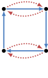
(a)

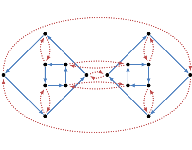
(b)

Figure 4.1: (a) A graph with one bisimulation class and two non-trivial automorphism classes (obtained from reflection on the two diagonals). (b) A graph with one bisimulation class and just one non-trivial automorphism class (obtained from vertical reflection); all vertices participate in single-coloured cycles of the same type.

One could hope that the bisimulation and isomorphism relations for coloured graphs were identical, for then the choice of vertex from a selected $\,\rho_{G}\,$-class would not matter, giving a worst-case $O(\lvert V_{{G}}\rvert\cdot\log\lvert V_{{G}}\rvert)$ canonical labelling algorithm. But, unsurprisingly, this is not the case. Figure 4.1a shows a graph which has a single bisimulation equivalence class but two automorphism equivalence classes. Hence graphs of this kind, where all vertices have the same “local view”, capture the difficult instances of the graph isomorphism and canonical labelling problem for site graphs. The difficulty is essentially that isomorphisms are bijective functions and hence must account for vertex identity at some level. This is not the case for bisimulation equivalence.

One possible solution could be to annotate vertices with additional, “semi-local” information such as edge enumeration up to a constant length, as also suggested in [9], and then take this into account during partition refinement. However, this is unlikely to improve the asymptotic running time. Another approach could be to analyse the cycles of the input graph after partition refinement, and then take this analysis into account during a second partition refinement run on the quotient graph from the first run. The observation here is that all same-coloured paths in the quotient graph are cycles, and these cycles can be detected in linear time. However, vertices with the same local view and single-coloured cycles are not necessarily isomorphic, as demonstrated by Figure 4.1b. It seems that simple cycles of arbitrary colour combinations must be taken into account, e.g. to obtain cycle bases of the graph, but there is no clear means of doing so in linear time. Further attempts in this direction have been unsuccessful.

However, we observe that there are classes of coloured graphs for which bisimulation and isomorphism do coincide. This holds for example for coloured graphs with out and in-degree at most $1$, and more generally for acyclic coloured graphs (trees). For these classes, the partition refinement approach does yield an $O(\lvert V_{{G}}\rvert\cdot\log\lvert V_{{G}}\rvert)$ worst case canonical labelling algorithm. Furthermore, linear time may be possible for these classes using e.g. the partition refinement in [4], assuming an extension similar to that of Algorithm 4 can be realised.

Finally, we note that there is an open question of how the parallel edge enumeration algorithm behaves on graphs with “few” bisimulations. We conjecture that the algorithm may in these cases run in $O(\lvert V_{{G}}\rvert\cdot\log\lvert V_{{G}}\rvert)$ time. If so, partition refinement would be unnecessary. However, for the time being, the partition refinement approach does serve the purpose of providing the upper bound of $O(\lvert V_{{G}}\rvert\cdot\log\lvert V_{{G}}\rvert)$ for graphs with few bisimulations.

5 Conclusions

We have considered the problem of canonical labelling of site graphs, which we have shown reduces to canonical labelling of standard digraphs with edge colourings. We have presented an algorithm based on edge enumeration which runs in $O(\lvert V_{{G}}\rvert^{2})$ worst-case time, and in $O(\lvert V_{{G}}\rvert\cdot\log\lvert V_{{G}}\rvert)$ average-case time for graphs with many automorphisms. A variant of this algorithm, based on parallel enumeration of edges, is likely to perform well in praxis, but in general does not improve on the worst case complexity bounds. However, the question of how the parallel algorithm performs in cases with few automorphisms remains open. If it is found to run in $O(\lvert V_{{G}}\rvert\cdot\log\lvert V_{{G}}\rvert)$ time, this yields an overall $O(\lvert V_{{G}}\rvert\cdot\log\lvert V_{{G}}\rvert)$ average-case algorithm and hence resolves the open question of whether such an algorithm exists. We have also introduced an algorithm based on partition refinement which can be used as a preprocessing step, yielding $O(\lvert V_{{G}}\rvert\cdot\log\lvert V_{{G}}\rvert)$ worst case time for graphs with few bisimulation equivalences.

A different line of attack is taken in [9] which introduces a notion of a graph’s “gravity centre”, namely a subgraph on which it is sufficient to detect automorphisms. Hence this approach is efficient when the gravity centre is small, and could also be a useful pre-processing step for canonical labelling. However, many of the difficult graphs that we have considered, including the one in Figure 4.1b, do not appear to have small gravity centres.

Other related work includes that on the general graph isomorphism problem which has been extensively studied in the literature. Hence highly optimised algorithms, such as the one by McKay [8], exist, although none run in sub-exponential time on “difficult” graphs. Many other special cases have been studied, including notably graphs with bounded degree for which worst-case polynomial time algorithms do exist [1]. Site graphs can indeed be encoded into standard graphs with bounded degree. However, polynomial time algorithms on such encodings do not appear to be sub-quadratic or even quadratic. Perhaps surprisingly, isomorphism of site graphs, or equivalently digraphs with edge colourings, has to the best of our knowledge not been treated in the general literature. Although the difficult cases are perhaps rare and of limited practical relevance, the question is theoretically interesting. It certainly appears to be conducive to infection with the graph isomorphism disease [10].

Acknowledgements

We thank the anonymous reviewers for useful comments. The work of the second author was supported by an EPSRC Postdoctoral Fellowship (EP/H027955/1).

Appendix A Site Graphs and Hopcroft’s Original Algorithm

In the literature site graphs are typically defined as expressions in a language, which is natural when considering simulation and analysis of rule-based models. We give a more direct definition suitable for our purposes. Site graphs in the literature often include internal states of sites, representing e.g. post-translational modification. We omit internal states but they are straightforward to encode.

Definition 16.

Let $(\Sigma_{\text{p}},{\,\preceq_{\text{p}}\,})$ and $(\Sigma_{\text{s}},{\,\preceq_{\text{s}}\,}$) be given, disjoint linearly ordered sets of protein and site names, respectively. Then $\mathcal{SG}$ is the set of all site graphs $S=(V,E,{\phi_{\text{p}}})$ satisfying:

• $V=\{1,\dots,k\}$ is a set of vertices.

• $E\subseteq\binom{V\times\Sigma_{\text{s}}}{2}$ is a set of site-labelled, undirected edges satisfying that $\forall e,e^{\prime}\in E.\,e\neq e^{\prime}\rightarrow e\cap e^{\prime}=\emptyset$.

• ${\phi_{\text{p}}}:V\rightarrow\Sigma_{\text{p}}$ is a vertex (protein) naming.

Note the key condition on edges that a given site can occur at most once within a vertex.

Definition 17.

Let $S,S^{\prime}\in\mathcal{SG}$. A site graph isomorphism is a bijective function $\sigma:V_{{S}}\rightarrow V_{{S^{\prime}}}$ satisfying:

1. $\forall v_{1},v_{2}\in V_{{S}}.\,[\{(v_{1},s_{1}),(v_{2},s_{2})\}\in E_{{S}}\Leftrightarrow\{(\sigma(v_{1}),s_{1}),(\sigma(v_{2}),s_{2})\}\in E_{{S^{\prime}}}]$.

2. $\forall v\in V_{{S}}.\,{\phi_{\text{p}}}_{S}(v)={\phi_{\text{p}}}_{S^{\prime}}(\sigma(v))$.

The first condition states that edges and edge site names are preserved by the isomorphism, and the second condition states that protein names are preserved. We next show how to encode site graphs into coloured graphs. Let $(\Sigma_{\text{p}},{\,\preceq_{\text{p}}\,})$ and $(\Sigma_{\text{s}},{\,\preceq_{\text{s}}\,})$ be given. The aim is to construct a linearly ordered edge colour set $(\Sigma,\prec)$ and a total function $\rho:\mathcal{SG}(\Sigma_{\text{p}},\Sigma_{\text{s}})\rightarrow\mathcal{CG}(\Sigma)$ which preserves isomorphism. We define the colour set as $\Sigma\leavevmode\nobreak\ \overset{\Delta}{\simeq}\leavevmode\nobreak\ \mathcal{{P}}(\Sigma_{\text{s}}\times\Sigma_{\text{s}})\cup\Sigma_{\text{p}}$, and the linear order on $\Sigma$ as $c\prec c^{\prime}$ iff one of the following conditions hold:

• $c\in\Sigma_{\text{p}}\land c^{\prime}\not\in\Sigma_{\text{p}}$  or

• $c,c^{\prime}\in\Sigma_{\text{p}}\land c{\,\preceq_{\text{p}}\,}c^{\prime}$  or

• $c,c^{\prime}\in\mathcal{{P}}(\Sigma_{\text{s}}\times\Sigma_{\text{s}})\land\text{{Sort}}_{{\,\preceq_{\text{s}}\,}}(c){\,\preceq_{\text{s}}\,}\text{{Sort}}_{{\,\preceq_{\text{s}}\,}}c^{\prime}$

In the latter case we assume the ${\,\preceq_{\text{s}}\,}$ relation extended lexicographically to pairs and lists as usual. Let $S\leavevmode\nobreak\ \overset{\Delta}{\simeq}\leavevmode\nobreak\ (V,E,{\phi_{\text{p}}})$ be a given site graph. We then define $\rho(S)\leavevmode\nobreak\ \overset{\Delta}{\simeq}\leavevmode\nobreak\ (V^{\prime},E^{\prime},\phi^{\prime})$ where:

1. $V^{\prime}\leavevmode\nobreak\ \overset{\Delta}{\simeq}\leavevmode\nobreak\ V$.

2. $E^{\prime}\leavevmode\nobreak\ \overset{\Delta}{\simeq}\leavevmode\nobreak\ E^{\prime}_{1}\cup E^{\prime}_{2}$ where:

   1. $E^{\prime}_{1}\leavevmode\nobreak\ \overset{\Delta}{\simeq}\leavevmode\nobreak\ \{(v,v^{\prime})\mid\exists s,s^{\prime}.\,s{\,\preceq_{\text{s}}\,}s^{\prime}\land(s,s^{\prime})=\min_{{\,\preceq_{\text{s}}\,}}\{(s,s^{\prime})\mid\{(v,s),(v^{\prime},s^{\prime})\}\in E\}$

   2. $E^{\prime}_{2}\leavevmode\nobreak\ \overset{\Delta}{\simeq}\leavevmode\nobreak\ \{(v,v)\mid v\in V\}$

3. $\phi^{\prime}(v,v^{\prime})\leavevmode\nobreak\ \overset{\Delta}{\simeq}\leavevmode\nobreak\ C_{1}^{\prime}\cup C_{2}^{\prime}$ where

   1. $C_{1}^{\prime}\leavevmode\nobreak\ \overset{\Delta}{\simeq}\leavevmode\nobreak\ \{(s,s^{\prime})\mid\{(v,s),(v^{\prime},s^{\prime})\}\in E\}$

   2. $C_{2}^{\prime}\leavevmode\nobreak\ \overset{\Delta}{\simeq}\leavevmode\nobreak\ \begin{cases}\{{\phi_{\text{p}}}(v)\}&\,\,\text{{if}}\,\,v=v^{\prime}\\ \emptyset&\,\,\text{{otherwise}}\end{cases}$

The encoding does not affect vertices. Note that site graphs can have multiple unordered edges between nodes while coloured graphs have at most one, ordered edge. The direction of this one edge is determined in Step $2a$ from the site ordering of the least pair of sites, where the least pair of sites is determined from the extension of the site ordering to pairs. All vertices have self-loops (step $2b$) which are used to encode vertex colour as edge colour in step $3b$. Step $3$a assigns a colour to an edge as the union colours of each edge between the edge in the site graph; the ordering of colours follows that assigned to the edge.

Proposition 18.

The coding function $\rho$ satisfies the following for all $S,S^{\prime}\in\operatorname{Dom}(\rho)$:

1. Injective: $\rho(S)=\rho(S^{\prime})\Rightarrow S=S^{\prime}$.

2. Respects isomorphism: $S\simeq S^{\prime}\Leftrightarrow\rho(S)\simeq\rho(S^{\prime})$.

3. Linear size: $\lvert\rho(S)\rvert=O(\lvert S\rvert)$.

4. Linear time computable: $\rho$ is computable in $O(\lvert S\rvert)$.

It follows immediately that the coding function together with a canonical labeller for coloured graphs can be used to define a canonical labeller for site graphs as follows.

Corollary 19.

Given a canonical labeller $L:\prod G\in\mathcal{CG}.\,[G]_{\simeq}$ on coloured graphs running in $O(f(\lvert G\rvert))\geq O(\lvert G\rvert)$ time, the function $L^{*}(S)\leavevmode\nobreak\ \overset{\Delta}{\simeq}\leavevmode\nobreak\ \rho^{-1}(L(\rho(S)))$ is an $O(f(\lvert G\rvert))$ time canonical labeller on site graphs.

input : a graph $G$

output : the relation $\,\rho_{G}\,$

1 $A_{{G}}/\theta\leftarrow\{V_{{G}},V^{\textbf{u}}_{{G}}\}$

2 $L\leftarrow\emptyset$

3 foreach $x\in\Sigma_{{G}}$ do

4       add $(V^{\textbf{u}}_{{G}},x)$ to $L$

5while $L\neq\emptyset$ do

6       remove a pair $(Q,x)$ from $L$

7       foreach $P\in\text{obj}(Q,x,\theta)$ do

8             replace $P$ with $P_{Q,x}$ and $P^{Q,x}$ in $A_{{G}}/\theta$

9            

10      foreach $P$ just refined do

11             foreach $x^{\prime}\in\Sigma_{{G}}$ do

12                   if  $(P,x^{\prime})\in L$ then

13                         replace $(P,x^{\prime})$ with $(P_{Q,x},x^{\prime})$ and $(P^{Q,x},x^{\prime})$ in $L$

14                        

15                  else

16                         AddBetter($(P_{Q,x},x^{\prime})$, $(P^{Q,x},x^{\prime}),x^{\prime},L)$

17                  

18            

19      

20return $\theta$

21 AddBetter($P$,$Q$,$x$,$L$):

22 if $\lvert P\rvert<\lvert Q\rvert$ then

23       add $(P,x)$ to beginning of $L$

24      

25else

26       add $(Q,x)$ to beginning of $L$

27      

Algorithm 5 A version of Hopcroft’s original algorithm adapted from Algorithm $4$ in [6].

References

- Babai and Luks [1983] László Babai and Eugene M. Luks. Canonical labeling of graphs. In Proceedings of the fifteenth annual ACM symposium on Theory of computing, STOC ’83, pages 171–183, New York, NY, USA, 1983. ACM. 10.1145/800061.808746.
- Cardon and Crochemore [1982] A. Cardon and Maxime Crochemore. Partitioning a graph in O(|a| log2 |v|). Theor. Comput. Sci., 19:85–98, 1982. 10.1016/0304-3975(82)90016-0.
- Danos et al. [2007] Vincent Danos, Jérôme Feret, Walter Fontana, and Jean Krivine. Scalable simulation of cellular signaling networks. In APLAS, volume 4807 of LNCS, pages 139–157. Springer, 2007. 10.1007/978-3-540-76637-7_10.
- Dovier et al. [2004] Agostino Dovier, Carla Piazza, and Alberto Policriti. An efficient algorithm for computing bisimulation equivalence. Theor. Comput. Sci, 311:221–256, 2004. 10.1016/S0304-3975(03)00361-X.
- Hopcroft [1971] John E. Hopcroft. An n log n algorithm for minimizing states in a finite automaton. Technical report, Stanford, CA, USA, 1971.
- Knuutila [2001] Timo Knuutila. Re-describing an algorithm by hopcroft. Theor. Comput. Sci., 250(1-2):333–363, January 2001. 10.1016/S0304-3975(99)00150-4.
- Lakin et al. [2012] Matthew R. Lakin, Loïc Paulevé, and Andrew Phillips. Stochastic simulation of multiple process calculi for biology. Theor. Comput. Sci., 431:181–206, 2012. 10.1016/j.tcs.2011.12.057.
- McKay [1981] B. D. McKay. Practical graph isomorphism. Congr. Numer., 30:45–87, 1981.
- Petrov et al. [2012] Tatjana Petrov, Jerome Feret, and Heinz Koeppl. Reconstructing species-based dynamics from reduced stochastic rule-based models. In Proceedings of the Winter Simulation Conference, WSC ’12, pages 1–15. Winter Simulation Conference, 2012. 10.1109/WSC.2012.6465241.
- Read and Cornell [1977] R. C. Read and D. G. Cornell. The graph isomorphism disease. Journal of graph theory, 1(4):339–363, 1977. 10.1002/jgt.3190010410.
- Sipser [1996] Michael Sipser. Introduction to the Theory of Computation. International Thomson Publishing, 1st edition, 1996. ISBN 053494728X. 10.1145/230514.571645.