Flavor Violating Higgs signals in the Texturized Two-Higgs Doublet Model (THDM-Tx)

M. A. Arroyo-Ureña, J. Lorenzo Diaz-Cruz, Enrique Díaz, Javier A. Orduz-Ducuara Facultad de Ciencias Físico-Matemáticas
Benemérita Universidad Autónoma de Puebla, C.P. 72570, Puebla, Pue., Mexico.
Abstract

Flavor violating Higgs signals, such as the top FCNC decay tch0𝑡𝑐superscript0t\to ch^{0} and the LFV Higgs decay h0τμsuperscript0𝜏𝜇h^{0}\to\tau\mu, have been studied at the LHC. These signals can arise within the general Two-Higgs doublet model (THDM), where each Higgs doublet couples to all fermions types through Yukawa matrices Y1fsubscriptsuperscript𝑌𝑓1Y^{f}_{1} and Y2fsubscriptsuperscript𝑌𝑓2Y^{f}_{2}. The Yukawa matrices can be assumed to have the same form or they could have different structures. In this paper we study the case when both Y1fsubscriptsuperscript𝑌𝑓1Y^{f}_{1} and Y2fsubscriptsuperscript𝑌𝑓2Y^{f}_{2} have completely different forms, but in such a way that they complement to produce a specific hermitian mass matrix. We find that for specific four-zero textures, the Flavor Violating Higgs couplings depend only on the free parameters tanβ𝛽\tan\beta, γfsubscript𝛾𝑓\gamma_{f} and the fermion masses. We use the current bounds on the low energy processes, to derive constraints on the Heavy Higgs boson mass, tanβ𝛽\tan\beta and γfsubscript𝛾𝑓\gamma_{f}. Then, we use these constraints to evaluate the LFV Higgs decays, which reach Branching ratios that could be tested at the LHC.

pacs:
Valid PACS appear here
preprint: HEP-BUAP-01.13

I Introduction

The discovery at the Large Hadron Collider (LHC) of a new particle with Standard Model (SM)-Higgs like properties, and mass Mh=125.09±0.21(stat.)±0.11(syst.)M_{h}=125.09\pm 0.21(stat.)\pm 0.11(syst.) GeV [1], seems to confirm the linear realization of the mechanism of Electroweak symmetry breaking. This is needed in order to induce the masses of gauge bosons and fermions within the SM [2]. Furthermore, the current experimental studies at LHC are testing the Higgs properties at levels that could allow to discriminate between the minimal SM Higgs doublet and other extensions of the SM that include more complicated Higgs sectors [3].

In our approach we consider a possible link between the Higgs sector and flavor physics that could be revealed by a thorough study of the THDM with textures (THDM-Tx). In any case such models have a rich phenomenology, with lots of interesting signals that could be searched at future colliders. One of the simplest proposals for physics Beyond the Standard Model, is the so called Two-Higgs Doublet Model (THDM), which was initially studied in connection with the search for the origin of CP violation [4], and later it was used in connection with other theoretical ideas in particle physics, such as supersymmetry [5], extra dimensions [6] and strongly interacting systems [7], [8].

Several possible realizations of the general THDM have been considered in the literature, which have come to be known as Type I, II and III. There are also other models called X, Y, Z, but in some sense they can be considered variations of the above models (for a review see [9]). Model I can have an exact discrete symmetry Z2subscript𝑍2Z_{2}, which permits a possible dark matter candidate coming from the Z2limit-fromsubscript𝑍2Z_{2}-odd scalar doublet [10]. Within type I models, a single Higgs doublet gives mass to the up, down quarks and leptons. The type II model [11] assigns one doublet to each fermion type, then according to the Glashow-Weinberg Theorem [12], this suffices to avoid Flavor Changing Neutral Currents (FCNC) mediated by the Higgs bosons; this type II model also arises in the minimal SUSY extension of the SM [13].

In the most general version of the THDM both Higgs doublets couple to all types of fermions. In this case, the diagonalization of the full mass matrix, does not imply that each Yukawa matrix is diagonalized, therefore FCNC can appear at tree level. Within this general model, one must reproduce the observed fermion masses and mixing angles, while at the same time the level of FCNC must satisfy current experimental bounds [14, 15, 16]. One possibility to achieve this, is the assumption that the Yukawa matrices have a certain texture form, i.e. with zeroes in different elements.

The general model has been previously referred to as the THDM of type III. However, this naming scheme has become confusing, in part because it has also been used to denote a different type of model [17], but also because some specific cases have acquired a relevance of their own. Among the relevant sub-cases of the general THDM, one can include the so-called Minimal Flavor Violating (MFV) THDM [18], which is thought to provide precisely the minimal level of FCNC consistent with data. MFV models could be studied from a pure phenomenological point of view [19], or as arising from flavor symmetries [20]. Although the so-called THDM with Alignment does not contain flavor violation, it is another possibility one can use to obtain realistic models [21]. Thus, in order to clarify the notation and to single out the use of textures within the THDM, from now on we shall call the two-Higgs doublet model with textures as THDM-Tx.

One of the first studies of the THDM with textures [22] considered a specific form with six-zeroes, as well as other variations with cyclic textures. In that work it was identified that the texture assumption implies a specific pattern of FCNC Higgs-fermion couplings, known nowadays as the Cheng-Sher ansatz, which is of size mimjvsubscript𝑚𝑖subscript𝑚𝑗𝑣\frac{\sqrt{m_{i}m_{j}}}{v}. It was found that such vertex could satisfy FCNC bounds with Higgs masses lighter than O(TeV). The extension of the THDM-Tx with a four-zero texture was presented in [23, 24]. The phenomenological consequences of these textures (Hermitian 4-textures or non-hermitian 6-textures) were considered in [25], while further phenomenological studies were presented in [26, 27, 28].

Several models for Yukawa matrices could be identified which lead to specific patterns of flavor violating Higgs interactions. For instance, one can assume that the Yukawa matrices Y1fsubscriptsuperscript𝑌𝑓1Y^{f}_{1} and Y2fsubscriptsuperscript𝑌𝑓2Y^{f}_{2} have the same form (a case that we call “Parallel Textures”). It is also possible to have a Yukawa matrix, say Y1fsubscriptsuperscript𝑌𝑓1Y^{f}_{1}, with some specific texture, while the second matrix Y2fsubscriptsuperscript𝑌𝑓2Y^{f}_{2} has only some elements different from zero, at positions that coincide with some elements of Y1fsubscriptsuperscript𝑌𝑓1Y^{f}_{1}, as in the so called top-specific models discussed in the literature [29], we call this case “Semi-parallel textures”.

In this paper we study another possibility, namely that Y1fsubscriptsuperscript𝑌𝑓1Y^{f}_{1} and Y2fsubscriptsuperscript𝑌𝑓2Y^{f}_{2} have completely different structure. Namely, for specific four-zero textures that reproduce all fermion masses and the CKM matrix, these vertices only depend on the parameters tanβ(=v2v1)annotated𝛽absentsubscript𝑣2subscript𝑣1\tan\beta(=\frac{v_{2}}{v_{1}}) and γfsubscript𝛾𝑓\gamma_{f} (0<γf<1,f=u,d,l)formulae-sequence0subscript𝛾𝑓1𝑓𝑢𝑑𝑙(0<\gamma_{f}<1,f=u,d,l), which appears in the relation between the third family mass and the 33 entry of the corresponding mass matrix. We use the current bounds on the low energy processes, to impose constraints on the values of γfsubscript𝛾𝑓\gamma_{f} and tanβ𝛽\tan\beta. We also compare these constraints with the ones obtained for the cases of parallel and fermion-specific textures. Furthermore, we also include the constraints obtained from current LHC bounds on the Higgs boson couplings, and derive predictions for the Flavor Violating decays h0τμsuperscript0𝜏𝜇h^{0}\to\tau\mu and tch0𝑡𝑐superscript0t\to ch^{0}, which reach Branching ratios that could be tested at the LHC in the forthcoming era of precision Flavor Higgs Physics.

The organization of our paper is as follows. A classification of the different types of Yukawa matrices that produce a mass matrix with four-zero textures, as well as the diagonalization of the mass matrix, is presented in section II. Section III discusses generalities of the THDM-Tx, including the Yukawa interaction Lagrangian written in terms of mass eigenstates. Low energy constraints are discussed in section IV, including KK¯𝐾¯𝐾K-\bar{K} and BB¯𝐵¯𝐵B-\bar{B} mixing, Bs0μ+μsuperscriptsubscript𝐵𝑠0superscript𝜇superscript𝜇B_{s}^{0}\to\mu^{+}\mu^{-}, μeγ𝜇𝑒𝛾\mu\rightarrow e\gamma, τμμ+μsuperscript𝜏superscript𝜇superscript𝜇superscript𝜇\tau^{-}\rightarrow\mu^{-}\mu^{+}\mu^{-}, BD(D)τν𝐵𝐷superscript𝐷𝜏𝜈B\to D(D^{*})\tau\nu and ΔaμΔsubscript𝑎𝜇\Delta a_{\mu}. Constraints from current Higgs searches at LHC are included in section V. The prediction of our model for the decays h0τμsuperscript0𝜏𝜇h^{0}\to\tau\mu and tch0,𝑡𝑐superscript0t\to ch^{0}, are discussed in section VI. Conclusions of our work are presented in section VII,

II Fermion Mass Matrix: Diagonalization and Texture Patterns

Within the general THDM, each Higgs doublet couples to fermions of type f𝑓f (f=u,d,l𝑓𝑢𝑑𝑙f=u,d,l) through the Yukawa matrices Y1fsubscriptsuperscript𝑌𝑓1Y^{f}_{1} and Y2fsubscriptsuperscript𝑌𝑓2Y^{f}_{2}. After Spontaneous Symmetry Breaking (SSB), these matrices combine to produce a fermion mass matrix with some structure. The mass matrix for each fermion type f(=u,d,l)f(=u,d,l) receives contributions from both vevs v1subscript𝑣1v_{1} and v2subscript𝑣2v_{2}, i.e.

Mf=12(v1Y1f+v2Y2f),subscript𝑀𝑓12subscript𝑣1subscriptsuperscript𝑌𝑓1subscript𝑣2subscriptsuperscript𝑌𝑓2{M_{f}}=\frac{1}{\sqrt{2}}\left(v_{1}{Y}^{f}_{1}+v_{2}{Y}^{f}_{2}\right), (1)

To obtain physical fermion masses we need to diagonalize the mass matrix; this is achieved through a bi-unitary transformation 𝒪f=VfPfsubscript𝒪𝑓superscriptsubscript𝑉𝑓subscript𝑃𝑓\mathcal{O}_{f}=V_{f}^{\dagger}P_{f}, i.e.

MD=𝒪fMf𝒪f=𝒪f12(v1Y1f+v2Y2f)𝒪f,subscript𝑀𝐷subscript𝒪𝑓subscript𝑀𝑓superscriptsubscript𝒪𝑓subscript𝒪𝑓12subscript𝑣1subscriptsuperscript𝑌𝑓1subscript𝑣2subscriptsuperscript𝑌𝑓2superscriptsubscript𝒪𝑓{M_{D}}=\mathcal{O}_{f}{M_{f}}\mathcal{O}_{f}^{\dagger}=\mathcal{O}_{f}\frac{1}{\sqrt{2}}\left(v_{1}{Y}^{f}_{1}+v_{2}{Y}^{f}_{2}\right)\mathcal{O}_{f}^{\dagger}, (2)

the form of the matrix 𝒪fsubscript𝒪𝑓\mathcal{O}_{f} depends on the texture type; closed forms have been obtained for the 4- and 6-texture hermitian and non-hermitian cases. Although 𝒪fsubscript𝒪𝑓\mathcal{O}_{f} diagonalizes the matrix Mfsubscript𝑀𝑓M_{f}, it does not necessarily diagonalize each of the Yukawa matrices that make up Mfsubscript𝑀𝑓M_{f}, thus neutral flavor violating Higgs-fermion interactions will be induced.

II.1 Diagonalization of the Fermion mass matrices of four-texture type

For the 4-texture case the mass matrix takes the form:

Mf=(0D0DCB0BA),subscript𝑀𝑓0𝐷0superscript𝐷𝐶𝐵0superscript𝐵𝐴\displaystyle{M_{f}}=\left(\begin{array}[]{ccc}0&D&0\\ D^{*}&C&B\\ 0&B^{*}&A\end{array}\right), (6)

then 𝒪fsubscript𝒪𝑓\mathcal{O}_{f} is given by:

𝒪f=(m2m3(Am1)A(m2m1)(m3m1)m1m3(m2A)A(m2m1)(m3m2)m1m2(Am3)A(m3m1)(m3m2)m1(m1A)(m2m1)(m3m1)m2(Am2)(m2m1)(m3m2)m3(m3A)(m3m1)(m3m2)m1(Am2)(Am3)A(m2m1)(m3m1)m2(Am1)(m3A)A(m2m1)(m3m2)m3(Am1)(Am2)A(m3m1)(m3m2)),subscript𝒪𝑓subscript𝑚2subscript𝑚3𝐴subscript𝑚1𝐴subscript𝑚2subscript𝑚1subscript𝑚3subscript𝑚1subscript𝑚1subscript𝑚3subscript𝑚2𝐴𝐴𝑚2subscript𝑚1subscript𝑚3subscript𝑚2subscript𝑚1subscript𝑚2𝐴subscript𝑚3𝐴subscript𝑚3subscript𝑚1subscript𝑚3subscript𝑚2subscript𝑚1subscript𝑚1𝐴subscript𝑚2subscript𝑚1subscript𝑚3subscript𝑚1subscript𝑚2𝐴subscript𝑚2subscript𝑚2subscript𝑚1subscript𝑚3subscript𝑚2subscript𝑚3subscript𝑚3𝐴subscript𝑚3subscript𝑚1subscript𝑚3subscript𝑚2subscript𝑚1𝐴subscript𝑚2𝐴subscript𝑚3𝐴subscript𝑚2subscript𝑚1subscript𝑚3subscript𝑚1subscript𝑚2𝐴subscript𝑚1subscript𝑚3𝐴𝐴subscript𝑚2subscript𝑚1subscript𝑚3subscript𝑚2subscript𝑚3𝐴subscript𝑚1𝐴subscript𝑚2𝐴subscript𝑚3subscript𝑚1subscript𝑚3subscript𝑚2\displaystyle\small\mathcal{O}_{f}=\left(\begin{array}[]{ccc}\sqrt{\frac{m_{2}m_{3}(A-m_{1})}{A(m_{2}-m_{1})(m_{3}-m_{1})}}&\sqrt{\frac{m_{1}m_{3}(m_{2}-A)}{A(m2-m_{1})(m_{3}-m_{2})}}&\sqrt{\frac{m_{1}m_{2}(A-m_{3})}{A(m_{3}-m_{1})(m_{3}-m_{2})}}\\ -\sqrt{\frac{m_{1}(m_{1}-A)}{(m_{2}-m_{1})(m_{3}-m_{1})}}&\sqrt{\frac{m_{2}(A-m_{2})}{(m_{2}-m_{1})(m_{3}-m_{2})}}&\sqrt{\frac{m_{3}(m_{3}-A)}{(m_{3}-m_{1})(m_{3}-m_{2})}}\\ \sqrt{\frac{m_{1}(A-m_{2})(A-m_{3})}{A(m_{2}-m_{1})(m_{3}-m_{1})}}&-\sqrt{\frac{m_{2}(A-m_{1})(m_{3}-A)}{A(m_{2}-m_{1})(m_{3}-m_{2})}}&\sqrt{\frac{m_{3}(A-m_{1})(A-m_{2})}{A(m_{3}-m_{1})(m_{3}-m_{2})}}\end{array}\right), (10)

and

Pf=(1000eiα1000eiα2).subscript𝑃𝑓1000superscript𝑒𝑖subscript𝛼1000superscript𝑒𝑖subscript𝛼2\displaystyle P_{f}=\left(\begin{array}[]{ccc}1&0&0\\ 0&e^{i\alpha_{1}}&0\\ 0&0&e^{i\alpha_{2}}\\ \end{array}\right). (14)

where misubscript𝑚𝑖m_{i} (i=1,2,3)𝑖123(i=1,2,3) are the fermion masses. Hence, following refs. [14, 15], we use det(Mf)=D2A=m1m2m3𝑑𝑒𝑡subscript𝑀𝑓superscript𝐷2𝐴subscript𝑚1subscript𝑚2subscript𝑚3det(M_{f})=-D^{2}A=m_{{1}}m_{{2}}m_{{3}} and assume the ordering m3>A>m2>m1subscript𝑚3𝐴subscript𝑚2subscript𝑚1m_{{3}}>A>m_{{2}}>m_{{1}}, so that Am3<0𝐴subscript𝑚30A-m_{{3}}<0, to get real mixing angles we take m1<0subscript𝑚10m_{{1}}<0.

From these expressions we find a relation between the components of the 4-texture mass matrix and the physical fermion masses, which will be useful in order to find the expressions for the Higgs-fermion interactions, namely:

A𝐴\displaystyle A =\displaystyle= m3(1r2γf),subscript𝑚31subscript𝑟2subscript𝛾𝑓\displaystyle m_{{3}}\left(1-r_{2}\gamma_{f}\right), (15)
B𝐵\displaystyle B =\displaystyle= m3r2γf(r2γf+r11)(r2γf+r21)1r2γf,subscript𝑚3subscript𝑟2subscript𝛾𝑓subscript𝑟2subscript𝛾𝑓subscript𝑟11subscript𝑟2subscript𝛾𝑓subscript𝑟211subscript𝑟2subscript𝛾𝑓\displaystyle m_{{3}}\sqrt{\frac{r_{{2}}\gamma_{f}\left(r_{{2}}\gamma_{f}+r_{{1}}-1\right)\left(r_{{2}}\gamma_{f}+r_{{2}}-1\right)}{1-r_{{2}}\gamma_{f}}}, (16)
C𝐶\displaystyle C =\displaystyle= m3(r2γf+r1+r2),subscript𝑚3subscript𝑟2subscript𝛾𝑓subscript𝑟1subscript𝑟2\displaystyle m_{{3}}\left(r_{2}\gamma_{f}+r_{{1}}+r_{{2}}\right), (17)
D𝐷\displaystyle D =\displaystyle= m1m21r2γf,\displaystyle\sqrt{-\frac{m_{{1}}m_{{2}}}{1-r_{{2}}\gamma_{f}},} (18)

where ri=mim3.subscript𝑟𝑖subscript𝑚𝑖subscript𝑚3r_{{i}}=\frac{m_{{i}}}{m_{{3}}}. Thus, the relation between the third family mass and the 33 entry of the mass matrix A=m3(1r2γf)𝐴subscript𝑚31subscript𝑟2subscript𝛾𝑓A=m_{{3}}(1-r_{{2}}\gamma_{f}), depends on the parameter γfsubscript𝛾𝑓\gamma_{f} (0<γf<10subscript𝛾𝑓10<\gamma_{f}<1), where f=u,d,l𝑓𝑢𝑑𝑙f=u,d,l. Concerning the construction of the physical CKM matrix VCKM=𝒪u𝒪dsubscript𝑉𝐶𝐾𝑀subscript𝒪𝑢superscriptsubscript𝒪𝑑V_{CKM}=\mathcal{O}_{u}\mathcal{O}_{d}^{\dagger}, we are able to correctly reproduce the values of CKM matrix [30]; for example for the values of γu=0.13subscript𝛾𝑢0.13\gamma_{u}=0.13, γd=0.1subscript𝛾𝑑0.1\gamma_{d}=0.1, α1u=2.473555superscriptsubscript𝛼1𝑢2.473555\alpha_{1}^{u}=2.473555, α2u=0.65superscriptsubscript𝛼2𝑢0.65\alpha_{2}^{u}=0.65, α1d=1.045superscriptsubscript𝛼1𝑑1.045\alpha_{1}^{d}=1.045 and α2d=1.69superscriptsubscript𝛼2𝑑1.69\alpha_{2}^{d}=1.69, we obtain

VCKMTHDMTx=(0.974240.225480.002940.225300.973420.041000.009180.040000.99915).superscriptsubscript𝑉𝐶𝐾𝑀𝑇𝐻𝐷𝑀𝑇𝑥0.974240.225480.002940.225300.973420.041000.009180.040000.99915\displaystyle{V}_{CKM}^{THDM-Tx}=\left(\begin{array}[]{ccc}0.97424&0.22548&0.00294\\ 0.22530&0.97342&0.04100\\ 0.00918&0.04000&0.99915\end{array}\right). (22)

II.2 Classification of Textures: Parallel, Semi-Parallel and Complementary

For the purpose of studying the fermion masses and CKM mixing matrix, it does not matter how each Yukawa matrix contributes to the mass matrix. These matrices can be obtained from a variety of flavor symmetries, discrete or continuos, local or global, in 4D or beyond. It could be interesting to look for some experimental signals that could help to discriminate among all those different possibilities. It turns out that the flavor violating Higgs interactions could provide such methodology.

Rather than focusing on an specific model, we study here the different possibilities one could use in order to arrive to some mass matrix Mfsubscript𝑀𝑓M_{f} from the different patterns of Yukawa matrices Y1fsubscriptsuperscript𝑌𝑓1Y^{f}_{1} and Y2fsubscriptsuperscript𝑌𝑓2Y^{f}_{2}. In such case one can express one rotated Yukawa matrix in terms of the other one and the mass eigenvalues. For instance we can rotate Y1subscript𝑌1Y_{1}, and fix Y2subscript𝑌2Y_{2} through the relation: Y2~=2v2M¯fcotβY~1~subscript𝑌22subscript𝑣2subscript¯𝑀𝑓𝛽subscript~𝑌1\tilde{Y_{2}}=\frac{\sqrt{2}}{v_{2}}\bar{M}_{f}-\cot\beta\tilde{Y}_{1}.

I) “Parallel textures”. This is the most widely studied case, which assumes that both Y1fsubscriptsuperscript𝑌𝑓1{Y}^{f}_{1} and Y2fsubscriptsuperscript𝑌𝑓2{Y}^{f}_{2} have the same structure, namely:

Y1=(0d10d1c1b10b1a1),Y2=(0d20d2c2b20b2a2).formulae-sequencesubscript𝑌1matrix0subscript𝑑10subscriptsuperscript𝑑1subscript𝑐1subscript𝑏10subscriptsuperscript𝑏1subscript𝑎1subscript𝑌2matrix0subscript𝑑20subscriptsuperscript𝑑2subscript𝑐2subscript𝑏20subscriptsuperscript𝑏2subscript𝑎2\displaystyle Y_{1}=\begin{pmatrix}0&d_{1}&0\\ d^{*}_{1}&c_{1}&b_{1}\\ 0&b^{*}_{1}&a_{1}\\ \end{pmatrix},\hskip 14.22636ptY_{2}=\begin{pmatrix}0&d_{2}&0\\ d^{*}_{2}&c_{2}&b_{2}\\ 0&b^{*}_{2}&a_{2}\\ \end{pmatrix}. (23)

The explicit form of the 33 and 23 elements for the rotated Yukawa matrix Y~2fsubscriptsuperscript~𝑌𝑓2\tilde{Y}^{f}_{2} is given by:

(Y~2f)23subscriptsubscriptsuperscript~𝑌𝑓223\displaystyle({\tilde{Y}}^{f}_{2})_{23} =\displaystyle= m2m3vχ23,subscript𝑚2subscript𝑚3𝑣subscript𝜒23\displaystyle\frac{\sqrt{m_{2}m_{3}}}{v}\chi_{23}, (24)
(Y~2f)33subscriptsubscriptsuperscript~𝑌𝑓233\displaystyle({\tilde{Y}}^{f}_{2})_{33} =\displaystyle= m3vχ33,subscript𝑚3𝑣subscript𝜒33\displaystyle\frac{m_{3}}{v}\chi_{33}, (25)

where

χ23=m3m2(b1vm3tanβF1sinβ)eiα2+((a1c1)vm3tanβ2F2sinβ)γf,subscript𝜒23subscript𝑚3subscript𝑚2subscript𝑏1𝑣subscript𝑚3𝛽subscript𝐹1𝛽superscript𝑒𝑖subscript𝛼2subscript𝑎1subscript𝑐1𝑣subscript𝑚3𝛽2subscript𝐹2𝛽subscript𝛾𝑓\chi_{23}=\sqrt{\frac{m_{3}}{m_{2}}}\left(\frac{b_{1}v}{m_{3}\tan\beta}-\frac{F_{1}}{\sin\beta}\right)e^{i\alpha_{2}}+\left(\frac{(a_{1}-c_{1})v}{m_{3}\tan\beta}-\sqrt{2}\frac{F_{2}}{\sin\beta}\right)\sqrt{\gamma_{f}}, (26)
χ33=2F1Q(b1vm3tanβF1sinβ)cosα2c1vm3tanβF3+2(QF3R)sinβ.subscript𝜒332subscript𝐹1𝑄subscript𝑏1𝑣subscript𝑚3𝛽subscript𝐹1𝛽subscript𝛼2subscript𝑐1𝑣subscript𝑚3𝛽subscript𝐹32𝑄subscript𝐹3𝑅𝛽\chi_{33}=\sqrt{2}\frac{F_{1}}{Q}\left(\frac{b_{1}v}{m_{3}\tan\beta}-\frac{F_{1}}{\sin\beta}\right)\cos\alpha_{2}-\frac{c_{1}v}{m_{3}\tan\beta}F_{3}+\sqrt{2}\frac{(Q-F_{3}R)}{\sin\beta}. (27)

We define r2=m2/m3subscript𝑟2subscript𝑚2subscript𝑚3r_{2}=m_{2}/m_{3}, R=1r2γfr2𝑅1subscript𝑟2subscript𝛾𝑓subscript𝑟2R=1-r_{2}\gamma_{f}-r_{2}, Q=1r2𝑄1subscript𝑟2Q=1-r_{2}, G=r2γf𝐺subscript𝑟2subscript𝛾𝑓G=r_{2}\gamma_{f}, F1=2GRsubscript𝐹12𝐺𝑅F_{1}=\sqrt{2GR}, F2=Q2Gsubscript𝐹2𝑄2𝐺F_{2}=Q-2G, F3=G/Qsubscript𝐹3𝐺𝑄F_{3}=G/Q. In this case, the elements χ23,33subscript𝜒2333\chi_{23,33} depend on the complete set of parameters a1subscript𝑎1a_{1}, b1subscript𝑏1b_{1}, c1subscript𝑐1c_{1}, α2subscript𝛼2\alpha_{2}, γfsubscript𝛾𝑓\gamma_{f} and β𝛽\beta. In the literature [25], it is usually assumed that these elements already have the Cheng-Sher form, with coefficients χijfsubscriptsuperscript𝜒𝑓𝑖𝑗\chi^{f}_{ij} of O(1)𝑂1O(1), which are constrained from analyzing the FCNC and LFV processes.

II) “Semi-Parallel textures”. However, it is also possible that Y1fsubscriptsuperscript𝑌𝑓1{Y}^{f}_{1} and Y2fsubscriptsuperscript𝑌𝑓2{Y}^{f}_{2} could have different textures, but in such a way that the resulting mass matrix has a realistic texture. It could be that Y1fsubscriptsuperscript𝑌𝑓1Y^{f}_{1} has a certain texture, but Y2fsubscriptsuperscript𝑌𝑓2Y^{f}_{2} has some entry different from zero in one of the entries that is also non-zero for Y1fsubscriptsuperscript𝑌𝑓1Y^{f}_{1}. One example has Y1fsubscriptsuperscript𝑌𝑓1Y^{f}_{1} with a four-zero texture, while Y2fsubscriptsuperscript𝑌𝑓2{Y}^{f}_{2} has only a non-zero 33 entry, namely:

Y1=(0d10d1c1b10b1a1),Y2=(00000000a2).formulae-sequencesubscript𝑌1matrix0subscript𝑑10subscriptsuperscript𝑑1subscript𝑐1subscript𝑏10subscriptsuperscript𝑏1subscript𝑎1subscript𝑌2matrix00000000subscript𝑎2Y_{1}=\begin{pmatrix}0&d_{1}&0\\ d^{*}_{1}&c_{1}&b_{1}\\ 0&b^{*}_{1}&a_{1}\\ \end{pmatrix},\hskip 14.22636ptY_{2}=\begin{pmatrix}0&0&0\\ 0&0&0\\ 0&0&a_{2}\\ \end{pmatrix}. (28)

These cases could be called Semi-Parallel textures. The explicit form of the 33 and 23 elements is given by:

(Y~2f)23subscriptsubscriptsuperscript~𝑌𝑓223\displaystyle(\tilde{Y}^{f}_{2})_{23} =\displaystyle= m2m3vχ23,subscript𝑚2subscript𝑚3𝑣subscript𝜒23\displaystyle\frac{\sqrt{m_{2}m_{3}}}{v}\chi_{23}, (29)
(Y~2f)33subscriptsubscriptsuperscript~𝑌𝑓233\displaystyle(\tilde{Y}^{f}_{2})_{33} =\displaystyle= m3vχ33,subscript𝑚3𝑣subscript𝜒33\displaystyle\frac{m_{3}}{v}\chi_{33},

where χ23=RQ(2Psinβa1vm3tanβ)γfsubscript𝜒23𝑅𝑄2𝑃𝛽subscript𝑎1𝑣subscript𝑚3𝛽subscript𝛾𝑓\chi_{23}=\frac{\sqrt{R}}{Q}\left(\frac{\sqrt{2}P}{\sin{\beta}}-\frac{a_{1}v}{m_{3}}\tan\beta\right)\sqrt{\gamma_{f}}, χ33=RQ(2Psinβa1vm3tanβ)subscript𝜒33𝑅𝑄2𝑃𝛽subscript𝑎1𝑣subscript𝑚3𝛽\chi_{33}=\frac{R}{Q}\left(\frac{\sqrt{2}P}{\sin{\beta}}-\frac{a_{1}v}{m_{3}}\tan\beta\right) and P=1r2γf𝑃1subscript𝑟2subscript𝛾𝑓P=1-r_{2}\gamma_{f}. In this case the elements depend on the parameters a1subscript𝑎1a_{1}, β𝛽\beta and γfsubscript𝛾𝑓\gamma_{f} which simplifies the study of the phenomenology of the model.

III) “Complementary textures” Here, we consider Yukawa matrices that have a different structure, but in such a way that they produce a hermitian mass matrix with four zero textures. We shall consider patterns where at most one element from each of the Yukawa matrices Y1,2fsubscriptsuperscript𝑌𝑓12{Y}^{f}_{1,2} contributes to one entry of the full mass matrix.

Thus the cases that will be considered are defined as follows:

Y1=(0d0dcb0b0),Y2=(00000000a).formulae-sequencesubscript𝑌1matrix0𝑑0superscript𝑑𝑐𝑏0superscript𝑏0subscript𝑌2matrix00000000𝑎Y_{1}=\begin{pmatrix}0&d&0\\ d^{*}&c&b\\ 0&b^{*}&0\end{pmatrix},\hskip 14.22636ptY_{2}=\begin{pmatrix}0&0&0\\ 0&0&0\\ 0&0&a\end{pmatrix}. (30)

The explicit form of the 33 and 23 elements is given by:

(Y2f~)23=m2m3vχ23,subscript~subscriptsuperscript𝑌𝑓223subscript𝑚2subscript𝑚3𝑣subscript𝜒23(\tilde{Y^{f}_{2}})_{23}=\frac{\sqrt{m_{2}m_{3}}}{v}\chi_{23}, (31)
(Y2f~)33=m3vχ33,subscript~subscriptsuperscript𝑌𝑓233subscript𝑚3𝑣subscript𝜒33(\tilde{Y^{f}_{2}})_{33}=\frac{m_{3}}{v}\chi_{33}, (32)

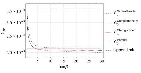
where χ23=RQ2Psinβγfsubscript𝜒23𝑅𝑄2𝑃𝛽subscript𝛾𝑓\chi_{23}=\frac{\sqrt{R}}{Q}\frac{\sqrt{2}P}{\sin\beta}\sqrt{\gamma_{f}} and χ33=RQ2Psinβsubscript𝜒33𝑅𝑄2𝑃𝛽\chi_{33}=\frac{R}{Q}\frac{\sqrt{2}P}{\sin\beta}. We can see that in the limit a10subscript𝑎10a_{1}\to 0 the Semi-Parallel case is reduced to the Complementary case. In this case the elements depend only on the parameters β𝛽\beta and γfsubscript𝛾𝑓\gamma_{f} which is simplest case for the study of the phenomenology of the model because it has only two parameters. In Fig 1 a comparison is made between the Cheng-Sher ansatz and corrections arising from the elements of χijsubscript𝜒𝑖𝑗\chi_{ij} of order 𝒪(1)𝒪1\mathcal{O}(1) [31] which comes from the considered textures.
Refer to caption
Figure 1: Plots of Yτμsubscript𝑌𝜏𝜇Y_{\tau\mu}(=mτmμvχτμabsentsubscript𝑚𝜏subscript𝑚𝜇𝑣subscript𝜒𝜏𝜇=\frac{\sqrt{m_{\tau}m_{\mu}}}{v}\chi_{\tau\mu}) vs tanβ𝛽\tan{\beta}, with χτμsubscript𝜒𝜏𝜇\chi_{\tau\mu}=1 for the Cheng-Sher ansatz and χτμ1similar-tosubscript𝜒𝜏𝜇1\chi_{\tau\mu}\sim 1 for the considered cases, i.e., Parallel, Semi-Parallel and Complementary. The highest line indicates the upper bound of the Yukawa coupling of τ𝜏\tau-μ𝜇\mu.

The example of “Complementary textures” is called case 1, while the characteristics of other possible variations (cases 2-6) are included the appendix A, where some salient features are also mentioned. In making these choices, we have assigned the 33 mass entry to Y2subscript𝑌2Y_{2}. Our convention is motivated by the assumption that the largest Yukawa element is expected to arise from some dominant mechanism (unknown) while the lightest masses and CKM mixing could be the result of some perturbation to the above mechanism. The logic of our ordering is to start from the simplest structure for Y2subscript𝑌2Y_{2}, i.e., with only (Y2)330subscriptsubscript𝑌2330(Y_{2})_{33}\neq 0 (case 1), up to the more complicated case, where Y2subscript𝑌2Y_{2} itself is of the 3-texture type.

III The Higgs Interaction in the THDM-Tx

III.1 The General Yukawa Lagrangian

The Yukawa Lagrangian in the THDM-III is given by [25, 32]

\displaystyle\mathcal{L} =\displaystyle= Y1uQ¯L0Φ~1uR0+Y2uQ¯L0Φ~2uR0+Y1dQ¯L0Φ1dR0+Y2dQ¯L0Φ2dR0subscriptsuperscript𝑌𝑢1superscriptsubscript¯𝑄𝐿0subscript~Φ1superscriptsubscript𝑢𝑅0subscriptsuperscript𝑌𝑢2superscriptsubscript¯𝑄𝐿0subscript~Φ2superscriptsubscript𝑢𝑅0subscriptsuperscript𝑌𝑑1superscriptsubscript¯𝑄𝐿0subscriptΦ1superscriptsubscript𝑑𝑅0subscriptsuperscript𝑌𝑑2superscriptsubscript¯𝑄𝐿0subscriptΦ2superscriptsubscript𝑑𝑅0\displaystyle{Y^{u}_{1}}\overline{Q}_{L}^{0}{\tilde{\Phi}_{1}}u_{R}^{0}+{{{{Y^{u}_{2}}}}}\overline{Q}_{L}^{0}{\tilde{\Phi}_{2}}u_{R}^{0}+{{{{Y^{d}_{1}}}}}\overline{Q}_{L}^{0}{\Phi_{1}}d_{R}^{0}+{Y^{d}_{2}}\overline{Q}_{L}^{0}{\Phi_{2}}d_{R}^{0} (33)
+\displaystyle+ Y1lL¯0Φ1lR0+Y2lL¯0Φ2lR0+h.c.,formulae-sequencesuperscriptsubscript𝑌1𝑙superscript¯𝐿0subscriptΦ1superscriptsubscript𝑙𝑅0superscriptsubscript𝑌2𝑙superscript¯𝐿0subscriptΦ2superscriptsubscript𝑙𝑅0𝑐\displaystyle{{Y_{1}^{l}}}\overline{L}^{0}{\Phi_{1}}l_{R}^{0}+{Y_{2}^{l}}\overline{L}^{0}{\Phi_{2}}l_{R}^{0}+h.c.,

such that

QL0subscriptsuperscript𝑄0𝐿\displaystyle Q^{0}_{L} =\displaystyle= (uLdL),L0=(νLeL),Φ1=(ϕ1+ϕ10),Φ2=(ϕ2+ϕ20),formulae-sequencesubscript𝑢𝐿subscript𝑑𝐿superscript𝐿0subscript𝜈𝐿subscript𝑒𝐿formulae-sequencesubscriptΦ1superscriptsubscriptitalic-ϕ1superscriptsubscriptitalic-ϕ10subscriptΦ2superscriptsubscriptitalic-ϕ2superscriptsubscriptitalic-ϕ20\displaystyle\left(\begin{array}[]{c}u_{L}\\ d_{L}\\ \end{array}\right),\hskip 8.53581ptL^{0}=\left(\begin{array}[]{c}\nu_{L}\\ e_{L}\\ \end{array}\right),\hskip 8.53581pt\Phi_{1}=\left(\begin{array}[]{c}\phi_{1}^{+}\\ \phi_{1}^{0}\\ \end{array}\right),\hskip 8.53581pt\Phi_{2}=\left(\begin{array}[]{c}\phi_{2}^{+}\\ \phi_{2}^{0}\\ \end{array}\right), (42)
Φ~jsubscript~Φ𝑗\displaystyle\tilde{\Phi}_{j} =\displaystyle= iσ2Φj=(ϕj0ϕj).𝑖subscript𝜎2superscriptsubscriptΦ𝑗superscriptsuperscriptsubscriptitalic-ϕ𝑗0superscriptsubscriptitalic-ϕ𝑗\displaystyle i\sigma_{2}\Phi_{j}^{*}=\left(\begin{array}[]{c}{\phi_{j}^{0}}^{*}\\ -\phi_{j}^{-}\\ \end{array}\right). (45)

The physical fields are defined through a transformation that depends on the angle α𝛼\alpha which transforms the real part neutral physical Higgs bosons:

(H0h0)=(cosαsinαsinαcosα)(Reϕ1Reϕ2),superscript𝐻0superscript0𝛼𝛼𝛼𝛼𝑅𝑒subscriptitalic-ϕ1𝑅𝑒subscriptitalic-ϕ2\displaystyle\left(\begin{array}[]{c}H^{0}\\ h^{0}\\ \end{array}\right)=\left(\begin{array}[]{cc}\cos\alpha&\sin\alpha\\ -\sin\alpha&\cos\alpha\\ \end{array}\right)\cdot\left(\begin{array}[]{c}Re\phi_{1}\\ Re\phi_{2}\\ \end{array}\right), (52)

and the angle β𝛽\beta which that transforms the imaginary part neutral and charged physical Higgs bosons given by

(G0A0)=(cosβsinβsinβcosβ)(Imϕ1Imϕ2),superscript𝐺0superscript𝐴0𝛽𝛽𝛽𝛽𝐼𝑚subscriptitalic-ϕ1𝐼𝑚subscriptitalic-ϕ2\displaystyle\left(\begin{array}[]{c}G^{0}\\ A^{0}\\ \end{array}\right)=\left(\begin{array}[]{cc}\cos\beta&\sin\beta\\ -\sin\beta&\cos\beta\\ \end{array}\right)\cdot\left(\begin{array}[]{c}Im\phi_{1}\\ Im\phi_{2}\\ \end{array}\right), (59)
(G±H±)=(cosβsinβsinβcosβ)(ϕ1±ϕ±),superscript𝐺plus-or-minussuperscript𝐻plus-or-minus𝛽𝛽𝛽𝛽superscriptsubscriptitalic-ϕ1plus-or-minussubscriptitalic-ϕplus-or-minus\displaystyle\left(\begin{array}[]{c}G^{\pm}\\ H^{\pm}\\ \end{array}\right)=\left(\begin{array}[]{cc}\cos\beta&\sin\beta\\ -\sin\beta&\cos\beta\\ \end{array}\right)\cdot\left(\begin{array}[]{c}\phi_{1}^{\pm}\\ \phi_{\pm}\\ \end{array}\right), (66)

the angle β𝛽\beta is defined as

tanβ=v2v1.𝛽subscript𝑣2subscript𝑣1\tan\beta=\frac{v_{2}}{v_{1}}. (67)

As a matter of convenience we separate the Lagrangian into charged (chsubscript𝑐\mathcal{L}_{ch}) and neutral sector (nsubscript𝑛\mathcal{L}_{n}). Thus,

nsubscript𝑛\displaystyle\mathcal{L}_{n} =\displaystyle= g2(mdmW)d¯[cosαcosβδdd+2sin(αβ)gcosβ(mWmd)(Y~2d)dd]dH0\displaystyle\frac{g}{2}\left(\frac{m_{d}}{m_{W}}\right)\bar{d}\left[\frac{\cos\alpha}{\cos\beta}\delta_{dd{{}^{\prime}}}+\frac{\sqrt{2}\sin(\alpha-\beta)}{g\cos\beta}\left(\frac{m_{W}}{m_{d}}\right)\left(\tilde{Y}_{2}^{d}\right)_{dd{{}^{\prime}}}\right]d{{}^{\prime}}H^{0} (68)
+\displaystyle+ g2(mdmW)d¯[sinαcosβδdd+2cos(αβ)gcosβ(mWmd)(Y~2d)dd]dh0\displaystyle\frac{g}{2}\left(\frac{m_{d}}{m_{W}}\right)\bar{d}\left[-\frac{\sin\alpha}{\cos\beta}\delta_{dd{{}^{\prime}}}+\frac{\sqrt{2}\cos(\alpha-\beta)}{g\cos\beta}\left(\frac{m_{W}}{m_{d}}\right)\left(\tilde{Y}_{2}^{d}\right)_{dd{{}^{\prime}}}\right]d{{}^{\prime}}h^{0}
+\displaystyle+ ig2(mdmW)d¯[tanβδdd+2gcosβ(mWmd)(Y~2d)dd]γ5dA0\displaystyle\frac{ig}{2}\left(\frac{m_{d}}{m_{W}}\right)\bar{d}\left[-\tan\beta\delta_{dd{{}^{\prime}}}+\frac{\sqrt{2}}{g\cos\beta}\left(\frac{m_{W}}{m_{d}}\right)\left(\tilde{Y}_{2}^{d}\right)_{dd{{}^{\prime}}}\right]\gamma^{5}d{{}^{\prime}}A^{0}
+\displaystyle+ g2(mumW)u¯[sinαsinβδuu+2sin(αβ)gsinβ(mWmu)(Y~2u)uu]uH0\displaystyle\frac{g}{2}\left(\frac{m_{u}}{m_{W}}\right)\bar{u}\left[\frac{\sin\alpha}{\sin\beta}\delta_{uu{{}^{\prime}}}+\frac{\sqrt{2}\sin(\alpha-\beta)}{g\sin\beta}\left(\frac{m_{W}}{m_{u}}\right)\left(\tilde{Y}_{2}^{u}\right)_{uu{{}^{\prime}}}\right]u{{}^{\prime}}H^{0}
+\displaystyle+ g2(mumW)u¯[cosαsinβδuu+2cos(αβ)gsinβ(mWmu)(Y~2u)uu]uh0\displaystyle\frac{g}{2}\left(\frac{m_{u}}{m_{W}}\right)\bar{u}\left[-\frac{\cos\alpha}{\sin\beta}\delta_{uu{{}^{\prime}}}+\frac{\sqrt{2}\cos(\alpha-\beta)}{g\sin\beta}\left(\frac{m_{W}}{m_{u}}\right)\left(\tilde{Y}_{2}^{u}\right)_{uu{{}^{\prime}}}\right]u{{}^{\prime}}h^{0}
+\displaystyle+ ig2(mumW)u¯[cotβδuu+2gsinβ(mWmu)(Y~2u)uu]γ5uA0.\displaystyle\frac{ig}{2}\left(\frac{m_{u}}{m_{W}}\right)\bar{u}\left[-\cot\beta\delta_{uu{{}^{\prime}}}+\frac{\sqrt{2}}{g\sin\beta}\left(\frac{m_{W}}{m_{u}}\right)\left(\tilde{Y}_{2}^{u}\right)_{uu{{}^{\prime}}}\right]\gamma^{5}u{{}^{\prime}}A^{0}.

The lepton part is similar to the type-down quarks part with the exchange dl𝑑𝑙d\to l and mdmlsubscript𝑚𝑑subscript𝑚𝑙m_{d}\to m_{l}.

We will use a notation in which ηff¯Hsuperscriptsubscript𝜂𝑓¯𝑓𝐻\eta_{f\bar{f}}^{H} corresponds to the couplings ff¯H𝑓¯𝑓𝐻f\bar{f}H in the Lagrangians, for example:

ηllH0=g2(mlmW)[cosαcosβδll+2sin(αβ)gcosβ(mWml)(Y~2l)ll].\eta_{ll^{{}^{\prime}}}^{H^{0}}=\frac{g}{2}\left(\frac{m_{l}}{m_{W}}\right)\left[\frac{\cos\alpha}{\cos\beta}\delta_{ll{{}^{\prime}}}+\frac{\sqrt{2}\sin(\alpha-\beta)}{g\cos\beta}\left(\frac{m_{W}}{m_{l}}\right)\left(\tilde{Y}_{2}^{l}\right)_{ll{{}^{\prime}}}\right]. (69)

While the charged Yukawa Lagrangian is given by:

chsubscript𝑐\displaystyle\mathcal{L}_{ch} =\displaystyle= [d¯i(Y~1usinβ+Y~2ucosβ)ujH+u¯i(Y~2dcosβY~1dsinβ)djH+]PRdelimited-[]subscript¯𝑑𝑖superscriptsubscript~𝑌1𝑢𝛽superscriptsubscript~𝑌2𝑢𝛽subscript𝑢𝑗superscript𝐻subscript¯𝑢𝑖superscriptsubscript~𝑌2𝑑𝛽superscriptsubscript~𝑌1𝑑𝛽subscript𝑑𝑗superscript𝐻subscript𝑃𝑅\displaystyle\left[\bar{d}_{i}\left(\tilde{Y}_{1}^{u}\sin\beta+\tilde{Y}_{2}^{u}\cos\beta\right)u_{j}H^{-}+\bar{u}_{i}\left(\tilde{Y}_{2}^{d}\cos\beta-\tilde{Y}_{1}^{d}\sin\beta\right)d_{j}H^{+}\right]P_{R} (70)
+\displaystyle+ [d¯i(Y~2ucosβY~1usinβ)ujH+u¯i(Y~1dsinβY~2dcosβ)djH+]PL.delimited-[]subscript¯𝑑𝑖superscriptsubscript~𝑌2𝑢𝛽superscriptsubscript~𝑌1𝑢𝛽subscript𝑢𝑗superscript𝐻subscript¯𝑢𝑖superscriptsubscript~𝑌1𝑑𝛽superscriptsubscript~𝑌2𝑑𝛽subscript𝑑𝑗superscript𝐻subscript𝑃𝐿\displaystyle\left[\bar{d}_{i}\left(\tilde{Y}_{2}^{u}\cos\beta-\tilde{Y}_{1}^{u}\sin\beta\right)u_{j}H^{-}+\bar{u}_{i}\left(\tilde{Y}_{1}^{d}\sin\beta-\tilde{Y}_{2}^{d}\cos\beta\right)d_{j}H^{+}\right]P_{L}.

from which we extract the Feynman rules for the charged Higgs mediated processes.

IV Constraints from Low Energy

In order to find the allowed regions of parameter space, we will consider ΔaμTHDMTxΔsuperscriptsubscript𝑎𝜇𝑇𝐻𝐷𝑀𝑇𝑥\Delta a_{\mu}^{THDM-Tx}, relevant low energy processes and collider constraints. Unlike the SM we have an additional doublet, which gives rise to new Feynman diagrams mediated by h0,H0,A0,H±superscript0superscript𝐻0superscript𝐴0superscript𝐻plus-or-minush^{0},\,H^{0},\,A^{0},\,H^{\pm}. Using current measurements we constrain the parameter space of our model which depends on tanβ𝛽\tan{\beta} which mediates the coupling of the Higgs bosons to fermions. We will determine the parameter space analyzing the tβmH(H±)subscript𝑡𝛽subscript𝑚𝐻superscript𝐻plus-or-minust_{\beta}-m_{H(H^{\pm})} plane, while the other parameters remain fixed. In regard to the angles α𝛼\alpha and β𝛽\beta we study the scenario (αβ)=π2𝛼𝛽𝜋2(\alpha-\beta)=\frac{\pi}{2}, which reproduces the case where the coupling of h0superscript0h^{0} to fermions is SM-like, also because it is the most favorable scenario according to [33]. For process mediated via neutral Higgs bosons, we consider anomalous magnetic dipole moment (ΔaμTHDMTx)Δsuperscriptsubscript𝑎𝜇𝑇𝐻𝐷𝑀𝑇𝑥(\Delta a_{\mu}^{THDM-Tx}), Bs0μ+μsuperscriptsubscript𝐵𝑠0superscript𝜇superscript𝜇B_{s}^{0}\to\mu^{+}\mu^{-}, μeγ𝜇𝑒𝛾\mu\rightarrow e\gamma, τμγ𝜏𝜇𝛾\tau\rightarrow\mu\gamma, τeγ𝜏𝑒𝛾\tau\rightarrow e\gamma, KK¯𝐾¯𝐾K-\bar{K} (BB¯)𝐵¯𝐵(B-\bar{B}) mixing and τμμ+μ𝜏superscript𝜇superscript𝜇superscript𝜇\tau\rightarrow\mu^{-}\mu^{+}\mu^{-}. But for charged Higgs mediated processes we employ ΔaμTHDMTxΔsuperscriptsubscript𝑎𝜇𝑇𝐻𝐷𝑀𝑇𝑥\Delta a_{\mu}^{THDM-Tx}, BD(D)τντ𝐵𝐷superscript𝐷𝜏subscript𝜈𝜏B\to D(D^{*})\tau\nu_{\tau} and μeγ𝜇𝑒𝛾\mu\to e\gamma.

We use the effective Hamiltonian formalism in order to analyze the low energy processes, which is based on the expansion

eff=GF2iVCKMiCi(μ)Qi,subscript𝑒𝑓𝑓subscript𝐺𝐹2subscript𝑖superscriptsubscript𝑉𝐶𝐾𝑀𝑖subscript𝐶𝑖𝜇subscript𝑄𝑖\mathcal{H}_{eff}=\frac{G_{F}}{\sqrt{2}}\sum_{i}V_{CKM}^{i}C_{i}(\mu)Q_{i}, (71)

where Qisubscript𝑄𝑖Q_{i} are the effective operators that govern the decay and Ci(μ)subscript𝐶𝑖𝜇C_{i}(\mu) the Wilson Coefficients; μ𝜇\mu separates the physics energy scale contributions into high and low energy scales. The Wilson Coefficients are dependent on the couplings of our model, and so they depend on α𝛼\alpha, β𝛽\beta, αisubscript𝛼𝑖\alpha_{i}, mH(H±)subscript𝑚𝐻superscript𝐻plus-or-minusm_{H(H^{\pm})} and γfsubscript𝛾𝑓\gamma_{f}, from which we are able to constrain our parameter space.

IV.1 Bs0μ+μsuperscriptsubscript𝐵𝑠0superscript𝜇superscript𝜇B_{s}^{0}\to\mu^{+}\mu^{-}

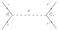
Bs0superscriptsubscript𝐵𝑠0B_{s}^{0} meson decays into charged muons μ+μsuperscript𝜇superscript𝜇\mu^{+}\mu^{-} are very interesting due to their sensitivity to BSM theories. One of which is the THDM; in this scenario the process Bs0μ+μsuperscriptsubscript𝐵𝑠0superscript𝜇superscript𝜇B_{s}^{0}\to\mu^{+}\mu^{-}, is mediated by a neutral Higgs boson, whose Feynman graph at the quark level is shown in Fig. 2.
Refer to caption
Figure 2: Feynman diagram for the Bs0μ+μsuperscriptsubscript𝐵𝑠0superscript𝜇superscript𝜇B_{s}^{0}\to\mu^{+}\mu^{-} process at the tree level, where H=h0,H0,A0𝐻superscript0superscript𝐻0superscript𝐴0H=h^{0},\,H^{0},\,A^{0}. The labels ηff¯Hsuperscriptsubscript𝜂𝑓¯𝑓𝐻\eta_{f\bar{f}}^{H} indicate the contributions coming from the THDM-Tx. We omit these labels in all further Feynman diagrams.

This decay is particularly important because impose stringent constraints on several theories beyond the SM. The first observation of the rare Bs0μμ+superscriptsubscript𝐵𝑠0superscript𝜇superscript𝜇B_{s}^{0}\to\mu^{-}\mu^{+} decay at the LHC by the CMS and LHCb experiments [36] reported a result of its branching ratio, whose value is

BR(Bs0μ+μ)=(2.80.6+0.7)×109,𝐵𝑅superscriptsubscript𝐵𝑠0superscript𝜇superscript𝜇superscriptsubscript2.80.60.7superscript109BR(B_{s}^{0}\rightarrow\mu^{+}\mu^{-})=(2{.}8_{-0{.}6}^{+0{.}7})\times 10^{-9}, (72)

while the SM value reported by [37] is

BR(Bs0μ+μ)SM=(3.23±0.27)×109.𝐵𝑅subscriptsuperscriptsubscript𝐵𝑠0superscript𝜇superscript𝜇𝑆𝑀plus-or-minus3.230.27superscript109BR(B_{s}^{0}\rightarrow\mu^{+}\mu^{-})_{SM}=(3{.}23\pm 0{.}27)\times 10^{-9}. (73)

The branching ratio for this decay is given by [38],

BR(Bsμ+μ)𝐵𝑅subscript𝐵𝑠superscript𝜇superscript𝜇\displaystyle BR\left(B_{s}\rightarrow\mu^{+}\mu^{-}\right) =\displaystyle= GF2αem216π3MBτB|VtsVtb|214mμ2MB2superscriptsubscript𝐺𝐹2superscriptsubscript𝛼𝑒𝑚216superscript𝜋3subscript𝑀𝐵subscript𝜏𝐵superscriptsubscript𝑉𝑡𝑠superscriptsubscript𝑉𝑡𝑏214superscriptsubscript𝑚𝜇2superscriptsubscript𝑀𝐵2\displaystyle\frac{G_{F}^{2}\alpha_{em}^{2}}{16\pi^{3}}M_{B}\tau_{B}\left|V_{ts}V_{tb}^{*}\right|^{2}\sqrt{1-\frac{4m_{\mu}^{2}}{M_{B}^{2}}} (74)
×\displaystyle\times [|FRH|2(14mμ2MB2)+|FRA0|2],delimited-[]superscriptsubscript𝐹𝑅𝐻214superscriptsubscript𝑚𝜇2superscriptsubscript𝑀𝐵2superscriptsubscript𝐹𝑅superscript𝐴02\displaystyle\left[\left|F_{RH}\right|^{2}\left(1-\frac{4m_{\mu}^{2}}{M_{B}^{2}}\right)+\left|F_{RA^{0}}\right|^{2}\right],

where

FRH,RA0=i2MB2fBbmb(mb+ms)mμCRH,RA0,subscript𝐹𝑅𝐻𝑅superscript𝐴0𝑖2superscriptsubscript𝑀𝐵2subscript𝑓subscript𝐵𝑏subscript𝑚𝑏subscript𝑚𝑏subscript𝑚𝑠subscript𝑚𝜇subscript𝐶𝑅𝐻𝑅superscript𝐴0F_{RH,RA^{0}}=-\frac{i}{2}M_{B}^{2}\,f_{B_{b}}\frac{m_{b}}{(m_{b}+m_{s})m_{\mu}}C_{RH,RA^{0}}, (75)

are the form factors, GFsubscript𝐺𝐹G_{F} is the Fermi constant, τBsubscript𝜏𝐵\tau_{B} is the lifetime of the B𝐵B meson, fBbsubscript𝑓subscript𝐵𝑏f_{B_{b}} is the meson decay constant and CRHsubscript𝐶𝑅𝐻C_{RH}, CRA0subscript𝐶𝑅superscript𝐴0C_{RA^{0}} are the Wilson coefficients that appear in the effective Hamiltonian,

Heff=22GFVtbVtbiCiQi,subscript𝐻𝑒𝑓𝑓22subscript𝐺𝐹subscript𝑉𝑡𝑏superscriptsubscript𝑉𝑡𝑏subscript𝑖subscript𝐶𝑖subscript𝑄𝑖H_{eff}=-2\sqrt{2}G_{F}V_{tb}V_{tb}^{*}\sum_{i}C_{i}Q_{i}, (76)

where Qisubscript𝑄𝑖Q_{i} are the effective operators with i=RH,RA0𝑖𝑅𝐻𝑅superscript𝐴0i=RH,RA^{0}:

QRHsubscript𝑄𝑅𝐻\displaystyle Q_{RH} =\displaystyle= e216π2(s¯PRb)(μ+μ),superscript𝑒216superscript𝜋2¯𝑠subscript𝑃𝑅𝑏superscript𝜇superscript𝜇\displaystyle\frac{e^{2}}{16\pi^{2}}(\bar{s\,}P_{R}b)({\mu^{+}}\,\mu^{-}), (77)
QRA0subscript𝑄𝑅superscript𝐴0\displaystyle Q_{RA^{0}} =\displaystyle= e216π2(s¯PRb)(μ+γ5μ),superscript𝑒216superscript𝜋2¯𝑠subscript𝑃𝑅𝑏superscript𝜇superscript𝛾5superscript𝜇\displaystyle\frac{e^{2}}{16\pi^{2}}(\bar{s\,}P_{R}b)({\mu^{+}}\gamma^{5}\mu^{-}), (78)

and the Wilson coefficients Cisubscript𝐶𝑖C_{i} are,

CRHsubscript𝐶𝑅𝐻\displaystyle C_{RH} =\displaystyle= 2πmμ2VtsVtbαem[14mH02H=H0,h0ηb¯sHημμ+H],2𝜋superscriptsubscript𝑚𝜇2superscriptsubscript𝑉𝑡𝑠subscript𝑉𝑡𝑏subscript𝛼𝑒𝑚delimited-[]14superscriptsubscript𝑚superscript𝐻02subscript𝐻superscript𝐻0superscript0superscriptsubscript𝜂¯𝑏𝑠𝐻superscriptsubscript𝜂superscript𝜇superscript𝜇𝐻\displaystyle\frac{2\pi m_{\mu}^{2}}{V_{ts}^{*}V_{tb}\alpha_{em}}\Bigg{[}\frac{1}{4m_{H^{0}}^{2}}\sum_{H=H^{0},\,h^{0}}\eta_{\bar{b}s}^{H}\eta_{\mu^{-}\mu^{+}}^{H}\Bigg{]}, (79)
CRA0=2πmμ2VtsVtbαem[14mA02ηb¯sA0ημμ+A0].subscript𝐶𝑅superscript𝐴02𝜋superscriptsubscript𝑚𝜇2superscriptsubscript𝑉𝑡𝑠subscript𝑉𝑡𝑏subscript𝛼𝑒𝑚delimited-[]14superscriptsubscript𝑚superscript𝐴02superscriptsubscript𝜂¯𝑏𝑠superscript𝐴0superscriptsubscript𝜂superscript𝜇superscript𝜇superscript𝐴0\displaystyle C_{RA^{0}}=\frac{2\pi m_{\mu}^{2}}{V_{ts}^{*}V_{tb}\alpha_{em}}\Bigg{[}\frac{1}{4m_{A^{0}}^{2}}\eta_{\bar{b}s}^{A^{0}}\eta_{\mu^{-}\mu^{+}}^{A^{0}}\Bigg{]}. (80)

Here mb,Vtb(ts),MH0,Mh0,MA0subscript𝑚𝑏subscriptsuperscript𝑉𝑡𝑏𝑡𝑠subscript𝑀superscript𝐻0subscript𝑀superscript0subscript𝑀superscript𝐴0m_{b},\,V^{*}_{tb(ts)},M_{H^{0}},M_{h^{0}},M_{A^{0}} are the bottom quark mass, CKM elements and Higgs boson masses, respectively. Operators with Left-handed b-quarks are parametrically suppressed compared to those involving Right-handed by a factor mssubscript𝑚𝑠m_{s}/mbsubscript𝑚𝑏m_{b}. Therefore, they are sub-leading corrections for our work. However there are some cases where these corrections are important, for instance when you have a complete general flavor violating MSSM. See for example section II of Ref.[38] for the complete effective Hamiltonian and the Wilson coefficients.We observe from 79-80 the dependence on the model parameters.

IV.2 aμTHDMTxsuperscriptsubscript𝑎𝜇𝑇𝐻𝐷𝑀𝑇𝑥a_{\mu}^{THDM-Tx}

There currently exists a discrepancy between the experimental measurement and the theoretical prediction of aμsubscript𝑎𝜇a_{\mu} in the SM [34]

Δaμ=aμExpaμSM=288(63)(49)×1011,Δsubscript𝑎𝜇superscriptsubscript𝑎𝜇𝐸𝑥𝑝superscriptsubscript𝑎𝜇𝑆𝑀2886349superscript1011\displaystyle\Delta a_{\mu}=a_{\mu}^{Exp}-a_{\mu}^{SM}=288(63)(49)\times 10^{-11}, (81)

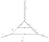
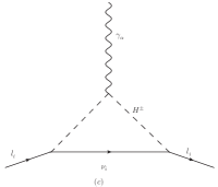
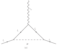
which is greater than 3σ𝜎\sigma, this discrepancy might originate from physics beyond the SM. That is why it is important to implement it to constrain new models, such as in the case of the THDM-Tx; in this model new contributions to aμsubscript𝑎𝜇a_{\mu} come from one the loop level couplings h0μlsuperscript0𝜇𝑙h^{0}\mu l, H0μlsuperscript𝐻0𝜇𝑙H^{0}\mu l, A0μlsuperscript𝐴0𝜇𝑙A^{0}\mu l, where l=e,μ,τ𝑙𝑒𝜇𝜏l=e,\,\mu,\,\tau.

The Feynman diagrams for these one loop level processes are shown in FIG. 3
Refer to caption
(a)
Refer to caption
(b)
Refer to caption
(c)
Figure 3: Feynman diagrams of the muon anomalous magnetic dipole moment.

Where li=μsubscript𝑙𝑖𝜇l_{i}=\mu and ljsubscript𝑙𝑗l_{j} is a different flavored lepton, H𝐻H refers to the different neutral Higgs bosons h0,H0,A0superscript0superscript𝐻0superscript𝐴0h^{0},H^{0},A^{0}. The muon anomalous magnetic dipole moment is CP-conserving, thus α1, 2=0subscript𝛼120\alpha_{1,\,2}=0.

We use the unitary gauge and the method of Feynman parametrization. The expressions for the aμTHDMTxsuperscriptsubscript𝑎𝜇𝑇𝐻𝐷𝑀𝑇𝑥a_{\mu}^{THDM-Tx}, at one-loop level, are given by:

aμTHDMTx=l=e,μ,τl=μ|ηllH|2mμ8π201𝑑x01x𝑑yFk(x,y),superscriptsubscript𝑎𝜇𝑇𝐻𝐷𝑀𝑇𝑥superscript𝑙𝜇𝑙𝑒𝜇𝜏superscriptsuperscriptsubscript𝜂𝑙superscript𝑙𝐻2subscript𝑚𝜇8superscript𝜋2superscriptsubscript01differential-d𝑥superscriptsubscript01𝑥differential-d𝑦subscript𝐹𝑘𝑥𝑦a_{\mu}^{THDM-Tx}=\underset{\underset{l^{\prime}=\mu}{l=e,\,\mu,\,\tau}}{\sum}\frac{\left|\eta_{{}_{ll^{\prime}}}^{H}\right|^{2}m_{\mu}}{\sqrt{8}\pi^{2}}\intop_{0}^{1}dx\intop_{0}^{1-x}dy\,F_{k}(x,\,y), (82)

where ηllHsuperscriptsubscript𝜂𝑙superscript𝑙𝐻\eta_{{}_{ll^{\prime}}}^{H} is the coupling ll¯H𝑙¯𝑙𝐻l\bar{l}H that comes from the neutral Lagrangian, Eq. 69.

The Fk(x,y)subscript𝐹𝑘𝑥𝑦F_{k}(x,\,y) function of diagram (a) is given by:

Fa(x,y)=(x+y)(mljmμ(x+y1))/Ma2,subscript𝐹𝑎𝑥𝑦𝑥𝑦subscript𝑚subscript𝑙𝑗subscript𝑚𝜇𝑥𝑦1superscriptsubscript𝑀𝑎2F_{a}(x,\,y)=(x+y)(m_{l_{j}}-m_{\mu}(x+y-1))/M_{a}^{2}, (83)

where Ma2=mH2(x+y1)+(x+y)(mlj2+mμ2(x+y1)M_{a}^{2}=-m_{H}^{2}(x+y-1)+(x+y)(m_{l_{j}}^{2}+m_{\mu}^{2}(x+y-1).

For diagram (c): ηllH=1superscriptsubscript𝜂𝑙superscript𝑙𝐻1\eta_{{}_{ll^{\prime}}}^{H}=1 and

Fc(x)=2mμx/Mc2,subscript𝐹𝑐𝑥2subscript𝑚𝜇𝑥superscriptsubscript𝑀𝑐2F_{c}(x)=2m_{\mu}x/M_{c}^{2}, (84)

such that Mc2=(mμ2xmH±2)superscriptsubscript𝑀𝑐2superscriptsubscript𝑚𝜇2𝑥superscriptsubscript𝑚superscript𝐻plus-or-minus2M_{c}^{2}=(m_{\mu}^{2}x-m_{H^{\pm}}^{2}).
In the case of the Barr-Zee diagram, we only considerer the dominant contribution which is given by [35]:

aμBarrZee=α28π2sW2mμ2ημμ+A0mW2f=t,τ,bNcfQf2rff(rf)ηff¯A0,superscriptsubscript𝑎𝜇𝐵𝑎𝑟𝑟𝑍𝑒𝑒superscript𝛼28superscript𝜋2superscriptsubscript𝑠𝑊2superscriptsubscript𝑚𝜇2superscriptsubscript𝜂superscript𝜇superscript𝜇superscript𝐴0superscriptsubscript𝑚𝑊2subscript𝑓𝑡𝜏𝑏superscriptsubscript𝑁𝑐𝑓superscriptsubscript𝑄𝑓2subscript𝑟𝑓𝑓subscript𝑟𝑓superscriptsubscript𝜂𝑓¯𝑓superscript𝐴0a_{\mu}^{Barr\,Zee}=\frac{\alpha^{2}}{8\pi^{2}s_{W}^{2}}\frac{m_{\mu}^{2}\eta_{\mu^{-}\mu^{+}}^{A^{0}}}{m_{W}^{2}}\sum_{f=t,\,\tau,\,b}N_{c}^{f}Q_{f}^{2}r_{f}f(r_{f})\eta_{f\bar{f}}^{A^{0}}, (85)

where rf=(mf/MA0)subscript𝑟𝑓subscript𝑚𝑓subscript𝑀superscript𝐴0r_{f}=(m_{f}/M_{A^{0}}), mfsubscript𝑚𝑓m_{f} is the fermion mass, Ncf=1(3)superscriptsubscript𝑁𝑐𝑓13N_{c}^{f}=1(3) is the color number: in the case of leptons (quarks), Qfsubscript𝑄𝑓Q_{f} is the electric charge of fermions, ηff¯A0superscriptsubscript𝜂𝑓¯𝑓superscript𝐴0\eta_{f\bar{f}}^{A^{0}} is given by the Lagrangian in eq.68 and the function f(rf)𝑓subscript𝑟𝑓f(r_{f}) is given by

f(x)=01log(xy(1y))xy(1x)𝑑y.𝑓𝑥superscriptsubscript01𝑙𝑜𝑔𝑥𝑦1𝑦𝑥𝑦1𝑥differential-d𝑦f(x)=\int_{0}^{1}\frac{log(\frac{x}{y(1-y)})}{x-y(1-x)}dy. (86)

IV.3 Meson Mixing: KK¯𝐾¯𝐾K\bar{K} and BB¯𝐵¯𝐵B\bar{B} Mixing

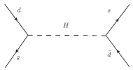
One of the earliest successful tests of SM phenomenology was the measurement of the difference between the mass eigenvalues ΔMK=MLMSΔsubscript𝑀𝐾subscript𝑀𝐿subscript𝑀𝑆\Delta M_{K}=M_{L}-M_{S}; related to M1,2Ksuperscriptsubscript𝑀12𝐾M_{1,2}^{K} which occur through box diagrams involving the W boson. But in the THDM the amplitude of KK¯𝐾¯𝐾K\bar{K} mixing receives additional contributions from the neutral scalars, whose Feynman diagram is shown in Fig. 4.
Refer to caption
Figure 4: Feynman diagram for the KK¯𝐾¯𝐾K-\bar{K} mixing.

The effective hamiltonian for this process at the quark level is written as follows

HeffΔS=2=GF2MW216π2iCiQi,superscriptsubscript𝐻𝑒𝑓𝑓Δ𝑆2superscriptsubscript𝐺𝐹2superscriptsubscript𝑀𝑊216superscript𝜋2subscript𝑖subscript𝐶𝑖subscript𝑄𝑖\displaystyle H_{eff}^{\Delta S=2}=\frac{G_{F}^{2}M_{W}^{2}}{16\pi^{2}}\sum_{i}C_{i}Q_{i}, (87)

with (i=L,R,LR)𝑖𝐿𝑅𝐿𝑅(i=L,R,LR)

QLs¯d,sd¯superscriptsubscript𝑄𝐿¯𝑠𝑑𝑠¯𝑑\displaystyle Q_{L}^{\overline{s}d,s\overline{d}} =\displaystyle= (s¯PLd)(s¯PLd),¯𝑠subscript𝑃𝐿𝑑¯𝑠subscript𝑃𝐿𝑑\displaystyle\big{(}\bar{s}P_{L}d\big{)}\big{(}\bar{s}P_{L}d\big{)}, (88)
QRs¯d,sd¯superscriptsubscript𝑄𝑅¯𝑠𝑑𝑠¯𝑑\displaystyle Q_{R}^{\overline{s}d,s\overline{d}} =\displaystyle= (s¯PRd)(s¯PRd),¯𝑠subscript𝑃𝑅𝑑¯𝑠subscript𝑃𝑅𝑑\displaystyle\big{(}\bar{s}P_{R}d\big{)}\big{(}\bar{s}P_{R}d\big{)}, (89)
QLRs¯d,sd¯superscriptsubscript𝑄𝐿𝑅¯𝑠𝑑𝑠¯𝑑\displaystyle Q_{LR}^{\overline{s}d,s\overline{d}} =\displaystyle= (s¯PLd)(s¯PRd),¯𝑠subscript𝑃𝐿𝑑¯𝑠subscript𝑃𝑅𝑑\displaystyle\big{(}\bar{s}P_{L}d\big{)}\big{(}\bar{s}P_{R}d\big{)}, (90)

and the Wilson coefficients are written here for a general multi-Higgs doublet model,

CLs¯d,sd¯=16π2GFmW2msmd|ηsdH|2a=1,H2(U1a)2mH2g,superscriptsubscript𝐶𝐿¯𝑠𝑑𝑠¯𝑑16superscript𝜋2subscript𝐺𝐹superscriptsubscript𝑚𝑊2subscript𝑚𝑠subscript𝑚𝑑superscriptsuperscriptsubscript𝜂𝑠𝑑𝐻2superscriptsubscript𝑎1𝐻2superscriptsuperscriptsubscript𝑈1𝑎2superscriptsubscript𝑚𝐻2𝑔\displaystyle C_{L}^{\overline{s}d,s\overline{d}}=-\frac{16\pi^{2}}{G_{F}m_{W}^{2}}m_{s}m_{d}|\eta_{sd}^{H}|^{2}\sum_{a=1,\,H}^{2}\frac{\big{(}U_{1a}^{*}\big{)}^{2}}{m_{H}^{2}}g, (91)
CRs¯d,sd¯=16π2GFmW2msmd|ηsdH|2a=1,H2(U1a)2mH2,superscriptsubscript𝐶𝑅¯𝑠𝑑𝑠¯𝑑16superscript𝜋2subscript𝐺𝐹superscriptsubscript𝑚𝑊2subscript𝑚𝑠subscript𝑚𝑑superscriptsuperscriptsubscript𝜂𝑠𝑑𝐻2superscriptsubscript𝑎1𝐻2superscriptsubscript𝑈1𝑎2superscriptsubscript𝑚𝐻2\displaystyle C_{R}^{\overline{s}d,s\overline{d}}=-\frac{16\pi^{2}}{G_{F}m_{W}^{2}}m_{s}m_{d}|\eta_{sd}^{H}|^{2}\sum_{a=1,\,H}^{2}\frac{\big{(}U_{1a}\big{)}^{2}}{m_{H}^{2}}, (92)
CLRs¯d,sd¯=16π2GFmW2msmd|ηsdH|2a=1,H2U1aU1amH2,superscriptsubscript𝐶𝐿𝑅¯𝑠𝑑𝑠¯𝑑16superscript𝜋2subscript𝐺𝐹superscriptsubscript𝑚𝑊2subscript𝑚𝑠subscript𝑚𝑑superscriptsuperscriptsubscript𝜂𝑠𝑑𝐻2superscriptsubscript𝑎1𝐻2superscriptsubscript𝑈1𝑎subscript𝑈1𝑎superscriptsubscript𝑚𝐻2\displaystyle C_{LR}^{\overline{s}d,s\overline{d}}=-\frac{16\pi^{2}}{G_{F}m_{W}^{2}}m_{s}m_{d}|\eta_{sd}^{H}|^{2}\sum_{a=1,\,H}^{2}\frac{U_{1a}^{*}U_{1a}}{m_{H}^{2}}, (93)

the rotation matrix for neutral Higgs bosons takes the form

U=(cosαsinαsinαcosα).𝑈matrix𝛼𝛼𝛼𝛼\displaystyle U=\begin{pmatrix}\cos\alpha&-\sin\alpha\\ \sin\alpha&\cos\alpha\\ \end{pmatrix}. (94)

Flavor violation arises from the non-diagonal terms of the K (neutral kaon) mass matrix, in particular the component M12K,superscriptsubscript𝑀12𝐾M_{12}^{K}, whose experimental value has been measured to be

M12K=ΔMKMK=7.2948×10¹⁵,superscriptsubscript𝑀12𝐾Δsubscript𝑀𝐾subscript𝑀𝐾7.2948superscript1015\displaystyle M_{12}^{K}=\frac{\Delta M_{K}}{M_{K}}=7.2948\times 10^{-15}, (95)

which is a high precision measurement that is used to constrain BSM parameters. Given that ΔMKΔsubscript𝑀𝐾\Delta M_{K} is obtained through:

ΔMKΔsubscript𝑀𝐾\displaystyle\Delta M_{K} =\displaystyle= 2ReK¯0|HeffΔS=2|K02𝑅𝑒quantum-operator-productsuperscript¯𝐾0superscriptsubscript𝐻𝑒𝑓𝑓Δ𝑆2superscript𝐾0\displaystyle 2Re\langle\bar{K}^{0}|H_{eff}^{\Delta S=2}|K^{0}\rangle
=\displaystyle= GF2MW212π2MKFK2η2BK×[P¯2,LRCLRs¯d,sd¯+P¯1,L(CLs¯d,sd¯+CRs¯d,sd¯)],superscriptsubscript𝐺𝐹2superscriptsubscript𝑀𝑊212superscript𝜋2subscript𝑀𝐾superscriptsubscript𝐹𝐾2subscript𝜂2subscript𝐵𝐾delimited-[]subscript¯𝑃2𝐿𝑅superscriptsubscript𝐶𝐿𝑅¯𝑠𝑑𝑠¯𝑑subscript¯𝑃1𝐿superscriptsubscript𝐶𝐿¯𝑠𝑑𝑠¯𝑑superscriptsubscript𝐶𝑅¯𝑠𝑑𝑠¯𝑑\displaystyle\frac{G_{F}^{2}M_{W}^{2}}{12\pi^{2}}M_{K}F_{K}^{2}\eta_{2}{B}_{K}\times\left[\bar{P}_{2,LR}C_{LR}^{\overline{s}d,s\overline{d}}+\bar{P}_{1,L}\left(C_{L}^{\overline{s}d,s\overline{d}}+C_{R}^{\overline{s}d,s\overline{d}}\right)\right],

where FK=160subscript𝐹𝐾160F_{K}=160 MeV, MK=497.6subscript𝑀𝐾497.6M_{K}=497.6 MeV, η2=0.57,BK=0.85±0.15,P¯2,LR=30.6formulae-sequencesubscript𝜂20.57formulae-sequencesubscript𝐵𝐾plus-or-minus0.850.15subscript¯𝑃2𝐿𝑅30.6\eta_{2}=0.57,\;\;{B}_{K}=0.85\pm 0.15,\;\;\bar{P}_{2,LR}=30.6 and P¯1,L=9.3,subscript¯𝑃1𝐿9.3\bar{P}_{1,L}=-9.3, therefore,

M𝑀\displaystyle M =12K43FK2η2B¯K(mdms)1v12×a=13[P¯2,LRU2aU1amH2+P¯1,L(U2a2mH2+U1a2mH2)].{}_{12}^{K}=\frac{4}{3}F^{2}_{K}\eta_{2}\bar{B}_{K}\big{(}m_{d}m_{s}\big{)}\frac{1}{v_{1}^{2}}\times\sum_{a=1}^{3}\bigg{[}\bar{P}_{2,LR}\frac{U_{2a}U_{1a}}{m_{H}^{2}}+\bar{P}_{1,L}\bigg{(}\frac{U_{2a}^{2}}{m_{H}^{2}}+\frac{U_{1a}^{2}}{m_{H}^{2}}\bigg{)}\bigg{]}. (97)

The way in which we determine BB¯𝐵¯𝐵B-\bar{B} mixing is analogous to KK¯𝐾¯𝐾K\bar{K} mixing, except that we now use ΔMBΔsubscript𝑀𝐵\Delta M_{B}. For this process the experimental values used are ΔmBs=3.337×10¹³Δsubscript𝑚subscript𝐵𝑠3.337superscript1013\Delta m_{B_{s}}=3.337\times 10^{-13} GeV, ηB=0.55,P¯2,LR=0.88formulae-sequencesubscript𝜂𝐵0.55subscript¯𝑃2𝐿𝑅0.88\eta_{B}=0.55,\;\;\bar{P}_{2,LR}=0.88 and P¯1,L=0.52subscript¯𝑃1𝐿0.52\bar{P}_{1,L}=-0.52.

IV.4 BDτν𝐵𝐷𝜏𝜈B\rightarrow D\tau\nu and BDτν𝐵superscript𝐷𝜏𝜈B\rightarrow D^{\star}\tau\nu

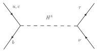
The experiments Belle and BaBar have now measured the ratios R(D𝐷D) and R(Dsuperscript𝐷D^{\star}) [39, 40], of BDτν𝐵𝐷𝜏𝜈B\rightarrow D\tau\nu and BDτν𝐵superscript𝐷𝜏𝜈B\rightarrow D^{\star}\tau\nu; which can be used to constrain charged Higgs H±superscript𝐻plus-or-minusH^{\pm} parameters appearing in models such as in the case of the THDM-Tx. The Feynman diagram corresponding to this process is shown in Fig. 5,
Refer to caption
Figure 5: Feynman diagram for the BD(D)τν𝐵𝐷superscript𝐷𝜏𝜈B\rightarrow D(D^{*})\tau\nu process.

the results given by BaBar are:

R(D)𝑅𝐷\displaystyle R(D) =\displaystyle= 0.44±0.058±0.042,plus-or-minus0.440.0580.042\displaystyle 0.44\pm 0.058\pm 0.042, (98)
R(D)𝑅superscript𝐷\displaystyle R(D^{*}) =\displaystyle= 0.332±0.024±0.018,plus-or-minus0.3320.0240.018\displaystyle 0.332\pm 0.024\pm 0.018,

which can be expressed as follows,

R(D)=RSM(D)(1+1.5Re[CRcb,τν+CLcb,τνCSMcb,τν]+1.0|CRcb,τν+CLcb,τνCSMcb,τν|2),𝑅𝐷subscript𝑅𝑆𝑀𝐷11.5Redelimited-[]superscriptsubscript𝐶𝑅𝑐𝑏𝜏𝜈superscriptsubscript𝐶𝐿𝑐𝑏𝜏𝜈superscriptsubscript𝐶𝑆𝑀𝑐𝑏𝜏𝜈1.0superscriptsuperscriptsubscript𝐶𝑅𝑐𝑏𝜏𝜈superscriptsubscript𝐶𝐿𝑐𝑏𝜏𝜈superscriptsubscript𝐶𝑆𝑀𝑐𝑏𝜏𝜈2{R}(D)={R}_{SM}(D)\Big{(}1+1.5\;{\mbox{Re}}\left[\frac{C_{R}^{cb\,,\tau\nu}+C_{L}^{cb\,,\tau\nu}}{C_{SM}^{cb\,,\tau\nu}}\right]\\ +1.0\left|\frac{C_{R}^{cb\,,\tau\nu}+C_{L}^{cb\,,\tau\nu}}{C_{SM}^{cb\,,\tau\nu}}\right|^{2}\Big{)}\,,
R(D)=RSM(D)(1+0.12Re[CRcb,τνCLcb,τνCSMcb,τν]+0.05|CRcb,τνCLcb,τνCSMcb,τν|2),𝑅superscript𝐷subscript𝑅𝑆𝑀superscript𝐷10.12Redelimited-[]superscriptsubscript𝐶𝑅𝑐𝑏𝜏𝜈superscriptsubscript𝐶𝐿𝑐𝑏𝜏𝜈superscriptsubscript𝐶𝑆𝑀𝑐𝑏𝜏𝜈0.05superscriptsuperscriptsubscript𝐶𝑅𝑐𝑏𝜏𝜈superscriptsubscript𝐶𝐿𝑐𝑏𝜏𝜈superscriptsubscript𝐶𝑆𝑀𝑐𝑏𝜏𝜈2{R}(D^{*})={R}_{SM}(D^{*})\Big{(}1+0.12\;{\mbox{Re}}\left[\frac{C_{R}^{cb\,,\tau\nu}-C_{L}^{cb\,,\tau\nu}}{C_{SM}^{cb\,,\tau\nu}}\right]\ +0.05\left|\frac{C_{R}^{cb\,,\tau\nu}-C_{L}^{cb\,,\tau\nu}}{C_{SM}^{cb\,,\tau\nu}}\right|^{2}\Big{)}\,, (99)

where the Wilson coefficients are given in Ref. [41].

The combination of both processes give us a deviation of 3.4 σ𝜎\sigma with respect to SM predictions; it remains to be seen if this is in fact a signal of new physics.

This signal is one of the most stringent processes. Nonetheless, we are able to satisfy both R(D)𝑅𝐷R(D) and R(D)𝑅superscript𝐷R(D^{\star}) within of THDM-Tx. The allowed and excluded regions for tanβ𝛽\tan\beta-MH±subscript𝑀superscript𝐻plus-or-minusM_{H^{\pm}} plane are presented in IV.7

IV.5 Lepton decays liljγsubscript𝑙𝑖subscript𝑙𝑗𝛾l_{i}\to l_{j}\gamma

Another way in which one may constrain the parameter space of a model is through the consideration of radiative flavor violating decays, such as in the case of leptonic decays of which μeγ𝜇𝑒𝛾\mu\to e\gamma is particularly useful. The MEG collaboration [42] has given an upper bound for the decay μeγ𝜇𝑒𝛾\mu\to e\gamma: 5.7×10135.7superscript10135.7\times 10^{-13}, they also give bounds of the leptonic decays of the τ𝜏\tau but they are much weaker: BR(τeγ)𝜏𝑒𝛾(\tau\to e\gamma)=3.3×1083.3superscript1083.3\times 10^{-8} and BR(τμγ)𝜏𝜇𝛾(\tau\to\mu\gamma)=4.43×1084.43superscript1084.43\times 10^{-8} [43]. That is why in the present work we only used μeγ𝜇𝑒𝛾\mu\to e\gamma to constrain our parameter space.

The Feynman diagram for this process is shown in Fig. 6,

Refer to caption
Figure 6: Feynman diagram for the liljγsubscript𝑙𝑖subscript𝑙𝑗𝛾l_{i}\to l_{j}\gamma process with H=H0,h0,A0,H±𝐻superscript𝐻0superscript0superscript𝐴0superscript𝐻plus-or-minusH=H^{0},h^{0},A^{0},H^{\pm}. The circle denotes one-loop contributions.

The branching ratio for the general decay of a lepton (lisubscript𝑙𝑖l_{i}) to a lepton of a different family (ljsubscript𝑙𝑗l_{j}) is given by

BR(liljγ)=mli54πΓli(|CRljli|2+|CLljli|2),𝐵𝑅subscript𝑙𝑖subscript𝑙𝑗𝛾superscriptsubscript𝑚subscript𝑙𝑖54𝜋subscriptΓsubscript𝑙𝑖superscriptsuperscriptsubscript𝐶𝑅subscript𝑙𝑗subscript𝑙𝑖2superscriptsuperscriptsubscript𝐶𝐿subscript𝑙𝑗subscript𝑙𝑖2\displaystyle BR(l_{i}\to l_{j}\gamma)=\frac{m_{l_{i}}^{5}}{4\pi\Gamma_{l_{i}}}\left(\big{|}C_{R}^{l_{j}l_{i}}\big{|}^{2}+\big{|}C_{L}^{l_{j}l_{i}}\big{|}^{2}\right), (100)

where ΓlisubscriptΓsubscript𝑙𝑖\Gamma_{l_{i}} is the total decay width of the particle lisubscript𝑙𝑖l_{i} and the Wilson Coefficients CR,Lljlisuperscriptsubscript𝐶𝑅𝐿subscript𝑙𝑗subscript𝑙𝑖C_{R,L}^{l_{j}l_{i}} are given by

CRljlisuperscriptsubscript𝐶𝑅subscript𝑙𝑗subscript𝑙𝑖\displaystyle C_{R}^{l_{j}l_{i}} =\displaystyle= He192π2MH2subscript𝐻𝑒192superscript𝜋2superscriptsubscript𝑀𝐻2\displaystyle\sum_{H}\frac{-e}{192\pi^{2}M_{H}^{2}} (101)
[ηliljLRHηliljLRH+ηljliLRHηljliLRHmlimljηliljLRHηljliLRH(9+6ln(mlj2mH2))],delimited-[]superscriptsubscript𝜂subscript𝑙𝑖subscript𝑙𝑗𝐿𝑅𝐻superscriptsubscript𝜂subscript𝑙𝑖subscript𝑙𝑗𝐿𝑅𝐻superscriptsubscript𝜂subscript𝑙𝑗subscript𝑙𝑖𝐿𝑅𝐻superscriptsubscript𝜂subscript𝑙𝑗subscript𝑙𝑖𝐿𝑅𝐻subscript𝑚subscript𝑙𝑖subscript𝑚subscript𝑙𝑗superscriptsubscript𝜂subscript𝑙𝑖subscript𝑙𝑗𝐿𝑅𝐻superscriptsubscript𝜂subscript𝑙𝑗subscript𝑙𝑖𝐿𝑅𝐻96superscriptsubscript𝑚subscript𝑙𝑗2superscriptsubscript𝑚𝐻2\displaystyle\Bigg{[}\eta_{l_{i}l_{j}}^{LRH\star}\eta_{l_{i}l_{j}}^{LRH}+\eta_{l_{j}l_{i}}^{LRH\star}\eta_{l_{j}l_{i}}^{LRH}-\frac{m_{l_{i}}}{m_{l_{j}}}\eta_{l_{i}l_{j}}^{LRH}\eta_{l_{j}l_{i}}^{LRH}\left(9+6\ln\left(\frac{m_{l_{j}}^{2}}{m_{H}^{2}}\right)\right)\Bigg{]},

such that H=h0,H0,A0𝐻superscript0superscript𝐻0superscript𝐴0H=h^{0},H^{0},A^{0}. CLljlisuperscriptsubscript𝐶𝐿subscript𝑙𝑗subscript𝑙𝑖C_{L}^{l_{j}l_{i}} is obtained by simply interchanging R by L. For the charged Higgs boson contributions the Wilson Coefficients are given by:

CLljlisuperscriptsubscript𝐶𝐿subscript𝑙𝑗subscript𝑙𝑖\displaystyle C_{L}^{l_{j}l_{i}} =\displaystyle= e384π2MH±2k=13ξνkliLξνkljL,𝑒384superscript𝜋2superscriptsubscript𝑀superscript𝐻plus-or-minus2superscriptsubscript𝑘13superscriptsubscript𝜉subscript𝜈𝑘subscript𝑙𝑖𝐿superscriptsubscript𝜉subscript𝜈𝑘subscript𝑙𝑗𝐿\displaystyle\frac{e}{384\pi^{2}M_{H^{\pm}}^{2}}{\sum_{k=1}^{3}}\xi_{\nu_{k}l_{i}}^{L}\xi_{\nu_{k}l_{j}}^{L}, (102)
CRljlisuperscriptsubscript𝐶𝑅subscript𝑙𝑗subscript𝑙𝑖\displaystyle C_{R}^{l_{j}l_{i}} =\displaystyle= mljmlie384π2MH±2k=13ξνkliRξνkljR,subscript𝑚subscript𝑙𝑗subscript𝑚subscript𝑙𝑖𝑒384superscript𝜋2superscriptsubscript𝑀superscript𝐻plus-or-minus2superscriptsubscript𝑘13superscriptsubscript𝜉subscript𝜈𝑘subscript𝑙𝑖𝑅superscriptsubscript𝜉subscript𝜈𝑘subscript𝑙𝑗𝑅\displaystyle\frac{m_{l_{j}}}{m_{l_{i}}}\frac{e}{384\pi^{2}M_{H^{\pm}}^{2}}{\sum_{k=1}^{3}}\xi_{\nu_{k}l_{i}}^{R}\xi_{\nu_{k}l_{j}}^{R}, (103)

where

ξνkliL,R=m=13sinβVkmPMNS(ϵmitanβ),superscriptsubscript𝜉subscript𝜈𝑘subscript𝑙𝑖𝐿𝑅superscriptsubscript𝑚13𝛽superscriptsubscript𝑉𝑘𝑚𝑃𝑀𝑁𝑆subscriptitalic-ϵ𝑚𝑖𝛽\xi_{\nu_{k}l_{i}}^{L,R}=-{\sum_{m=1}^{3}}\sin\beta\,V_{km}^{PMNS}(\epsilon_{mi}\tan\beta),

with

|ϵmi|(2.9×1066.1×1041.0×1026.1×1046.1×1041.0×1021.0×1021.0×1021.0×102).subscriptitalic-ϵ𝑚𝑖2.9superscript1066.1superscript1041.0superscript1026.1superscript1046.1superscript1041.0superscript1021.0superscript1021.0superscript1021.0superscript102|\epsilon_{mi}|\leq\left(\begin{array}[]{ccc}2.9\times 10^{-6}&6.1\times 10^{-4}&1.0\times 10^{-2}\\ 6.1\times 10^{-4}&6.1\times 10^{-4}&1.0\times 10^{-2}\\ 1.0\times 10^{-2}&1.0\times 10^{-2}&1.0\times 10^{-2}\end{array}\right).

IV.6 τμμ+μsuperscript𝜏superscript𝜇superscript𝜇superscript𝜇\tau^{-}\rightarrow\mu^{-}\mu^{+}\mu^{-}

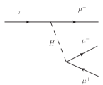
The Feynman diagram is shown in the FIG.[7],
Refer to caption
Figure 7: Feynman diagram for the τμμ+μsuperscript𝜏superscript𝜇superscript𝜇superscript𝜇\tau^{-}\rightarrow\mu^{-}\mu^{+}\mu^{-} process.

The branching ratio including contributions from the three Higgs bosons is given by:

BR(li\displaystyle BR(l_{i} \displaystyle\rightarrow ljlklk)=5δlllk+23τi211π3mljmlk2mli6v4{cos2(αβ)sin2αmh04\displaystyle l_{j}l_{k}{l}_{k})=\frac{5\delta_{l_{l}l_{k}}+2}{3}\frac{\tau_{i}}{2^{11}\pi^{3}}\frac{m_{l_{j}}m_{l_{k}}^{2}m_{l_{i}}^{6}}{v^{4}}\left\{\frac{\cos^{2}(\alpha-\beta)sin^{2}\alpha}{m_{h^{0}}^{4}}\right. (104)
+\displaystyle+ sin2(αβ)cos2αmH042cos(αβ)sin(αβ)cosαsinαmh02mH02superscript2𝛼𝛽superscript2𝛼superscriptsubscript𝑚superscript𝐻042𝛼𝛽𝛼𝛽𝛼𝛼superscriptsubscript𝑚superscript02superscriptsubscript𝑚superscript𝐻02\displaystyle\frac{\sin^{2}(\alpha-\beta)\cos^{2}\alpha}{m_{H^{0}}^{4}}-2\frac{\cos(\alpha-\beta)\sin(\alpha-\beta)\,\cos\alpha\,\sin\alpha}{m_{h^{0}}^{2}m_{H^{0}}^{2}}
+\displaystyle+ sin2βmA04}|ηij|22cos4β.\displaystyle\left.\frac{\sin^{2}\beta}{m_{A^{0}}^{4}}\right\}\frac{\left|\eta_{{ij}}\right|^{2}}{2\cos^{4}\beta}.

Here τisubscript𝜏𝑖\tau_{i} is the time life of the lisubscript𝑙𝑖l_{i} particle. The current bound is [30]:

BR(τμμ+μ)𝐵𝑅superscript𝜏superscript𝜇superscript𝜇superscript𝜇\displaystyle BR(\tau^{-}\rightarrow\mu^{-}\mu^{+}\mu^{-}) <\displaystyle< 2.1×108.2.1superscript108\displaystyle 2{.}1\times 10^{-8}.

IV.7 Allowed regions

IV.7.1 Neutral Higgs Mediated Process

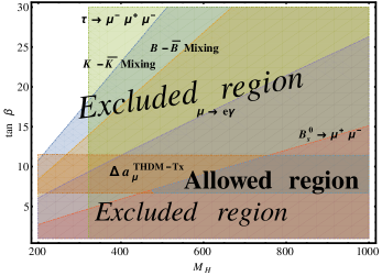
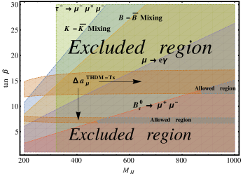
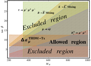
We give bounds on the tanβ𝛽\tan\beta-MHsubscript𝑀𝐻M_{H} plane. We find that not all values of MHsubscript𝑀𝐻M_{H} and tβsubscript𝑡𝛽t_{\beta} are allowed. In Fig.8 we show the allowed and excluded regions for processes that involve the neutral Higgs bosons for the complementary case, i.e. Bs0μμ+superscriptsubscript𝐵𝑠0superscript𝜇superscript𝜇B_{s}^{0}\to\mu^{-}\mu^{+}, KK¯(BB¯)𝐾¯𝐾𝐵¯𝐵K-\bar{K}(B-\bar{B}) mixing, liljγsubscript𝑙𝑖subscript𝑙𝑗𝛾l_{i}\to l_{j}\gamma, τμμ+μsuperscript𝜏superscript𝜇superscript𝜇superscript𝜇\tau^{-}\rightarrow\mu^{-}\mu^{+}\mu^{-} and aμTHDMTxsuperscriptsubscript𝑎𝜇𝑇𝐻𝐷𝑀𝑇𝑥a_{\mu}^{THDM-Tx}, where the region where they all intersect corresponds to the allowed region for all the process that we considered. We work in the scenario where (αβ)=π/2𝛼𝛽𝜋2(\alpha-\beta)=\pi/2 which is in accordance with the work of Ref. [33]. In Fig.9 we consider the same low energy processes but for the Semi-Parallel case. Finally in Fig. 10 we show the excluded and allowed region for the parallel case.
Refer to caption
Figure 8: Allowed and excluded regions of tβsubscript𝑡𝛽t_{\beta} and MHsubscript𝑀𝐻M_{H}(GeV) for the complementary case.

The labels for each process are placed at the upper limits for each process, which extends all the way down to (MH=200subscript𝑀𝐻200M_{H}=200GeV-tanβ=1𝛽1\tan{\beta}=1)-(MH=1000subscript𝑀𝐻1000M_{H}=1000GeV-tanβ=1𝛽1\tan{\beta}=1). For example, for the process Bs0μμ+superscriptsubscript𝐵𝑠0superscript𝜇superscript𝜇B_{s}^{0}\to\mu^{-}\mu^{+} the allowed region starts at (MH=200subscript𝑀𝐻200M_{H}=200GeV, tanβ=3similar-toabsent𝛽3\sim\tan{\beta}=3) and continues until (MH=1000subscript𝑀𝐻1000M_{H}=1000GeV, tanβ=15similar-toabsent𝛽15\sim\tan{\beta}=15) and extends up to (MH=200subscript𝑀𝐻200M_{H}=200GeV, tanβ=1𝛽1\tan{\beta}=1)-(MH=1000subscript𝑀𝐻1000M_{H}=1000GeV, tanβ=1𝛽1\tan{\beta}=1). The allowed regions that are different are: aμTHDMTxsuperscriptsubscript𝑎𝜇𝑇𝐻𝐷𝑀𝑇𝑥a_{\mu}^{THDM-Tx} which is a band which goes through the plot and τμμμ+superscript𝜏superscript𝜇superscript𝜇superscript𝜇\tau^{-}\to\mu^{-}\mu^{-}\mu^{+} which looks like a rectangle. Here MH=MH0subscript𝑀𝐻subscript𝑀superscript𝐻0M_{H}=M_{H^{0}} is the heavy Higgs boson mass. We used the values Mh0=125subscript𝑀superscript0125M_{h^{0}}=125 GeV, MA0=300subscript𝑀superscript𝐴0300M_{A^{0}}=300 GeV, MH±=500subscript𝑀superscript𝐻plus-or-minus500M_{H^{\pm}}=500 GeV, γu=0.13subscript𝛾𝑢0.13\gamma_{u}=0.13, γd=0.1subscript𝛾𝑑0.1\gamma_{d}=0.1 and γl=1subscript𝛾𝑙1\gamma_{l}=1. From the plot we observe that the most restrictive process in the tanβ𝛽\tan{\beta}-MHsubscript𝑀𝐻M_{H} plane are Bs0μμ+superscriptsubscript𝐵𝑠0superscript𝜇superscript𝜇B_{s}^{0}\to\mu^{-}\mu^{+} and aμTHDMTxsuperscriptsubscript𝑎𝜇𝑇𝐻𝐷𝑀𝑇𝑥a_{\mu}^{THDM-Tx}. The intersected area for all the processes corresponds to the allowed region, which is found to be between 490MH1000less-than-or-similar-to490subscript𝑀𝐻1000490\lesssim M_{H}\leq 1000 GeV for tβ7similar-tosubscript𝑡𝛽7t_{\beta}\sim 7 and 850MH1000less-than-or-similar-to850subscript𝑀𝐻1000850\lesssim M_{H}\leq 1000 for tanβ13similar-to𝛽13\tan{\beta}\sim 13.

Refer to caption
Figure 9: We now perform a similar analysis as in Fig. 8 but for the Semi-Parallel case.

Although both complementary and Semi-Parallel cases are similar, we observe that the allowed regions differ slightly, this is due to in the Semi-Parallel case there is an additional parameter (a1subscript𝑎1a_{1}). The most restrictive processes are (Bs0μμ+superscriptsubscript𝐵𝑠0superscript𝜇superscript𝜇B_{s}^{0}\to\mu^{-}\mu^{+} and aμTHDMTxsuperscriptsubscript𝑎𝜇𝑇𝐻𝐷𝑀𝑇𝑥a_{\mu}^{THDM-Tx}) just like in the previous plot. Nonetheless, the overall allowed region is greater than the complementary case, in particular for tβ13similar-tosubscript𝑡𝛽13t_{\beta}\sim 13 the Heavy Higgs boson mass is between 750MH1000less-than-or-similar-to750subscript𝑀𝐻1000750\lesssim M_{H}\leq 1000 GeV unlike the complementary case is between 850MH1000less-than-or-similar-to850subscript𝑀𝐻1000850\lesssim M_{H}\leq 1000 GeV.

Refer to caption
Figure 10: Allowed and excluded regions for the Parallel case.

We find that there are two zones for the allowed parameter space: the first region is found at 7tanβ8less-than-or-similar-to7𝛽less-than-or-similar-to87\lesssim\tan{\beta}\lesssim 8 for 480MH1000less-than-or-similar-to480subscript𝑀𝐻1000480\lesssim M_{H}\leq 1000 GeV while the second region is located at 12tanβ15less-than-or-similar-to12𝛽less-than-or-similar-to1512\lesssim\tan{\beta}\lesssim 15 for 870MH1000less-than-or-similar-to870subscript𝑀𝐻1000870\lesssim M_{H}\leq 1000 GeV.

IV.7.2 Charged Higgs Mediated Process

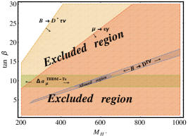
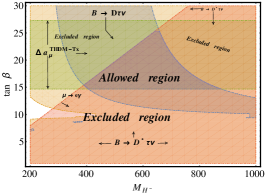
We will now constrain the parameter space for the charged Higgs bosons, following a similar methodology to the one used in the previous section, except that we now consider processes mediated by charged scalars: BD(D)τν𝐵𝐷superscript𝐷𝜏𝜈B\to D(D^{*})\tau\nu, aμTHDMTxsuperscriptsubscript𝑎𝜇𝑇𝐻𝐷𝑀𝑇𝑥a_{\mu}^{THDM-Tx} and μeγ𝜇𝑒𝛾\mu\to e\gamma. The allowed regions for Semi-Parallel and Parallel cases are presented in Figures 11, LABEL:cargados-Paralela. We have performed a thorough analysis of the Complementary case and we found that it was able to satisfy μeγ𝜇𝑒𝛾\mu\to e\gamma, BDτν𝐵superscript𝐷𝜏𝜈B\to D^{*}\tau\nu and ΔaμΔsubscript𝑎𝜇\Delta a_{\mu}, but we where unable to find a region that satisfied BDτν𝐵𝐷𝜏𝜈B\to D\tau\nu and the previous processes. The Complementary case is only able to meet with the limits of neutral Higgs bosons.
Refer to caption
(a)
Refer to caption
(b)
Figure 11: Allowed and excluded regions obtained from the processes mediated by charged Higgs bosons for Semi-Parallel (a) and Parallel (b) cases.

We find that the most restrictive process is BDτν𝐵𝐷𝜏𝜈B\to D\tau\nu. We have used γu=0.13subscript𝛾𝑢0.13\gamma_{u}=0.13, γd=0.1subscript𝛾𝑑0.1\gamma_{d}=0.1 and γl=1subscript𝛾𝑙1\gamma_{l}=1, (αβ)=π2𝛼𝛽𝜋2(\alpha-\beta)=\frac{\pi}{2}, MH0=500subscript𝑀superscript𝐻0500M_{H^{0}}=500 GeV, MA0=300subscript𝑀superscript𝐴0300M_{A^{0}}=300 GeV, Mh0=125subscript𝑀superscript0125M_{h^{0}}=125 GeV α1=α2=0subscript𝛼1subscript𝛼20\alpha_{1}=\alpha_{2}=0, a1u=𝒪(101)superscriptsubscript𝑎1𝑢𝒪superscript101a_{1}^{u}=\mathcal{O}(10^{-1}), a1d=𝒪(103)superscriptsubscript𝑎1𝑑𝒪superscript103a_{1}^{d}=\mathcal{O}(10^{-3}) , a1l=𝒪(103)superscriptsubscript𝑎1𝑙𝒪superscript103a_{1}^{l}=\mathcal{O}(10^{-3}).

V The LHC Signals

In the previous section we determined the allowed parameter space according to current low energy constraints. Now, we will use collider constraints. These need to satisfy the constraint of the SM-like Higgs signal observed at the LHC by including several production and decay Higgs channels. We shall consider only the production of Higgs bosons by gluon fusion and the decays h0ZZsuperscript0𝑍superscript𝑍h^{0}\to ZZ^{*}, γγ𝛾𝛾\gamma\gamma, ττ+superscript𝜏superscript𝜏\tau^{-}\tau^{+}, bb¯𝑏¯𝑏b\bar{b}. Then, in order to reproduce the signal rate for the SM-like Higgs signals with mh125similar-to-or-equalssubscript𝑚125m_{h}\simeq 125 GeV, we consider the following ratios:

RXX=σ(ggh0)σ(gghSM)Br(h0XX)Br(hSMXX),subscript𝑅𝑋𝑋𝜎𝑔𝑔superscript0𝜎𝑔𝑔subscript𝑆𝑀𝐵𝑟superscript0𝑋𝑋𝐵𝑟subscript𝑆𝑀𝑋𝑋R_{XX}=\frac{\sigma(gg\to h^{0})}{\sigma(gg\to h_{SM})}\frac{Br(h^{0}\to XX)}{Br(h_{SM}\to XX)}, (105)

for X=γ,Z,τ,b𝑋𝛾𝑍𝜏𝑏X=\gamma,Z,\tau,b.

Within the so-called narrow-width approximation, we can write the expression for RXXsubscript𝑅𝑋𝑋R_{XX} as follows:

RXX=Γ(h0gg)Γ(hSMgg)Br(h0XX)Br(hSMXX).subscript𝑅𝑋𝑋Γsuperscript0𝑔𝑔Γsubscript𝑆𝑀𝑔𝑔𝐵𝑟superscript0𝑋𝑋𝐵𝑟subscript𝑆𝑀𝑋𝑋R_{XX}=\frac{\Gamma(h^{0}\to gg)}{\Gamma(h_{SM}\to gg)}\,\frac{Br(h^{0}\to XX)}{Br(h_{SM}\to XX)}. (106)

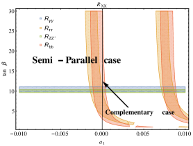
The Higgs signals h0bb¯superscript0𝑏¯𝑏h^{0}\to b\bar{b} and h0ττ+superscript0superscript𝜏superscript𝜏h^{0}\to\tau^{-}\tau^{+} channels have been tested at the LHC due to the relatively large Yukawa couplings. In THDM’s, the bottom and tau Yukawa coupling are expected to be different from those of the SM. The values of the R-parameters according to current LHC Higgs data such as RZZ=1.150.23+0.27subscript𝑅𝑍𝑍subscriptsuperscript1.150.270.23R_{ZZ}=1.15^{+0.27}_{-0.23}, Rγγ=1.170.17+0.19subscript𝑅𝛾𝛾subscriptsuperscript1.170.190.17R_{\gamma\gamma}=1.17^{+0.19}_{-0.17}, Rbb¯=0.85±0.29subscript𝑅𝑏¯𝑏plus-or-minus0.850.29R_{b\bar{b}}=0.85\pm 0.29 and Rτ+τ=0.79±0.26subscript𝑅superscript𝜏superscript𝜏plus-or-minus0.790.26R_{\tau^{+}\tau^{-}}=0.79\pm 0.26 can be found in [30]. Our evaluation of the values of RXXsubscript𝑅𝑋𝑋R_{XX} is done with (αβ)π/2similar-to𝛼𝛽𝜋2(\alpha-\beta)\sim\pi/2, γf=1subscript𝛾𝑓1\gamma_{f}=1, α1subscript𝛼1\alpha_{1}=α2subscript𝛼2\alpha_{2}=0.

The regions that satisfy the constraint for each of the considered channels are presented in Fig. 12,
Refer to caption
Figure 12: Signal strength for RZZsubscript𝑅𝑍superscript𝑍R_{ZZ^{*}}, Rγγsubscript𝑅𝛾𝛾R_{\gamma\gamma}, Rbb¯subscript𝑅𝑏¯𝑏R_{b\bar{b}} and Rττ+subscript𝑅superscript𝜏superscript𝜏R_{\tau^{-}\tau^{+}}.

we find several regions in the tanβmH𝛽subscript𝑚𝐻\tan\beta-m_{H} plane that satisfy the current signal strength measurements.

VI Predictions for h0τμ,tch0formulae-sequencesuperscript0𝜏𝜇𝑡𝑐superscript0h^{0}\to\tau\mu,\;t\to ch^{0}

The decay h0τμsuperscript0𝜏𝜇h^{0}\to\tau\mu provides an interesting signal to probe FV Higgs couplings, it was initially studied in [44, 45]. And subsequent studies on detectability of the signal appeared in [46], while improved calculations within SUSY and other models appeared in [47]; more recent discussions of LFV Higgs decays are presented in [48].

Another interesting signal to probe FV Higgs couplings are rare top decays, particularly tch0𝑡𝑐superscript0t\to ch^{0} which has been studied within the THDM in [49, 50, 51, 52], while the SUSY case was considered in [54, 53]. The search for this mode at LHC was considered in [55].

VI.1 h0τμsuperscript0𝜏𝜇h^{0}\to\tau\mu decay

The first search for the Lepton Flavor Violating (LFV) decay h0τμsuperscript0𝜏𝜇h^{0}\to\tau\mu was performed by CMS [56] and ATLAS [57], at a center of mass energy of 88\sqrt{8} TeV with an integrated luminosity of 19.7fb1𝑓superscript𝑏1fb^{-1}. They reported a slight signal excess with a significance of 2.4σ𝜎\sigma, and give a limit on BR(h0τμsuperscript0𝜏𝜇h^{0}\to\tau\mu)<1.51%absentpercent1.51<1.51\% at 95%percent\% confidence level.

The Feynman diagram at tree level of the h0τμsuperscript0𝜏𝜇h^{0}\to\tau\mu decay is shown in Fig. 13

Refer to caption
Figure 13: Feynman diagram for h0τμsuperscript0𝜏𝜇h^{0}\to\tau\mu decay.
Γ(h0τμ)=g2mμmτ32πMW2|ητμh0|2β3Mh0,Γsuperscript0𝜏𝜇superscript𝑔2subscript𝑚𝜇subscript𝑚𝜏32𝜋superscriptsubscript𝑀𝑊2superscriptsuperscriptsubscript𝜂𝜏𝜇superscript02superscript𝛽3subscript𝑀superscript0\Gamma(h^{0}\to\tau\mu)=\frac{g^{2}m_{\mu}m_{\tau}}{32\pi M_{W}^{2}}\Big{|}\eta_{\tau\mu}^{h^{0}}\Big{|}^{2}\beta^{3}M_{h^{0}}, (107)

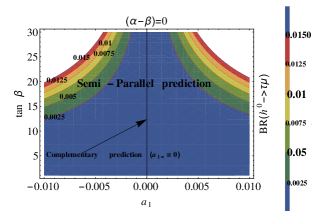
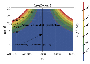
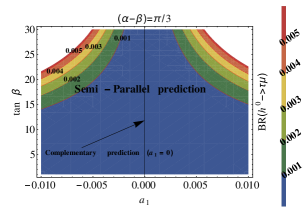
where β=(1(rτh0+rμh0)2)(rτh02rμh021)24rμh02𝛽1superscriptsubscript𝑟𝜏superscript0subscript𝑟𝜇superscript02superscriptsuperscriptsubscript𝑟𝜏superscript02superscriptsubscript𝑟𝜇superscript02124superscriptsubscript𝑟𝜇superscript02\beta=\Big{(}1-{(r_{\tau h^{0}}+r_{\mu h^{0}})^{2}}\Big{)}\sqrt{{(r_{\tau h^{0}}^{2}-r_{\mu h^{0}}^{2}-1)^{2}}-4{r_{\mu h^{0}}^{2}}}, rh0=m/Mh0subscript𝑟superscript0subscript𝑚subscript𝑀superscript0r_{\ell h^{0}}=m_{\ell}/M_{h^{0}}, Mh0subscript𝑀superscript0M_{h^{0}}, mτsubscript𝑚𝜏m_{\tau}, mμsubscript𝑚𝜇m_{\mu} and ητμh0superscriptsubscript𝜂𝜏𝜇superscript0\eta_{\tau\mu}^{h^{0}} are the SM-like Higgs boson, tau and muon masses and h0τμsuperscript0𝜏𝜇h^{0}\tau\mu coupling, respectively. As mentioned previously we have been considering (αβ)=π/2𝛼𝛽𝜋2(\alpha-\beta)=\pi/2 but from eq.68 we identify that this coupling is zero. That is why, we take the limit (αβ)π/2𝛼𝛽𝜋2(\alpha-\beta)\to\pi/2. We also consider the scenarios (αβ)=0𝛼𝛽0(\alpha-\beta)=0, which corresponds to the case where there are no flavor changing neutral currents via a heavy scalar, and (αβ)=π/3𝛼𝛽𝜋3(\alpha-\beta)=\pi/3 which corresponds to an intermediate scenario. In Fig. 14 we show the branching ratios of the decay h0τμsuperscript0𝜏𝜇h^{0}\to\tau\mu for these scenarios as a function of tanβ𝛽\tan\beta and the parameter a1subscript𝑎1a_{1} for the complementary case (a1=0)subscript𝑎10(a_{1}=0) and Semi-Parallel case (0.01a10.01)0.01subscript𝑎10.01(-0.01\leq a_{1}\leq 0.01).

Refer to caption
(a)
Refer to caption
(b)
Figure 14: Branching ratios of the LFV decay h0τμsuperscript0𝜏𝜇h^{0}\to\tau\mu as a function of tanβ𝛽\tan{\beta} and the parameter a1subscript𝑎1a_{1}. The vertical line, whose equation is a1=0subscript𝑎10a_{1}=0, corresponds to the prediction of the complementary case, while the prediction for the Semi-Parallel case is presented in the colored points in the tβsubscript𝑡𝛽t_{\beta}-a1subscript𝑎1a_{1} plane.

The values 0.01a10.010.01subscript𝑎10.01-0.01\leq a_{1}\leq 0.01 are used because this interval satisfies the experimental bounds and values of the process that we considered to restrict the parameter space of our model. Fig. 14(a) corresponds to the (αβ)=0𝛼𝛽0(\alpha-\beta)=0 scenario and Fig. 14(b) corresponds to (αβ)π/2𝛼𝛽𝜋2(\alpha-\beta)\to\pi/2 scenario. We find that this scenario gives the smallest contributions with a BR107similar-to𝐵𝑅superscript107BR\sim 10^{-7}. We only present the branching ratios that fall within the current limit BR(h0τμsuperscript0𝜏𝜇h^{0}\to\tau\mu)<1.51%absentpercent1.51<1.51\% [56]. The graph corresponding to the scenario (αβ)=π/3𝛼𝛽𝜋3(\alpha-\beta)=\pi/3 is shown in appendix B.

VI.2 tch0𝑡𝑐superscript0t\to ch^{0} decay

The Feynman diagram of the tch0𝑡𝑐superscript0t\to ch^{0} decay is shown in Fig. 15,

Refer to caption
Figure 15: Feynman diagram for tch0𝑡𝑐superscript0t\to ch^{0}.

and the decay width is given by

Γ(tch)=mt16π|ηtch0|2[(1+rc)2rht2]×1(rht+rch)21(rhtrhc)2.Γ𝑡𝑐subscript𝑚𝑡16𝜋superscriptsuperscriptsubscript𝜂𝑡𝑐superscript02delimited-[]superscript1subscript𝑟𝑐2superscriptsubscript𝑟𝑡21superscriptsubscript𝑟𝑡subscript𝑟𝑐21superscriptsubscript𝑟𝑡subscript𝑟𝑐2\displaystyle\Gamma(t\to ch)=\frac{m_{t}}{16\pi}\Big{|}\eta_{tc}^{h^{0}}\Big{|}^{2}\Big{[}(1+r_{c})^{2}-r_{ht}^{2}\Big{]}\times\sqrt{1-(r_{ht}+r_{ch})^{2}}\sqrt{1-(r_{ht}-r_{hc})^{2}}. (108)

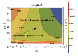
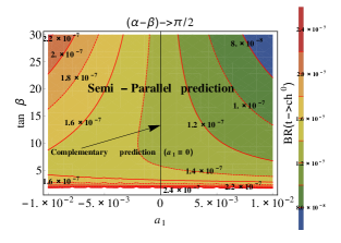
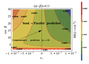
In Fig. 16 we show the Branching ratio of the decay tch0𝑡𝑐superscript0t\to ch^{0} as a function of tanβ𝛽\tan\beta for the complementary case a1=0subscript𝑎10a_{1}=0 and Semi-Parallel case; the values 0.01a10.010.01subscript𝑎10.01-0.01\leq a_{1}\leq 0.01 are used because this interval satisfies the experimental bounds and values of the process that we considered to restrict the parameter space of our model. Fig. 16(a) corresponds to the (αβ)=0𝛼𝛽0(\alpha-\beta)=0 scenario and Fig. 16(b) to (αβ)π/2𝛼𝛽𝜋2(\alpha-\beta)\to\pi/2 scenario. We find that this scenario gives the smallest contributions with a BR107similar-to𝐵𝑅superscript107BR\sim 10^{-7}. We only present the branching ratios that fall within the current limit BR(tch0𝑡𝑐superscript0t\to ch^{0})<5.6×10⁶absent5.6superscript106<5.6\times 10^{-6}

Refer to caption
(a)
Refer to caption
(b)
Figure 16: Branching ratios of the rare decay tch0𝑡𝑐superscript0t\to ch^{0} as a function of tβsubscript𝑡𝛽t_{\beta} and the parameter a1subscript𝑎1a_{1} for (a) (αβ)=0𝛼𝛽0(\alpha-\beta)=0 and (b) (αβ)π/2𝛼𝛽𝜋2(\alpha-\beta)\to\pi/2. The vertical line, whose equation is a1=0subscript𝑎10a_{1}=0, corresponds to the prediction of the complementary case, while the prediction for the Semi-Parallel case is presented in the colored points in the tanβ𝛽\tan{\beta}-a1subscript𝑎1a_{1} plane.

The graph corresponding to the scenario (αβ)=π/3𝛼𝛽𝜋3(\alpha-\beta)=\pi/3 is shown in appendix B.

VII Conclusions

We have considered the possibility that the Yukawa matrices can be constructed in such a way that they produce a specific hermitian mass matrix, which we classify as Semi-Parallel and Complementary textures. This assumption of different matrix textures is relevant in the study of LFV decays and rare quark decays, because the flavor violating couplings for each of these new signals depends on the Yukawa elements Yijsubscript𝑌𝑖𝑗Y_{ij}. Through current experimental bounds from low-energy processes: ΔaμΔsubscript𝑎𝜇\Delta a_{\mu}, KK¯𝐾¯𝐾K-\bar{K} and BB¯𝐵¯𝐵B-\bar{B} mixing, BD(D)τν𝐵𝐷superscript𝐷𝜏𝜈B\rightarrow D(D^{*})\tau\nu, Bs0μ+μsuperscriptsubscript𝐵𝑠0superscript𝜇superscript𝜇B_{s}^{0}\to\mu^{+}\mu^{-}, liljγsubscript𝑙𝑖subscript𝑙𝑗𝛾l_{i}\rightarrow l_{j}\gamma and τμμ+μsuperscript𝜏superscript𝜇superscript𝜇superscript𝜇\tau^{-}\rightarrow\mu^{-}\mu^{+}\mu^{-}, we restrict our parameter space and find that small values of tanβ𝛽\tan\beta and 450MH1000less-than-or-similar-to450subscript𝑀𝐻1000450\lesssim M_{H}\leq 1000 GeV are favored. We then incorporate the LHC Higgs signal strengths Rγγsubscript𝑅𝛾𝛾R_{\gamma\gamma}, RZZsubscript𝑅𝑍superscript𝑍R_{ZZ^{*}}, Rbb¯subscript𝑅𝑏¯𝑏R_{b\bar{b}} and Rττ+subscript𝑅superscript𝜏superscript𝜏R_{\tau^{-}\tau^{+}}. And finally, using all the aforementioned restriction we calculate the branching ratios of the LFV Higgs decay (h0τμsuperscript0𝜏𝜇h^{0}\to\tau\mu), as well as the rare top decay tch0𝑡𝑐superscript0t\to ch^{0}, and we find that the highest contributions are of the order 𝒪(102)𝒪superscript102\mathcal{O}(10^{-2}) and 𝒪(103)𝒪superscript103\mathcal{O}(10^{-3}), for each one. Therefore, our analysis seems to suggests that the case that best satisfies the current experimental bounds and measurements is the Semi-parallel case, while the complementary case offers the simplest pattern of Flavor violating Higgs couplings, as they depend only on a few parameters.

Acknowledgements.
We acknowledge support from CONACYT-SNI (Mexico).

References

  • [1] G. Aad et al. [ATLAS and CMS Collaborations], Phys. Rev. Lett. 114 (2015) 191803 [arXiv:1503.07589].
  • [2] J. F. Gunion, H. E. Haber, G. L. Kane and S. Dawson, Front. Phys.  80, 1 (2000).
  • [3] J. L. Diaz-Cruz and D. A. Lopez-Falcon, Phys. Lett. B 568, 245 (2003) [hep-ph/0304212].
  • [4] N. G. Deshpande and E. Ma, Phys. Rev. D 18, 2574 (1978).
  • [5] S. P. Martin, In *Kane, G.L. (ed.): Perspectives on supersymmetry II* 1-153 [hep-ph/9709356].
  • [6] M. Quiros, hep-ph/0606153.
  • [7] A. Pomarol, CERN Yellow Report CERN-2012-001, 115-151 [arXiv:1202.1391 [hep-ph]].
  • [8] A. Aranda, J. L. Diaz-Cruz, J. Hernandez-Sanchez and R. Noriega-Papaqui, Phys. Lett. B 658, 57 (2007) [arXiv:0708.3821].
  • [9] G. C. Branco, P. M. Ferreira, L. Lavoura, M. N. Rebelo, M. Sher and J. P. Silva, Phys. Rept.  516, 1 (2012) [arXiv:1106.0034].
  • [10] E. Ma, Mod. Phys. Lett. A 21, 1777 (2006) [hep-ph/0605180]. R. Barbieri, L. J. Hall and V. S. Rychkov, Phys. Rev. D 74, 015007 (2006) [hep-ph/0603188]; L. Lopez Honorez, E. Nezri, J. F. Oliver and M. H. G. Tytgat, JCAP 0702, 028 (2007) [hep-ph/0612275]. I. F. Ginzburg, K. A. Kanishev, M. Krawczyk and D. Sokolowska, Phys. Rev. D 82, 123533 (2010) [arXiv:1009.4593].
  • [11] I. F. Ginzburg and M. Krawczyk, Phys. Rev. D 72, 115013 (2005) [hep-ph/0408011].
  • [12] S. L. Glashow and S. Weinberg, Phys. Rev. D 15, 1958 (1977).
  • [13] J. F. Gunion and H. E. Haber, Nucl. Phys. B 307, 445 (1988) [Erratum-ibid. B 402, 569 (1993)].
  • [14] H. Fritzsch and Z. -z. Xing, Phys. Lett. B 353, 114 (1995) [hep-ph/9502297].
  • [15] G. C. Branco, D. Emmanuel-Costa and R. Gonzalez Felipe, Phys. Lett. B 477, 147 (2000) [hep-ph/9911418].
  • [16] L. J. Hall and S. Weinberg, Phys. Rev. D 48, 979 (1993) [hep-ph/9303241].
  • [17] W. Altmannshofer, S. Gori and G. D. Kribs, Phys. Rev. D 86, 115009 (2012) [arXiv:1210.2465].
  • [18] A. J. Buras, M. V. Carlucci, S. Gori and G. Isidori, JHEP 1010, 009 (2010) [arXiv:1005.5310].
  • [19] G. D’Ambrosio, G. F. Giudice, G. Isidori and A. Strumia, Nucl. Phys. B 645, 155 (2002) [hep-ph/0207036].
  • [20] A. Aranda, C. Bonilla and J. L. Diaz-Cruz, Phys. Lett. B 717, 248 (2012) [arXiv:1204.5558].
  • [21] A. Pich and P. Tuzon, Phys. Rev. D 80, 091702 (2009) [arXiv:0908.1554].
  • [22] T. P. Cheng and M. Sher, Phys. Rev. D 35, 3484 (1987).
  • [23] Y. -F. Zhou, J. Phys. G 30, 783 (2004) [hep-ph/0307240].
  • [24] J. L. Diaz-Cruz, R. Noriega-Papaqui and A. Rosado, Phys. Rev.  D 69, 095002 (2004), [hep-ph/0401194].
  • [25] J. L. Diaz-Cruz, R. Noriega-Papaqui and A. Rosado, Phys. Rev. D 71, 015014 (2005) [hep-ph/0410391].
  • [26] Y. -L. Wu and Y. -F. Zhou, Eur. Phys. J. C 36, 89 (2004) [hep-ph/0403252].
  • [27] W. -j. Li, Y. -d. Yang and X. -d. Zhang, Phys. Rev. D 73, 073005 (2006) [hep-ph/0511273].
  • [28] A. E. Carcamo Hernandez, R. Martinez and J. A. Rodriguez, Eur. Phys. J. C 50, 935 (2007) [hep-ph/0606190].
  • [29] D. Atwood, S. Bar-Shalom and A. Soni, Phys. Lett. B 635, 112 (2006) doi:10.1016/j.physletb.2006.02.033 [hep-ph/0502234].
  • [30] K.A. Olive et al. (Particle Data Group), Chin. Phys. C, 38, 090001 (2014) and 2015 update.
  • [31] T. P. Cheng and M. Sher, Phys. Rev. D 35, 3484 (1987).
  • [32] M. Gomez-Bock and R. Noriega-Papaqui, J. Phys. G 32, 761 (2006) [hep-ph/0509353].
  • [33] Dean Carmi, Adam Falkowski, Eric Kuflik, Tomer Volansky, Jure Zupan, 10.1007/JHEP10(2012)196, [arXiv:1207.1718v3].
  • [34] G. Bennett et al. (Muon G-2 Collaboration), Phys.Rev.D73, 072003 (2006), arXiv:hep-ex/0602035.
  • [35] D. Chang, W.-F. Chang, C.-H. Chou, and W.-Y. Keung, Phys.Rev. D 63, 091301(R)(2001).
  • [36] V. Khachatryan et al., [CMS and LHCb Collaborations], [arXiv:1411.4413].
  • [37] C. Bobeth et al. , Phys. Rev. Lett. 112 (2014) 101801.
  • [38] A. Dedes and A. Pilaftsis, Phys. Rev. D 67, 015012 (2003).
  • [39] B. Aubert et al. [BaBar Collaboration], Phys. Rev. D 79, 092002 (2009), [arXiv:0902.2660 [hep-ex]].
  • [40] A. Matyja et al. [Belle Collaboration], Phys. Rev. Lett.  99, 191807 (2007), [arXiv:0706.4429 [hep-ex]].
  • [41] A. Crivellin, C. Greub and A. Kokulu, Phys. Rev. D 86, 054014 (2012), [arXiv:1206.2634 [hep-ph]].
  • [42] J. Adam et al. [MEG Collaboration], Phys. Rev. Lett.  110, no. 20, 201801 (2013) [arXiv:1303.0754].
  • [43] B. Aubert et al. [BaBar Collaboration], Phys. Rev. Lett.  104, 021802 (2010) [arXiv:0908.2381].
  • [44] A. Pilaftsis, Phys. Lett. B 285, 68 (1992).
  • [45] J. L. Diaz-Cruz and J. J. Toscano, Phys. Rev. D 62, 116005 (2000) [hep-ph/9910233].
  • [46] T. Han and D. Marfatia, Phys. Rev. Lett.  86, 1442 (2001) [hep-ph/0008141]; K. A. Assamagan, A. Deandrea and P. -A. Delsart, Phys. Rev. D 67, 035001 (2003) [hep-ph/0207302]; D. McKeen, M. Pospelov and A. Ritz, Phys. Rev. D 86, 113004 (2012) [arXiv:1208.4597].
  • [47] J. L. Diaz-Cruz, JHEP 0305, 036 (2003) [hep-ph/0207030]; A. Brignole and A. Rossi, Nucl. Phys. B 701, 3 (2004) [hep-ph/0404211]. E. Arganda, A. M. Curiel, M. J. Herrero and D. Temes, Phys. Rev. D 71, 035011 (2005) [hep-ph/0407302]. S. Kanemura, T. Ota and K. Tsumura, Phys. Rev. D 73, 016006 (2006) [hep-ph/0505191].
  • [48] J. L. Diaz-Cruz, D. K. Ghosh and S. Moretti, Phys. Lett. B 679, 376 (2009) [arXiv:0809.5158]. M. Arana-Catania, E. Arganda and M. J. Herrero, [arXiv:1304.3371]; A. Arhrib, Y. Cheng and O. C. W. Kong, Phys. Rev. D 87, 015025 (2013) [arXiv:1210.8241]; R. Harnik, J. Kopp and J. Zupan, JHEP 1303, 026 (2013) [arXiv:1209.1397]. A. Goudelis, O. Lebedev and J. -h. Park, Phys. Lett. B 707, 369 (2012) [arXiv:1111.1715].
  • [49] G. Eilam, J. L. Hewett and A. Soni, Phys. Rev. D 44, 1473 (1991) [Erratum-ibid. D 59, 039901 (1999)].
  • [50] B. Mele, S. Petrarca and A. Soddu, Phys. Lett. B 435, 401 (1998) [hep-ph/9805498].
  • [51] S. Bejar, J. Guasch and J. Sola, hep-ph/0101294.
  • [52] B. Mele, hep-ph/0003064.
  • [53] J. L. Diaz-Cruz, R. Martinez, M. A. Perez and A. Rosado, Phys. Rev. D 41, 891 (1990).
  • [54] J. L. Diaz-Cruz, H. -J. He and C. P. Yuan, Phys. Lett. B 530, 179 (2002) [hep-ph/0103178].
  • [55] J. A. Aguilar-Saavedra and G. C. Branco, Phys. Lett. B 495, 347 (2000) [hep-ph/0004190].
  • [56] V. Khachatryan et al. [CMS Collaboration], arXiv:1502.07400.
  • [57] Aad, Georges, et. al., [ATLAS Collaboration], arXiv:1604.07730.

Appendix A Yukawa matrices: Cases 2-6 .

Case 2:

Y1=(0d0dc0000),Y2=(00000b0ba).formulae-sequencesubscript𝑌10𝑑0superscript𝑑𝑐0000subscript𝑌200000𝑏0superscript𝑏𝑎{Y}_{1}=\left(\begin{array}[]{ccc}0&d&0\\ d^{*}&c&0\\ 0&0&0\end{array}\right),{Y}_{2}=\left(\begin{array}[]{ccc}0&0&0\\ 0&0&b\\ 0&b^{*}&a\end{array}\right).

Case 3:

Y1=(0d0d0b0b0),Y2=(0000c000a).formulae-sequencesubscript𝑌10𝑑0superscript𝑑0𝑏0superscript𝑏0subscript𝑌20000𝑐000𝑎{Y}_{1}=\left(\begin{array}[]{ccc}0&d&0\\ d^{*}&0&b\\ 0&b^{*}&0\end{array}\right),{Y}_{2}=\left(\begin{array}[]{ccc}0&0&0\\ 0&c&0\\ 0&0&a\end{array}\right).

Case 4:

Y1=(0000cb0b0),Y2=(0d0d0000a).formulae-sequencesubscript𝑌10000𝑐𝑏0superscript𝑏0subscript𝑌20𝑑0superscript𝑑0000𝑎{Y}_{1}=\left(\begin{array}[]{ccc}0&0&0\\ 0&c&b\\ 0&b^{*}&0\end{array}\right),{Y}_{2}=\left(\begin{array}[]{ccc}0&d&0\\ d^{*}&0&0\\ 0&0&a\end{array}\right).

Case 5:

Y1=(00000b0b0),Y2=(0d0dc000a).formulae-sequencesubscript𝑌100000𝑏0superscript𝑏0subscript𝑌20𝑑0superscript𝑑𝑐000𝑎{Y}_{1}=\left(\begin{array}[]{ccc}0&0&0\\ 0&0&b\\ 0&b^{*}&0\end{array}\right),{Y}_{2}=\left(\begin{array}[]{ccc}0&d&0\\ d^{*}&c&0\\ 0&0&a\end{array}\right).

Case 6:

Y1=(0d0d00000),Y2=(0000cb0ba).formulae-sequencesubscript𝑌10𝑑0superscript𝑑00000subscript𝑌20000𝑐𝑏0superscript𝑏𝑎{Y}_{1}=\left(\begin{array}[]{ccc}0&d&0\\ d^{*}&0&0\\ 0&0&0\end{array}\right),{Y}_{2}=\left(\begin{array}[]{ccc}0&0&0\\ 0&c&b\\ 0&b^{*}&a\end{array}\right).

Case 7:

Y1=(0000c0000),Y2=(0d0d0b0ba).formulae-sequencesubscript𝑌10000𝑐0000subscript𝑌20𝑑0superscript𝑑0𝑏0superscript𝑏𝑎{Y}_{1}=\left(\begin{array}[]{ccc}0&0&0\\ 0&c&0\\ 0&0&0\end{array}\right),{Y}_{2}=\left(\begin{array}[]{ccc}0&d&0\\ d^{*}&0&b\\ 0&b^{*}&a\end{array}\right).

Appendix B Scenario (αβ)=π/3𝛼𝛽𝜋3(\alpha-\beta)=\pi/3 .

Refer to caption
(a)
Refer to caption
(b)
Figure 17: (a) Branching ratios of the LFV decay h0τμsuperscript0𝜏𝜇h^{0}\to\tau\mu as a function of tβsubscript𝑡𝛽t_{\beta} for the scenario (αβ)=π3𝛼𝛽𝜋3(\alpha-\beta)=\frac{\pi}{3}. (b) Branching ratios of the rare top decay tch0𝑡𝑐superscript0t\to ch^{0} for the scenario (αβ)=π3𝛼𝛽𝜋3(\alpha-\beta)=\frac{\pi}{3}.