Preprint No: NSF-KITP-13-080.

Radiative Decays of Cosmic Background Neutrinos in Extensions of MSSM with a Vector Like Lepton Generation

Amin Aboubrahim^b, Tarek Ibrahim^a,b and Pran Nath^c,d

a. Department of Physics, Faculty of Science, University of Alexandria,
Alexandria 21511, Egypt
b. Department of Physics, Faculty of Sciences, Beirut Arab University, Beirut 11 - 5020, Lebanon
c. Department of Physics, Northeastern University, Boston, MA 02115-5000, USA
d. KITP, University of California, Santa Barbara, CA 93106-4030

Abstract

An analysis of radiative decays of the neutrinos $\nu_{j}\to\nu_{l}\gamma$ is discussed in MSSM extensions with a vector like lepton generation. Specifically we compute neutrino decays arising from the exchange of charginos and charged sleptons where the photon is emitted by the charged particle in the loop. It is shown that while the lifetime of the neutrino decay in the Standard Model is $\sim 10^{43}$ yrs for a neutrino mass of 50 meV, the current lower limit from experiment from the analysis of the Cosmic Infrared Background is $\sim 10^{12}$ yrs and thus beyond the reach of experiment in the foreseeable future. However, in the extensions with a vector like lepton generation the lifetime for the decays can be as low as $\sim 10^{12}-10^{14}$ yrs and thus within reach of future improved experiments. The effect of CP phases on the neutrino lifetime is also analyzed. It is shown that while both the magnetic and the electric transition dipole moments contribute to the neutrino lifetime, often the electric dipole moment dominates even for moderate size CP phases.

Keywords:  Cosmic background neutrinos, radiative neutrino decay, vector lepton multiplets
PACS numbers: 13.40Em, 12.60.-i, 14.60.Fg

1 Introduction

It is well known that a neutrino can decay radiatively to neutrinos with lower masses. Thus for the neutrino mass eigenstates $\nu_{1}$, $\nu_{2}$, $\nu_{3}$, with $m_{\nu_{3}}>m_{\nu_{2}}>m_{\nu_{1}}$ one can have radiative decays so that $\nu_{3}\to\nu_{1}\gamma,\nu_{2}\gamma$. In the Standard Model this process can proceed by the exchange of a charged lepton and a W boson so that $\nu_{3}\to l^{-}W^{+}(loop)\to\nu_{1,2}\gamma$. However, the lifetime for the neutrino decay in the Standard Model is rather large [1], i.e.,

$$\tau_{\nu_{3}}^{SM}\sim 10^{43}~{}~{}{\rm yrs},$$ (1)

for a $\nu_{3}$ with mass 50 meV. Now the current lower limit based on data from galaxy surveys with infrared satellites AKARI [2], Spitzer [3] and Hershel [4] as well as the high precision cosmic microwave background (CMB) data collected by the Far Infrared Absolute Spectrometer (FIRAS) on board the Cosmic Background explorer (COBE) [5] for the study of radiative decays of the cosmic neutrinos[6] using the Cosmic Infrared Background (CIB) gives [6]

$$\tau_{\nu_{3}}^{exp}\geq 10^{12}~{}~{}{\rm yrs}$$ (2)

This lower limit is below the Standard Model prediction of Eq.(1) by over 30 orders of magnitude and thus the study of cosmic neutrinos using the Cosmic Infrared Background is unlikely to be fruitful in testing the radiative decays of the neutrinos in the Standard Model. However, much lower lifetimes for the neutrino decays can be achieved when one goes beyond the Standard Model. For example, radiative decays of the neutrinos have been discussed in extensions of the standard model with a heavy mirror generation [7]. Using their result one finds a neutrino lifetime $\sim 10^{20}$ yrs which while much smaller than the one given by the Standard Model is still eight orders of magnitude above the current level of sensitivity. Similarly in the left-right symmetric models, calculations show that one can lower the lifetime for the decay of the neutrino significantly so that [6] $\tau_{\nu_{3}}^{LR}\sim 1.5\times 10^{17}~{}~{}{\rm yrs}$. The experimental measurement using radiative decays provides a way to measure the absolute mass of the neutrino. Thus consider the decay $\nu_{j}\to\nu_{l}\gamma$. In the rest frame of the decay of $\nu_{j}$ the photon energy is given by $E_{\gamma}=(m_{j}^{2}-m_{l}^{2})/(2m_{j})$. Since neutrino oscillations provide us with the neutrino mass difference $m_{j}^{2}-m_{l}^{2}$, a measurement of the photon energy allows a determination of $m_{j}$. Thus the study of Cosmic Infrared Background provides us with an alternative way to fix the absolute value of the neutrino mass aside from the neutrino less double beta decay.

In this work we will discuss a new class of models where the neutrino lifetimes as low as close to the current experimental lower limits can be obtained which makes the study of the lifetimes of the cosmic neutrinos using CIB interesting. Specifically we consider neutrino decay via a light vector like generation. Light vector like generations have been discussed in a variety of works recently. Specifically these include the neutrino magnetic moments [8], contribution to EDMs of leptons [9] and quarks EDMs [10, 11], contribution to radiative decay of charged leptons [12] and to variety of other phenomena [13, 14, 15, 16, 17]. Like the flavor changing radiative decay of the charged leptons (for a review see [18] ) the radiative decays of the neutrinos provide a window to new physics. With the inclusion of the vector generation we also expect the radiative decays of the neutrinos could be significantly larger than in the Standard Model. The reason for this expectation is the following: In the analysis of the decay $\tau\to\mu\gamma$ it is found [12] that the decay for this process is much larger in models with vector like multiplets than in conventional models. We expect that a similar phenomenon will occur in the analysis of the radiative decay of the neutrinos. This is so because the diagrams that enter in the neutrino radiative decay are very similar to the diagrams that enter in the analysis of the radiative decay of the $\tau$. Thus we expect that the analysis would yield a decay lifetime which would be orders of magnitude closer to the current experimental limits than the result from the Standard Model. In the analysis we will impose the most recent constraints from the Planck satellite experiment [19], i.e., that $\sum_{i}m_{\nu_{i}}<0.85{\rm~{}eV}~{}(95\%~{}CL)$ as well as the neutrino oscillation constraints [20] on the mass differences $\Delta m^{2}_{31}\equiv m_{3}^{2}-m_{1}^{2}=2.4^{+0.12}_{-0.11}\times 10^{-3}$eV², and $\Delta m_{21}^{2}\equiv m_{2}^{2}-m_{1}^{2}=7.65^{+0.23}_{-0.20}\times 10^{-5}$eV².

We note in passing that the radiative decays of the cosmic neutrinos in a supersymmetric framework was discussed in early work in [21]. However, in their work the radiative decay of neutrinos with testable lifetimes make flavor changing processes in the charged lepton sector exceed the experimental limits. Thus these authors had to consider broken R parity models to circumvent these constraints. In our work there are no problems of this sort in the analysis presented here. Indeed the flavor changing neutral currents in the charged sector were already discussed in this class of models in  [12] and the results are consistent with current limits with the possibility of detection of such processes in improved experiment. The reason why the flavor changing neutral current processes in the charged sector do not constrain the radiative decays of the neutrinos is because while the couplings $f_{4},f_{4}^{\prime},f_{4}^{\prime\prime}$ in Eq.(6) enter the charged lepton sector, they do not enter the neutrino sector. Further, while the couplings $f_{5},f_{5}^{\prime},f_{5}^{\prime\prime}$ enter the neutrino sector they do not enter the charged lepton sector. This allows one to suppress the neutral current processes in the charged lepton sector without a problem. In a similar fashion the muon g-2 experiment does not put any constraint on the current analysis. This is so because the contribution of the vector-like multiplet to $g_{\mu}-2$ would arise from couplings $f_{4},f_{4}^{\prime},f_{4}^{\prime\prime}$ which as already indicated above do not enter in the radiative decays of the neutrinos and these couplings can be adjusted so that the contribution of the vector like multiplet to $g_{\mu}-2$ is consistent with the current $g_{\mu}-2$ limits. We have not done an explicit analysis of it here since these couplings do not enter in the radiative decays of the neutrinos and hence are not relevant for the analysis of this paper.

2 Extension of MSSM with a vector multiplet

Vector like multiplets arise in a variety of unified models [22] some of which could be low lying. Here we simply assume the existence of one low lying leptonic vector multiplet which is anomaly free in addition to the MSSM spectrum. Before proceeding further it is useful to record the quantum numbers of the leptonic matter content of this extended MSSM spectrum under $SU(3)_{C}\times SU(2)_{L}\times U(1)_{Y}$. Thus under $SU(3)_{C}\times SU(2)_{L}\times U(1)_{Y}$ the leptons of the three generations transform as follows

$$\psi_{iL}\equiv\left(\matrix{\nu_{iL}\cr~{}{l}_{iL}}\right)\sim(1,2,-\frac{1}{2}),l^{c}_{iL}\sim(1,1,1),~{}\nu^{c}_{iL}\sim(1,1,0),~{}i=1,2,3$$ (3)

where the last entry on the right hand side of each $\sim$ is the value of the hypercharge $Y$ defined so that $Q=T_{3}+Y$. These leptons have $V-A$ interactions. We can now add a vector like multiplet where we have a fourth family of leptons with $V-A$ interactions whose transformations can be gotten from Eq.(3) by letting i run from 1-4. A vector like lepton multiplet also has mirrors and so we consider these mirror leptons which have $V+A$ interactions. Their quantum numbers are as follows

$$\chi^{c}\equiv\left(\matrix{E_{L}^{c}\cr N_{L}^{c}}\right)\sim(1,2,\frac{1}{2}),E_{L}\sim(1,1,-1),N_{L}\sim(1,1,0).$$ (4)

The MSSM Higgs doublets as usual have the quantum numbers

$$H_{1}\equiv\left(\matrix{H_{1}^{1}\cr H_{1}^{2}}\right)\sim(1,2,-\frac{1}{2}),~{}H_{2}\equiv\left(\matrix{H_{2}^{1}\cr H_{2}^{2}}\right)\sim(1,2,\frac{1}{2}).$$ (5)

As mentioned already we assume that the vector multiplet escapes acquiring mass at the GUT scale and remains light down to the electroweak scale. As in the analysis of Ref.[9] interesting new physics arises when we consider the mixing of the second and third generations of leptons with the mirrors of the vector like multiplet. Actually we will extend our model to include the mixing of the first generation as well, for the computation of the decay $\nu_{3}\to\nu_{2,1}\gamma$. Thus the superpotential of the model may be written in the form

$$W=-\mu\epsilon_{ij}\hat{H}_{1}^{i}\hat{H}_{2}^{j}+\epsilon_{ij}[f_{1}\hat{H}_{1}^{i}\hat{\psi}_{L}^{j}\hat{\tau}^{c}_{L}+f_{1}^{\prime}\hat{H}_{2}^{j}\hat{\psi}_{L}^{i}\hat{\nu}^{c}_{\tau L}+f_{2}\hat{H}_{1}^{i}\hat{\chi}^{c}{{}^{j}}\hat{N}_{L}+f_{2}^{\prime}H_{2}^{j}\hat{\chi}^{c}{{}^{i}}\hat{E}_{L}$$

$$+h_{1}H_{1}^{i}\hat{\psi}_{\mu L}^{j}\hat{\mu}^{c}_{L}+h_{1}^{\prime}H_{2}^{j}\hat{\psi}_{\mu L}^{i}\hat{\nu}^{c}_{\mu L}+h_{2}H_{1}^{i}\hat{\psi}_{eL}^{j}\hat{e}^{c}_{L}+h_{2}^{\prime}H_{2}^{j}\hat{\psi}_{eL}^{i}\hat{\nu}^{c}_{eL}]$$

$$+f_{3}\epsilon_{ij}\hat{\chi}^{c}{{}^{i}}\hat{\psi}_{L}^{j}+f_{3}^{\prime}\epsilon_{ij}\hat{\chi}^{c}{{}^{i}}\hat{\psi}_{\mu L}^{j}$$

$$+f_{4}\hat{\tau}^{c}_{L}\hat{E}_{L}+f_{5}\hat{\nu}^{c}_{\tau L}\hat{N}_{L}+f_{4}^{\prime}\hat{\mu}^{c}_{L}\hat{E}_{L}+f_{5}^{\prime}\hat{\nu}^{c}_{\mu L}\hat{N}_{L}$$

$$+f_{3}^{\prime\prime}\epsilon_{ij}\hat{\chi}^{c}{{}^{i}}\hat{\psi}_{eL}^{j}+f_{4}^{\prime\prime}\hat{e}^{c}_{L}\hat{E}_{L}+f_{5}^{\prime\prime}\hat{\nu}^{c}_{eL}\hat{N}_{L}$$ (6)

where $\hat{\psi}_{L}$ stands for $\hat{\psi}_{3L}$, $\hat{\psi}_{\mu L}$ stands for $\hat{\psi}_{2L}$ and $\hat{\psi}_{eL}$ stands for $\hat{\psi}_{1L}$. Here we assume a mixing between the mirror generation and the third lepton generation through the couplings $f_{3}$, $f_{4}$ and $f_{5}$. We also assume mixing between the mirror generation and the second lepton generation through the couplings $f_{3}^{\prime}$, $f_{4}^{\prime}$ and $f_{5}^{\prime}$. The same is true for the mixing between the mirror generation and the first lepton generation through the couplings $f_{3}^{\prime\prime}$, $f_{4}^{\prime\prime}$ and $f_{5}^{\prime\prime}$. The above nine mass terms are responsible for generating lepton flavor changing process. We will focus here on the supersymmetric sector. Then through the terms $f_{3},f_{4},f_{5},f_{3}^{\prime},f_{4}^{\prime},f_{5}^{\prime},f_{3}^{\prime\prime},f_{4}^{\prime\prime},f_{5}^{\prime\prime}$ one can have a mixing between the third generation, the second and the first generation leptons which allows the decay of $\nu_{3}\to\nu_{2,1}\gamma$ through loop corrections that include charginos and scalar lepton exchanges with the photon being emitted by the chargino or by a charged slepton. The mass terms for the leptons and mirrors arise from the term

$${\cal{L}}=-\frac{1}{2}\frac{\partial^{2}W}{\partial{A_{i}}\partial{A_{j}}}\psi_{i}\psi_{j}+H.c.$$ (7)

where $\psi$ and $A$ stand for generic two-component fermion and scalar fields. After spontaneous breaking of the electroweak symmetry, ($\langle H_{1}^{1}\rangle=v_{1}/\sqrt{2}$ and $\langle H_{2}^{2}\rangle=v_{2}/\sqrt{2}$), we have the following set of mass terms written in the 4-component spinor notation

$$-{\cal L}_{m}=\left(\matrix{\bar{\nu}_{\tau R}&\bar{N}_{R}&\bar{\nu}_{\mu R}&\bar{\nu}_{eR}}\right)\left(\matrix{f^{\prime}_{1}v_{2}/\sqrt{2}&f_{5}&0&0\cr-f_{3}&f_{2}v_{1}/\sqrt{2}&-f_{3}^{\prime}&-f_{3}^{\prime\prime}\cr 0&f_{5}^{\prime}&h_{1}^{\prime}v_{2}/\sqrt{2}&0\cr 0&f_{5}^{\prime\prime}&0&h_{2}^{\prime}v_{2}/\sqrt{2}}\right)\left(\matrix{\nu_{\tau L}\cr N_{L}\cr\nu_{\mu L}\cr\nu_{eL}}\right)+H.c.$$ (8)

Here the mass matrices are not Hermitian and one needs to use bi-unitary transformations to diagonalize them. Thus we write the linear transformations

$$\left(\matrix{\nu_{\tau_{R}}\cr N_{R}\cr\nu_{\mu_{R}}\cr\nu_{e_{R}}}\right)=D^{\nu}_{R}\left(\matrix{\psi_{1_{R}}\cr\psi_{2_{R}}\cr\psi_{3_{R}}\cr\psi_{4_{R}}}\right),$$

$$\left(\matrix{\nu_{\tau_{L}}\cr N_{L}\cr\nu_{\mu_{L}}\cr\nu_{e_{L}}}\right)=D^{\nu}_{L}\left(\matrix{\psi_{1_{L}}\cr\psi_{2_{L}}\cr\psi_{3_{L}}\cr\psi_{4_{L}}}\right),$$ (9)

such that

$$D^{\nu\dagger}_{R}\left(\matrix{f^{\prime}_{1}v_{2}/\sqrt{2}&f_{5}&0&0\cr-f_{3}&f_{2}v_{1}/\sqrt{2}&-f_{3}^{\prime}&-f_{3}^{\prime\prime}\cr 0&f_{5}^{\prime}&h_{1}^{\prime}v_{2}/\sqrt{2}&0\cr 0&f_{5}^{\prime\prime}&0&h_{2}^{\prime}v_{2}/\sqrt{2}}\right)D^{\nu}_{L}=diag(m_{\psi_{1}},m_{\psi_{2}},m_{\psi_{3}},m_{\psi_{4}}).$$ (10)

In Eq.(10) $\psi_{1},\psi_{2},\psi_{3},\psi_{4}$ are the mass eigenstates for the neutrinos, where in the limit of no mixing we identify $\psi_{1}$ as the light tau neutrino, $\psi_{2}$ as the heavier mass eigen state, $\psi_{3}$ as the muon neutrino and $\psi_{4}$ as the electron neutrino. To make contact with the normal neutrino hierarchy we relabel the states so that

$$\nu_{1}=\psi_{4},\nu_{2}=\psi_{3},\nu_{3}=\psi_{1},\nu_{4}=\psi_{2}$$ (11)

which we assume has the mass hierarchical pattern

$$m_{\nu_{1}}<m_{\nu_{2}}<m_{\nu_{3}}<m_{\nu_{4}}$$ (12)

We will carry out the analytical analysis in the $\psi_{i}$ notation but the numerical analysis will be carried out in the $\nu_{i}$ notation to make direct contact with data. Next we consider the mixing of the charged sleptons and the charged mirror sleptons. The mass squared matrix of the slepton - mirror slepton comes from three sources, the F term, the D term of the potential and the soft susy breaking terms. Using the superpotential of Eq.(6) the mass terms arising from it after the breaking of the electroweak symmetry are given by the Lagrangian

$${\cal L}={\cal L}_{F}+{\cal L}_{D}$$ (13)

where ${\cal L}_{F}$ and ${\cal L}_{D}$ are given in the Appendix along with the matrix elements of the slepton mass squared matrix.

3 Interactions of charginos, sleptons and neutrinos

The chargino exchange contribution to the decay of the tau neutrino into a muon neutrino (electron neutrino) and a photon arises through the loop diagram in Fig.(1). The relevant part of the Lagrangian that generates this contribution is given by

$$-{\cal{L}}_{\nu-\tilde{\tau}-\chi^{+}}=\sum_{j=1}^{4}\sum_{i=1}^{2}\sum_{k=1}^{8}\bar{\psi}_{j}[C^{L}_{jik}P_{L}+C^{R}_{jik}P_{R}]\tilde{\chi}^{+}_{i}\tilde{\tau}_{k}+H.c.$$ (14)

where

$$C^{L}_{jik}=-f^{\prime}_{1}V^{*}_{i2}D^{\nu*}_{R_{1j}}\tilde{D}^{\tau}_{1k}-f^{\prime}_{2}V^{*}_{i2}D^{\nu*}_{R_{2j}}\tilde{D}^{\tau}_{2k}$$

$$+gV^{*}_{i1}D^{\nu*}_{R_{2j}}\tilde{D}^{\tau}_{4k}-h^{\prime}_{1}V^{*}_{i2}D^{\nu*}_{R_{3j}}\tilde{D}^{\tau}_{5k}-h^{\prime}_{2}V^{*}_{i2}D^{\nu*}_{R_{4j}}\tilde{D}^{\tau}_{7k},$$

$$C^{R}_{jik}=-f_{1}U_{i2}D^{\nu*}_{L_{1j}}\tilde{D}^{\tau}_{3k}-h_{1}U_{i2}D^{\nu*}_{L_{3j}}\tilde{D}^{\tau}_{6k}+gU_{i1}D^{\nu*}_{L_{1j}}\tilde{D}^{\tau}_{1k}$$

$$+gU_{i1}D^{\nu*}_{L_{4j}}\tilde{D}^{\tau}_{7k}-h_{2}U_{i2}D^{\nu*}_{L_{4j}}\tilde{D}^{\tau}_{8k}-f_{2}U_{i2}D^{\nu*}_{L_{2j}}\tilde{D}^{\tau}_{4k},$$ (15)

where $\tilde{D}^{\tau}$ is the diagonalizing matrix of the scalar $8\times 8$ mass squared matrix for the scalar leptons as defined in the Appendix. In Eq.(15) $U$ and $V$ are the matrices that diagonalize the chargino mass matrix $M_{C}$ so that

$$U^{*}M_{C}V^{-1}=diag(m_{\tilde{\chi_{1}}}^{+},m_{\tilde{\chi_{2}}}^{+}).$$ (16)

Figure 1: The diagrams that allow decay of the $\psi_{j}$ into $\psi_{l}+\gamma$ via supersymmetric loops involving the charginos and the staus where the photon is either emitted by the chargino (left) or by the stau (right) inside the loop.

4 The analysis of $\psi_{j}\rightarrow\psi_{l}+\gamma$ decay width

The decay $\psi_{j}\rightarrow\psi_{l}+\gamma$ is induced by one-loop electric and magnetic transition dipole moments, which arise from the diagrams of Fig.(1). In the dipole moment loop, the incoming $\psi_{j}$ is replaced by a $\psi_{l}$. For an incoming $\psi_{j}$ of momentum $p$ and a resulting $\psi_{l}$ of momentum $p^{\prime}$, we define the amplitude

$$\langle\psi_{l}(p^{\prime})|J_{\alpha}|\psi_{j}(p)\rangle=\bar{u}_{\psi_{l}}(p^{\prime})\Gamma_{\alpha}u_{\psi_{j}}(p)$$ (17)

where

$$\Gamma_{\alpha}(q)=\frac{F^{jl}_{2}(q)i\sigma_{\alpha\beta}q^{\beta}}{m_{\psi_{j}}+m_{\psi_{l}}}+\frac{F^{jl}_{3}(q)\sigma_{\alpha\beta}\gamma_{5}q^{\beta}}{m_{\psi_{j}}+m_{\psi_{l}}}+.....$$ (18)

with $q=p-p^{\prime}$ and where $m_{f}$ denotes the mass of the fermion $f$. The decay width of $\psi_{j}\rightarrow\psi_{l}+\gamma$ is given by

$$\Gamma(\psi_{j}\rightarrow\psi_{l}+\gamma)=\frac{m^{3}_{\psi_{j}}}{8\pi(m_{\psi_{j}}+m_{\psi_{l}})^{2}}\left(1-\frac{m^{2}_{\psi_{l}}}{m^{2}_{\psi_{j}}}\right)^{3}\{|F^{jl}_{2}(0)|^{2}+|F^{jl}_{3}(0)|^{2}\}$$ (19)

where the form factors $F^{jl}_{2}$ and $F^{jl}_{3}$ arise from the left and the right loops of Fig. (1) as follows

$$F^{jl}_{2}(0)=F^{jl}_{2~{}left}+F^{jl}_{2~{}right}$$

$$F^{jl}_{3}(0)=F^{jl}_{3~{}left}+F^{jl}_{3~{}right}$$ (20)

The chargino contribution $F^{jl}_{2~{}left}$ is given by

$$F^{jl}_{2~{}left}=-\sum_{i=1}^{2}\sum_{k=1}^{8}\Bigg{[}\frac{(m_{\psi_{j}}+m_{\psi_{l}})}{64\pi^{2}m_{\tilde{\chi_{i}}^{+}}}\{C^{L}_{lik}C^{R*}_{jik}+C^{R}_{lik}C^{L*}_{jik}\}F_{3}\left(\frac{M^{2}_{\tilde{\tau_{k}}}}{m^{2}_{\tilde{\chi_{i}}^{+}}}\right)$$

$$+\frac{m_{\psi_{j}}(m_{\psi_{j}}+m_{\psi_{l}})}{192\pi^{2}m^{2}_{\tilde{\chi_{i}}^{+}}}\{C^{L}_{lik}C^{L*}_{jik}+C^{R}_{lik}C^{R*}_{jik}\}F_{4}\left(\frac{M^{2}_{\tilde{\tau_{k}}}}{m^{2}_{\tilde{\chi_{i}}^{+}}}\right)\Bigg{]}$$ (21)

where

$$F_{3}(x)=\frac{1}{(x-1)^{3}}\{3x^{2}-4x+1-2x^{2}\ln x\}$$ (22)

and

$$F_{4}(x)=\frac{1}{(x-1)^{4}}\{2x^{3}+3x^{2}-6x+1-6x^{2}\ln x\}$$ (23)

The right contribution $F^{jl}_{2~{}right}$ is given by

$$F^{jl}_{2~{}right}=\sum_{i=1}^{2}\sum_{k=1}^{8}\Bigg{[}\frac{(m_{\psi_{j}}+m_{\psi_{l}})}{64\pi^{2}m_{\tilde{\chi_{i}}^{+}}}\{C^{L}_{lik}C^{R*}_{jik}+C^{R}_{lik}C^{L*}_{jik}\}F_{1}\left(\frac{M^{2}_{\tilde{\tau_{k}}}}{m^{2}_{\tilde{\chi_{i}}^{+}}}\right)$$

$$+\frac{m_{\psi_{j}}(m_{\psi_{j}}+m_{\psi_{l}})}{192\pi^{2}m^{2}_{\tilde{\chi_{i}}^{+}}}\{C^{L}_{lik}C^{L*}_{jik}+C^{R}_{lik}C^{R*}_{jik}\}F_{2}\left(\frac{M^{2}_{\tilde{\tau_{k}}}}{m^{2}_{\tilde{\chi_{i}}^{+}}}\right)\Bigg{]}$$ (24)

where

$$F_{1}(x)=\frac{1}{(x-1)^{3}}\{1-x^{2}+2x\ln x\}$$ (25)

and

$$F_{2}(x)=\frac{1}{(x-1)^{4}}\{-x^{3}+6x^{2}-3x-2-6x\ln x\}$$ (26)

The left contribution $F^{jl}_{3~{}left}$ is given by

$$F^{jl}_{3~{}left}=-\sum_{i=1}^{2}\sum_{k=1}^{8}\frac{(m_{\psi_{j}}+m_{\psi_{l}})m_{\tilde{\chi_{i}}^{+}}}{32\pi^{2}M^{2}_{\tilde{\tau_{k}}}}\{C^{L}_{jik}C^{R*}_{lik}-C^{R}_{jik}C^{L*}_{lik}\}F_{6}\left(\frac{m^{2}_{\tilde{\chi_{i}}^{+}}}{M^{2}_{\tilde{\tau_{k}}}}\right)$$ (27)

where

$$F_{6}(x)=\frac{1}{2(x-1)^{2}}\Bigg{\{}-x+3+\frac{2\ln x}{1-x}\Bigg{\}}$$ (28)

The right contribution $F^{jl}_{3~{}right}$ is given by

$$F^{jl}_{3~{}right}=\sum_{i=1}^{2}\sum_{k=1}^{8}\frac{(m_{\psi_{j}}+m_{\psi_{l}})m_{\tilde{\chi_{i}}^{+}}}{32\pi^{2}M^{2}_{\tilde{\tau_{k}}}}\{C^{L}_{jik}C^{R*}_{lik}-C^{R}_{jik}C^{L*}_{lik}\}F_{5}\left(\frac{m^{2}_{\tilde{\chi_{i}}^{+}}}{M^{2}_{\tilde{\tau_{k}}}}\right)$$ (29)

where

$$F_{5}(x)=\frac{1}{2(x-1)^{2}}\Bigg{\{}1+x+\frac{2x\ln x}{1-x}\Bigg{\}}$$ (30)

Now for the numerical analysis below we switch from the $\psi_{i}$ notation to the $\nu_{i}$ notation. Here $\nu_{1},\nu_{2},\nu_{3}$ are the three neutrino mass eigenstates and we assume the mass hierarchy so that $\nu_{3}$ is heavier than $\nu_{2}$ and $\nu_{2}$ is heavier than $\nu_{1}$. For the cosmic neutrinos we are interested in the decay of the $\nu_{3}$ to $\nu_{2}$ and $\nu_{1}$. Thus the total decay width of $\nu_{3}$ is given by $\Gamma_{total}(\nu_{3})=\Gamma(\nu_{3}\rightarrow\nu_{2}+\gamma)+\Gamma(\nu_{3}\rightarrow\nu_{1}+\gamma)$. The lifetime of the tau neutrino is calculated from the equation

$$\tau(\nu_{3})=\frac{\hbar}{\Gamma_{total}(\nu_{3})}$$ (31)

where the $\Gamma_{total}(\nu_{3})$ is in GeV and $\hbar=2.085\times 10^{-32}$ GeV.Year.

5 Estimates of $\nu_{3}$ lifetime

In this section we give a numerical estimate of the neutrino lifetime for the heaviest neutrino $\nu_{3}$ and investigate its dependence on the input parameters. In the analysis we ensure that the constraint of $\Sigma_{i}m_{\nu_{i}}<0.85$ eV from the Planck Satellite experiment [19] is satisfied and that $\Delta m_{31}^{2}$ and $\Delta m_{21}^{2}$ lie in the $3\sigma$ range of the neutrino oscillation experiment [20], i.e., in the range of $(2.07-2.75)\times 10^{-3}$ eV² and $(7.05-8.34)\times 10^{-5}$ eV² respectively. In Table (1), we give a benchmark point where the constraints mentioned above are satisfied. The form factors and the lifetime of the $\nu_{3}$ decay are calculated and given in Table (1).

	Neutrino Mass Eigenvalues (GeV)	$m_{\nu_{3}}=5.232137\times 10^{-11}$
		$m_{\nu_{2}}=8.517946\times 10^{-12}$
		$m_{\nu_{1}}=1.036377\times 10^{-12}$
Process:	$F_{2~{}left}^{jl}$	$(1.4036\times 10^{-20})\exp(-2.73\,i)$
	$F_{2~{}right}^{jl}$	$(1.6163\times 10^{-20})\exp(+0.42\,i)$
$\nu_{3}\rightarrow\nu_{2}+\gamma$	$F_{2}^{jl}(0)$	$(2.1357\times 10^{-21})\exp(+0.51\,i)$
	$F_{3~{}left}^{jl}$	$(7.6091\times 10^{-18})\exp(+2.42\,i)$
	$F_{3~{}right}^{jl}$	$(1.8846\times 10^{-18})\exp(+2.42\,i)$
	$F_{3}^{jl}(0)$	$(9.4946\times 10^{-18})\exp(+2.42\,i)$
	Decay Width	$1.2802755\times 10^{-46}$ GeV
Process:	$F_{2~{}left}^{jl}$	$(2.9501\times 10^{-21})\exp(+1.57\,i)$
	$F_{2~{}right}^{jl}$	$(2.8460\times 10^{-20})\exp(+0.37\,i)$
$\nu_{3}\rightarrow\nu_{1}+\gamma$	$F_{2}^{jl}(0)$	$(2.9655\times 10^{-20})\exp(+0.46\,i)$
	$F_{3~{}left}^{jl}$	$(1.0064\times 10^{-18})\exp(-1.77\,i)$
	$F_{3~{}right}^{jl}$	$(2.4903\times 10^{-19})\exp(-1.77\,i)$
	$F_{3}^{jl}(0)$	$(1.2555\times 10^{-18})\exp(-1.77\,i)$
	Decay Width	$3.1531459\times 10^{-48}$ GeV
	Life time	$1.5899\times 10^{14}$ Years

Table 1: Sample numerical values for the neutrino masses and the calculated form factors and decay widths of the two processes $\nu_{3}\rightarrow\nu_{2}+\gamma$ and $\nu_{3}\rightarrow\nu_{1}+\gamma$. The lifetime is also given. The analysis corresponds to the parameter set: $|m_{2}|=150$, $|\mu|=100$, $|f_{3}|=1.5\times 10^{-7}$, $|f_{3}^{\prime}|=2\times 10^{-8}$, $|f_{3}^{\prime\prime}|=8\times 10^{-9}$, $|f_{4}|=|f_{4}^{\prime}|=|f_{4}^{\prime\prime}|=50$, $|f_{5}|=8.11\times 10^{-2}$, $|f_{5}^{\prime}|=9.8\times 10^{-2}$, $|f_{5}^{\prime\prime}|=4\times 10^{-2}$, $m_{N}=212$, $|A_{0}|=600$, $m_{E}=260$, $m_{0}=300$, $\tan\beta=50$, $\chi_{m_{2}}=1.2$, $\chi_{\mu}=0.8$, $\chi_{3}=0.3$, $\chi_{3}^{\prime}=0.2$, $\chi_{3}^{\prime\prime}=0.6$, $\chi_{4}=1.4$, $\chi_{4}^{\prime}=1.1$, $\chi_{4}^{\prime\prime}=1.7$, $\chi_{5}=1.7$, $\chi_{5}^{\prime}=0.5$, $\chi_{5}^{\prime\prime}=0.7$ and $\chi_{A_{0}}=2.4$. All masses are in GeV and phases in rad.

We now begin by exhibiting the dependence of the $\nu_{3}$ lifetime on the $SU(2)$ gaugino mass $m_{2}$. The chargino masses are sensitive to $m_{2}$ and increasing $m_{2}$ implies a larger average chargino mass which affects the $\nu_{3}$ decay width and the lifetime. This is exhibited in Fig. (2) for values of $\tan\beta$ = 30, 40, 50 while the values of the other input parameters are shown in the caption of Fig. (2). It is found that both the magnetic and the electric transition dipole moments enter in the analysis. The magnetic transition dipole moment depends on $F_{2}^{jl}$ while the electric transition dipole moment depends on $F_{3}^{jl}$. Typically the electric transition dipole moment dominates the decay even for moderate size CP phases since $F_{3}^{jl}$ turns out to be much larger than $F_{2}^{jl}$.

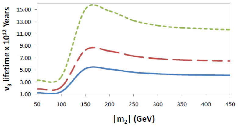
Figure 2: Variation of $\nu_{3}$ lifetime versus $|m_{2}|$ for three values of $\tan\beta$. Starting with the upper curve, $\tan\beta$ = 30, 40, 50. Other parameters have the values $|\mu|=100$, $|f_{3}|=1.5\times 10^{-7}$, $|f_{3}^{\prime}|=2\times 10^{-8}$, $|f_{3}^{\prime\prime}|=8\times 10^{-9}$, $|f_{4}|=|f_{4}^{\prime}|=|f_{4}^{\prime\prime}|=35$, $|f_{5}|=1.01\times 10^{-1}$, $|f_{5}^{\prime}|=5.3\times 10^{-1}$, $|f_{5}^{\prime\prime}|=4\times 10^{-2}$, $m_{N}=200$, $|A_{0}|=500$, $m_{E}=260$, $m_{0}=300$, $\chi_{m_{2}}=1.2$, $\chi_{\mu}=0.8$, $\chi_{3}=0.3$, $\chi_{3}^{\prime}=0.2$, $\chi_{3}^{\prime\prime}=0.6$, $\chi_{4}=1.4$, $\chi_{4}^{\prime}=1.1$, $\chi_{4}^{\prime\prime}=1.7$, $\chi_{5}=1.7$, $\chi_{5}^{\prime}=0.5$, $\chi_{5}^{\prime\prime}=0.7$ and $\chi_{A_{0}}=0.4$. All masses are in GeV and phases in rad.

In Fig. (3) we investigate the effect of the variation of $m_{0}$ on $\nu_{3}$ lifetime, where $m_{0}^{2}=\tilde{M}_{\tau L}^{2}=\tilde{M}_{E}^{2}=\tilde{M}_{\tau}^{2}=\tilde{M}_{\chi}^{2}=\tilde{M}_{\mu L}^{2}=\tilde{M}_{\mu}^{2}=\tilde{M}_{eL}^{2}=\tilde{M}_{e}^{2}$ (see Appendix). Three curves are shown on the figure, corresponding to $\tan\beta$ = 30, 40, 50, starting from the upper curve ($\tan\beta=30$) and going down. The analysis shows that the lifetime of $\nu_{3}$ increases as $m_{0}$ increases. This is as expected since a larger $m_{0}$ implies larger sfermion masses that enter in the loop which gives a smaller decay width and a larger lifetime. It is seen that with values of the input parameters in reasonable ranges the lifetime can be as low as few times $10^{12}$ yrs just within the reach of improved CIB experiment.

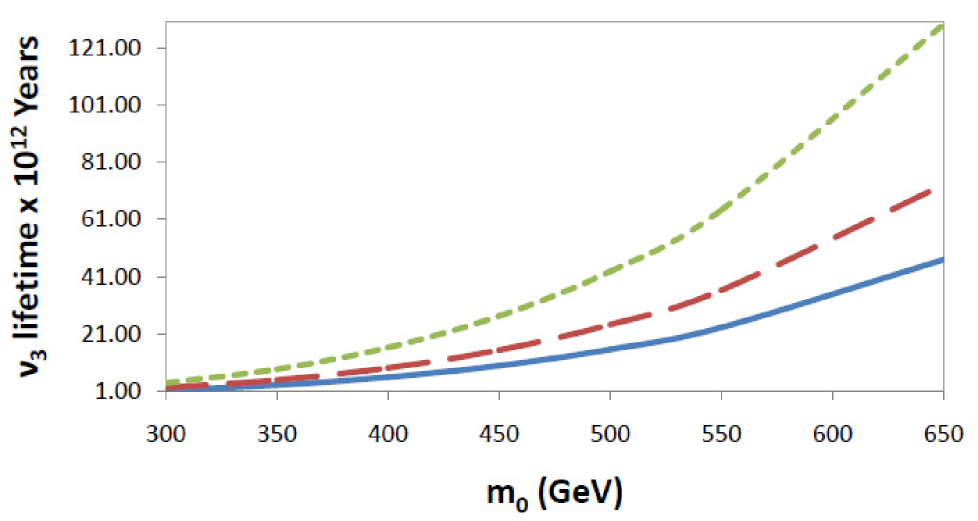
Figure 3: Exhibition of the dependence of $\nu_{3}$ lifetime on $m_{0}$ for three values of $\tan\beta$. Starting with the upper curve, $\tan\beta$ = 30, 40, 50. Other parameters have the values $|\mu|=100$, $|f_{3}|=1.5\times 10^{-7}$, $|f_{3}^{\prime}|=2\times 10^{-8}$, $|f_{3}^{\prime\prime}|=8\times 10^{-9}$, $|f_{4}|=|f_{4}^{\prime}|=|f_{4}^{\prime\prime}|=35$, $|f_{5}|=1.01\times 10^{-1}$, $|f_{5}^{\prime}|=5.3\times 10^{-1}$, $|f_{5}^{\prime\prime}|=4\times 10^{-2}$, $m_{N}=200$, $|A_{0}|=500$, $m_{E}=260$, $|m_{2}|=100$, $\chi_{m_{2}}=1.2$, $\chi_{\mu}=0.8$, $\chi_{3}=0.3$, $\chi_{3}^{\prime}=0.2$, $\chi_{3}^{\prime\prime}=0.6$, $\chi_{4}=1.4$, $\chi_{4}^{\prime}=1.1$, $\chi_{4}^{\prime\prime}=1.7$, $\chi_{5}=1.7$, $\chi_{5}^{\prime}=0.5$, $\chi_{5}^{\prime\prime}=0.7$ and $\chi_{A_{0}}=0.4$. All masses are in GeV and phases in rad.

In Fig. (4) we investigate the effect on $\nu_{3}$ lifetime of the variation of $\chi_{5}$ which is the phase of the coupling term $f_{5}$ in the neutrino mass matrix. The analysis is done for two values of its magnitude $|f_{5}|$ (see the figure caption). The analysis shows that the $\nu_{3}$ lifetime depends sensitively on the phase $\chi_{5}$ and also on its magnitude. Fig. (4) exhibits several oscillations in the lifetime as a function of $\chi_{5}$.

Figure 4: Exhibition of the dependence of $\nu_{3}$ lifetime on the phase $\chi_{5}$ for two values of $|f_{5}|$. Solid curve is for $|f_{5}|$ = 0.1 and dashed curve is for $|f_{5}|$ = 0.05. Other parameters have the values $|m_{2}|=|\mu|=100$, $|f_{3}|=1.5\times 10^{-7}$, $|f_{3}^{\prime}|=2\times 10^{-8}$, $|f_{3}^{\prime\prime}|=8\times 10^{-9}$, $|f_{4}|=|f_{4}^{\prime}|=|f_{4}^{\prime\prime}|=35$, $|f_{5}^{\prime}|=5.3\times 10^{-1}$, $|f_{5}^{\prime\prime}|=4\times 10^{-2}$, $m_{N}=200$, $|A_{0}|=500$, $m_{E}=260$, $m_{0}=300$, $\tan\beta=40$, $\chi_{m_{2}}=1.2$, $\chi_{\mu}=0.8$, $\chi_{3}=0.3$, $\chi_{3}^{\prime}=0.2$, $\chi_{3}^{\prime\prime}=0.6$, $\chi_{4}=1.4$, $\chi_{4}^{\prime}=1.1$, $\chi_{4}^{\prime\prime}=1.7$, $\chi_{5}^{\prime}=1.0$, $\chi_{5}^{\prime\prime}=0.7$ and $\chi_{A_{0}}=0.4$. All masses are in GeV and phases in rad.

One possible origin of such oscillations could be constructive and destructive interference between $F^{jl}_{2~{}left}$ and $F^{jl}_{2~{}right}$, and between $F^{jl}_{3~{}left}$ and $F^{jl}_{3~{}right}$. Such interference was noticed and extensively studied in the context of EDMs of the quarks and the leptons  [23] (for review see  [24, 25]). Some numerical values are exhibited in Table (2). Since $F_{3}$ is much larger than $F_{2}$ for this region of the parameter space, we focus on the $F_{3}$ terms. Here one finds that the $F_{3~{}left}$ is larger than $F_{3~{}right}$ and further each of the terms have phases of the same sign. Thus this possibility does not appear to be the reason for large oscillations in $\nu_{3}$ lifetime. The above suggests that it is the interference in the $F_{3~{}left}$ terms themselves that is the origin of such rapid variation. This can come about because there are sixteen different contribution to $F_{3~{}left}$ each with their own phases and thus multiple constructive and destructive interference can occur which is what Fig. (4) exhibits.

$\chi_{5}$	0.4 rad	1.6 rad
$F^{jl}_{2~{}left}$	$(1.89\times 10^{-20})\exp(+0.34\,i)$	$(3.56\times 10^{-21})\exp(+1.48\,i)$
$F^{jl}_{2~{}right}$	$(5.53\times 10^{-21})\exp(-3.08\,i)$	$(1.39\times 10^{-21})\exp(-1.59\,i)$
$F^{jl}_{2}(0)$	$(1.37\times 10^{-20})\exp(+0.46\,i)$	$(2.17\times 10^{-21})\exp(+1.73\,i)$
$F^{jl}_{3~{}left}$	$(2.49\times 10^{-17})\exp(+0.63\,i)$	$(1.59\times 10^{-18})\exp(-1.60\,i)$
$F^{jl}_{3~{}right}$	$(2.68\times 10^{-18})\exp(+0.67\,i)$	$(1.68\times 10^{-19})\exp(-1.35\,i)$
$F^{jl}_{3}(0)$	$(2.76\times 10^{-17})\exp(+0.64\,i)$	$(1.75\times 10^{-18})\exp(-1.58\,i)$
Decay width	$1.18\times 10^{-44}$ GeV	$7.58\times 10^{-48}$ GeV

Table 2: A list of the right and left contributions, the form factors and the decay width of the process $\nu_{3}\to\nu_{2}+\gamma$ for two values of $\chi_{5}$, with $|f_{5}|$ = 0.1 GeV.

In Fig. (5) we exhibit the variation of the lifetime as a function of the trilinear coupling $|A_{0}|$ for two values of $|\mu|$. In the analysis we make the simple approximation $A_{\tau}=A_{E}=A_{\mu}=A_{e}=A_{0}$.

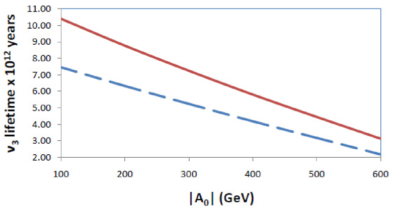
Figure 5: Exhibition of the dependence of $\nu_{3}$ lifetime on $|A_{0}|$ for two values of $|\mu|$. Solid curve is for $|\mu|$ = 150 and dashed curve is for $|\mu|$ = 100. Other parameters have the values $|m_{2}|=100$, $|f_{3}|=1.5\times 10^{-7}$, $|f_{3}^{\prime}|=2\times 10^{-8}$, $|f_{3}^{\prime\prime}|=8\times 10^{-9}$, $|f_{4}|=|f_{4}^{\prime}|=|f_{4}^{\prime\prime}|=35$, $|f_{5}|=1.01\times 10^{-1}$, $|f_{5}^{\prime}|=5.3\times 10^{-1}$, $|f_{5}^{\prime\prime}|=4\times 10^{-2}$, $m_{N}=200$, $m_{E}=260$, $m_{0}=350$, $\tan\beta=50$, $\chi_{m_{2}}=1.2$, $\chi_{\mu}=0.8$, $\chi_{3}=0.3$, $\chi_{3}^{\prime}=0.2$, $\chi_{3}^{\prime\prime}=0.6$, $\chi_{4}=1.4$, $\chi_{4}^{\prime}=1.1$, $\chi_{4}^{\prime\prime}=1.7$, $\chi_{5}=1.7$, $\chi_{5}^{\prime}=0.5$, $\chi_{5}^{\prime\prime}=0.7$ and $\chi_{A_{0}}=0.4$. All masses are in GeV and phases in rad.

Finally we discuss the effect of $|f_{3}|$ on the tau neutrino lifetime. This analysis is exhibited in Fig. (6) for two values of $\tan\beta$ (see figure caption). While $f_{3}$ appears both in the slepton and the neutrino mass matrix, the major effect of $f_{3}$ arises via the variations in the neutrino mass matrix. In summary the analysis of Figs.(2) - (6) shows that the neutrino lifetime as low as the current experimental lower limits can be obtained in models with a vector like generation. These lifetimes are over 30 orders of magnitude smaller than in the Standard Model and thus within the reach of improved experiment.

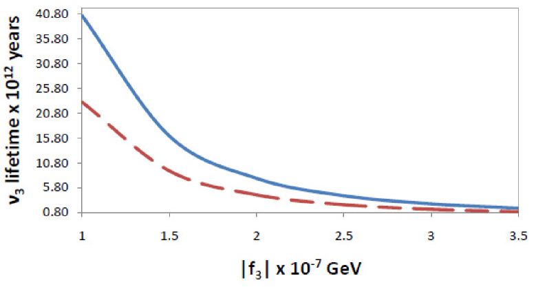
Figure 6: Exhibition of the dependence of the $\nu_{3}$ lifetime on $|f_{3}|$ for two values of $\tan\beta$. Solid curve is for $\tan\beta=30$ and dashed curve is for $\tan\beta=40$. Other parameters have the values $|m_{2}|=100$, $|\mu|=100$, $|f_{3}^{\prime}|=2\times 10^{-8}$, $|f_{3}^{\prime\prime}|=8\times 10^{-9}$, $|f_{4}|=|f_{4}^{\prime}|=|f_{4}^{\prime\prime}|=35$, $|f_{5}|=1.01\times 10^{-1}$, $|f_{5}^{\prime}|=5.3\times 10^{-1}$, $|f_{5}^{\prime\prime}|=4\times 10^{-2}$, $m_{N}=200$, $|A_{0}|=500$, $m_{E}=260$, $m_{0}=400$, $\chi_{m_{2}}=1.2$, $\chi_{\mu}=0.8$, $\chi_{3}=0.3$, $\chi_{3}^{\prime}=0.2$, $\chi_{3}^{\prime\prime}=0.6$, $\chi_{4}=1.4$, $\chi_{4}^{\prime}=1.1$, $\chi_{4}^{\prime\prime}=1.7$, $\chi_{5}=1.7$, $\chi_{5}^{\prime}=0.5$, $\chi_{5}^{\prime\prime}=0.7$ and $\chi_{A_{0}}=0.4$. All masses are in GeV and phases in rad.

6 Conclusion

Lepton flavor changing processes provide an important window to new physics beyond the Standard Model. In this work we have analyzed the radiative decay of the neutrinos $\nu_{i}\to\nu_{j}\gamma$ in an extension of the MSSM with a vector like leptonic multiplet. Specifically we consider mixing between the Standard Model generations of leptons with the mirror leptons in the vector multiplet. It is because of these mixing which are parametrized by $f_{3},f_{4},f_{5}$, $f_{3}^{\prime},f_{4}^{\prime},f_{5}^{\prime}$, $f_{3}^{\prime\prime},f_{4}^{\prime\prime}$ and $f_{5}^{\prime\prime}$ as defined in Eq.(6) that the neutrino can have a radiative decay. The computation of the neutrino decay is done in the supersymmetric sector where we compute the contributions to the neutrino decay arising from diagrams with exchange of charginos and staus in the loop with the chargino or the stau emitting the photon. The effects of CP violation were also included in the analysis. In the presence of CP phases both the magnetic and the electric transition dipole moments contribute to the neutrino lifetime. However, it is found that the electric transition dipole moment often dominates for moderate size CP phases in the region of the parameter space investigated. A numerical analysis shows that the neutrino lifetime can be smaller than the one predicted in the Standard Model by several orders of magnitude. Thus the Standard Model gives a lifetime for the decay of the heaviest neutrino $\nu_{3}$ so that $\tau_{\nu_{3}}^{SM}\sim 10^{43}~{}~{}{\rm yrs}$ for a $\nu_{3}$ with mass 50 meV. However, in the class of models where the three generations of sleptons can mix with the vector like slepton generation one finds that the decay lifetime of $\nu_{3}$ can be as low as $10^{12}$ years and thus much smaller than the Standard Model prediction. Thus improved experiments in the future give the possibility of observation of such effects.

7 Appendix: Further details of the interactions of the vector like multiplet

In this Appendix we give further details of the interactions of the vector like multiplet. The total lagrangian is constituted of ${\cal L}_{F}$ and ${\cal L}_{D}$ where

$${\cal L}_{F}={\cal L}_{L}+{\cal L}_{N}.$$ (32)

Here

$$-{\cal L}_{L}=\left(\frac{v^{2}_{2}|f^{\prime}_{2}|^{2}}{2}+|f_{3}|^{2}+|f_{3}^{\prime}|^{2}+|f_{3}^{\prime\prime}|^{2}\right)\tilde{E}_{R}\tilde{E}^{*}_{R}+\left(\frac{v^{2}_{2}|f^{\prime}_{2}|^{2}}{2}+|f_{4}|^{2}+|f_{4}^{\prime}|^{2}+|f_{4}^{\prime\prime}|^{2}\right)\tilde{E}_{L}\tilde{E}^{*}_{L}$$

$$+\left(\frac{v^{2}_{1}|f_{1}|^{2}}{2}+|f_{4}|^{2}\right)\tilde{\tau}_{R}\tilde{\tau}^{*}_{R}+\left(\frac{v^{2}_{1}|f_{1}|^{2}}{2}+|f_{3}|^{2}\right)\tilde{\tau}_{L}\tilde{\tau}^{*}_{L}$$

$$+\left(\frac{v^{2}_{1}|h_{1}|^{2}}{2}+|f_{4}^{\prime}|^{2}\right)\tilde{\mu}_{R}\tilde{\mu}^{*}_{R}+\left(\frac{v^{2}_{1}|h_{1}|^{2}}{2}+|f_{3}^{\prime}|^{2}\right)\tilde{\mu}_{L}\tilde{\mu}^{*}_{L}$$

$$+\left(\frac{v^{2}_{1}|h_{2}|^{2}}{2}+|f_{4}^{\prime\prime}|^{2}\right)\tilde{e}_{R}\tilde{e}^{*}_{R}+\left(\frac{v^{2}_{1}|h_{2}|^{2}}{2}+|f_{3}^{\prime\prime}|^{2}\right)\tilde{e}_{L}\tilde{e}^{*}_{L}$$

$$+\Bigg{\{}-\frac{f_{1}\mu^{*}v_{2}}{\sqrt{2}}\tilde{\tau}_{L}\tilde{\tau}^{*}_{R}-\frac{h_{1}\mu^{*}v_{2}}{\sqrt{2}}\tilde{\mu}_{L}\tilde{\mu}^{*}_{R}$$

$$-\frac{f^{\prime}_{2}\mu^{*}v_{1}}{\sqrt{2}}\tilde{E}_{L}\tilde{E}^{*}_{R}+\left(\frac{f^{\prime}_{2}v_{2}f^{*}_{3}}{\sqrt{2}}+\frac{f_{4}v_{1}f^{*}_{1}}{\sqrt{2}}\right)\tilde{E}_{L}\tilde{\tau}^{*}_{L}$$

$$+\left(\frac{f_{4}v_{2}f^{\prime*}_{2}}{\sqrt{2}}+\frac{f_{1}v_{1}f^{*}_{3}}{\sqrt{2}}\right)\tilde{E}_{R}\tilde{\tau}^{*}_{R}+\left(\frac{f^{\prime}_{3}v_{2}f^{\prime*}_{2}}{\sqrt{2}}+\frac{h_{1}v_{1}f^{\prime*}_{4}}{\sqrt{2}}\right)\tilde{E}_{L}\tilde{\mu}^{*}_{L}+\left(\frac{f^{\prime}_{2}v_{2}f^{\prime*}_{4}}{\sqrt{2}}+\frac{f^{\prime}_{3}v_{1}h^{*}_{1}}{\sqrt{2}}\right)\tilde{E}_{R}\tilde{\mu}^{*}_{R}$$

$$+\left(\frac{f^{\prime\prime*}_{3}v_{2}f^{\prime}_{2}}{\sqrt{2}}+\frac{f^{\prime\prime}_{4}v_{1}h^{*}_{2}}{\sqrt{2}}\right)\tilde{E}_{L}\tilde{e}^{*}_{L}+\left(\frac{f^{\prime\prime}_{4}v_{2}f^{\prime*}_{2}}{\sqrt{2}}+\frac{f^{\prime\prime*}_{3}v_{1}h^{*}_{2}}{\sqrt{2}}\right)\tilde{E}_{R}\tilde{e}^{*}_{R}$$

$$+f^{\prime}_{3}f^{*}_{3}\tilde{\mu}_{L}\tilde{\tau}^{*}_{L}+f_{4}f^{\prime*}_{4}\tilde{\mu}_{R}\tilde{\tau}^{*}_{R}+f_{4}f^{\prime\prime*}_{4}\tilde{e}_{R}\tilde{\tau}^{*}_{R}+f^{\prime\prime}_{3}f^{*}_{3}\tilde{e}_{L}\tilde{\tau}^{*}_{L}$$

$$+f^{\prime\prime}_{3}f^{\prime*}_{3}\tilde{e}_{L}\tilde{\mu}^{*}_{L}+f^{\prime}_{4}f^{\prime\prime*}_{4}\tilde{e}_{R}\tilde{\mu}^{*}_{R}-\frac{h_{2}\mu^{*}v_{2}}{\sqrt{2}}\tilde{e}_{L}\tilde{e}^{*}_{R}+H.c.\Bigg{\}}$$ (33)

and

$$-{\cal L}_{N}=\left(\frac{v^{2}_{1}|f_{2}|^{2}}{2}+|f_{3}|^{2}+|f_{3}^{\prime}|^{2}+|f_{3}^{\prime\prime}|^{2}\right)\tilde{N}_{R}\tilde{N}^{*}_{R}$$

$$+\left(\frac{v^{2}_{1}|f_{2}|^{2}}{2}+|f_{5}|^{2}+|f_{5}^{\prime}|^{2}+|f_{5}^{\prime\prime}|^{2}\right)\tilde{N}_{L}\tilde{N}^{*}_{L}$$

$$+\left(\frac{v^{2}_{2}|f^{\prime}_{1}|^{2}}{2}+|f_{5}|^{2}\right)\tilde{\nu}_{\tau R}\tilde{\nu}^{*}_{\tau R}+\left(\frac{v^{2}_{2}|f^{\prime}_{1}|^{2}}{2}+|f_{3}|^{2}\right)\tilde{\nu}_{\tau L}\tilde{\nu}^{*}_{\tau L}$$

$$+\left(\frac{v^{2}_{2}|h^{\prime}_{1}|^{2}}{2}+|f_{3}^{\prime}|^{2}\right)\tilde{\nu}_{\mu L}\tilde{\nu}^{*}_{\mu L}+\left(\frac{v^{2}_{2}|h^{\prime}_{1}|^{2}}{2}+|f_{5}^{\prime}|^{2}\right)\tilde{\nu}_{\mu R}\tilde{\nu}^{*}_{\mu R}$$

$$+\left(\frac{v^{2}_{2}|h^{\prime}_{2}|^{2}}{2}+|f_{3}^{\prime\prime}|^{2}\right)\tilde{\nu}_{eL}\tilde{\nu}^{*}_{eL}+\left(\frac{v^{2}_{2}|h^{\prime}_{2}|^{2}}{2}+|f_{5}^{\prime\prime}|^{2}\right)\tilde{\nu}_{eR}\tilde{\nu}^{*}_{eR}$$

$$+\Bigg{\{}-\frac{f_{2}\mu^{*}v_{2}}{\sqrt{2}}\tilde{N}_{L}\tilde{N}^{*}_{R}-\frac{f^{\prime}_{1}\mu^{*}v_{1}}{\sqrt{2}}\tilde{\nu}_{\tau L}\tilde{\nu}^{*}_{\tau R}-\frac{h^{\prime}_{1}\mu^{*}v_{1}}{\sqrt{2}}\tilde{\nu}_{\mu L}\tilde{\nu}^{*}_{\mu R}$$

$$+\left(\frac{f_{5}v_{2}f^{\prime*}_{1}}{\sqrt{2}}-\frac{f_{2}v_{1}f^{*}_{3}}{\sqrt{2}}\right)\tilde{N}_{L}\tilde{\nu}^{*}_{\tau L}+\left(\frac{f_{5}v_{1}f^{*}_{2}}{\sqrt{2}}-\frac{f^{\prime}_{1}v_{2}f^{*}_{3}}{\sqrt{2}}\right)\tilde{N}_{R}\tilde{\nu}^{*}_{\tau R}$$

$$+\left(\frac{h^{\prime}_{1}v_{2}f^{\prime*}_{5}}{\sqrt{2}}-\frac{f^{\prime}_{3}v_{1}f^{*}_{2}}{\sqrt{2}}\right)\tilde{N}_{L}\tilde{\nu}^{*}_{\mu L}+\left(\frac{f^{\prime\prime}_{5}v_{1}f^{*}_{2}}{\sqrt{2}}-\frac{f^{\prime\prime*}_{3}v_{2}h^{\prime}_{2}}{\sqrt{2}}\right)\tilde{N}_{R}\tilde{\nu}^{*}_{eR}$$

$$+\left(\frac{h^{\prime*}_{2}v_{2}f^{\prime\prime}_{5}}{\sqrt{2}}-\frac{f^{\prime\prime*}_{3}v_{1}f_{2}}{\sqrt{2}}\right)\tilde{N}_{L}\tilde{\nu}^{*}_{eL}+\left(\frac{f^{\prime}_{5}v_{1}f^{*}_{2}}{\sqrt{2}}-\frac{h^{\prime}_{1}v_{2}f^{\prime*}_{3}}{\sqrt{2}}\right)\tilde{N}_{R}\tilde{\nu}^{*}_{\mu R}$$

$$+f^{\prime}_{3}f^{*}_{3}\tilde{\nu}_{\mu L}\tilde{\nu}_{\tau^{*}_{L}}+f_{5}f^{\prime*}_{5}\tilde{\nu}_{\mu R}\tilde{\nu}^{*}_{\tau R}-\frac{h^{\prime}_{2}\mu^{*}v_{1}}{\sqrt{2}}\tilde{\nu}_{eL}\tilde{\nu}^{*}_{eR}$$

$$+f^{\prime\prime}_{3}f^{*}_{3}\tilde{\nu}_{eL}\tilde{\nu}^{*}_{\tau L}+f_{5}f^{\prime\prime*}_{5}\tilde{\nu}_{eR}\tilde{\nu}^{*}_{\tau R}+f^{\prime\prime}_{3}f^{\prime*}_{3}\tilde{\nu}_{eL}\tilde{\nu}^{*}_{\mu L}+f^{\prime}_{5}f^{\prime\prime*}_{5}\tilde{\nu}_{eR}\tilde{\nu}^{*}_{\mu R}+H.c.\Bigg{\}}.$$ (34)

Similarly the mass terms arising from the D term are given by

$$-{\cal L}_{D}=\frac{1}{2}m^{2}_{Z}\cos^{2}\theta_{W}\cos 2\beta\{\tilde{\nu}_{\tau L}\tilde{\nu}^{*}_{\tau L}-\tilde{\tau}_{L}\tilde{\tau}^{*}_{L}+\tilde{\nu}_{\mu L}\tilde{\nu}^{*}_{\mu L}-\tilde{\mu}_{L}\tilde{\mu}^{*}_{L}$$

$$+\tilde{\nu}_{eL}\tilde{\nu}^{*}_{eL}-\tilde{e}_{L}\tilde{e}^{*}_{L}+\tilde{E}_{R}\tilde{E}^{*}_{R}-\tilde{N}_{R}\tilde{N}^{*}_{R}\}$$

$$+\frac{1}{2}m^{2}_{Z}\sin^{2}\theta_{W}\cos 2\beta\{\tilde{\nu}_{\tau L}\tilde{\nu}^{*}_{\tau L}$$

$$+\tilde{\tau}_{L}\tilde{\tau}^{*}_{L}+\tilde{\nu}_{\mu L}\tilde{\nu}^{*}_{\mu L}+\tilde{\mu}_{L}\tilde{\mu}^{*}_{L}+\tilde{\nu}_{eL}\tilde{\nu}^{*}_{eL}+\tilde{e}_{L}\tilde{e}^{*}_{L}$$

$$-\tilde{E}_{R}\tilde{E}^{*}_{R}-\tilde{N}_{R}\tilde{N}^{*}_{R}+2\tilde{E}_{L}\tilde{E}^{*}_{L}-2\tilde{\tau}_{R}\tilde{\tau}^{*}_{R}-2\tilde{\mu}_{R}\tilde{\mu}^{*}_{R}-2\tilde{e}_{R}\tilde{e}^{*}_{R}\}.$$ (35)

In addition we have the following set of soft breaking terms

$$V_{soft}=\tilde{M}^{2}_{\tau L}\tilde{\psi}^{i*}_{\tau L}\tilde{\psi}^{i}_{\tau L}+\tilde{M}^{2}_{\chi}\tilde{\chi}^{ci*}\tilde{\chi}^{ci}$$

$$+\tilde{M}^{2}_{\mu L}\tilde{\psi}^{i*}_{\mu L}\tilde{\psi}^{i}_{\mu L}+\tilde{M}^{2}_{eL}\tilde{\psi}^{i*}_{eL}\tilde{\psi}^{i}_{eL}+\tilde{M}^{2}_{\nu_{\tau}}\tilde{\nu}^{c*}_{\tau L}\tilde{\nu}^{c}_{\tau L}$$

$$+\tilde{M}^{2}_{\nu_{\mu}}\tilde{\nu}^{c*}_{\mu L}\tilde{\nu}^{c}_{\mu L}+\tilde{M}^{2}_{\nu_{e}}\tilde{\nu}^{c*}_{eL}\tilde{\nu}^{c}_{eL}+\tilde{M}^{2}_{\tau}\tilde{\tau}^{c*}_{L}\tilde{\tau}^{c}_{L}$$

$$+\tilde{M}^{2}_{\mu}\tilde{\mu}^{c*}_{L}\tilde{\mu}^{c}_{L}+\tilde{M}^{2}_{e}\tilde{e}^{c*}_{L}\tilde{e}^{c}_{L}+\tilde{M}^{2}_{E}\tilde{E}^{*}_{L}\tilde{E}_{L}+\tilde{M}^{2}_{N}\tilde{N}^{*}_{L}\tilde{N}_{L}$$

$$+\epsilon_{ij}\{f_{1}A_{\tau}H^{i}_{1}\tilde{\psi}^{j}_{\tau L}\tilde{\tau}^{c}_{L}-f^{\prime}_{1}A_{\nu_{\tau}}H^{i}_{2}\tilde{\psi}^{j}_{\tau L}\tilde{\nu}^{c}_{\tau L}$$

$$+h_{1}A_{\mu}H^{i}_{1}\tilde{\psi}^{j}_{\mu L}\tilde{\mu}^{c}_{L}-h^{\prime}_{1}A_{\nu_{\mu}}H^{i}_{2}\tilde{\psi}^{j}_{\mu L}\tilde{\nu}^{c}_{\mu L}$$

$$+h_{2}A_{e}H^{i}_{1}\tilde{\psi}^{j}_{eL}\tilde{e}^{c}_{L}-h^{\prime}_{2}A_{\nu_{e}}H^{i}_{2}\tilde{\psi}^{j}_{eL}\tilde{\nu}^{c}_{eL}$$

$$+f_{2}A_{N}H^{i}_{1}\tilde{\chi}^{cj}\tilde{N}_{L}-f^{\prime}_{2}A_{E}H^{i}_{2}\tilde{\chi}^{cj}\tilde{E}_{L}+H.c.\}$$ (36)

From ${\cal L}_{F,D}$ and by giving the neutral Higgs their vacuum expectation values in $V_{soft}$ we can produce the mass squared matrix $M^{2}_{\tilde{\tau}}$ in the basis $(\tilde{\tau}_{L},\tilde{E}_{L},\tilde{\tau}_{R},\tilde{E}_{R},\tilde{\mu}_{L},\tilde{\mu}_{R},\tilde{e}_{L},\tilde{e}_{R})$. We label the matrix elements of these as $(M^{2}_{\tilde{\tau}})_{ij}=M^{2}_{ij}$ where

$$M^{2}_{11}=\tilde{M}^{2}_{\tau L}+\frac{v^{2}_{1}|f_{1}|^{2}}{2}+|f_{3}|^{2}-m^{2}_{Z}\cos 2\beta\left(\frac{1}{2}-\sin^{2}\theta_{W}\right),$$

$$M^{2}_{22}=\tilde{M}^{2}_{E}+\frac{v^{2}_{2}|f^{\prime}_{2}|^{2}}{2}+|f_{4}|^{2}+|f^{\prime}_{4}|^{2}+|f^{\prime\prime}_{4}|^{2}+m^{2}_{Z}\cos 2\beta\sin^{2}\theta_{W},$$

$$M^{2}_{33}=\tilde{M}^{2}_{\tau}+\frac{v^{2}_{1}|f_{1}|^{2}}{2}+|f_{4}|^{2}-m^{2}_{Z}\cos 2\beta\sin^{2}\theta_{W},$$

$$M^{2}_{44}=\tilde{M}^{2}_{\chi}+\frac{v^{2}_{2}|f^{\prime}_{2}|^{2}}{2}+|f_{3}|^{2}+|f^{\prime}_{3}|^{2}+|f^{\prime\prime}_{3}|^{2}+m^{2}_{Z}\cos 2\beta\left(\frac{1}{2}-\sin^{2}\theta_{W}\right),$$

$$M^{2}_{55}=\tilde{M}^{2}_{\mu L}+\frac{v^{2}_{1}|h_{1}|^{2}}{2}+|f^{\prime}_{3}|^{2}-m^{2}_{Z}\cos 2\beta\left(\frac{1}{2}-\sin^{2}\theta_{W}\right),$$

$$M^{2}_{66}=\tilde{M}^{2}_{\mu}+\frac{v^{2}_{1}|h_{1}|^{2}}{2}+|f^{\prime}_{4}|^{2}-m^{2}_{Z}\cos 2\beta\sin^{2}\theta_{W},$$

$$M^{2}_{77}=\tilde{M}^{2}_{eL}+\frac{v^{2}_{1}|h_{2}|^{2}}{2}+|f^{\prime\prime}_{3}|^{2}-m^{2}_{Z}\cos 2\beta\left(\frac{1}{2}-\sin^{2}\theta_{W}\right),$$

$$M^{2}_{88}=\tilde{M}^{2}_{e}+\frac{v^{2}_{1}|h_{2}|^{2}}{2}+|f^{\prime\prime}_{4}|^{2}-m^{2}_{Z}\cos 2\beta\sin^{2}\theta_{W},$$

$$M^{2}_{12}=M^{2*}_{21}=\frac{v_{2}f^{\prime}_{2}f^{*}_{3}}{\sqrt{2}}+\frac{v_{1}f_{4}f^{*}_{1}}{\sqrt{2}},$$

$$M^{2}_{13}=M^{2*}_{31}=\frac{f^{*}_{1}}{\sqrt{2}}(v_{1}A^{*}_{\tau}-\mu v_{2}),$$

$$M^{2}_{14}=M^{2*}_{41}=0,M^{2}_{15}=M^{2*}_{51}=f^{\prime}_{3}f^{*}_{3},$$

$$M^{2*}_{16}=M^{2*}_{61}=0,M^{2*}_{17}=M^{2*}_{71}=f^{\prime\prime}_{3}f^{*}_{3},M^{2*}_{18}=M^{2*}_{81}=0,M^{2}_{23}=M^{2*}_{32}=0,$$

$$M^{2}_{24}=M^{2*}_{42}=\frac{f^{\prime*}_{2}}{\sqrt{2}}(v_{2}A^{*}_{E}-\mu v_{1}),M^{2}_{25}=M^{2*}_{52}=\frac{v_{2}f^{\prime}_{3}f^{\prime*}_{2}}{\sqrt{2}}+\frac{v_{1}h_{1}f^{*}_{4}}{\sqrt{2}},$$

$$M^{2}_{26}=M^{2*}_{62}=0,M^{2}_{27}=M^{2*}_{72}=\frac{v_{2}f^{\prime\prime}_{3}f^{\prime*}_{2}}{\sqrt{2}}+\frac{v_{1}h_{1}f^{\prime*}_{4}}{\sqrt{2}},M^{2}_{28}=M^{2*}_{82}=0,$$

$$M^{2}_{34}=M^{2*}_{43}=\frac{v_{2}f_{4}f^{\prime*}_{2}}{\sqrt{2}}+\frac{v_{1}f_{1}f^{*}_{3}}{\sqrt{2}},M^{2}_{35}=M^{2*}_{53}=0,M^{2}_{36}=M^{2*}_{63}=f_{4}f^{\prime*}_{4},$$

$$M^{2}_{37}=M^{2*}_{73}=0,M^{2}_{38}=M^{2*}_{83}=f_{4}f^{\prime\prime*}_{4},M^{2}_{45}=M^{2*}_{54}=0,M^{2}_{46}=M^{2*}_{64}=\frac{v_{2}f^{\prime}_{2}f^{\prime*}_{4}}{\sqrt{2}}+\frac{v_{1}f^{\prime}_{3}h^{*}_{1}}{\sqrt{2}},$$

$$M^{2}_{47}=M^{2*}_{74}=0,M^{2}_{48}=M^{2*}_{84}=\frac{v_{2}f^{\prime}_{2}f^{\prime\prime*}_{4}}{\sqrt{2}}+\frac{v_{1}f^{\prime\prime}_{3}h^{*}_{2}}{\sqrt{2}},$$

$$M^{2}_{56}=M^{2*}_{65}=\frac{h^{*}_{1}}{\sqrt{2}}(v_{1}A^{*}_{\mu}-\mu v_{2}),M^{2}_{57}=M^{2*}_{75}=f^{\prime\prime}_{3}f^{\prime*}_{3},M^{2}_{58}=M^{2*}_{85}=0,M^{2}_{67}=M^{2*}_{76}=0,$$

$$M^{2}_{68}=M^{2*}_{86}=f^{\prime}_{4}f^{\prime\prime*}_{4},M^{2}_{78}=M^{2*}_{87}=\frac{h^{*}_{2}}{\sqrt{2}}(v_{1}A^{*}_{e}-\mu v_{2})$$ (37)

Here the terms $M^{2}_{11},M^{2}_{13},M^{2}_{31},M^{2}_{33}$ arise from soft breaking in the sector $\tilde{\tau}_{L},\tilde{\tau}_{R}$, the terms $M^{2}_{55},M^{2}_{56},M^{2}_{65},M^{2}_{66}$ arise from soft breaking in the sector $\tilde{\mu}_{L},\tilde{\mu}_{R}$, the terms $M^{2}_{77},M^{2}_{78},M^{2}_{87},M^{2}_{88}$ arise from soft breaking in the sector $\tilde{e}_{L},\tilde{e}_{R}$ and the terms $M^{2}_{22},M^{2}_{24},$ $M^{2}_{42},M^{2}_{44}$ arise from soft breaking in the sector $\tilde{E}_{L},\tilde{E}_{R}$. The other terms arise from mixing between the staus, smuons and the mirrors. We assume that all the masses are of the electroweak size so all the terms enter in the mass squared matrix. We diagonalize this hermitian mass squared matrix by the unitary transformation $\tilde{D}^{\tau\dagger}M^{2}_{\tilde{\tau}}\tilde{D}^{\tau}=diag(M^{2}_{\tilde{\tau}_{1}},M^{2}_{\tilde{\tau}_{2}},M^{2}_{\tilde{\tau}_{3}},M^{2}_{\tilde{\tau}_{4}},M^{2}_{\tilde{\tau}_{5}},M^{2}_{\tilde{\tau}_{6}},M^{2}_{\tilde{\tau}_{7}},M^{2}_{\tilde{\tau}_{8}})$. For a further clarification of the notation see [12]).

Acknowledgments: One of the authors (PN) acknowledges the hospitality of KITP, Santa Barbara, where part of this work was done. This research was supported in part by the National Science Foundation under Grant Nos. PHY-0757959, PHY-0704067 and NSF PHY11-25915.

References

- [1] P. B. Pal and L. Wolfenstein, Phys. Rev. D 25, 766 (1982); K. Sato and M. Kobayashi, Prog. Theor. Phys. 58, 1775 (1977); R. E. Shrock, Nucl. Phys. B 206, 359 (1982); M. A. B. Beg, W. J. Marciano and M. Ruderman, Phys. Rev. D 17, 1395 (1978).
- [2] S. Matsuura, M. Shirahata, M. Kawada, T. T. Takeuchi, D. Burgarella, D. L. Clements, W. -S. Jeong and H. Hanami et al., Astrophys. J. 737, 2 (2011) [arXiv:1002.3674 [astro-ph.CO]].
- [3] H. Dole, G. Lagache, J. -L. Puget, K. I. Caputi, N. Fernandez-Conde, E. Le Floc’h, C. Papovich and P. G. Perez-Gonzalez et al., Astron. Astrophys. 451, 417 (2006) [astro-ph/0603208].
- [4] S. Berta, B. Magnelli, D. Lutz, B. Altieri, H. Aussel, P. Andreani, O. Bauer and A. Bongiovanni et al., arXiv:1005.1073 [astro-ph.CO].
- [5] A. Mirizzi, D. Montanino and P. D. Serpico, Phys. Rev. D 76, 053007 (2007) [arXiv:0705.4667 [hep-ph]].
- [6] S. -H. Kim, K. -i. Takemasa, Y. Takeuchi and S. Matsuura, J. Phys. Soc. Jap. 81, 024101 (2012) [arXiv:1112.4568 [hep-ph]].
- [7] J. Maalampi, J. T. Peltoniemi and M. Roos, Phys. Lett. B 220, 441 (1989).
- [8] T. Ibrahim and P. Nath, Phys. Rev. D 78, 075013 (2008) [arXiv:0806.3880 [hep-ph]].
- [9] T. Ibrahim and P. Nath, Phys. Rev. D 81, 033007 (2010) [arXiv:1001.0231 [hep-ph]].
- [10] T. Ibrahim and P. Nath, Phys. Rev. D 84, 015003 (2011) [arXiv:1104.3851 [hep-ph]].
- [11] T. Ibrahim and P. Nath, Phys. Rev. D 82, 055001 (2010) [arXiv:1007.0432 [hep-ph]].
- [12] T. Ibrahim and P. Nath, Phys. Rev. D 87, 015030 (2013) [arXiv:1211.0622 [hep-ph]].
- [13] T. Ibrahim and P. Nath, Nucl. Phys. Proc. Suppl. 200-202, 161 (2010) [arXiv:0910.1303 [hep-ph]].
- [14] K. S. Babu, I. Gogoladze, M. U. Rehman and Q. Shafi, Phys. Rev. D 78, 055017 (2008).
- [15] C. Liu, Phys. Rev. D 80, 035004 (2009) [arXiv:0907.3011 [hep-ph]].
- [16] S. P. Martin, Phys. Rev. D 81, 035004 (2010) [arXiv:0910.2732 [hep-ph]]; Phys. Rev. D 82, 055019 (2010) [arXiv:1006.4186 [hep-ph]]; Phys. Rev. D 83, 035019 (2011) [arXiv:1012.2072 [hep-ph]].
- [17] P. W. Graham, A. Ismail, S. Rajendran and P. Saraswat, arXiv:0910.3020 [hep-ph].
- [18] J. L. Hewett, H. Weerts, R. Brock, J. N. Butler, B. C. K. Casey, J. Collar, A. de Govea and R. Essig et al., arXiv:1205.2671 [hep-ex].
- [19] P. A. R. Ade et al. [Planck Collaboration], arXiv:1303.5062 [astro-ph.CO].
- [20] T. Schwetz, M. A. Tortola and J. W. F. Valle, New J. Phys. 10, 113011 (2008) [arXiv:0808.2016 [hep-ph]]. See also M. C. Gonzalez-Garcia, M. Maltoni, J. Salvado and T. Schwetz, JHEP 1212, 123 (2012) [arXiv:1209.3023 [hep-ph]].
- [21] F. Gabbiani, A. Masiero and D. W. Sciama, Phys. Lett. B 259, 323 (1991).
- [22] H. Georgi, Nucl. Phys. B 156, 126 (1979); F. Wilczek and A. Zee, Phys. Rev. D 25, 553 (1982); J. Maalampi, J.T. Peltoniemi, and M. Roos, PLB 220, 441(1989); J. Maalampi and M. Roos, Phys. Rept. 186, 53 (1990); K. S. Babu, I. Gogoladze, P. Nath and R. M. Syed, Phys. Rev. D 72, 095011 (2005) [hep-ph/0506312]; Phys. Rev. D 74, 075004 (2006), [arXiv:hep-ph/0607244]; Phys. Rev. D 85, 075002 (2012) [arXiv:1112.5387 [hep-ph]]; P. Nath and R. M. Syed, Phys. Rev. D 81, 037701 (2010).
- [23] T. Ibrahim and P. Nath, Phys. Lett. B 418 (1998) 98 [hep-ph/9707409]; Phys. Rev. D 57 (1998) 478 [hep-ph/9708456]; Phys. Rev. D 61 (2000) 093004 [hep-ph/9910553]; M. Brhlik, G. J. Good and G. L. Kane, Phys. Rev. D 59, 115004 (1999) [hep-ph/9810457].
- [24] T. Ibrahim and P. Nath, Rev. Mod. Phys. 80, 577 (2008); arXiv:hep-ph/0210251. A. Pilaftsis, hep-ph/9908373.
- [25] P. Nath, B. D. Nelson, H. Davoudiasl, B. Dutta, D. Feldman, Z. Liu, T. Han and P. Langacker et al., Nucl. Phys. Proc. Suppl. 200-202, 185 (2010) [arXiv:1001.2693 [hep-ph]].