Magnetospheric “anti-glitches” in magnetars

Abstract

We attribute the rapid spindown of magnetar 1E 2259+586 observed by Archibald et al.  (2013), termed the “anti-glitch”, to partial opening of the magnetosphere during the $X$-ray burst, followed by changes of the structure of the closed field line region. To account for the observed spin decrease during the $X$-ray flare all that is needed is the transient opening, for just one period, of a relatively small fraction of the magnetosphere, of the order of only few percent. More generally, we argue that in magnetars all timing irregularities have magnetospheric origin and are induced either by (i) the fluctuations in the current structure of the magnetosphere (similar to the long term torque variations in the rotationally powered pulsars); or, specifically to magnetars, by (ii) opening of a fraction of the magnetosphere during bursts and flares - the latter events are always accompanied by rapid spindown, an “anti-glitch”. Slow rotational motion of the neutron star crust, driven by crustal magnetic fields, leads beyond some twist limit to explosive instability of the external magnetic fields and transient opening of a large magnetic flux in a CME-type event, the post-flares increase of magnetospheric currents accompanied by enhanced $X$-luminosity and spindown rate, changing profiles, as well as spectral hardening, all in agreement with the magnetospheric model of torque fluctuations.

1 Magnetars’ bursts and flares

Magnetar emission (Woods & Thompson, 2006) is powered by dissipation of a non-potential (current-carrying) magnetic field (Thompson et al., 2002). The magnetic field exerts Lorentz force on the crust, which is balanced by induced elastic stress. For strong enough magnetic fields, Lorentz force may induce a stress that exceeds the critical stress of the lattice, leading to crustal failure. This leads to lattice failure of the crust (Horowitz et al., 2011), which can be either in a form of fast propagating crack (Thompson & Duncan, 1995) (and sudden untwisting of the internal magnetic field) or a slowly (plastically) propagating fault (Jones, 2003) that leads to slow evolution of the external magnetic fields  (Lyutikov, 2006). In the latter case twisting of the external magnetic fields  leads to a sudden relaxation of the twist outside of the star in analogy with solar flares and Coronal Mass Ejections (CMEs) (Forbes et al., 2006; Lyutikov, 2006; Parfrey et al., 2012). Perhaps the best argument in favor of magnetic storage of energy outside of the star is a very short rise time of the 2004 giant flares, $\sim 0.25$ msec (Palmer et al., 2005). This points to the magnetospheric origin of giant flares (Lyutikov, 2006).

Thompson et al. (2002) developed a model of the emission and spin-down behavior of the Anomalous X-ray Pulsars (AXPs) and Soft Gamma-ray Repeaters (SGRs) in which the dissipation of magnetic fields powers its unusually bright X-ray luminosity. In this model the magnetic fields anchored in a well conducting stellar interior are dissipated in the magnetosphere. Wolfson (1995); Thompson et al. (2002); Pavan et al. (2009) constructed a self-similar force-free current-carrying magnetosphere in which the current twist the field lines and causes them to expand with respect to a potential dipole field. Expansion of field lines results in a changing torque on the neutron star which is observed as a variable spin-down rate. Since the X-ray luminosity is proportional to the strength of the currents flowing in the magnetosphere, one expects that spin-down rate is positively correlated with luminosity.

Lyutikov (2006) (see also Parfrey et al. (2012)) proposed that magnetar flares are magnetospheric (and not crustal) events similar to the Solar flares and CMEs. According to Lyutikov (2006) magnetars bursts and flares are driven by unwinding of the internal non-potential magnetic field which leads to a slow build-up of magnetic energy outside of the neutron star. For large magnetospheric currents, corresponding to a large twist of the external magnetic field, magnetosphere becomes dynamically unstable on the Alfvén crossing times scale of the inner magnetosphere. The reconnection processes, e.g., the tearing mode, in the strongly magnetized plasma of magnetar magnetospheres  develops similarly to the non- relativistic plasmas (Lyutikov, 2003; Komissarov et al., 2007).

In addition, current carrying charges resonantly scatter thermal photons from the surface producing through multiple resonant scattering (resonant Comptonization) a non-thermal power-law X-ray tail (Lyutikov & Gavriil, 2006; Fernández & Thompson, 2007; Rea et al., 2008; Beloborodov, 2013). The hardness of the power-law depends on the typical velocity of the current carrying particles and their density. For larger densities (and larger currents) a given photon has a larger probability to be scattered at the cyclotron resonance and thus will experience greater amount of scattering, gaining energy stochastically in each scattering through Doppler effect. Thus, there is a natural prediction of the model by Lyutikov & Gavriil (2006), that the harness of the power-law X-ray tail should correlate positively with the spin down rate and the $X$-ray luminosity.

As we discuss below, the observations of the rapid spindown of the magnetar 1E 2259+586 (Archibald et al., 2013) are in general agreement with the magnetospheric model. Thus, they are qualitatively different form glitches in the rotationally powered pulsar, where they are driven by the presence of a faster component inside the neutron star.

2 Observations of the “anti-glitch” in magnetar 1E 2259+586

Archibald et al. (2013) reported a fast change of the rotation frequency of the magnetar 1E 2259+586, which occurred within two weeks of a bright $X$-ray flare. The accumulated change in frequency was $\Delta\nu\sim 10^{-7}$ Hz over two weeks. For approximately a few months after the flare both the flux and the spindown rate were about two times larger than normal. In addition, the flux increase was also accompanied by hardening of the spectrum and a change in the pulse profile. Importantly, there was a GBM burst, presumably associated with the glitch, with peak luminosity of the order $10^{38}$ erg s^-1 and duration of $\sim 100$ milliseconds.

By analogy with glitches in radio pulsar, except, importantly, for the different sing of the period change, the preferred interpretation of Archibald et al. (2013) for the rapid spindown is a glitch internal to the neutron star. This requires a neutron star component that rotates slower than the crust. The origin of such a component is not obvious (see, though, Thompson et al., 2000).

In radio pulsars the notion of a glitch is usually referred to a sudden change of the spin frequency, on time scale comparable to the pulsar period. In magnetars, the timing measurements are usually separated by about a week. In case of 1E 2259+586, the anti-glitch could be a sudden event, on the time scale of rotation, as well due to enhanced spindown rate by an order of magnitude over approximately a week.

Below we discuss an interpretation alternative to that of Archibald et al. (2013). We argue that all the spin-down activity, as well as spectrum hardening, flux increase and profile changes during the activity period, can be explained via purely magnetospheric effects within the twisted magnetosphere model of Thompson et al. (2002) described above, plus an additional effect of opening the magnetosphere during the prompt burst (Lyutikov, 2006). Thus, we envision that a large spindown occurred during an opening of a modest fraction of the magnetosphere, on a time scale as short as one rotation, followed by an extended period of high spin-down rate, driven by the magnetospheric currents.

3 Twisted Force-Free Equilibria

In this Section we review the solution of Wolfson (1995); Thompson et al. (2002) (see also Gourgouliatos (2008); Pavan et al. (2009)), giving a few simple approximations that are later used for numerical estimates. In a static force-free approximation the electric current flows along magnetic field,

$${\bf\nabla}\times{\bf B}=\alpha({\cal P}){\bf B}.$$ (1)

The non-rotating magnetic equilibria are then described by the second-order elliptic differential equation, the Grad-Shafranov equation (Shafranov, 1966):

$${\bf\nabla}\left({1\over r^{2}\sin^{2}\theta}{\bf\nabla}{\cal P}\right)+{1\over r^{2}\sin^{2}\theta}I{dI\over d{\cal P}}=0$$ (2)

where poloidal and toroidal fields are

$${\bf B}_{P}={{\bf\nabla}{\cal P}\times{\hat{\phi}}\over r\sin\theta},\,{\bf B}_{T}=-{2I\over r\sin\theta}{\hat{\phi}}$$ (3)

$I=I({\cal P})$ is the total current enclosed by the magnetic flux surfaces ${\cal P}$. Choosing separable solutions, and assuming that the current function is a power-law, $I\sim{\cal P}^{(1+p)/p}$, Eq. (2) becomes

$$r^{2}{{\cal R}^{\prime\prime}_{rr}\over{\cal R}}+(1-\mu^{2}){F^{\prime\prime}_{\mu\mu}\over F}+C{r^{2}\over r_{\ast}^{2}}\left({\cal R}F\right)^{2/p}=0$$ (4)

where $C$ is some dimensionless constant related to the strength of the currents ($I\propto\sqrt{Cp/(p+1)}{\cal P}^{(1+p)/p}$) and $r_{\ast}$ is a radius of a neutron star. Separable solutions of Eq. (4) satisfy

$${\cal R}\sim\tilde{r}^{-p}\mbox{}$$

$$p(p+1)F+(1-\mu^{2}){\partial^{2}F\over\partial\mu^{2}}=-CF^{(p+2)/p}$$ (5)

where $\tilde{r}=r/r_{\ast}$ has been introduced.

The current-free case comprises the monopole solution $p=0$ (with an equatorial current sheet), and vacuum multipolar solutions $p=1,2,....$. For non-integer $p$ system (5) gives current-carrying solutions of type considered by Lynden-Bell & Boily (1994). Magnetic fields and current densities are then given by

$${B_{r}\over B_{\ast}}=-{F^{\prime}(\mu)\over 2\tilde{r}^{p+2}}\mbox{}$$

$${B_{\theta}\over B_{\ast}}={pF\over 2\sqrt{1-\mu^{2}}\tilde{r}^{p+2}}\mbox{}$$

$${B_{\phi}\over B_{\theta}}=-\left[{C\over p(1+p)}\right]^{1/2}\,F^{1/p}\mbox{}$$

$$j_{\phi}{cr_{\ast}\over 4\pi B_{\ast}}=-{CF^{(p+2)/p}\over\sqrt{1-\mu^{2}}r^{(3+p)}}\mbox{}$$

$$j_{\theta}{cr_{\ast}\over 4\pi B_{\ast}}=-\sqrt{{pC\over p+1}}{pF^{(p+1)/p}\over r^{(p+2)}\sqrt{1-\mu^{2}}}\mbox{}$$

$${j_{r}}{cr_{\ast}\over 4\pi B_{\ast}}=-\sqrt{{C(1+p)\over p}}{1\over\tilde{r}^{(p+2)}}F^{1/p}F^{\prime}$$ (6)

Comparing with equation (1) shows that $\alpha({\cal P})$ is proportional to ${\cal P}^{1/p}$, and on dimensional grounds one can write

$$\alpha({\cal P})={C^{1/2}\over r_{\rm\ast}}\left({p+1\over p}\right)^{1/2}\,\left({{\cal P}\over{\cal P}_{0}}\right)^{1/p}$$ (7)

The poloidal components of Eq. (1) can be integrated to give

$$B_{\phi}={\int\alpha({\cal P})\,d{\cal P}\over r\sin\theta}={p\over p+1}\,{{\cal P}\alpha({\cal P})\over r\sin\theta}.$$ (8)

Substituting Eqs. (3)-(8) into the $\phi$-component of Eq. (1) then gives the non-linear equation (5) for the angular function $F=F(\mu)$.

The solution of Eq. (5), including the dependence $p(C)$, is uniquely defined by the parameter $C$ and by the three boundary conditions. The first is the requirement of zero $B_{\phi}$ at the polar axis (absence of line current): $B_{\phi}(\mu=1)\propto F(1)=0$ (nonzero $B_{\phi}$ at the polar axis implies a line current), another is overall normalization of the field which we take to be $F^{\prime}={\rm const}=-2$ at $\mu=1$ (corresponding to a fixed flux density $B_{\rm\ast}$ at the magnetic pole). The third boundary condition specifies the multipole structure of the magnetic field at small currents. For dipole field $B_{R}\propto F^{\prime}=0$ at $\mu=0$, for quadrupole field $B_{\theta}\propto F=0$ at $\mu=0$.

In the absence of current, $C=0$, Eq. (5) with a boundary condition $F(1)=0$ has solutions of a vacuum multipole field, e.g. dipole field for $p=1$ and $F\propto 1-\mu^{2}=\sin^{2}\theta$, or quadrupole for $p=2$ and $F\propto\mu(1-\mu^{2})$. Interestingly, there is also a monopole solution, $p=0$, $F\propto(1-\mu)$. For nonzero current Eq. (5) has to be solved numerically.

Presence of a current leads to twisting of magnetic field lines. A magnetic field line anchored at polar angle $\theta$ will twist through a net angle

$$\Delta\phi(\theta)=\int{B_{\phi}\over B_{\theta}}{d\theta\over\sin\theta}=-\left[{C\over p(1+p)}\right]^{1/2}\,\int F^{1/p}{d\mu\over 1-\mu^{2}}$$ (9)

(integration is between the anchor points of a given field line) before returning to the stellar surface. Twisting of fields imply a net helicity

$${\cal H}_{B}=\int{\bf A}\cdot{\bf B}\,dV={3\pi\over 2}\,(B_{\rm\ast}R_{\rm\ast}^{2})^{2}\,\sqrt{C\over p(p+1)}\,\int d\mu{[F(\mu)]^{2+1/p}\over 1-\mu^{2}}.$$ (10)

where ${\bf A}$ is vector potential.

Equation for flux surfaces can be derived from the equation $d\ln\tilde{r}/d\theta=B_{r}/B_{\theta}$ which gives

$$\tilde{r}=\left({F\over F_{\ast}}\right)^{1/p}$$ (11)

For nonzero current Eq. (5) has to be solved numerically for functions $F(\mu)$ and $p(C)$, Figs. 1, 2, 3. For each value of $C\leq 0.873$ there are two solutions for $p$. The upper branch connects continuously to the vacuum dipole $C=0$, $p=1$ ($F=1-\mu^{2}$, $B_{r},B_{\theta}\propto/\tilde{r}^{-3}$), Eq. (14); and the lower branch connects to a split monopole $C=0$, $p=0$ configuration ($F=2(1-\mu)$, $B_{r}=B_{\ast}/\tilde{r}^{2}$, Appendix A).

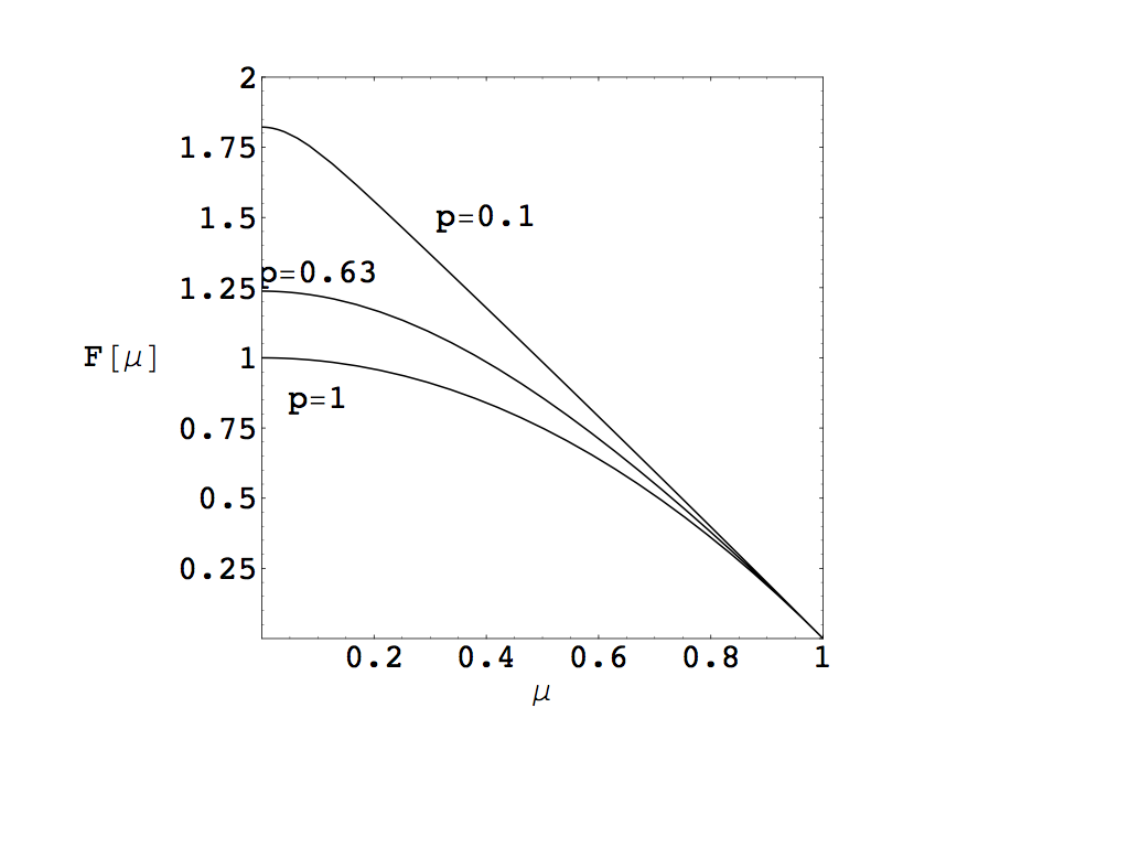
Figure 1: Function $F(\mu)$ for different values of $p$. For $p=0$, $F=2(1-\mu)$ almost everywhere except close to $\mu=0$ point, see Appendix A

Figure 2: Function $p(C)$. The extremum is at $C=0.87$, $p=0.63$. Dashed line is a small twist approximation (Eq. (14))

Figure 3: The net twist angle between two poles versus current parameter $C$. Dotted line is the small current limit (Eq. (14))

As the current increases the distribution of the poloidal magnetic flux evolves towards more spherical configuration, becoming isotropic in the limit $p=0$ (Fig. 4). At the same time the distribution of a radial current at the surface evolves from an approximately isotropic to strongly concentrated near equator for small $p$. The field lines become more twisted, but for small $p\rightarrow 0$ the twist is confined to narrow layers near the equator, while the rest of the field lines have little twist and also are straitened out (as compared with dipole) in the radial direction. A given field line has largest twist where it is furthest from the star - at the equator.

The radial dependence of the magnetic field softens to ${\bf B}\propto r^{-2.87}$ when $\Delta\phi_{\rm N-S}=1$ radian. The net twist approaches $\Delta\phi_{\rm N-S}=\pi$ (one-half turn) in the split monopole limit ($p=0$). For comparison, a twisted quadrupole magnetic field expands to infinity after $1/\sqrt{3}$ turns (Lynden-Bell & Boily, 1994). In the limit $p=0$ the field structure approaches split monopole: $F=2(1-\mu)$, with field line straightened out in the radial direction, $B_{r}/B_{\ast}={\rm sign[\mu]}/\tilde{r}^{2}$, $B_{\theta}=0$ plus a current sheet in the equatorial plane which curries a surface current $g_{\phi}=2{B_{\ast}}c/(2\pi\tilde{r}^{2})$. The magnetic flux leaves the northern hemisphere and after reaching infinity returns to the southern hemisphere.

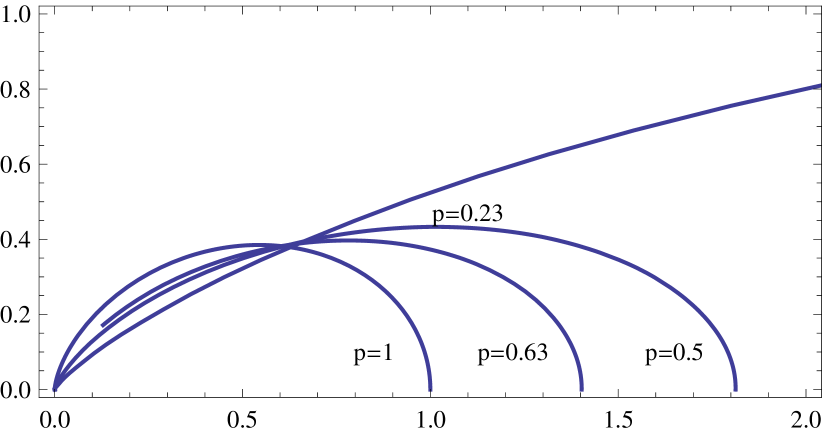
Figure 4: Form of the magnetic flux surfaces for different $p$; $p=1$ case corresponds to a dipole, $p=0$ is a monopole with radial poloidal fields.

The total current flowing through one hemisphere at radius $\tilde{r}$ is given by integral of $j_{r}$,

$$I={8\pi^{2}eB_{\ast}r_{\ast}\over c}\,\sqrt{Cp\over p+1}\,{1\over\tilde{r}^{p}}\,F(0)^{(p+1)/p)}.$$ (12)

Thus, a current that reaches to radius $\tilde{r}$ for a given twist decreases as $1/\tilde{r}^{p}$. On the other hand, the current flowing through the star (at $\tilde{r}=1$) increases continuously with decreasing $p$ and reaches $I_{\rm max}=8pi^{2}B_{\ast}r_{\ast}/c$ in the limit $p\rightarrow 0$. In fact, in this limit both northern (outgoing) and southern (ingoing) poloidal currents are confined to the equatorial plane and eliminate each other, leaving only toroidal current.

For small twists we can solve Eq. (5) analytically by expanding near $p=1,\,C=0$ and $F=1-\mu^{2}$. We find then $p=1-8C/35$ and

$$F=(1-\mu^{2})\left(1+{1\over 140}(1-\mu^{2})(17-5\mu^{2})C\right)$$ (13)

In this approximation flux function $\alpha$, magnetic field components and twist angle are given by

$$\alpha={\sqrt{2C}(1-\mu^{2})\over\tilde{r}}\mbox{}$$

$${B_{r}\over B_{\ast}}={\mu\over\tilde{r}^{3-8C/35}}\,\left(1+{3(13-18\mu^{2}+5\mu^{4})C\over 140}\right)\mbox{}$$

$${B_{\theta}\over B_{\ast}}={\sqrt{1-\mu^{2}}\over 2\tilde{r}^{3-8C/35}}\,\left(1-{(15+22\mu^{2}-5\mu^{4})C\over 1400}\right)\mbox{}$$

$${B_{\phi}\over B_{\ast}}={\sqrt{C}(1-\mu^{2})^{3/2}\over\sqrt{2}\tilde{r}^{2}}\mbox{}$$

$$\Delta\phi=\sqrt{2C}\mu$$ (14)

These relations are useful for the order of magnitude estimates. For example, for small twists the total poloidal current $I\sim\sin^{4}\theta/\tilde{r}$ is concentrated near the equator.

The simple twisted self-similar magnetosphere described above is not a temporal sequence, but, importantly, it provides simple and clear order-of-magnitude estimates of the effects involved. Numerical solutions (Parfrey et al., 2012) are in a general agreement with analytical estimates.

4 Variations of the spin-down rate

4.1 The CME model of magnetar bursts

The processes that cause magnetar X-ray flares (and possibly the persistent emission) may be similar to those operating in the Solar corona. The electric currents within the start are slowly pushed into the magnetosphere, gated by slow, plastic deformations of the neutron star crust. This leads to gradual twisting of the magnetospheric field lines, on time scales much longer than flares or burst, and creates active magnetospheric regions similar to Sun’s spots. Solutions described in Section 3 have energy stored in the magnetosphere that exceeds the energy of the dipolar configuration, Fig. 5, so that the dissipation of the supporting currents can power the magnetar high energy activity. Initially, when the electric current (and possibly magnetic flux) is pushed from the star into magnetosphere, the latter slowly adjusts to the changing boundary conditions. As more and more current is pushed into the magnetosphere it eventually reaches a point of dynamical instability beyond which the stable equilibrium can no longer be maintained. The loss of stability leads to a rapid restructuring of magnetic configuration, on the Alfvén crossing time scale, formation of narrow current sheets, and onset of magnetic dissipation. As a result, a large amount of magnetic energy is converted into the bulk motion kinetic energy and radiation. Moreover, the change of magnetic topology allows formation of expanding magnetic loops that eventually break away from the star (Lyutikov, 2006; Gourgouliatos & Lynden-Bell, 2008).

Figure 5: Energy contained in magnetosphere, compared with pure dipole field

Adapting the the generally accepted magnetic breakout model of Solar Coronal Mass Ejections (Lynch et al., 2008) to magnetar environment, the underlying cause of all the manifestations of Solar activity - CMEs, eruptive flares and filament ejections - is the disruption of a force balance between the upward pressure of the strongly sheared field of a filament channel and the downward tension of a potential (non-current carrying) overlying field. Thus, an eruption is driven solely by magnetic free energy stored in a closed, sheared magnetic fields that open toward infinity during an eruption. Reconnection is thought to plays a critical role in opening of magnetic field  lines: it removes the unsheared field above the low-lying, sheared core flux, thereby allowing this core flux to burst open.

4.2 The magnetospheric “anti-glitch”

Next we estimate parameter of the rapid spindown during an $X$-ray flare. Using the Goldrecih-Julian model, the spindown luminosity is related to the open magnetic flux $\Phi$: $L_{sd}\approx\Phi^{2}\Omega^{2}/c$. In particular, for dipole magnetosphere, $\Phi\approx B_{NS}R_{NS}^{2}(\Omega R_{NS}/c)$. In the twisted magnetosphere the open flux is larger (Thompson et al., 2002), so that the spin-down rate is

$$L_{sd}\sim B^{2}_{\ast}R_{\ast}^{2}c\left({\Omega R_{\ast}\over c}\right)^{2(p+1)},\,0<p<1$$ (15)

Thus,

$$\dot{\Omega}\propto\Omega^{2p+1},\,n=2p+1,1<n<3$$ (16)

where $n$ is the spindown index.

The changes of the magnetospheric structure can naturally induce large changes in the spindown rate. For example, for a given surface magnetic field $B$ and pulsar spin frequency $\Omega$, the maximal theoretical spindown rate (corresponding to the monopolar fields, $p=0,\,n=1$) is

$$\dot{\Omega}_{max}=\eta_{d}^{-2}\dot{\Omega}_{d}=10^{9}\dot{\Omega}_{d}\mbox{}$$

$$\eta_{d}={\Omega r_{\ast}\over c}\mbox{}$$

$$\dot{\Omega}_{d}\sim{B_{NS}^{2}R_{NS}^{2}c\over I_{NS}\Omega}\left({\Omega R_{\ast}\over c}\right)^{4}$$ (17)

where $\dot{\Omega}_{d}$ is a dipole spindown rate, $R_{NS}$ is neutron star radius, $B_{NS}$ is surface magnetic field, $I_{NS}$ is the moment of inertia and the numerical estimate is given for the particular magnetar. Thus, in long period neutron stars a relatively small change in the magnetospheric structure can induce huge variations in the spindown rate. This is due to the fact that in a dipolar-type configuration only a tiny fraction of the field lines, of the order of $\eta_{d}\sim 3\times 10^{-5}$ contributes to the spindown. A change in the fraction of the open flux then can induce large fluctuations of the spindown rate.

Let us assume that the persistent spindown rate $\dot{\nu}_{0}\approx-10^{-14}$ Hz/s (Archibald et al., 2013) is determined mostly by the dipolar-like spindown. Let the open magnetic flux during the outburst be a fraction $\eta$ of the total flux, so that the spindown rate is a faction $\eta^{2}$ of the maximal value (17), $\dot{\Omega}=\eta^{2}\dot{\Omega}_{max}$. Then to produce an “anti-glitch” of the order of $5\times 10^{-8}$ Hz within one period it is required that the fraction of the open flux is

$$\eta\approx\left({\Omega R_{\ast}\over c}\right)\sqrt{{\Delta\nu\over\dot{\nu}_{0}P}}=2.5\times 10^{-2}$$ (18)

Thus, all that is required to produce an “anti-glitch” is to open only a few percent of the total magnetic flux through hemisphere. Or, in other words, the enhanced torque should be of the order of $10^{-4}-10^{-5}$ of the maximal possible torque acting during one rotational period. For longer active spindown periods, the requirement on $\eta$ is even smaller. These are very reasonable estimates. The amount of open magnetic flux during the flare is much larger than for dipole field, $\eta\gg\eta_{d}$, yet it is much smaller than the total magnetic flux through a hemisphere, $\eta\ll 1$. Using numerical simulations of the twisted magnetosphere (Parfrey et al., 2012) came to similar conclusions, that opening a small fraction of the magnetosphere can lead to rapid spindown. The total energy involved in the opening of the magnetosphere  is a fraction $\sim\eta^{2}$ of the total magnetic field energy. In case of 1E 2259+586 (magnetic field of $6\times 10^{13}$ G) this amounts to $\sim 10^{41}$ ergs. This is consistent with the energy released in the prompt GBM burst, $\sim 10^{37}$ erg, after accounting for the radiative efficiency of the resulting CME-like event. We conclude that the “anti-glitch” behavior can be naturally explained as a transient high spindown rate induced by the magnetospheric changes.

4.3 Enhanced spindown and spectral hardening during $X$ activity

Immediately following the $X$-ray burst, the magnetar 1E 2259+586 showed a period of enhanced activity during which the spindown rate was approximately 2-3 times higher than the average value. Below we show this this is due to a mild overall increase in the magnetospheric current. Let us use the analytical small current approximation (14). In the self-similar model, for not very large twists, we have $p=1-8/35C,\,C=\Delta\phi^{2}/2$. If magnetospheric structure changes (e.g., there is a jump in the current parameter $\Delta C$ due to increased twist), this will induce a jump in the spin-down parameter $\Delta p=-8/35\Delta C$ and a corresponding jump in spin-down rate.

Let us assume that in a normal state a typical twist is $\Delta\phi_{0}$. As discussed above, it is required that spindown increased by a factor ${\cal N}\approx 2$ during the post burst phase. This requires that during the activity time

$$\Delta\phi^{2}=\Delta\phi_{0}^{2}+{35\over 16}{\ln{\cal N}\over\ln R_{LC}/r_{\ast}}$$ (19)

Assuming $\Delta\phi^{2}\gg\Delta\phi_{0}^{2}$ and using the parameters of the magnetar and the required spin-down increase, we find

$$\Delta\phi\approx 0.37$$ (20)

This is a reasonable estimate: during the activity time (a weeks after the $X$-ray flare in 1E 2259+586) the magnetosphere on average should be twisted by about twenty degrees. Note, that for large twists the spindown rate is a highly sensitive function of the twist: for a twenty degrees turn the spindown rate is 2 times the dipole, while for a full turn it is $10^{9}$ times the dipole, Eq. (17). Using the estimate of the twist, and the small current solutions (14), we find for the current parameter $C=0.06$ and $p=.98$, all within the assumed limit.

The fact that the twist (20) is smaller than unity is important for the self-consistency of the model. It is expected that highly twisted configurations are unstable towards kinks or buckling instabilities. Understanding stability of the configurations (6) remains an open question.

Note, that the spindown of a neutron star on long time scales (much longer than the period) are not uniquely related to the $X$-ray activity. The luminosity presumable comes from a large fraction of the magnetosphere, mostly from closed field lines. At the same time, the spindown is determined by currents flowing along a very small bundle of field lines. Thus we do not expect an exact one-to-one correspondence between the $X$-ray luminosity and the spindown rate, only a positive correlation.

On the other hand, suppose that the crustal motion twists a patch of the surface by a given angle. Twisting the flux tube originating near the magnetic pole and extending nearly up to the light cylinder is more likely to lead to kink insatiability and opening of the magnetosphere, since the instability of twisted closed field lines is likely to be suppressed by the overlying dipolar fields. But twisting the fields near the magnetic pole strongly affects the current responsible for the spindown of the star. Thus, it is natural to expect that a burst or a flares lead to temporary opening of the magnetosphere and large increase in the torque.

Lyutikov & Gavriil (2006) (see also Fernández & Thompson, 2007; Rea et al., 2008; Beloborodov, 2013) have constructed a model of resonant cyclotron scattering in the magnetar magnetospheres that relates the spindown properties to the hardness of the soft non-thermal radiation. According to the model, during the enhanced activity the magnetosphere typically supports larger currents. Larger currents and larger particle density in the magnetosphere increases the importance of resonant scattering, making the spectra harder. The optical depth due to resonant scattering $\tau$ can be expressed in terms of the current parameter $C$. For not very large twists

$$\tau\sim\sqrt{C}\propto\Delta\phi$$ (21)

(assuming a constant velocity of scatters). The resulting spectrum is not a pure power law, but is in agreement with the data. Qualitatively, the higher is the twist, the larger is the luminosity (see Eq. (34) of Thompson et al., 2002), the harder is the spectrum.

The total dissipated energy is proportional to the current (and the twist), $L_{X}\propto\Delta\phi$, so that $\tau\propto L_{X}$. Thus we expect that a substantial (order of unity) change in the $X$-ray luminosity is accompanied by a similar change in the spindown rate and a change in the spectral properties. All these relations are in agreement with the observations of 1E 2259+586.

5 Discussion

In this paper we showed that the transient (lasting for just one period) opening of a relatively small fraction of the magnetosphere (a few percent) can explain the rapid spindown of the magnetar 1E 2259+586 observed by Archibald et al. (2013). We point out that in magnetars it is very easy to have large variations of the spin-down rate - the theoretical upper limit is an enhancement by a factor up to $\sim 10^{9}$. What is more, in the ensuing period of the enhanced activity the behavior of the $X$-ray luminosity, spindown rates and spectral behavior are all consistent with the magnetospheric origin. We suggest, there may be no real second glitch, only erratic behavior while the magnetosphere relaxes to a long term steady state.

Magnetars are also known for their erratic timing behavior (e.g., Woods & Thompson, 2006). The spindown rates can vary by a factor of few over timescales of weeks (eg Woods et al., 2002), while the giant flares are often accompanied by a sudden increase in the spin period (Woods et al., 1999). Note that in case of magnetars the time “resolution” - a typical interval between the measurements of the spin, are about a week. This, combined with the fact that torque can fluctuate by as much as billion times, make it hard to define a glitch - as opposed to smooth torque variation.

In this paper we argue that timing fluctuations in magnetars are purely magnetospheric. (In contrast, Thompson et al., 2000, argued that large timing irregularities in magnetars may have an internal origin, similar to glitches in rotationally powered pulsars.). We suggest that there are two types of glitches in magnetars: (i) due to topological changes of the magnetosphere - opening up of a considerable magnetic flux (rapid spin down on the time scale of one rotation, associated with some radiative activity; this is specific to magnetars); (ii) smooth changes in the magnetospheric structure (radiatively silent, no large $X$-ray bursts, spindown changes can be positive or negative; this is similar to the torque variations in the rotationally powered pulsars). In the second case there is a clear prediction: larger averaged $L_{X}$, larger spindown, harder spectra (this is generally consistent with the behavior of 1E 2259+586, as well as post-giant flare evolution, see discussion in Lyutikov (2006)). The first case (opening up of the magnetosphere) leads to transient spindown events during bursts and flares and is specific to magnetars, while the second case (changes in the current flow in the magnetosphere), produces fluctuations around some mean value and is analogues to torque fluctuations in rotationally-powered pulsar.

In comparison, in the rotationally powered pulsars there are two types of timing irregularities: glitches, sudden changes of the spin frequency occurring on the time scale of single rotation period (e.g., Espinoza et al., 2011) and long term spindown variations (Kramer et al., 2006; Hermsen et al., 2013). Glitches are related to the internal neutron star dynamics, how the superfluid vortexes interact with the crustal lattice (Chamel & Haensel, 2008). The long term torque variations are assumed to be related to the changes in the magnetospheres current distribution, though a lack of general understanding of pulsar magnetospheres impede the development of models (see, though Timokhin & Arons, 2013). We suggest that the second type, magnetospheric long term variations, is also operational in magnetars, though generally with larger spin variations. Magnetars also have new specific torque variation mechanism due to opening of the magnetosphere.

We hypothesize that in cases of so called spin-up glitches, the “prompt” short spike, like the one detected by the GBM in 1E 2259+586, was missed by the all sky monitors. Then the ensuing erratic behavior of the spin-down torque can lead to overcompensation of the prompt spin-down glitch.

As we discuss next, the overall timing behavior of magnetars is in a general agreement with the magnetospheric model. Dib & Kaspi (in preparation) point out that radiative changes are almost always accompanied by some form of timing anomaly - in our model the magnetospheric opening is accompanied by a formation of a CME and associated prompt spike. Also, large long term magnetospheric changes should have correlated spindown and persistent $X$-ray flux increase. On the other hand, only occasionally timing anomalies in AXPs are accompanied by any form of radiative anomaly. Most of the torque variations in our model come from the magnetospheric changes on the closed field lines - such changes are not necessarily expected to be associated with large radiative effects. Importantly, the changes in the magnetospheric structure of closed field lines should show in the changing pulse profiles. This agrees with observations.

Superficially, the timing glitches in normal pulsars and magnetars look similar: roughly same amplitude, similar recovery and inter-glitch times (about a day or so). We think these similarities are misleading. For example, the rate of accumulation of any mismatch between different components within the neutron star, $\propto\Omega^{3}$, is different by an order of a million between the glitching pulsars (which are typically fast) and the slow magnetars.

There are other possible hints in favor of the magnetospheric origin of magnetar timing anomalies. The magnetar 1E 1048.1-5937 has the highest rotational noise, has one of the largest flux variations and has the highest surface temperature (Dib & Kaspi, in preparation). This is also consistent with the magnetospheric model: larger variations of the current are related to large flux and spindown variations. The high surface temperature is related to higher overall magnetospheric currents. In addition, the timing noise is correlated with the strength of the magnetic field: 1E 2259+586 and 4U 0142+61 have the least noise and smallest magnetic field, while 1RXS J1708-4009 and 1E 1841-045 are the opposite.

Finally, there are magnetar activity events that seem to be associated with spin-up glitches (e.g., the 2007 event in 1E 1048.1-5937, Dib et al., 2009). We note that at the time of the event there were very large variations in $\dot{\Omega}$, that, we hypothesize, when averaged over the interval between the observations produced an effective spin-up event.

I would like to thank Robert Archibald, Andrei Beloborodov, Konstantinos Gourgouliatos, Victoria Kaspi, Christopher Thompson and David Tsang for discussions and Department of Physics of McGill University for hospitality. This research was partially supported by NASA grant NNX12AF92G and by Simons Foundation.

Appendix A $p\rightarrow 0$ limit

Interesting analytical approximations can be obtained in the limit $p\rightarrow 0$. In this case function $F$ is almost a straight line with a slope $-2$ everywhere except near the point $\mu=0$ with $F(0)\sim 2$. Near this point we can neglect $\mu^{2}$. Integrating Eq. (5) once we find

$$p(p+1)F^{2}+{Cp\over p+1}F^{2(p+1)/p}+{F^{\prime}}^{2}=4$$ (A1)

where constant of integration has been chose so that at $\mu=1$, where $F=0$, ${F^{\prime}}^{2}=4$. Since at $\mu\rightarrow 0$ the function $F\sim 2$ is raised to a large power we can neglect the term $p(p+1)F$ as compared with $CF^{(p+2)/p}$:

$${Cp\over p+1}F^{2(p+1)/p}+{F^{\prime}}^{2}=4$$ (A2)

Making a substitution

$$F\rightarrow\left({pC\over 4(p+1)}\right)^{-{p\over 2(p+1)}}\left(1-{p\over p+1}\ln q\right)\equiv{2(p+1)\over C_{2}p}\left(1-{p\over p+1}\ln q\right),$$ (A3)

the equation for the function $q$ reads

$${q^{\prime}\over\sqrt{q^{2}-1}}=C_{2}$$ (A4)

where

$$C_{2}=\left({2(p+1)\over p}\right)^{1/(p+1)}\left({C(p+1)\over p}\right)^{p/(2(p+1))}$$ (A5)

Boundary conditions for $q$ are

$$1-{p\over p+1}\ln q=0 \mu=1$$ at (A6)

$$q^{\prime}=0 \mu=0$$ at

(two boundary conditions for the first order ODE (A4) are needed to find the solution and dependence $p(C)$). Eq. (A4) has a solution

$$q=\cosh(C_{2}\mu+C_{1})$$ (A7)

Boundary conditions give

$$C_{1}=0$$

$$C_{2}=\cosh^{-1}\exp^{(p+1)/p}\sim(p+1)/p+\ln 2$$ (A8)

which resolves implicitly $p(C)$

$$C={2^{-2/p}(p+1)\over p}$$ (A9)

and determines the flux function

$$F={2\over\cosh^{-1}\exp^{(p+1)/p}}\,\left({p+1\over p}-\ln\cosh(\mu\cosh^{-1}\exp^{(p+1)/p})\right)\mbox{}$$

$$\sim{2(p+1)\over 1+p+p\ln 2}\left(1-{p\over p+1}\ln\cosh\mu(1+1/p+\ln 2)\right).$$ (A10)

(compare with Lynden-Bell & Boily, 1994). Value of $F$ at $\mu=0$ is then

$$F(0)={2(p+1)\over 1+p+p\ln 2}\sim 2(1-p\ln 2)$$ (A11)

References

- Archibald et al. (2013) Archibald, R. F., Kaspi, V. M., Ng, C.-Y., Gourgouliatos, K. N., Tsang, D., Scholz, P., Beardmore, A. P., Gehrels, N., & Kennea, J. A. 2013, Nature, 497, 591
- Beloborodov (2013) Beloborodov, A. M. 2013, ApJ, 762, 13
- Chamel & Haensel (2008) Chamel, N. & Haensel, P. 2008, Living Reviews in Relativity, 11, 10
- Dib et al. (2009) Dib, R., Kaspi, V. M., & Gavriil, F. P. 2009, ApJ, 702, 614
- Espinoza et al. (2011) Espinoza, C. M., Lyne, A. G., Stappers, B. W., & Kramer, M. 2011, MNRAS, 414, 1679
- Fernández & Thompson (2007) Fernández, R. & Thompson, C. 2007, ApJ, 660, 615
- Forbes et al. (2006) Forbes, T. G., Linker, J. A., Chen, J., Cid, C., Kóta, J., Lee, M. A., Mann, G., Mikić, Z., Potgieter, M. S., Schmidt, J. M., Siscoe, G. L., Vainio, R., Antiochos, S. K., & Riley, P. 2006, Space Science Reviews, 123, 251
- Gourgouliatos (2008) Gourgouliatos, K. N. 2008, MNRAS, 385, 875
- Gourgouliatos & Lynden-Bell (2008) Gourgouliatos, K. N. & Lynden-Bell, D. 2008, MNRAS, 391, 268
- Hermsen et al. (2013) Hermsen, W., Hessels, J. W. T., Kuiper, L., van Leeuwen, J., Mitra, D., de Plaa, J., Rankin, J. M., Stappers, B. W., Wright, G. A. E., Basu, R., Alexov, A., Coenen, T., Grießmeier, J.-M., Hassall, T. E., Karastergiou, A., Keane, E., Kondratiev, V. I., Kramer, M., Kuniyoshi, M., Noutsos, A., Serylak, M., Pilia, M., Sobey, C., Weltevrede, P., Zagkouris, K., Asgekar, A., Avruch, I. M., Batejat, F., Bell, M. E., Bell, M. R., Bentum, M. J., Bernardi, G., Best, P., Bîrzan, L., Bonafede, A., Breitling, F., Broderick, J., Brüggen, M., Butcher, H. R., Ciardi, B., Duscha, S., Eislöffel, J., Falcke, H., Fender, R., Ferrari, C., Frieswijk, W., Garrett, M. A., de Gasperin, F., de Geus, E., Gunst, A. W., Heald, G., Hoeft, M., Horneffer, A., Iacobelli, M., Kuper, G., Maat, P., Macario, G., Markoff, S., McKean, J. P., Mevius, M., Miller-Jones, J. C. A., Morganti, R., Munk, H., Orrú, E., Paas, H., Pandey-Pommier, M., Pandey, V. N., Pizzo, R., Polatidis, A. G., Rawlings, S., Reich, W., Röttgering, H., Scaife, A. M. M., Schoenmakers, A., Shulevski, A., Sluman, J., Steinmetz, M., Tagger, M., Tang, Y., Tasse, C., ter Veen, S., Vermeulen, R., van de Brink, R. H., van Weeren, R. J., Wijers, R. A. M. J., Wise, M. W., Wucknitz, O., Yatawatta, S., & Zarka, P. 2013, Science, 339, 436
- Horowitz et al. (2011) Horowitz, C. J., Hughto, J., Schneider, A., & Berry, D. K. 2011, ArXiv e-prints
- Jones (2003) Jones, P. B. 2003, ApJ, 595, 342
- Komissarov et al. (2007) Komissarov, S. S., Barkov, M., & Lyutikov, M. 2007, MNRAS, 374, 415
- Kramer et al. (2006) Kramer, M., Lyne, A. G., O’Brien, J. T., Jordan, C. A., & Lorimer, D. R. 2006, Science, 312, 549
- Lynch et al. (2008) Lynch, B. J., Antiochos, S. K., DeVore, C. R., Luhmann, J. G., & Zurbuchen, T. H. 2008, ApJ, 683, 1192
- Lynden-Bell & Boily (1994) Lynden-Bell, D. & Boily, C. 1994, MNRAS, 267, 146
- Lyutikov (2003) Lyutikov, M. 2003, MNRAS, 346, 540
- Lyutikov (2006) —. 2006, MNRAS, 367, 1594
- Lyutikov & Gavriil (2006) Lyutikov, M. & Gavriil, F. P. 2006, MNRAS, 368, 690
- Palmer et al. (2005) Palmer, D. M., Barthelmy, S., Gehrels, N., Kippen, R. M., Cayton, T., Kouveliotou, C., Eichler, D., Wijers, R. A. M. J., Woods, P. M., Granot, J., Lyubarsky, Y. E., Ramirez-Ruiz, E., Barbier, L., Chester, M., Cummings, J., Fenimore, E. E., Finger, M. H., Gaensler, B. M., Hullinger, D., Krimm, H., Markwardt, C. B., Nousek, J. A., Parsons, A., Patel, S., Sakamoto, T., Sato, G., Suzuki, M., & Tueller, J. 2005, Nature, 434, 1107
- Parfrey et al. (2012) Parfrey, K., Beloborodov, A. M., & Hui, L. 2012, ApJ, 754, L12
- Pavan et al. (2009) Pavan, L., Turolla, R., Zane, S., & Nobili, L. 2009, MNRAS, 395, 753
- Rea et al. (2008) Rea, N., Zane, S., Turolla, R., Lyutikov, M., & Götz, D. 2008, ApJ, 686, 1245
- Shafranov (1966) Shafranov, V. D. 1966, Reviews of Plasma Physics, 2, 103
- Thompson & Duncan (1995) Thompson, C. & Duncan, R. C. 1995, MNRAS, 275, 255
- Thompson et al. (2000) Thompson, C., Duncan, R. C., Woods, P. M., Kouveliotou, C., Finger, M. H., & van Paradijs, J. 2000, ApJ, 543, 340
- Thompson et al. (2002) Thompson, C., Lyutikov, M., & Kulkarni, S. R. 2002, ApJ, 574, 332
- Timokhin & Arons (2013) Timokhin, A. N. & Arons, J. 2013, MNRAS, 429, 20
- Wolfson (1995) Wolfson, R. 1995, ApJ, 443, 810
- Woods et al. (2002) Woods, P. M., Kouveliotou, C., Gövgüş, E., Finger, M. H., Swank, J., Markwardt, C. B., Hurley, K., & van der Klis, M. 2002, ApJ, 576, 381
- Woods et al. (1999) Woods, P. M., Kouveliotou, C., van Paradijs, J., Finger, M. H., Thompson, C., Duncan, R. C., Hurley, K., Strohmayer, T., Swank, J., & Murakami, T. 1999, ApJ, 524, L55
- Woods & Thompson (2006) Woods, P. M. & Thompson, C. Soft gamma repeaters and anomalous X-ray pulsars: magnetar candidates, ed. W. H. G. Lewin & M. van der Klis, 547–586