arXiv:1306.XXX

Abstract

Superconformal methods are useful to build invariant actions in supergravity. We have a good insight in the possibilities of actions that are at most quadratic in spacetime derivatives, but insight in general higher-derivative actions is missing. Recently higher-derivative actions got more attention for several applications. One of these is the understanding of finiteness of loop computations in supergravities. Divergences can only occur if invariant counterterms or anomalies exist. One can wonder whether conformal symmetry might also play a role in this context. In order to construct higher-derivative supergravities with the conformal methods, one should first get more insight in such rigid supersymmetric actions with extra fermionic symmetries. We show how Dirac–Born–Infeld actions with Volkov–Akulov supersymmetries can be constructed in all orders.

 Contribution to the proceedings of ’Breaking of supersymmetry and Ultraviolet Divergences in extended Supergravity’, Frascati, March 2013, to be published as Springer Lecture Notes
e-mail: Antoine.VanProeyen@fys.kuleuven.be

0.1 Introduction

In the last 35 years, supergravity actions with terms that are at most quadratic in spacetime derivatives have been studied a lot. But recently higher-derivative terms in supergravity actions got more interest. There are different reasons for this. They appear as order $\alpha^{\prime}$ terms in the effective action of string theory. It has also been realized that they lead to corrections to the black hole entropy. Furthermore, they can give higher order results in the AdS/CFT correspondence. In this talk, we will also consider them as counterterms for UV divergences of quantum loops.

In Sect. 0.2, we will review what we know about general sugra (supergravity) and susy (supersymmetry) theories. Our preferred method to obtain such theories uses the superconformal method, which we review in Sect. 0.3. We will also discuss there in which sugra theories these can be used. Then, in Sect. 0.4 we will turn to higher-derivative sugra actions and explain the relation with sugra loop results. We will see that we miss a lot of insight in the possibilities for higher-derivative actions. In view of this, we studied Dirac–Born–Infeld actions for vector multiplets, obtaining closed expressions and exhibiting extra Volkov–Akulov type supersymmetries. They are examples of all order higher-derivative susy actions. They are the deformation of the well-known lowest order supersymmetry action, and can be considered also perturbatively in a bottom-up construction. We will summarize this result in Sect. 0.5, before giving conclusions in Sect. 0.6.

0.2 General sugra/susy theories

An overview of possible actions with supersymmetry and supergravity has been given in chapter 12 of the book Freedman:2012zz , starting from the basics. The theories considered there are ‘ordinary’ supersymmetry and supergravity theories, which means that the bosonic terms in the action are at most quadratic in spacetime derivatives, while the terms with fermions are at most linear in spacetime derivatives. In 4 dimensions they typically contain the frame field $e_{\mu}^{a}$, gauge fields $A_{\mu}^{A}$, with field strengths $F^{A}_{\mu\nu}$, scalars $\varphi^{u}$, gravitinos $\psi_{\mu}^{i}$, and spin-1/2 fermions $\lambda^{m}$ and a Lagrangian of the form

$$e^{-1}{\cal L} = {\textstyle\frac{1}{2}}R+{\textstyle\frac{1}{4}}(\mathop{\rm Im}\nolimits{{\cal N}_{AB}})F^{A}_{\mu\nu}F^{\mu\nu B}-{\textstyle\frac{1}{8}}(\mathop{\rm Re}\nolimits{{\cal N}_{AB}})e^{-1}\varepsilon^{\mu\nu\rho\sigma}F^{A}_{\mu\nu}F^{B}_{\rho\sigma}$$ (1)

$$-{\textstyle\frac{1}{2}}g_{uv}D_{\mu}\varphi^{u}D^{\mu}\varphi^{v}-V(\varphi)$$

$$\left\{-{\textstyle\frac{1}{2}}\bar{\psi}_{\mu i}\gamma^{\mu\nu\rho}D_{\nu}\psi_{\rho}{}^{i}-{\textstyle\frac{1}{2}}g_{A}{}^{B}\bar{\lambda}^{A}\not{D}\lambda_{B}+\textrm{h.c.}\right\}+\ldots\,,$$

where ${\cal N}_{AB}$, $g_{uv}$ and $g_{A}{}^{B}$ are functions of the scalars $\varphi$. In general, the possibilities for susy theories depend on the properties of irreducible spinors in each dimension. For theories with Minkowski signature, these can be summarised in Table 1.

Table 1: Irreducible spinors, number of components and symmetry properties.

dim	spinor	min # components
2	MW	1
3	M	2
4	M	4
5	S	8
6	SW	8
7	S	16
8	M	16
9	M	16
10	MW	16
11	M	32

For each spacetime dimension it is indicated whether Majorana (M), Majorana–Weyl (MW), symplectic (S) or symplectic Weyl (SW) spinors can be defined as the ‘minimal spinor’, and the number of real components of this minimal spinor is given. To make a complete list, we further use the information of what is the maximal number of susy generators in such theories. This is based on an analysis of representations of susy in 4 dimensions, which leads to maximal ${\cal N}=8$ for sugra, and maximal ${\cal N}=4$ for susy. This thus translates to maximal 32 real generators for sugra and 16 for susy. This information is based on an analysis of particle states i.e. states with momentum, spin and helicity $|p^{\mu},s,h\rangle$. One needs that susy generators transform a boson state to a fermion state and that they square to translations, which is an invertible operator. Considering these operators as acting from bosonic states to fermionic states or the inverse, leads to the conclusion that there are an equal number of bosonic and fermionic states (number of degrees of freedom), and to the possible particle representations Strathdee:1987jr . The information of the maximal number of susy generators can also be used in dimensions higher than 4, since any higher-dimensional theory can be reduced on tori to $D=4$, keeping the same number of susy generators. We recalled the essential elements of the proofs here, in order to distinguish supersymmetries of this kind, to the Volkov–Akulov supersymmetries. The latter do not transform between such bosonic and fermionic states and should thus not be included in the relevant counting of the number of supersymmetry generators. Using this information leads to Table 2.

Table 2: Supersymmetry and supergravity theories in dimensions 4 to 11.

$\begin{array}[]{| *{11}{c|} }D&\mbox{SUSY}&\lx@intercol\hfil 32\hfil\lx@intercol\vrule\lx@intercol&24&20&\lx@intercol\hfil 16\hfil\lx@intercol\vrule\lx@intercol&12&8&4\\ \hline\cr 11&\mathrm{M}&M&&&&\lx@intercol\hfil\hfil\lx@intercol\vrule\lx@intercol&&&\\ 10&\mathrm{MW}&\mathrm{IIA}&\mathrm{IIB}&&&\begin{array}[]{c}I\\ \phantom{{\cal N}}\heartsuit\\ \end{array}&&&&\\ 9&\mathrm{M}&\lx@intercol\hfil{\cal N}=2\hfil\lx@intercol\vrule\lx@intercol&&&\begin{array}[]{c}{\cal N}=1\\ \phantom{{\cal N}}\heartsuit\\ \end{array}&&&&\\ 8&\mathrm{M}&\lx@intercol\hfil{\cal N}=2\hfil\lx@intercol\vrule\lx@intercol&&&\begin{array}[]{c}{\cal N}=1\\ \phantom{{\cal N}}\heartsuit\\ \end{array}&&&&\\ 7&\mathrm{S}&\lx@intercol\hfil{\cal N}=4\hfil\lx@intercol\vrule\lx@intercol&&&\begin{array}[]{c}{\cal N}=2\\ \phantom{{\cal N}}\heartsuit\\ \end{array}&&&&\\ 6&\mathrm{SW}&\lx@intercol\hfil(2,2)\hfil\lx@intercol\vrule\lx@intercol&(2,1)&&\begin{array}[]{c}(1,1)\\ \phantom{{\cal N}}\heartsuit\\ \end{array}&\begin{array}[]{c}(2,0)\\ \phantom{{\cal N}}\diamondsuit\\ \end{array}&&\begin{array}[]{c}(1,0)\\ \heartsuit,\diamondsuit,\clubsuit\\ \end{array}&\\ 5&\mathrm{S}&\lx@intercol\hfil{\cal N}=8\hfil\lx@intercol\vrule\lx@intercol&{\cal N}=6&&\lx@intercol\hfil\begin{array}[]{c}{\cal N}=4\\ \phantom{{\cal N}}\heartsuit\\ \end{array}\hfil\lx@intercol\vrule\lx@intercol&&\begin{array}[]{c}{\cal N}=2\\ \phantom{{\cal N}}\heartsuit,\clubsuit\\ \end{array}&\\ 4&M&\lx@intercol\hfil{\cal N}=8\hfil\lx@intercol\vrule\lx@intercol&{\cal N}=6&{\cal N}=5&\lx@intercol\hfil\begin{array}[]{c}{\cal N}=4\\ \phantom{{\cal N}}\heartsuit\\ \end{array}\hfil\lx@intercol\vrule\lx@intercol&\begin{array}[]{c}{\cal N}=3\\ \phantom{{\cal N}}\heartsuit\\ \end{array}&\begin{array}[]{c}{\cal N}=2\\ \heartsuit,\clubsuit\\ \end{array}&\begin{array}[]{c}{\cal N}=1\\ \heartsuit,\clubsuit\\ \end{array}\\ \hline\cr\vrule\lx@intercol\hfil\hfil\lx@intercol\vrule\lx@intercol&\lx@intercol\hfil\mathrm{SG}\hfil\lx@intercol\vrule\lx@intercol&\lx@intercol\hfil\mathrm{SG/SUSY}\hfil\lx@intercol\vrule\lx@intercol&\mathrm{SG}&\lx@intercol\hfil\mathrm{SG/SUSY}\hfil\lx@intercol\vrule\lx@intercol\\ \end{array}$

An entry in the table represents the possibility to have supergravity theories in a specific dimension $D$ with the number of (real) supersymmetries indicated in the top row. We first repeat for every dimension the type of spinors that can be used. Theories with up to 16 (real) supersymmetry generators allow ‘matter’ multiplets. Considering the on-shell states of the free theories we distinguish different kinds of such multiplets. Those that contain a gauge field $A_{\mu}$ are called vector multiplets or gauge multiplets, and are indicated in Table 2 with $\heartsuit$. Tensor multiplets in $D=\hbox{6}$ contain an antisymmetric tensor $T_{\mu\nu}$, are are indicated by $\diamondsuit$. Multiplets with only scalars and spin-1/2 fields are indicated with $\clubsuit$. They are the hypermultiplets in case of 8 supersymmetry generators, or the Wess–Zumino chiral multiplets for ${\cal N}=1$, $D=4$. At the bottom is indicated whether these theories exist only in supergravity (SG), or also with just global supersymmetry (SUSY).

For each entry in the Table there are basic supergravities and ‘deformations’. Basic supergravities have only gauged supersymmetry and general coordinate transformations (and U(1) s of vector fields). There is no potential for the scalars, and there are only Minkowski vacua. A deformation means that, without changing the kinetic terms of the fields, the couplings are changed. Many deformations are gauged supergravities . That means that a Yang–Mills group is gauged, introducing a potential. Such supergravities are produced by fluxes on branes in string theory. There are also other deformations (e.g. massive deformations, the superpotential in ${\cal N}=1$ supersymmetry, …).

The embedding tensor formalism offers a way to classify the gauged supergravities. It defines the gauge group as a subgroup of the isometry group G, as can be seen from the covariant derivative $\left(\partial_{\mu}-A_{\mu}{}^{M}\Theta_{M}{}^{\alpha}\delta_{\alpha}\right)\phi$. Here, $\alpha$ labels all the rigid symmetries, while $M$ labels those that are gauged. The ‘embedding tensor’ $\Theta_{M}{}^{\alpha}$ determines which symmetries are gauged and in which amount they contribute. E.g. the coupling constants are part of this tensor. The tensor should satisfy a number of constraints, whose solutions determine the possible gaugings Cordaro:1998tx ; Nicolai:2001sv ; deWit:2005ub . This thus allows to get a complete picture of supergravities with at most two spacetime derivatives in Lagrangian, though it still needs more work to get all the explicit solutions of the constraints.

For higher-derivative actions there is no such systematic knowledge. There are various constructions of higher derivative terms, e.g. using supersymmetric Dirac–Born–Infeld actions, but there is no systematic construction or classification of possibilities; certainly not for supergravity, but even not for supersymmetry.

0.3 The superconformal method

There are various ways to construct supergravity actions. A basic way is the order-by-order Noether method: starting from a globally symmetric action, next order terms in the gravitational coupling constant are added using the concepts of Noether currents. This is in fact the only possibility for the theories with more than 16 susy generators. The superspace method is very useful for rigid ${\cal N}=1$ supersymmetry. However, it becomes very difficult for supergravity. One needs many fields and many gauge transformations to get to a supergravity action. There is also the (super)group manifold approach, where optimal use is made of the symmetries using constraints on the curvatures. We adhere to the method of superconformal tensor calculus whenever possible. This method has the advantage that it uses the nice features of superspace, like the the structure of multiplets, but it avoids its immense number of unphysical degrees of freedom. The extra symmetries that are used in this method often lead to insight in the structure of a supergravity theory.

Superconformal symmetry is the maximal extension of spacetime symmetries according to the Coleman–Mandula theorem. What we have in mind, is not the construction of the supersymmetric completion of Weyl gravity, $\int{\rm d}^{4}x\sqrt{g}\left[R_{\mu\nu\rho\sigma}^{2}-2R_{\mu\nu}^{2}+{\textstyle\frac{1}{3}}R^{2}\right]$, but the construction of Poincaré gravity,

$$S_{\rm Poinc}=\int{\rm d}^{4}x\,\frac{1}{2\kappa^{2}}\sqrt{g}\,R\,,$$ (2)

using conformal methods, where the dimensionful gravitational coupling constant $\kappa$ signals a breaking of the conformal symmetry. Thus, we use the conformal symmetry as a tool for the construction of actions. It allows us to use multiplet calculus similar to superspace, and it makes hidden symmetries explicit.

We first explain the strategy for the construction of pure gravity in a conformal way. One starts with a conformal coupling of a scalar field, which will act as ‘compensator’:

$${\cal L}=-{\textstyle\frac{1}{2}}\sqrt{g}\,\phi\,\Box^{C}\phi=-{\textstyle\frac{1}{2}}\sqrt{g}\,\phi\Box\phi+{\textstyle\frac{1}{12}}\sqrt{g}\,R\phi^{2}\,.$$ (3)

This action has local scale transformations $\delta\phi(x)=\lambda_{\rm D}(x)\phi(x)$. These can be gauge-fixed by choosing a value

$$\phi=\sqrt{6}/\kappa\,.$$ (4)

This introduces the scale $\kappa$, indicating the breaking of conformal symmetry. Using (4) in (3) leads to (2). The mechanism thus starts with a conformal invariant action, and has a Poincaré invariant action as a result after gauge fixing. This is systematically indicated in Table 3.

Table 3: Conformal construction of Poincaré gravity

Conformal gauge multiplet coupled to a scalar heelveelzever  local conformal

⇓ gauge fix non-conformal symmetries

conformalPoincaré gravity local Poincaré symmetry

For the supersymmetric theories, a similar construction allows to get more insight in the structure of supergravity actions. A main difference between supersymmetry and supergravity is that multiplets have a clear structure in supersymmetry, but after coupling to supergravity they often get mixed, and they are not clearly identifiable in the final action. In another language: superfields are an easy conceptual tool for globally supersymmetric theories. With the similar method as described above for gravity, supergravity can also be obtained by starting with an action with superconformal symmetry and gauge fixing the superfluous symmetries. This is especially useful for matter-coupled supergravities. Before the gauge fixing, everything looks like in global supersymmetry, just adding covariantizations for the superconformal symmetries. Only after the gauge fixing, the multiplets get mixed.

To elucidate the superconformal symmetry, it is useful to consider it in the way of transformations of supermatrices of the form

$$\pmatrix{\mbox{conformal algebra}&Q,S\cr Q,S&R\mbox{-symmetry}}\,.$$ (5)

$Q$ is the ordinary supersymmetry and $S$ is the extra, ‘special’ supersymmetry. The $R$-symmetry depends on the dimension and extension of supersymmetry. It is clarifying to order the generators according to their weight under dilatations (here for the ${\cal N}=1$ superconformal algebra)

$$1 : P_{a}$$

$${\textstyle\frac{1}{2}} : Q$$

$$0 : D\,,\ M_{ab}\,,\ T$$

$$-{\textstyle\frac{1}{2}} : S$$

$$-1 : K_{a}\,.$$ (6)

$P_{a}$, $D$, $M_{ab}$ and $K_{a}$ are the conformal generators. The $R$-symmetry is in this case just U(1), whose generator is indicated by $T$. The weights in the first column of (6) determine the commutators involving $D$, for example

$$[D,Q]={\textstyle\frac{1}{2}}Q\,,\qquad[D,S]=-{\textstyle\frac{1}{2}}S\,.$$ (7)

As we discussed above, $T$ is an $R$-symmetry. All (anti)commutators are consistent with the weights, e.g.

$$\left\{Q_{\alpha},Q^{\beta}\right\}=-{\textstyle\frac{1}{2}}(\gamma^{a})_{\alpha}{}^{\beta}P_{a}\,,\qquad\left\{S_{\alpha},S^{\beta}\right\}=-{\textstyle\frac{1}{2}}(\gamma^{a})_{\alpha}{}^{\beta}K_{a}\,,$$

$$\left\{Q_{\alpha},S^{\beta}\right\}=-{\textstyle\frac{1}{2}}\delta_{\alpha}{}^{\beta}D-{\textstyle\frac{1}{4}}(\gamma^{ab})_{\alpha}{}^{\beta}M_{ab}+{\textstyle\frac{1}{2}}{\rm i}(\gamma_{*})_{\alpha}{}^{\beta}T\,.$$ (8)

The strategy for the superconformal construction of ${\cal N}=1$ supergravity is analogous as for gravity in Table 3. It is depicted in Table 4

Table 4: Superconformal construction of pure ${\cal N}=1$ supergravity

heelveelzever Superconformal gauge multiplet (${\cal N}=1$ Weyl multiplet) coupled to a chiral multiplet

superChiral multiplet  ⇓  gauge fix dilatations, special conformal transformations, local U(1)-symmetry and special supersymmetry

superconformal gaupure ${\cal N}=1$ supergravity

A similar scheme holds for ${\cal N}=4$ supergravity Bergshoeff:1981is ; deRoo:1984gd as shown in Table 5.

Table 5: Superconformal construction of pure ${\cal N}=4$ supergravity

heelveelzever Superconformal gauge multiplet (${\cal N}=4$ Weyl multiplet) coupled to 6 gauge compensating multiplets (on-shell)

superChiral multiplet  ⇓  gauge fix dilatations, special conformal transformations, local SU(4), local U(1) and special supersymmetry

superconformal gaupure ${\cal N}=4$ Cremmer-Scherk-Ferrara supergravity

The special feature is that the gauge compensating multiplets are on-shell multiplets. Remember that in any case the action should be invariant without use of the field equations, but the algebra of the symmetries may close only modulo field equations. However, the problem is that in this way there is no flexibility in the field equations. They are already fixed by the supersymmetry transformation laws. This gives thus a problem when we want to modify the action with higher-derivative terms, since then the field equations will change. Therefore, higher-derivative terms cannot be added to ${\cal N}=4$ supergravity without a modification of the field equations. The hypermultiplets of ${\cal N}=2$ supergravity already have this feature of an ‘on-shell algebra’ (at least for a generic hyper-Kähler manifold). The ${\cal N}=4$ gauge multiplets also share this property. This is especially relevant since they are compensating multiplets. It implies that the supersymmetry transformations of the ${\cal N}=4$ super-Poincaré theory can only close modulo field equations. But one can apply the superconformal method.

In which supergravity theories can we use the superconformal methods ? There are two necessary ingredients. First, one should have a superconformal algebra. Second, there should be compensating multiplets. Which theories allow superconformal algebras was already analysed by W. Nahm Nahm:1978tg . He analysed in which simple superalgebras the conformal algebra $\mathop{\mathfrak{so}}(D,2)$ is a factor in the bosonic subalgebra. This lead to Table 6 (also a long list of superconformal algebras exist for $D=2$).

Table 6: Superconformal algebras

$D$	supergroup	conf	$R$	ferm.
$3$	$\mathop{\rm OSp}(N|4)$	$\mathop{\rm SO}(3,2)=\mathop{\rm Sp}(4)\$	$\mathop{\rm SO}(N)$	$4N$
$4$	$\mathop{\rm SU}(2,2|N)$	$\mathop{\rm SO}(4,2)=\mathop{\rm SU}(2,2)$	$\mathop{\rm{}U}(N)$ for $N\neq 4$	$8N$
			$\mathop{\rm SU}(4)$ for $N=4$
$5$	$F^{2}(4)$	$\mathop{\rm SO}(5,2)$	$\mathop{\rm SU}(2)$	16
$6$	$\mathop{\rm OSp}(8^{*}|2N)$	$\mathop{\rm SO}(6,2)=\mathop{\rm SO}^{*}(8)$	$\mathop{\rm USp}(2N)$	$16N$

In each case the bosonic subgroup contains the covering group of $\mathop{\rm SO}(D,2)$, such that spinor representations are possible, and a compact $R$-symmetry group. The last column gives the number of real supersymmetry generators. Other superconformal algebras have been considered where the conformal algebra is not a factor, but still a subalgebra of the bosonic part of the superalgebra. E.g. $\mathop{\rm SO}(11,2)\subset\mathop{\rm Sp}(64)\subset\mathop{\rm OSp}(1|64)$ vanHolten:1982mx ; D'Auria:2000ec . However, these have not been successfully applied for constructing actions. Thus, the superconformal methods are restricted to the dimensions and extensions that appear in Table 6 and furthermore to a number of supersymmetries $\leq 16$, such that compensating multiplets exist. This leads to those indicated in boxes in Table 7.

Table 7: Supergravity theories for which superconformal methods can be used

$\begin{array}[]{| *{11}{c|} }D&\mbox{SUSY}&\lx@intercol\hfil 32\hfil\lx@intercol\vrule\lx@intercol&24&20&\lx@intercol\hfil 16\hfil\lx@intercol\vrule\lx@intercol&12&8&4\\ \hline\cr 11&\mathrm{M}&M&&&&\lx@intercol\hfil\hfil\lx@intercol\vrule\lx@intercol&&&\\ 10&\mathrm{MW}&\mathrm{IIA}&\mathrm{IIB}&&&I&&&&\\ 9&\mathrm{M}&\lx@intercol\hfil{\cal N}=2\hfil\lx@intercol\vrule\lx@intercol&&&{\cal N}=1&&&&\\ 8&M&\lx@intercol\hfil{\cal N}=2\hfil\lx@intercol\vrule\lx@intercol&&&{\cal N}=1&&&&\\ 7&S&\lx@intercol\hfil{\cal N}=4\hfil\lx@intercol\vrule\lx@intercol&&&{\cal N}=2&&&&\\ 6&SW&\lx@intercol\hfil(2,2)\hfil\lx@intercol\vrule\lx@intercol&(2,1)&&(1,1)&\ \framebox{(2,0)}&&\ \framebox{(1,0)}&\\ 5&S&\lx@intercol\hfil{\cal N}=8\hfil\lx@intercol\vrule\lx@intercol&{\cal N}=6&&\lx@intercol\hfil{\cal N}=4\hfil\lx@intercol\vrule\lx@intercol&&\ \framebox{${\cal N}=2$}&\\ 4&M&\lx@intercol\hfil{\cal N}=8\hfil\lx@intercol\vrule\lx@intercol&{\cal N}=6&{\cal N}=5&\lx@intercol\hfil\ \framebox{${\cal N}=4$}\hfil\lx@intercol\vrule\lx@intercol&\ \framebox{${\cal N}=3$}&\ \framebox{${\cal N}=2$}&\ \framebox{${\cal N}=1$}\\ \hline\cr\end{array}$

0.4 Higher derivative sugra actions and sugra loop results

For many years it was believed that supergravity could not be a finite theory. However, since the calculations of Bern:2007hh revealed the 3-loop finiteness of ${\cal N}=8$, $D=4$ supergravity, we realize that quantum supergravity has more surprising features than we understood so far. In Bern:2009kd the result was extended to 4 loops and even to $D=5$. But then, also ${\cal N}=4$ supergravity in $D=4$ turned out to be finite up to 3 loops Bern:2012cd (and further results followed for $D=5$). This brings us to reflections on the nature of supergravity and possible counterterms. Divergences would imply that supersymmetric counterterms should exist (or there should be supersymmetric anomalies). But our present knowledge on higher-derivative terms in supergravity is not sufficient to be sure about which invariants can be consistently defined.

0.4.1 Superconformal methods for the ${\cal N}=2$ example

Superconformal methods have been used to construct higher-derivative supergravities, starting with the work of S. Cecotti and S. Ferrara Cecotti:1986gb . Especially for ${\cal N}=2$ supergravity, the tensor calculus allows us to construct various terms deWit:2010za . The constructions use tensor calculus with chiral multiplets, which are similar to chiral superfields. The multiplets contain fields

$$S=\{X,\Omega_{i},\ldots,C\}\,.$$ (9)

Any sum and product of these gives another chiral multiplets. These manipulations allow ‘tensor calculus’. A useful tool is the kinetic multiplet of a chiral multiplet (which is also chiral) and starts with the complex conjugate of the highest component of a chiral multiplet:

$$\mathbb{T}(\bar{S})=\{\bar{C},\ldots\}\,.$$ (10)

To construct higher-derivative terms, one needs also another chiral multiplet, formed from the ${\cal N}=2$ Weyl multiplet

$$W^{2}=\{T_{ab}^{-}T^{ab\,-},\ldots\}\,.$$ (11)

It starts from the square of an auxiliary field (antisymmetric tensor) of the Weyl multiplet. One can then use tensor calculus on these multiplets to construct new chiral multiplets, of which the highest components defines actions. In order to be able to define these in the superconformal framework, one has to take into account the dilatation symmetry. This implies that the function of chiral multiplets that is used to construct actions should satisfy homogeneity properties. Using such homogeneous functions of the chiral multiplets, one obtains supergravity theories using superconformal covariantization of the expressions used for global supersymmetry. Hence this leads to many possibilities, which are invariants contributing to the entropy and central charges of black holes.

In order to see how these actions lead to DBI theories, $R^{4}$ actions are considered in Chemissany:2012pf , using the above-mentioned constructions with

$$\left[S^{2}+\lambda\frac{W^{2}}{S^{2}}\mathbb{T}\left(\frac{\bar{W}^{2}}{\bar{S}^{2}}\right)\right]_{C}\,.$$ (12)

It uses the action formula ‘$C$’, which means in global supersymmetry the highest component of th chiral multiplet. In superconformal calculus, there are some correction terms involving the gravitino, to obtain local conformal symmetry. $S$ is the chiral compensating multiplet (which due to constraints is in fact a vector multiplet). Using just the first term in (12) would lead to pure supergravity. The second term in (12) uses the multiplet (11) and the construction of a kinetic multiplet (10). The powers of $S$ are chosen in order to satisfy the homogeneity properties leading to conformal-invariant actions. That second term is taken with a coupling constant $\lambda$, in which an expansion will be considered.

Apart from a term of the form $\lambda C_{\cdot\cdot\cdot\cdot}^{4}$, where $C_{\cdot\cdot\cdot\cdot}$ is the Weyl tensor, and thus creating terms of the form $R^{4}$, the action formula in (12) produces also terms of the type $\lambda(\partial T)^{4}$, where $T$ stands for the auxiliary field of the Weyl multiplet. In the standard supergravity action, the field equations imply that $T$ is on-shell proportional to the graviphoton. For the action (12), we get, symbolically

$$T_{ab}=\frac{2}{X}F_{ab}+\lambda(\partial^{4}T^{3})_{ab}\,,$$ (13)

where $X$ is the scalar of the compensating multiplet, which is in the Poincaré theory dependent on $\kappa$ similar to (4). This equation is solved recursively, and we thus get an expression with an infinite number of higher derivative terms with higher and higher powers of the graviphoton $F$:

$$T_{ab}=\frac{2}{X}F_{ab}+\lambda(\partial^{4}F^{3})_{ab}+\lambda^{2}\partial^{4}F^{2}\partial^{4}F^{3}+\ldots\,.$$ (14)

The action with auxiliary field eliminated leads to a DBI-type action with higher derivatives

$$S_{\rm deformed}=-{\textstyle\frac{1}{4}}F^{2}+\lambda(\partial F)^{4}+\lambda^{2}\partial^{8}F^{6}+\ldots\,.$$ (15)

Note that before the elimination of the auxiliary field, this action has a finite number of terms with auxiliary fields. The infinite series is produced by the elimination of the auxiliary fields. They lead thus to a deformation of the lowest order action in powers of $\lambda$. At the same time also the transformation laws are deformed. Again, the transformation laws are finite expressions before the elimination of the auxiliary fields. E.g. for the gravitino transformation

$$\delta\psi_{\mu}^{i}=D_{\mu}\epsilon^{i}-{\textstyle\frac{1}{16}}\gamma^{ab}T_{ab}^{-}\varepsilon^{ij}\gamma_{\mu}\epsilon_{j}-\gamma_{\mu}\eta^{i}\,,$$ (16)

where the covariant derivative uses the superconformal connections, and $S$-supersymmetry with parameter $\eta^{i}$ is included. Then the on-shell value of the auxiliary fields is used as a power series in $\lambda$:

$$\phi_{\rm aux}=\phi^{(0)}_{\rm aux}+\Delta\phi_{\rm aux}\,,\qquad\Delta\phi_{\rm aux}=\sum_{n=1}\lambda^{n}\phi^{(n)}_{\rm aux}\,.$$ (17)

This leads, with (14), to deformations in the supersymmetry transformation law of the gravitino of the form Chemissany:2012pf

$$\Delta\psi_{\mu}^{i}=-4\lambda[\partial^{4}F^{3}]_{\mu}{}^{\nu}\gamma_{\nu}\epsilon^{i}+\ldots\,.$$ (18)

Here also contributions have been used that originate from the ‘decomposition law’ expressing the parameter $\eta^{i}$ in terms of $\epsilon^{i}$ after gauge fixing of $S$-supersymmetry.

We conclude that the tensor calculus allows us to obtain higher-derivative terms, determined first off-shell, which can lead to deformations of the action and transformation laws on-shell. They are obtained from (broken) superconformal actions. For pure gravity, the 3-loop counterterm that contains $R^{4}$ is obtained from the local conformal expression

$$\int{\rm d}^{4}\sqrt{g}\,\phi^{-4}(C_{\mu\nu\rho\sigma}C^{\mu\nu\rho\sigma})^{2}\,,$$ (19)

where $\phi$ is the compensating scalar and $C_{\mu\nu\rho\sigma}$ is the Weyl tensor. For ${\cal N}=2$ a superconformal $R^{4}$ counterterm can be obtained from the $\lambda$-term in (12). What do we know about ${\cal N}=4$, where miraculous cancelations have been found?

0.4.2 Problem and conjecture for ${\cal N}=4$ supergravity

The problem is that it is not easy to construct counterterms for ${\cal N}=4$ supergravity. We cannot multiply the compensating multiplets to suitable powers, and thus we cannot make constructions as those for ${\cal N}=2$. The essential problem is that the algebra of supersymmetry holds only on shell. When we would like to write a modified action, then it implies modified field equations, and thus the transformations have to be modified (or in other words: the structure of the multiplets). For ${\cal N}=2$, deformed transformations could be found due to the possibility to work first with auxiliary fields. The field equations for the latter lead to deformed transformation laws on shell. For ${\cal N}=4$ we do not know auxiliary fields. How can we then establish the the existence or non-existence of the consistent order by order deformation of ${\cal N}=4$ supergravity?

This question lead to the conjecture made in Ferrara:2012ui . If such counterterms do not exist, this may explain finiteness results (if meanwhile the explicit calculations do not find that ${\cal N}=4$, $D=4$ is divergent at higher loops). Until invariant counterterms are constructed we have no reason to expect UV divergences. We can also conjecture that such counterterms should be broken superconformal expressions, if conformal symmetry is more than a classical symmetry. Thus there are two points of view. The first one is that legitimate counterterms are not available yet, and we still have to construct them. The second one is that legitimate counterterms are not available, and cannot be constructed, offering an explanation of finiteness.

In fact, if the UV finiteness will persist in higher loops, one would like to view this as an opportunity to test some new ideas about gravity. One possible idea is that superconformal symmetry, used in the classical theory as a tool to construct actions, is more fundamental and has also a quantum significance. As mentioned in Sect. 0.3, the classical theory can be obtained from gauge fixing a superconformal action. In that way, the Planck mass appears only in the gauge-fixing procedure. This looks analogous to the appearance of the masses of $W$ and $Z$ vector mesons in the standard model. They are not present in the gauge-invariant action, and show up when the gauge symmetry is spontaneously broken. In the unitary gauge these masses give the impression of being fundamental. In the renormalizable gauge, where the UV properties are analysed, they are absent. One may hope that a similar understanding can be obtained in the future to give a more fundamental significance to the superconformal symmetry. The possible non-existence of (broken) superconformal-invariant counterterms and anomalies in ${\cal N}=4$, $D=4$ supergravity could then explain the miraculous results of the quantum calculations.

Such ideas would give a simple explanation of the 3-loop finiteness and predict perturbative UV finiteness in higher loops. The same conjecture applies to higher-derivative superconformal invariants and to the existence of a consistent superconformal anomaly. Also for the latter, one may either say that we still have to understand how to construct such an anomaly, or maybe it does not exist. Therefore, the conjecture is economical, sparing in the use of resources: either the local ${\cal N}=4$ superconformal symmetry is a good symmetry, or it is not. The conjecture is falsifiable by the ${\cal N}=4$ 4-loop computations (which are already underway, as we heard during the conference). If the conjecture survives these computations (if they show further UV finiteness), then this gives a further hint that the models with superconformal symmetry serve as a basis for constructing a consistent quantum theory where the Planck mass appears only in the process of gauge fixing the superconformal symmetry. However, it is also falsifiable by our own calculations: if we find a way to construct (non-perturbative) superconformal invariants that can serve as counterterms, then this conjecture is circumvented. We will start to search in that direction, following a quote of R. Feynman: “We are trying to prove ourselves wrong as quickly as possible, because only in that way can we find progress.”

0.5 Dirac–Born–Infeld - Volkov–Akulov and deformation of supersymmetry

The main problem for the superconformal construction of counterterms in ${\cal N}=4$ supergravity is thus that the compensating multiplets have only been defined with transformations that close on-shell using the field equations of the 2-derivative action. These compensating multiplets are vector multiplets. In our recent work Bergshoeff:2013pia we search for deformations of vector multiplet actions such that higher-derivative terms occur. We will find all-order higher derivative globally supersymmetric invariant actions. They are of the Dirac–Born–Infeld (DBI) type, and have extra symmetries, of Volkov–Akulov (VA) type. The latter are not yet $S$-supersymmetry transformations that we would like in the context of the superconformal programme mentioned above, but we will comment on this at the end.

We will consider vector multiplets with a gauge vector and a spinor field. We want that the supersymmetry algebra is closed, but not necessary off-shell, since the main problems that we want to address are theories with only an on-shell closed algebra. A gauge vector in $D$ dimensions has $D-2$ on-shell degrees of freedom, while a spin-1/2 fermion has on-shell half the number of degrees of freedom of the number of components of the spinor. Considering Table 1 shows that one can have an equal number of bosonic and fermionic degrees of freedom for these fields in the cases $D=10$ with Majorana–Weyl spinors, $D=6$ with symplectic Majorana–Weyl spinors, $D=4$ with Majorana spinors, and even $D=3$ with Majorana spinors. Comparing with Table 2 shows that these are the maximal dimensions to have vector multiplets for supersymmetries with 16, 8, 4 and 2 generators. Other vector multiplets are obtained from these by dimensional reduction, which generates also scalar on-shell degrees of freedom.

These theories are described by an action of the form

$$S=\int{\rm d}^{D}x\,\big{\{}-{\textstyle\frac{1}{4}}(F_{\mu\nu})^{2}-{\textstyle\frac{1}{2}}\bar{\lambda}\not{\partial}\lambda\big{\}}\,.$$ (20)

They are invariant under supersymmetry transformations

$$\delta_{\epsilon}A_{\mu}=-{\textstyle\frac{1}{2}}{\bar{\epsilon}}\Gamma_{\mu}\lambda\,,\qquad\delta_{\epsilon}\lambda={\textstyle\frac{1}{4}}\Gamma^{\mu\nu}F_{\mu\nu}\epsilon\,,$$ (21)

where the spinors are of the appropriate type mentioned before, and for the case of symplectic Majorana-Weyl spinors also the extension index $i=1,2$ has been suppressed with the understanding that e.g.

$${\bar{\epsilon}}\Gamma_{\mu}\lambda={\bar{\epsilon}}^{i}\Gamma_{\mu}\lambda_{i}=\varepsilon^{ij}{\bar{\epsilon}}_{j}\Gamma_{\mu}\lambda_{i}\,.$$ (22)

The action has also an extra trivial (global) fermionic shift symmetry

$$\delta_{\eta}A_{\mu}=0\,,\qquad\delta_{\eta}\lambda=-{\textstyle\frac{1}{2\alpha}}\eta\,,$$ (23)

where the normalization with a constant $\alpha$ has been used in order to match with formulas that will follow below.

0.5.1 The bottom-up approach

We first attempt a ‘bottom-up’ approach. This means that we define a deformation of the action with terms proportional to a parameter $\alpha$, and adapt simultaneously the transformation laws. In this we follow Bergshoeff:1986jm , where this was considered for $D=6$, and an action was obtained of the form

$$S = \int{\rm d}^{D}x\,\big{\{}-{\textstyle\frac{1}{4}}F^{2}-{\textstyle\frac{1}{2}}\bar{\lambda}\not{\partial}\lambda\big{\}}+\alpha c_{4}F^{\mu\nu}\bar{\lambda}\Gamma_{\mu}\partial_{\nu}\lambda$$ (24)

$$+{\textstyle\frac{1}{8}}\alpha^{2}\Big{[}\mathop{\rm Tr}\nolimits F^{4}-{\textstyle\frac{1}{4}}\,\left(F^{2}\right)^{2}-2(1+4c_{4}^{2})\big{(}F^{2}\big{)}^{\mu\nu}\bar{\lambda}\Gamma_{\mu}\partial_{\nu}\lambda$$

$$-{\textstyle\frac{1}{2}}(1-4c_{4}^{2})F_{\mu}{}^{\lambda}\big{(}\partial_{\lambda}F_{\nu\rho}\big{)}\bar{\lambda}\Gamma^{\mu\nu\rho}\lambda-{\textstyle\frac{1}{4}}(c_{1}+8c_{4}^{2})F^{2}\bar{\lambda}\not{\partial}\lambda$$

$$+{\textstyle\frac{1}{4}}c_{2}F_{\mu\nu}\big{(}\partial_{\lambda}F^{\lambda}{}_{\rho}\big{)}\bar{\lambda}\Gamma^{\mu\nu\rho}\lambda+{\textstyle\frac{1}{4}}(c_{3}+4c_{4}^{2})F_{\mu\nu}F_{\rho\sigma}\bar{\lambda}\Gamma^{\mu\nu\rho\sigma}\not{\partial}\lambda\Big{]}$$

$$+{\cal O}(\alpha^{2}\lambda^{4})+{\cal O}(\alpha^{3})\,.$$

The parameters $\lambda_{i}$ are undetermined. However, they are all related to field redefinitions

$$A_{\mu}(0) = A_{\mu}+{\textstyle\frac{1}{32}}\alpha^{2}c_{2}F^{\nu\rho}\bar{\lambda}\Gamma_{\mu\nu\rho}\lambda\,,$$

$$\lambda(0) = \lambda+{\textstyle\frac{1}{2}}\alpha c_{4}F_{\mu\nu}\Gamma^{\mu\nu}\lambda+{\textstyle\frac{1}{32}}\alpha^{2}c_{1}F^{2}\lambda-{\textstyle\frac{1}{32}}\alpha^{2}c_{3}F_{\mu\nu}F_{\rho\sigma}\Gamma^{\mu\nu\rho\sigma}\lambda\,,$$ (25)

where on the right-hand side are the fields corresponding to $c_{i}=0$, and on the left-hand side those for arbitrary $c_{i}$. Hence, up to these redefinitions, the answer is unique up to this order. Remark e.g. that it contains in the bosonic part the unique combination

$$\mathop{\rm Tr}\nolimits F^{4}-{\textstyle\frac{1}{4}}\,\left(F^{2}\right)^{2}\,,\qquad\mathop{\rm Tr}\nolimits F^{4}\equiv F_{\mu\nu}F^{\nu\rho}F_{\rho\sigma}F^{\sigma\mu}\,,\qquad F^{2}=F_{\mu\nu}F^{\mu\nu}\,.$$ (26)

Also the transformation laws are deformed with respect to (21). As well ordinary supersymmetry transformations (parameter $\epsilon$) as the extra supersymmetry (23) can be defined. E.g. for the latter we have now

$$\delta_{\eta}A^{\mu} = -{\textstyle\frac{\alpha}{8}}\bar{\eta}F^{\nu\mu}\Gamma_{\nu}\lambda-{\textstyle\frac{\alpha}{16}}\bar{\eta}\Gamma^{\mu\nu\rho}F_{\nu\rho}\lambda+{\textstyle\frac{1}{32}}\alpha c_{2}F_{\nu\rho}\bar{\eta}\Gamma^{\mu\nu\rho}\lambda+{\cal O}(\alpha\eta\lambda^{3})+{\cal O}(\alpha^{2})\,,$$

$$\delta_{\eta}\lambda = -{\textstyle\frac{1}{2\alpha}}\eta+\alpha\left[-{\textstyle\frac{1}{32}}F^{2}-{\textstyle\frac{1}{64}}\Gamma^{\mu\nu\rho\sigma}F_{\mu\nu}F_{\rho\sigma}\right]\eta$$ (27)

$$+{\textstyle\frac{1}{4}}c_{4}F_{\mu\nu}(c)\Gamma^{\mu\nu}\left[\eta-{\textstyle\frac{1}{2}}\alpha c_{4}F_{\rho\sigma}(c)\Gamma^{\rho\sigma}\eta\right]$$

$$+{\textstyle\frac{1}{64}}\alpha c_{1}F^{2}\eta-{\textstyle\frac{1}{64}}\alpha c_{3}F_{\mu\nu}F_{\rho\sigma}\Gamma^{\mu\nu\rho\sigma}\eta+{\cal O}(\alpha\eta\lambda^{2})+{\cal O}(\alpha^{2})\,.$$

It turns out that we can write this for all $D=10,6,4,3$ with the appropriate spinors types (Majorana, Majorana–Weyl, symplectic Majorana–Weyl) as mentioned above . The only spinor properties that we need are the Majorana flip relations, like

$$\bar{\lambda}_{1}\Gamma^{\mu}\lambda_{2}=-\bar{\lambda}_{2}\Gamma^{\mu}\lambda_{1}\,,\qquad\bar{\lambda}_{1}\Gamma^{\mu\nu\rho}\lambda_{2}=\bar{\lambda}_{2}\Gamma^{\mu\nu\rho}\lambda_{1}\,,$$ (28)

and the cyclic Fierz identity

$$\Gamma_{\mu}\lambda_{1}\bar{\lambda}_{2}\Gamma^{\mu}\lambda_{3}+\Gamma_{\mu}\lambda_{2}\bar{\lambda}_{3}\Gamma^{\mu}\lambda_{1}+\Gamma_{\mu}\lambda_{3}\bar{\lambda}_{1}\Gamma^{\mu}\lambda_{2}=0\,.$$ (29)

These are valid for all these cases. Note that all bilinears in spinors contain odd-rank gamma matrices, as is consistent with the fact that the spinors are all of the same chirality in $D=10$ and $D=6$. But this property holds also for e.g. $D=4$.

The results look very complicated and it seems hopeless to continue this to all orders in $\alpha$ and adding higher order spinor terms.

0.5.2 The top-down approach

We Bergshoeff:2013pia found a solution to the problem of the construction of the infinite series of deformations starting from the $\kappa$-symmetric action for D$p$ branes. This action is of the form

$$S_{\rm DBI}+S_{\rm WZ}=-\frac{1}{\alpha^{2}}\int{\rm d}^{p+1}\sigma\,\sqrt{-\det(G_{\mu\nu}+\alpha{\cal F}_{\mu\nu})}+\frac{1}{\alpha^{2}}\int\Omega_{p+1}\,,$$ (30)

where the first term is a DBI action, and $\kappa$-supersymmetry implies that it should be complemented with a Wess–Zumino (WZ) term in terms of an appropriate $(p+1)$-form $\Omega_{p+1}$ (see e.g. (45) in Aganagic:1996nn ). In the DBI term appear

$$G_{\mu\nu}\equiv\eta_{mn}\Pi_{\mu}^{m}\Pi_{\nu}^{n}\ ,\qquad\Pi_{\mu}^{m}\equiv\partial_{\mu}X^{m}+{\textstyle\frac{1}{2}}\bar{\theta}\Gamma^{m}\partial_{\mu}\theta\,,$$

$${\cal F}_{\mu\nu}\equiv F_{\mu\nu}+\alpha^{-1}\bar{\theta}\sigma_{3}\Gamma_{m}\partial_{[\mu}\theta\left(\partial_{\nu]}X^{m}+{\textstyle\frac{1}{4}}\bar{\theta}\Gamma^{m}\partial_{\nu]}\theta\right)\,.$$ (31)

We consider these actions in the context of the IIB theory, and thus $X^{m}$ with $m=0,\ldots,9$ denote the spacetime coordinates of the $D=10$ theory. The coordinates on the brane are indicated by $\mu=0,\ldots,p$, and $p$ should be odd. $\theta$ is a doublet of Majorana–Weyl spinors, of which we omit again the extension index. $F_{\mu\nu}$ is an Abelian field strength.

This action has the following symmetries. First, there is a rigid supersymmetry doublet parameter $\epsilon^{1}$, $\epsilon^{2}$. There is also rigid Poincaré symmetry in $D=10$. Furthermore, there are local symmetries on the brane. On the bosonic side these are the worldvolume general coordinate transformations. Furthermore there is the $\kappa$-supersymmetry doublet. Effectively only half of these are present, since they this is a reducible symmetry, which means that it appears only in the form

$$\delta_{\kappa}\theta=(1+\Gamma)\kappa\,,$$ (32)

where $\Gamma$ is a matrix such that $(1+\Gamma)$ is a projection on half of the spinor space.

Though this has been obtained from IIB superstring theory in $D=10$, it turns out that the action (30) has also the same symmetries when we consider $D=6$, just changing the index range to $m=0,\ldots,5$ and using symplectic Majorana–Weyl spinors. This implies that we consider the $(2,0)$ theory in the $D=6$, 16 supersymmetries entry of Table 2. This theory is often called iib. The action has then also a brane interpretation, (using again odd $p$) Bergshoeff:2012jb as has been clarified in the talk of E. Bergshoeff in this conference. Moreover, we can also consider it solutions of $D=4$, ${\cal N}=2$ supergravity with worldvolume action as in (30) (thus $m=0,\ldots,3$ and $p=3$ or 1).

We then gauge-fix local symmetries imposing for a $p$-brane (describing here the embedding in $D=10$, but the other cases are obtained by changing the range of indices)

$$X^{m}=\{\delta^{m^{\prime}}_{\mu}\sigma^{\mu},\phi^{I}\}\,,\quad m^{\prime}=0,1,\dots,p\,,\quad I=1,\dots,9-p$$

$$\theta=(\theta^{1}=0,\,\theta^{2}\equiv\alpha\lambda)\,.$$ (33)

The first line fixes the worldvolume general coordinate transformations by identifying the coordinates in the embedding spacetime with the worldvolume coordinates. This leaves $9-p$ scalars. In the second line, the effective $\kappa$-symmetry is fixed, and the remaining coordinate is renamed $\lambda$ in order to make the connection with the down-up approach. These gauges lead to decomposition laws, implying that the parameters of the worldvolume general coordinate transformations and $\kappa$-symmetry become functions of the remaining (global) symmetries. There are thus two, deformed, fermionic symmetries $\epsilon^{1}$ and $\epsilon^{2}$. Two combinations of these symmetries are called $\epsilon$ and $\zeta$, and can be related to the $\epsilon$ and $\eta$ symmetries of the bottom-up approach.

We first consider the action for the case $p=9$ in this gauge, which reduces (30) to

$$S=-\frac{1}{\alpha^{2}}\int{\rm d}^{10}x\,\left\{\sqrt{-\det(G_{\mu\nu}+\alpha{\cal F}_{\mu\nu})}-1\right\}\,,$$ (34)

where

$$G_{\mu\nu}=\eta_{mn}\Pi_{\mu}^{m}\Pi_{\nu}^{n}\ ,\qquad\Pi_{\mu}^{m}=\delta_{\mu}^{m}+{\textstyle\frac{1}{2}}\alpha^{2}\bar{\lambda}\Gamma^{m}\partial_{\mu}\lambda\,,$$

$${\cal F}_{\mu\nu}\equiv F_{\mu\nu}-\alpha\bar{\lambda}\Gamma_{[\nu}\partial_{\mu]}\lambda\,,\qquad\mu=0,1,...,9\,,\qquad m=0,1,...,9\,.$$ (35)

This action possesses 16 $\epsilon$ transformations, which are deformations of the Maxwell supermultiplet supersymmetries:

$$\delta_{\epsilon}\lambda = -{\textstyle\frac{1}{2\alpha}}\left(\mathord{\!\leavevmode\hbox{ \begin{picture}(0.6,0.7)\put(0.0,0.0){\line(1,0){0.5}} \put(0.15,0.0){\line(0,1){0.7}} \put(0.35,0.0){\line(0,1){0.8}} \put(0.3,0.8){\rule{0.5pt}{0.5pt}}\put(0.26,0.78){\rule{0.5pt}{0.5pt}}\put(0.22,0.76){\rule{0.5pt}{0.5pt}}\put(0.18,0.74){\rule{0.5pt}{0.5pt}}\put(0.14,0.72){\rule{0.5pt}{0.5pt}}\put(0.1,0.7){\rule{0.5pt}{0.5pt}}\put(0.06,0.68){\rule{0.5pt}{0.5pt}}\put(0.02,0.66){\rule{0.5pt}{0.5pt}}\put(-0.02,0.64){\rule{0.5pt}{0.5pt}}\put(-0.06,0.62){\rule{0.5pt}{0.5pt}}\put(-0.1,0.6){\rule{0.5pt}{0.5pt}}\put(-0.14,0.58){\rule{0.5pt}{0.5pt}} \end{picture}}}-\beta\right)\epsilon+{\textstyle\frac{1}{4}}\alpha\partial_{\mu}\lambda\bar{\lambda}\Gamma^{\mu}\left(\mathord{\!\leavevmode\hbox{ \begin{picture}(0.6,0.7)\put(0.0,0.0){\line(1,0){0.5}} \put(0.15,0.0){\line(0,1){0.7}} \put(0.35,0.0){\line(0,1){0.8}} \put(0.3,0.8){\rule{0.5pt}{0.5pt}}\put(0.26,0.78){\rule{0.5pt}{0.5pt}}\put(0.22,0.76){\rule{0.5pt}{0.5pt}}\put(0.18,0.74){\rule{0.5pt}{0.5pt}}\put(0.14,0.72){\rule{0.5pt}{0.5pt}}\put(0.1,0.7){\rule{0.5pt}{0.5pt}}\put(0.06,0.68){\rule{0.5pt}{0.5pt}}\put(0.02,0.66){\rule{0.5pt}{0.5pt}}\put(-0.02,0.64){\rule{0.5pt}{0.5pt}}\put(-0.06,0.62){\rule{0.5pt}{0.5pt}}\put(-0.1,0.6){\rule{0.5pt}{0.5pt}}\put(-0.14,0.58){\rule{0.5pt}{0.5pt}} \end{picture}}}+\beta\right)\epsilon\,,$$

$$\delta_{\epsilon}A_{\mu} = {\textstyle\frac{1}{4}}\bar{\lambda}\Gamma_{\mu}\big{(}\mathord{\!\leavevmode\hbox{ \begin{picture}(0.6,0.7)\put(0.0,0.0){\line(1,0){0.5}} \put(0.15,0.0){\line(0,1){0.7}} \put(0.35,0.0){\line(0,1){0.8}} \put(0.3,0.8){\rule{0.5pt}{0.5pt}}\put(0.26,0.78){\rule{0.5pt}{0.5pt}}\put(0.22,0.76){\rule{0.5pt}{0.5pt}}\put(0.18,0.74){\rule{0.5pt}{0.5pt}}\put(0.14,0.72){\rule{0.5pt}{0.5pt}}\put(0.1,0.7){\rule{0.5pt}{0.5pt}}\put(0.06,0.68){\rule{0.5pt}{0.5pt}}\put(0.02,0.66){\rule{0.5pt}{0.5pt}}\put(-0.02,0.64){\rule{0.5pt}{0.5pt}}\put(-0.06,0.62){\rule{0.5pt}{0.5pt}}\put(-0.1,0.6){\rule{0.5pt}{0.5pt}}\put(-0.14,0.58){\rule{0.5pt}{0.5pt}} \end{picture}}}+\beta\big{)}\epsilon$$ (36)

$$+{\textstyle\frac{1}{8}}\alpha^{2}\bar{\lambda}\Gamma_{m}({\textstyle\frac{1}{3}}\mathord{\!\leavevmode\hbox{ \begin{picture}(0.6,0.7)\put(0.0,0.0){\line(1,0){0.5}} \put(0.15,0.0){\line(0,1){0.7}} \put(0.35,0.0){\line(0,1){0.8}} \put(0.3,0.8){\rule{0.5pt}{0.5pt}}\put(0.26,0.78){\rule{0.5pt}{0.5pt}}\put(0.22,0.76){\rule{0.5pt}{0.5pt}}\put(0.18,0.74){\rule{0.5pt}{0.5pt}}\put(0.14,0.72){\rule{0.5pt}{0.5pt}}\put(0.1,0.7){\rule{0.5pt}{0.5pt}}\put(0.06,0.68){\rule{0.5pt}{0.5pt}}\put(0.02,0.66){\rule{0.5pt}{0.5pt}}\put(-0.02,0.64){\rule{0.5pt}{0.5pt}}\put(-0.06,0.62){\rule{0.5pt}{0.5pt}}\put(-0.1,0.6){\rule{0.5pt}{0.5pt}}\put(-0.14,0.58){\rule{0.5pt}{0.5pt}} \end{picture}}}+\beta)\epsilon\bar{\lambda}\Gamma^{m}\partial_{\mu}\lambda+{\textstyle\frac{1}{4}}\alpha\bar{\lambda}\Gamma^{\rho}\left(\mathord{\!\leavevmode\hbox{ \begin{picture}(0.6,0.7)\put(0.0,0.0){\line(1,0){0.5}} \put(0.15,0.0){\line(0,1){0.7}} \put(0.35,0.0){\line(0,1){0.8}} \put(0.3,0.8){\rule{0.5pt}{0.5pt}}\put(0.26,0.78){\rule{0.5pt}{0.5pt}}\put(0.22,0.76){\rule{0.5pt}{0.5pt}}\put(0.18,0.74){\rule{0.5pt}{0.5pt}}\put(0.14,0.72){\rule{0.5pt}{0.5pt}}\put(0.1,0.7){\rule{0.5pt}{0.5pt}}\put(0.06,0.68){\rule{0.5pt}{0.5pt}}\put(0.02,0.66){\rule{0.5pt}{0.5pt}}\put(-0.02,0.64){\rule{0.5pt}{0.5pt}}\put(-0.06,0.62){\rule{0.5pt}{0.5pt}}\put(-0.1,0.6){\rule{0.5pt}{0.5pt}}\put(-0.14,0.58){\rule{0.5pt}{0.5pt}} \end{picture}}}+\beta\right)\epsilon F_{\rho\mu}\,,$$

where $\beta$ is a matrix ($\hat{\Gamma}^{\mu}=\Pi^{\mu}_{m}\Gamma^{m}$)

$$\beta = \left[\det\left(\delta_{\mu}{}^{\nu}+\alpha{\cal F}_{\mu\rho}G^{\rho\nu}\right)\right]^{-1/2}\sum^{5}_{k=0}\frac{\alpha^{k}}{2^{k}k!}\hat{\Gamma}^{\mu_{1}\nu_{1}\cdots\mu_{k}\nu_{k}}\mathcal{F}_{\mu_{1}\nu_{1}}\cdots\mathcal{F}_{\mu_{k}\nu_{k}}$$ (37)

$$= 1+{\cal O}(\alpha)\,.$$

Furthermore, there are 16 $\zeta$ transformations:

$$\delta_{\zeta}\lambda = \alpha^{-1}\zeta-{\textstyle\frac{1}{2}}\alpha\partial_{\mu}\lambda\bar{\lambda}\Gamma^{\mu}\zeta\,,$$

$$\delta_{\zeta}A_{\mu} = -{\textstyle\frac{1}{2}}\bar{\lambda}\Gamma_{\mu}\zeta-{\textstyle\frac{1}{2}}\alpha\bar{\lambda}\Gamma^{\rho}\zeta F_{\rho\mu}-{\textstyle\frac{1}{12}}\alpha^{2}\bar{\lambda}\Gamma_{m}\zeta\bar{\lambda}\Gamma^{m}\partial_{\mu}\lambda\,.$$ (38)

Note that these transformations do not transform states of a fermion field to states of a bosonic field, and are thus not regular supersymmetries. They are transformations of the Volkov–Akulov (VA)-type. To stress this difference, we say that the theory has $16+16$ supersymmetries.

When we expand the action in orders of $\alpha$, we find that the action (34) agrees with (24) when we choose the coefficients

$$c_{1}=2\,,\qquad c_{2}=0\,,\qquad c_{3}=-1\,,\qquad c_{4}=-{\textstyle\frac{1}{2}}\,.$$ (39)

This eliminates in fact all $\partial F$ terms from (24).

Also the transformation laws (36) and (38) can be identified with those in the bottom-up approach, modulo a ‘zilch symmetry’, i.e. a trivial on-shell symmetry. To complete the identification, $\zeta$ is recognized as a linear combination of $\epsilon$ and $\eta$.

This proves that our all-order result is indeed the full deformed theory that we were looking for.

The theories that we can obtain in this way are schematically indicated in Figure 1.

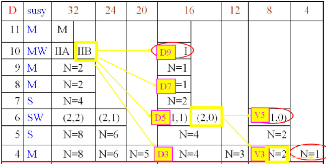
Figure 1: The IIB supergravities have solutions denoted as D9,D7,D5,D3. The (2,0) theory has solutions V5,V3 and $N=2$ supergravity has a $N=1$ solution. The red circles indicate the basic super-Maxwell theories that we started from in the bottom-up approach and are obtained as maximal $p$ theories.

The supergravities with each a doublet of local symmetries from which one starts are indicated as open yellow boxes. The branes type DBI actions are the D9,D7,D5,D3 when we start from $D=10$, and are indicated as V5 and V3 when we start from $D=6$. The V stands for vector branes as explained in the talk of Eric Bergshoeff. This thus shows that we can construct deformed super-Maxwell theories for various dimensions and supersymmetry extensions, including ${\cal N}=4$, ${\cal N}=2$ and ${\cal N}=1$ in 4 dimensions.

0.5.3 $D=4$, ${\cal N}=4$ gauge multiplet

Let us in particular consider the D3 case, i.e. the $D=4$, ${\cal N}=4$ theory that we discussed in previous sections. The full action of the deformed theory is

$$S=-\frac{1}{\alpha^{2}}\int{\rm d}^{4}x\,\left\{\sqrt{-\det(G_{\mu\nu}+\alpha{\cal F}_{\mu\nu})}-1\right\}\,,\qquad\mu=0,1,2,3\,,$$ (40)

with

$$G_{\mu\nu} = \eta_{mn}\Pi_{\mu}^{m}\Pi_{\nu}^{n}=\eta_{m^{\prime}n^{\prime}}\Pi_{\mu}^{m^{\prime}}\Pi_{\nu}^{n^{\prime}}+\delta_{IJ}\Pi_{\mu}^{I}\Pi_{\nu}^{J}\,,\quad m^{\prime}=0,1,2,3\,,$$

$$\Pi_{\mu}^{m^{\prime}} = \delta^{m^{\prime}}_{\mu}+{\textstyle\frac{1}{2}}\alpha^{2}\bar{\lambda}\Gamma^{m^{\prime}}\partial_{\mu}\lambda\ ,\qquad\Pi_{\mu}^{I}=\partial_{\mu}\phi^{I}+{\textstyle\frac{1}{2}}\alpha^{2}\bar{\lambda}\Gamma^{I}\partial_{\mu}\lambda\,,\quad I=1,...,6\,,$$

$${\cal F}_{\mu\nu} \equiv F_{\mu\nu}+\alpha\bar{\lambda}\Gamma_{[\mu}\partial_{\nu]}\lambda+\alpha\bar{\lambda}\Gamma_{I}\partial_{[\mu}\lambda\partial_{\nu]}\phi^{I}\,.$$ (41)

There are 16 $\epsilon$ and 16 $\zeta$ symmetries, and the remainders of the rigid Poincaré transformations in $D=10$ lead to shift symmetries for the 6 scalars $\phi^{I}$. We can compare this with the usual formulation of the ${\cal N}=4$, $D=4$ super-Maxwell theory:

$$S_{\rm Maxw}=\int{\rm d}^{4}x\Big{(}-{\textstyle\frac{1}{4}}F_{\mu\nu}F^{\mu\nu}-\bar{\psi}_{i}\not{\partial}\psi^{i}-{\textstyle\frac{1}{8}}\partial_{\mu}\varphi_{ij}\partial^{\mu}\varphi^{ij}\Big{)}\,.$$ (42)

$F_{\mu\nu}$ is the field strength of the vector field, the $\psi_{i}$ are 4 Majorana spinors, written as Weyl spinors using the notations $\psi^{i}={\textstyle\frac{1}{2}}(1+\gamma_{*})\psi^{i}$ and $\psi_{i}={\textstyle\frac{1}{2}}(1-\gamma_{*})\psi_{i}$. The 6 scalar fields are here represented as antisymmetric tensors $\varphi_{ij}$, with

$$\varphi^{ij}\equiv(\varphi_{ij})^{*}=-{\textstyle\frac{1}{2}}\varepsilon^{ijk\ell}\varphi_{k\ell}\,.$$ (43)

One can find (42) and the transformation laws as the $\alpha=0$ part of (40) and (36), by making some identifications. The scalars $\phi^{I}$ representing the 6 remaining coordinates in $D=10$ according to (33) are divided in two triplets $\phi_{a}$ and $\phi_{a+3}$ and we identify

$$\alpha\varphi_{ij}=\phi_{a}\beta_{ij}^{a}-{\rm i}\phi_{a+3}\alpha^{a}_{ij}\,,\qquad a=1,2,3\,,$$ (44)

where $\alpha^{a}_{ij}$ and $\beta_{ij}^{a}$ are the Gliozzi–Scherk–Olive $4\times 4$ matrices Brink:1976bc ; Gliozzi:1976qd . These are also used to identify the $D=10$ Majorana-Weyl spinor $\lambda$ introduced in (33), with the 4 Majorana spinors $\psi^{i}$. This is done with the $D=10$ gamma matrix representation

$$\Gamma^{\mu} = \gamma^{\mu}\otimes\mathord{\!\leavevmode\hbox{ \begin{picture}(0.6,0.7)\put(0.0,0.0){\line(1,0){0.5}} \put(0.15,0.0){\line(0,1){0.7}} \put(0.35,0.0){\line(0,1){0.8}} \put(0.3,0.8){\rule{0.5pt}{0.5pt}}\put(0.26,0.78){\rule{0.5pt}{0.5pt}}\put(0.22,0.76){\rule{0.5pt}{0.5pt}}\put(0.18,0.74){\rule{0.5pt}{0.5pt}}\put(0.14,0.72){\rule{0.5pt}{0.5pt}}\put(0.1,0.7){\rule{0.5pt}{0.5pt}}\put(0.06,0.68){\rule{0.5pt}{0.5pt}}\put(0.02,0.66){\rule{0.5pt}{0.5pt}}\put(-0.02,0.64){\rule{0.5pt}{0.5pt}}\put(-0.06,0.62){\rule{0.5pt}{0.5pt}}\put(-0.1,0.6){\rule{0.5pt}{0.5pt}}\put(-0.14,0.58){\rule{0.5pt}{0.5pt}} \end{picture}}}_{8}\,,\quad\Gamma^{a}=\gamma_{*}\otimes\pmatrix{0&\beta^{a}\cr-\beta^{a}&0}\,,\quad\Gamma^{a+3}=\gamma_{*}\otimes\pmatrix{0&{\rm i}\alpha^{a}\cr{\rm i}\alpha^{a}&0}\,,$$

$$C_{10} = C_{4}\otimes\pmatrix{0&\mathord{\!\leavevmode\hbox{ \begin{picture}(0.6,0.7)\put(0.0,0.0){\line(1,0){0.5}} \put(0.15,0.0){\line(0,1){0.7}} \put(0.35,0.0){\line(0,1){0.8}} \put(0.3,0.8){\rule{0.5pt}{0.5pt}}\put(0.26,0.78){\rule{0.5pt}{0.5pt}}\put(0.22,0.76){\rule{0.5pt}{0.5pt}}\put(0.18,0.74){\rule{0.5pt}{0.5pt}}\put(0.14,0.72){\rule{0.5pt}{0.5pt}}\put(0.1,0.7){\rule{0.5pt}{0.5pt}}\put(0.06,0.68){\rule{0.5pt}{0.5pt}}\put(0.02,0.66){\rule{0.5pt}{0.5pt}}\put(-0.02,0.64){\rule{0.5pt}{0.5pt}}\put(-0.06,0.62){\rule{0.5pt}{0.5pt}}\put(-0.1,0.6){\rule{0.5pt}{0.5pt}}\put(-0.14,0.58){\rule{0.5pt}{0.5pt}} \end{picture}}}_{4}\cr\mathord{\!\leavevmode\hbox{ \begin{picture}(0.6,0.7)\put(0.0,0.0){\line(1,0){0.5}} \put(0.15,0.0){\line(0,1){0.7}} \put(0.35,0.0){\line(0,1){0.8}} \put(0.3,0.8){\rule{0.5pt}{0.5pt}}\put(0.26,0.78){\rule{0.5pt}{0.5pt}}\put(0.22,0.76){\rule{0.5pt}{0.5pt}}\put(0.18,0.74){\rule{0.5pt}{0.5pt}}\put(0.14,0.72){\rule{0.5pt}{0.5pt}}\put(0.1,0.7){\rule{0.5pt}{0.5pt}}\put(0.06,0.68){\rule{0.5pt}{0.5pt}}\put(0.02,0.66){\rule{0.5pt}{0.5pt}}\put(-0.02,0.64){\rule{0.5pt}{0.5pt}}\put(-0.06,0.62){\rule{0.5pt}{0.5pt}}\put(-0.1,0.6){\rule{0.5pt}{0.5pt}}\put(-0.14,0.58){\rule{0.5pt}{0.5pt}} \end{picture}}}_{4}&0}\,,\qquad\Gamma_{*}=\gamma_{*}\otimes\pmatrix{\mathord{\!\leavevmode\hbox{ \begin{picture}(0.6,0.7)\put(0.0,0.0){\line(1,0){0.5}} \put(0.15,0.0){\line(0,1){0.7}} \put(0.35,0.0){\line(0,1){0.8}} \put(0.3,0.8){\rule{0.5pt}{0.5pt}}\put(0.26,0.78){\rule{0.5pt}{0.5pt}}\put(0.22,0.76){\rule{0.5pt}{0.5pt}}\put(0.18,0.74){\rule{0.5pt}{0.5pt}}\put(0.14,0.72){\rule{0.5pt}{0.5pt}}\put(0.1,0.7){\rule{0.5pt}{0.5pt}}\put(0.06,0.68){\rule{0.5pt}{0.5pt}}\put(0.02,0.66){\rule{0.5pt}{0.5pt}}\put(-0.02,0.64){\rule{0.5pt}{0.5pt}}\put(-0.06,0.62){\rule{0.5pt}{0.5pt}}\put(-0.1,0.6){\rule{0.5pt}{0.5pt}}\put(-0.14,0.58){\rule{0.5pt}{0.5pt}} \end{picture}}}_{4}&0\cr 0&-\mathord{\!\leavevmode\hbox{ \begin{picture}(0.6,0.7)\put(0.0,0.0){\line(1,0){0.5}} \put(0.15,0.0){\line(0,1){0.7}} \put(0.35,0.0){\line(0,1){0.8}} \put(0.3,0.8){\rule{0.5pt}{0.5pt}}\put(0.26,0.78){\rule{0.5pt}{0.5pt}}\put(0.22,0.76){\rule{0.5pt}{0.5pt}}\put(0.18,0.74){\rule{0.5pt}{0.5pt}}\put(0.14,0.72){\rule{0.5pt}{0.5pt}}\put(0.1,0.7){\rule{0.5pt}{0.5pt}}\put(0.06,0.68){\rule{0.5pt}{0.5pt}}\put(0.02,0.66){\rule{0.5pt}{0.5pt}}\put(-0.02,0.64){\rule{0.5pt}{0.5pt}}\put(-0.06,0.62){\rule{0.5pt}{0.5pt}}\put(-0.1,0.6){\rule{0.5pt}{0.5pt}}\put(-0.14,0.58){\rule{0.5pt}{0.5pt}} \end{picture}}}_{4}}\,,$$ (45)

where $C_{10}$ and $C_{4}$ are the charge conjugation matrices (for notation, see Freedman:2012zz ) in 10 and 4 dimensions, and $\gamma^{\mu}$ are the $D=4$ gamma matrices. In this basis, $\lambda$ is decomposed as

$$\lambda=\pmatrix{\psi^{i}\cr\psi_{i}}\,.$$ (46)

With these identifications, the $\alpha=0$ part of (40) agrees with (42). Since the action (40) is invariant to all orders in $\alpha$ under the $16+16$ supersymmetries, it gives the fully consistent deformation of the ${\cal N}=4$, $D=4$ gauge multiplet. It has both type of supersymmetries: ordinary SUSY and VA-type supersymmetry. It can be written in the usual 4-dimensional notations using the translations (44) and (46), but the $D=10$ formulation is much simpler.

0.5.4 Worldvolume theory in AdS background

In order to make progress for ${\cal N}=4$, $D=4$ supergravity, we would need the deformed gauge multiplet with the superconformal symmetries. The extra VA symmetries are not of the type of $S$-supersymmetry. Inspiration may come from old work Claus:1997cq ; Claus:1998mw ; Claus:1998ts where the worldvolume theories of branes were considered in an AdS background, leading to a superconformal theory on the brane. The AdS backgrounds exist only in particular dimensions and extensions, corresponding to the fact that the superconformal theories also only exist for particular cases as explained at the end of Sect. 0.3, see Table 7. These actions on the brane are of the form

$$S_{cl} = S_{\rm DBI}+S_{\rm WZ}\,,$$

$$S_{\rm DBI} = -\int{\rm d}^{p+1}\sigma\sqrt{-\det\left(g^{\rm ind}_{\mu\nu}+F_{\mu\nu}\right)}\,,$$

$$g^{\rm ind}_{\mu\nu} = \partial_{\mu}X^{M}\partial_{\nu}X^{N}G_{MN}\,,$$ (47)

where $G_{MN}$ denotes the AdS $\times$ sphere metric that is a solution of the embedding theory. The theory has then rigid symmetries inherited from the solution. These are the AdS isometries and the isometries of the sphere and the corresponding supersymmetries. The brane theory has as in Sect. 0.5.2 the worldvolume general coordinate transformations and kappa symmetries as local symmetries. After gauge fixing these, the remaining (global) symmetries appear as conformal symmetries on the brane. The fermionic ones are then $\epsilon$ ordinary supersymmetry and $\eta$ special supersymmetry. Hence this is very similar to the appearance of ordinary and VA type supersymmetries in our new work Bergshoeff:2013pia . This gives us a hope to obtain an all-order deformation of gauge multiplet theories with superconformal symmetries in the cases where the superalgebras exist, which includes the D3 brane with ${\cal N}=4$, $D=4$ supersymmetry.

0.6 Conclusions

Superconformal symmetry has been used as a tool for constructing classical actions of supergravity. Also higher-derivative terms can be constructed with superconformal tensor calculus Hanaki:2006pj ; deWit:2010za ; Bergshoeff:2011xn ; Bergshoeff:2012ax ; Ozkan:2013uk . Quantum calculations show that there are unknown relevant properties of supergravity theories. We have investigated the possibility that (broken) superconformal symmetry be such an extra quantum symmetry Ferrara:2012ui . The non-existence of (broken) superconformal-invariant counterterms and anomalies for ${\cal N}=4$, $D=4$ supergravity could in that case explain miraculous vanishing results. However, we do not have a systematic knowledge of which higher-derivative supergravity actions can be invariant under supersymmetry at all orders in derivatives.

In order to get more insight, we have been looking to gauge multiplets in global supersymmetry Bergshoeff:2013pia . We first considered a perturbative approach, i.e. constructing actions and transformation laws order by order in a dimensionful parameter $\alpha$, which can be related to the string coupling constant. Starting from D$p$ brane actions in $D=10$ we can construct DBI-type actions that have ordinary supersymmetry plus VA-type supersymmetry with 16+16 components. They are related to IIB supergravity, and thus exist for $p=9,7,5,3,...$, leading to global supersymmetry actions for gauge multiplets in $p+1$ dimensions. For $p=3$ this is the deformation of ${\cal N}=4$, $D=4$ with higher order derivatives. One can also start from the iib theory in $D=6$. Also in that case DBI-VA actions (related to objects called vector branes or ‘V-branes’ Bergshoeff:2012jb ) with 8+8 supersymmetries. This leads e.g. to the deformation of $D=4$, ${\cal N}=2$ vector multiplets. We hope that insight in these new constructions can lead also to supergravity actions using the superconformal methods.

0.7 Acknowledgements

Most results in this paper are obtained in collaboration with E. Bergshoeff, F. Coomans, R. Kallosh, S. Ferrara and C. S. Shahbazi, and part of the talk has been prepared in collaboration with R. Kallosh. We thank S. Bellucci and other organizers of this topical meeting, which was very stimulating.

This work was supported in part by the FWO - Vlaanderen, Project No. G.0651.11, and in part by the Interuniversity Attraction Poles Programme initiated by the Belgian Science Policy (P7/37).

References

- (1) D. Z. Freedman and A. Van Proeyen, Supergravity. Cambridge University Press, 2012.
- (2) J. Strathdee, Extended Poincaré supersymmetry, Int. J. Mod. Phys. A2 (1987) 273
- (3) F. Cordaro, P. Frè, L. Gualtieri, P. Termonia and M. Trigiante, gaugings revisited: An exhaustive classification, Nucl. Phys. B532 (1998) 245–279, arXiv:hep-th/9804056
- (4) H. Nicolai and H. Samtleben, Compact and noncompact gauged maximal supergravities in three dimensions, JHEP 04 (2001) 022, hep-th/0103032
- (5) B. de Wit, H. Samtleben and M. Trigiante, Magnetic charges in local field theory, JHEP 09 (2005) 016, hep-th/0507289
- (6) E. Bergshoeff, M. de Roo and B. de Wit, Extended conformal supergravity, Nucl. Phys. B182 (1981) 173
- (7) M. de Roo, Matter coupling in supergravity, Nucl.Phys. B255 (1985) 515
- (8) W. Nahm, Supersymmetries and their representations, Nucl. Phys. B135 (1978) 149
- (9) J. W. van Holten and A. Van Proeyen, supersymmetry algebras in mod. 8, J. Phys. A15 (1982) 3763
- (10) R. D’Auria, S. Ferrara, M. A. Lledó and V. S. Varadarajan, Spinor algebras, J. Geom. Phys. 40 (2001) 101–128, hep-th/0010124
- (11) E. Bergshoeff, M. de Roo and B. de Wit, Conformal supergravity in ten dimensions, Nucl. Phys. B217 (1983) 489
- (12) Z. Bern, J. Carrasco, L. J. Dixon, H. Johansson, D. Kosower et al., Three-loop superfiniteness of supergravity, Phys.Rev.Lett. 98 (2007) 161303, arXiv:hep-th/0702112 [hep-th]
- (13) Z. Bern, J. Carrasco, L. J. Dixon, H. Johansson and R. Roiban, The ultraviolet behavior of supergravity at four loops, Phys.Rev.Lett. 103 (2009) 081301, arXiv:0905.2326 [hep-th]
- (14) Z. Bern, S. Davies, T. Dennen and Y.-t. Huang, Absence of three-loop four-point divergences in supergravity, Phys.Rev.Lett. 108 (2012) 201301, arXiv:1202.3423 [hep-th]
- (15) S. Cecotti and S. Ferrara, Supersymmetric Born-Infeld Lagrangians, Phys.Lett. B187 (1987) 335
- (16) B. de Wit, S. Katmadas and M. van Zalk, New supersymmetric higher-derivative couplings: Full superspace does not count!, JHEP 1101 (2011) 007, arXiv:1010.2150 [hep-th]
- (17) W. Chemissany, S. Ferrara, R. Kallosh and C. Shahbazi, supergravity counterterms, off and on shell, JHEP 12 (2012) 089, arXiv:1208.4801 [hep-th]
- (18) S. Ferrara, R. Kallosh and A. Van Proeyen, Conjecture on hidden superconformal symmetry of Supergravity, Phys.Rev. D87 (2013) 025004, arXiv:1209.0418 [hep-th]
- (19) E. Bergshoeff, F. Coomans, R. Kallosh, C. Shahbazi and A. Van Proeyen, Dirac-Born-Infeld-Volkov-Akulov and Deformation of Supersymmetry, arXiv:1303.5662 [hep-th]
- (20) E. Bergshoeff, M. Rakowski and E. Sezgin, Higher derivative super-Yang-Mills theories, Phys.Lett. B185 (1987) 371
- (21) M. Aganagic, C. Popescu and J. H. Schwarz, Gauge invariant and gauge fixed D-brane actions, Nucl.Phys. B495 (1997) 99–126, arXiv:hep-th/9612080 [hep-th]
- (22) E. A. Bergshoeff and F. Riccioni, Heterotic wrapping rules, JHEP 1301 (2013) 005, arXiv:1210.1422 [hep-th]
- (23) L. Brink, J. H. Schwarz and J. Scherk, Supersymmetric Yang-Mills theories, Nucl.Phys. B121 (1977) 77
- (24) F. Gliozzi, J. Scherk and D. I. Olive, Supersymmetry, supergravity theories and the dual spinor model, Nucl.Phys. B122 (1977) 253–290
- (25) P. Claus, R. Kallosh and A. Van Proeyen, M 5-brane and superconformal (0,2) tensor multiplet in 6 dimensions, Nucl. Phys. B518 (1998) 117–150, hep-th/9711161
- (26) P. Claus, R. Kallosh, J. Kumar, P. K. Townsend and A. Van Proeyen, Conformal theory of M2, D3, M5 and D1+D5 branes, JHEP 06 (1998) 004, hep-th/9801206
- (27) P. Claus, M. Derix, R. Kallosh, J. Kumar, P. K. Townsend and A. Van Proeyen, Black holes and superconformal mechanics, Phys. Rev. Lett. 81 (1998) 4553–4556, hep-th/9804177
- (28) K. Hanaki, K. Ohashi and Y. Tachikawa, Supersymmetric completion of an term in five-dimensional supergravity, Prog.Theor.Phys. 117 (2007) 533, arXiv:hep-th/0611329 [hep-th]
- (29) E. A. Bergshoeff, J. Rosseel and E. Sezgin, Off-shell , Riemann squared supergravity, Class.Quant.Grav. 28 (2011) 225016, arXiv:1107.2825 [hep-th]
- (30) E. Bergshoeff, F. Coomans, E. Sezgin and A. Van Proeyen, Higher derivative extension of 6 chiral gauged supergravity, JHEP 1207 (2012) 011, arXiv:1203.2975 [hep-th]
- (31) M. Ozkan and Y. Pang, Supersymmetric completion of Gauss-Bonnet combination in five dimensions, JHEP 1303 (2013) 158, arXiv:1301.6622 [hep-th]