Ground state of the asymmetric Rabi model in the ultrastrong coupling regime

Abstract

We study the ground states of the single- and two-qubit asymmetric Rabi models, in which the qubit-oscillator coupling strengths for the counterrotating-wave and corotating-wave interactions are unequal. We take the transformation method to obtain the approximately analytical ground states for both models and numerically verify its validity for a wide range of parameters under the near-resonance condition. We find that the ground-state energy in either the single- or two-qubit asymmetric Rabi model has an approximately quadratic dependence on the coupling strengths stemming from different contributions of the counterrotating-wave and corotating-wave interactions. For both models, we show that the ground-state energy is mainly contributed by the counterrotating-wave interaction. Interestingly, for the two-qubit asymmetric Rabi model, we find that, with the increase of the coupling strength in the counterrotating-wave or corotating-wave interaction, the two-qubit entanglement first reaches its maximum then drops to zero. Furthermore, the maximum of the two-qubit entanglement in the two-qubit asymmetric Rabi model can be much larger than that in the two-qubit symmetric Rabi model.

I Introduction

The Rabi model PR-49-324-1936 , describing the interaction between a two-level system and a quantized harmonic oscillator, is a fundamental model in quantum optics. For the cavity quantum electrodynamics (QED) experiments, the qubit-oscillator coupling strength of the Rabi model is far smaller than the oscillator’s frequency and the corotating-wave approximation (RWA) works well, bringing in the ubiquitous Jaynes-Cummins model IEEE-51-89-1963 ; JMO-40-1195-1993 ; PRL-87-037902-2001 ; PRA-71-013817-2005 . With recent experiment progresses in Rabi models PT-58-42-2005 ; Science-326-108-2009 ; PR-492-1-2010 ; RPP-74-104401-2011 ; Nature-474-589-2011 ; RMP-84-1-2012 ; RMP-85-623-2013 ; arxiv1308-6253-2014 in the ultrastrong coupling regime PRB-78-180502-2008 ; PRB-79-201303-2009 ; Nature-458-178-2009 ; Nature-6-772-2010 ; PRL-105-237001-2010 ; PRL-105-196402-2010 ; PRL-106-196405-2011 ; Science-335-1323-2012 ; PRL-108-163601-2012 ; PRB-86-045408-2012 ; NatureCommun-4-1420-2013 , in which the qubit-oscillator coupling strength becomes a considerable fraction of the oscillator’s or qubit’s frequency, the RWA breaks down but relatively complex quantum dynamics arises, bringing about many fascinating quantum phenomena NJP-13-073002-2011 ; PRL-109-193602-2012 ; PRA-81-042311-2010 ; PRA-87-013826-2013 ; PRA-59-4589-1999 ; PRA-62-033807-2000 ; PRB-72-195410-2005 ; PRA-74-033811-2006 ; PRA-77-053808-2008 ; PRA-82-022119-2010 ; PRL-107-190402-2011 ; PRL-108-180401-2012 ; PLA-376-349-2012 .

Explicitly analytic solution to the Rabi model beyond the RWA is hard to obtain due to the non-integrability in its infinite-dimensional Hilbert space. Since it is difficult to capture the physics through numerical solution JPA-29-4035-1996 ; EPL-96-14003-2011 , various approximately analytical methods for obtaining the ground states of the symmetric Rabi models (SRM) have been tried RPB-40-11326-1989 ; PRB-42-6704-1990 ; PRL-99-173601-2007 ; EPL-86-54003-2009 ; PRA-80-033846-2009 ; PRL-105-263603-2010 ; PRA-82-025802-2010 ; EPJD-66-1-2012 ; PRA-86-015803-2012 ; PRA-85-043815-2012 ; PRA-86-023822-2012 ; EPJB-38-559-2004 ; PRB-75-054302-2007 ; EPJD-59-473-2010 ; arXiv-1303-3367v2-2013 ; arXiv-1305-1226-2013 ; PRA-87-022124-2013 ; PRA-86-014303-2012 ; arXiv-1305-6782-2013 . Especially, Braak PRL-107-100401-2011 used the method based on the $Z_{2}$ symmetry to analytically determine the spectrum of the single-qubit Rabi model, which was dependent on the composite transcendental function defined through its power series but failed to derive the concrete form of the system’s ground state. In Ref. PRA-81-042311-2010 , Ashhab et al. applied the method of adiabatic approximation to treat two extreme situations to obtain the eigenstates and eigenenergies in the single-qubit SRM, i.e., the situation with a high-frequency oscillator or a high-frequency qubit. Ashhab PRA-87-013826-2013 used different order parameters to identify the phase regions of the single-qubit SRM and found that the phase-transition-like behavior appeared when the oscillator’s frequency was much lower than the qubit’s frequency. Lee and Law arXiv-1303-3367v2-2013 used the transformation method to seek the approximately analytical ground state of the two-qubit SRM in the near-resonance regime, and found that the two-qubit entanglement drops as the coupling strength further increased after it reached its maximum.

Previous studies consider the ground state of the SRM, i.e., the qubit-oscillator coupling strengths of the counterrotating-wave and corotating-wave interactions are equal. In this paper, we study the asymmetic Rabi models (ASRM), i.e., the coupling strengths for the counterrotating-wave and corotating-wave interactions are unequal, which helps to gain deep insight into the fundamentally physical property of such models. Different from Refs. PRA-81-042311-2010 ; PRA-87-013826-2013 , we here use the transformation method to obtain the ground state of the single-qubit ASRM under the near-resonance situation, where the oscillator’s frequency approximates the qubit’s frequency. Differ further from Ref. arXiv-1303-3367v2-2013 , our investigation for the two-qubit ASRM intuitively identifies the collective contribution to its ground-state entanglement caused by the corotating-wave and counterrotating-wave interactions.

We investigate the single- and two-qubit ASRMs and show that their approximately analytical ground states agree well with the exactly numerical solutions for a wide range of parameters under the near-resonance situation, and the ground-state energy has an approximately quadratic dependence on the coupling strengths stemming from contributions of the counterrotating-wave and corotating-wave interactions. Besides, we show that the ground-state energy is mainly contributed by the counterrotating-wave interaction in both models. For the two-qubit ASRM, we obtain the approximately analytical negativity. Interestingly, for the two-qubit ASRM, we find that, with the increase of the coupling strength in the counterrotating-wave or corotating-wave interaction, the two-qubit entanglement first reaches its maximum then drops to zero.

The advantages of our result are the collective contributions to the ground state of the ASRM caused by the corotating-wave interaction and counterrotating-wave interaction can be determined approximately, and the contribution of the counterrotating-wave interaction on the ground state energy is larger than that of the corotating-wave interaction. We find that the maximal two-qubit entanglement of the ASRM is larger than that in the case of SRM. However, the transformation method here is applicable to the ASRM only under the near-resonant regime, where the oscillator’s frequency approximates the qubit’s frequency. When the corotating-wave and counterrotating-wave coupling constants are large enough in the ASRM, the result obtained by the transformation method has a big error compared with that obtained by the exactly numerical method. Such an investigation can also be generalized to the complex cases of three- and more-qubit ASRM. Note that the ASRM can be realized by using two unbalanced Raman channels between two atomic ground states induced by a cavity mode and two classical fields in theory PRA-75-013804-2007 .

II The single-qubit ASRM

II.1 Transformed ground state

The Hamiltonian of the single-qubit ASRM is PRA-8-1440-1973 : (assume $\hbar=1$ for simplicity hereafter)

$$H_{1} = \frac{1}{2}w_{a}\sigma_{z}+w_{b}b^{\dagger}b$$ (2)

$$+\frac{\lambda_{1}}{2}(b^{\dagger}\sigma_{-}+b\sigma_{+})+\frac{\lambda_{2}}{2}(b^{\dagger}\sigma_{+}+b\sigma_{-}),$$

where $w_{a}$ is the qubit’s frequency. $\sigma_{z}$ and $\sigma_{\pm}$ are the Pauli matrices, describing the qubit’s energy operator and the spin-flip operators, respectively. We assume that $|\downarrow\rangle_{A}$ and $|\uparrow\rangle_{A}$ are the eigenstates of $\sigma_{z}$, i.e., $\sigma_{z}$ $|\downarrow\rangle_{A}$ $=$ $-|\downarrow\rangle_{A}$ and $\sigma_{z}$ $|\uparrow\rangle_{A}$ $=$ $|\uparrow\rangle_{A}$. $b^{\dagger}$ ($b$) is the creation (annihilation) operator of the harmonic oscillator with the frequency $w_{b}$. The qubit-oscillator coupling strengths of the corotating-wave interaction $(b^{\dagger}\sigma_{-}+b\sigma_{+})$ and the counterrotating-wave interaction $(b^{\dagger}\sigma_{+}+b\sigma_{-})$ are denoted by $\lambda_{1}$ and $\lambda_{2}$, respectively. However, when $\lambda_{1}$ $\neq$ $\lambda_{2}$ (here $\lambda_{1}$, $\lambda_{2}$, $w_{a}$ $\neq 0$), to our knowledge, there is still no analytical solution to the ground state of the single-qubit ASRM.

Our task in this paper is to determine the ground-state energy $E_{g}$ and the ground-state vector $|\phi_{g}\rangle$ for the single- (Section II) or two-qubit (Section III) ASRM, where $H_{1}|\phi_{g}\rangle$ $=$ $E_{g}|\phi_{g}\rangle$. In this paper, the subscripts $A$ and $F$ denote the vectors of the atomic state and field state, respectively.

To deal with the counterrotating-wave terms in Eq. (2), we apply a unitary transformation to the Hamiltonian $H_{1}$ EPJD-59-473-2010 ; PRB-75-054302-2007 ; PRA-82-022119-2010 :

$$H_{1}^{{}^{\prime}} = e^{S_{1}}H_{1}e^{-S_{1}},$$ (3)

with

$$S_{1}=\xi_{1}(b^{\dagger}-b)\sigma_{x},$$ (4)

where $\xi_{1}$ is a variable to be determined later. Then the transformed Hamiltonian $H_{1}^{{}^{\prime}}$ can be decomposed into three parts:

$$H_{1}^{{}^{\prime}} = H_{1}^{a}+H_{1}^{b}+H_{1}^{c},$$ (5)

with

$$H_{1}^{a} = \frac{1}{2}\big{[}w_{a}\eta_{1}-(\lambda_{1}-\lambda_{2})\xi_{1}\eta_{1}\big{]}\sigma_{z}$$ (10)

$$+\big{[}w_{b}-(\lambda_{1}-\lambda_{2})\xi_{1}\eta_{1}\sigma_{z}\big{]}b^{\dagger}b$$

$$+w_{b}\xi_{1}^{2}-\frac{1}{2}(\lambda_{1}+\lambda_{2})\xi_{1},$$

$$H_{1}^{b} = \big{[}\frac{1}{4}(\lambda_{1}+\lambda_{2})-w_{b}\xi_{1}\big{]}(b^{\dagger}+b)\sigma_{x}$$ (13)

$$-i\big{[}\frac{1}{4}(\lambda_{1}-\lambda_{2})\eta_{1}+w_{a}\xi_{1}\eta_{1}\big{]}(b^{\dagger}-b)\sigma_{y},$$

$$H_{1}^{c} = \frac{1}{2}w_{a}\sigma_{z}\bigg{\{}\cosh\big{[}2\xi_{1}(b^{\dagger}-b)\big{]}-\eta_{1}\bigg{\}}$$ (18)

$$-\frac{i}{2}w_{a}\sigma_{y}\bigg{\{}\sinh\big{[}2\xi_{1}(b^{\dagger}-b)\big{]}-2\xi_{1}\eta_{1}(b^{\dagger}-b)\bigg{\}}$$

$$-\frac{i}{4}(\lambda_{1}-\lambda_{2})(b^{\dagger}-b)\sigma_{y}\bigg{\{}\cosh\big{[}2\xi_{1}(b^{\dagger}-b)\big{]}$$

$$-\eta_{1}\bigg{\}}+\frac{1}{4}(\lambda_{1}-\lambda_{2})(b^{\dagger}-b)\sigma_{z}\bigg{\{}\sinh\big{[}2\xi_{1}(b^{\dagger}$$

$$-b)\big{]}-2\xi_{1}\eta_{1}(b^{\dagger}-b)\bigg{\}}+O(b^{\dagger 2},b^{2}),$$

where $\eta_{1}$$=_{F}$$\langle 0|\cosh[2\xi_{1}(b^{\dagger}-b)]|0\rangle_{F}$ $=$ $e^{-2\xi_{1}^{2}}$ and $O(b^{\dagger 2},b^{2})=\frac{1}{2}(\lambda_{1}-\lambda_{2})\xi_{1}\eta_{1}(b^{\dagger 2}+b^{2})\sigma_{z}$. The terms $\cosh[2\xi_{1}(b^{\dagger}-b)]$ and $\sinh[2\xi_{1}(b^{\dagger}-b)]$ in $H_{1}^{c}$ have the dominating expansions EPJD-59-473-2010 :

$$\cosh[2\xi_{1}(b^{\dagger}-b)] \simeq \eta_{1}+O(\xi_{1}^{2}),$$ (19)

$$\sinh[2\xi_{1}(b^{\dagger}-b)] \simeq 2\xi_{1}\eta_{1}(b^{\dagger}-b)+O(\xi_{1}^{3}),$$ (20)

where $O(b^{\dagger 2},b^{2})$, $O(\xi_{1}^{2})$ and $O(\xi_{1}^{3})$ are higher-order terms of $b^{\dagger}$ and $b$, which represent the double- and three-photon transition processes and can be neglected as an approximation when $\xi_{1}$ and $|\lambda_{1}\pm\lambda_{2}|$ are much smaller than the frequency sum $w_{a}+w_{b}$ where $w_{a}\approx w_{b}$. Thus, $H_{1}^{{}^{\prime}}\simeq H_{1}^{a}+H_{1}^{b}$.

When the parameter $\xi_{1}$ is chosen such that it satisfies the condition:

$$e^{2\xi_{1}^{2}}\big{[}(\lambda_{1}+\lambda_{2})-4w_{b}\xi_{1}\big{]}=(\lambda_{1}-\lambda_{2})+4w_{a}\xi_{1},$$ (21)

the qubit and the oscillator are coupled in the following form:

$$H_{1}^{b} = \frac{1}{2}\big{[}(\lambda_{1}+\lambda_{2})-4w_{b}\xi_{1}\big{]}\times\big{(}b^{\dagger}\sigma_{-}+b\sigma_{+}\big{)}.$$ (22)

Note that $H_{1}^{b}$ in Eq. (22) contains no counterrotating-wave interactions in which the qubit excitation (deexcitation) is accompanied by the emission (absorption) of a photon. Therefore, the transformed Hamiltonian $H_{1}^{{}^{\prime}}$ is exactly solvable when we eliminate the counterrotating-wave terms by choosing $\xi_{1}$ to satisfy Eq. (21) and by neglecting higher-order transition processes which are presented by terms $O(b^{\dagger 2},b^{2})$, $O(\xi_{1}^{2})$ and $O(\xi_{1}^{3})$.

It is easy to show that the eigenvector $|\downarrow\rangle_{A}|0\rangle_{F}$ is the ground-state vector of the transformed Hamiltonian $H_{1}^{{}^{\prime}}$, with $|0\rangle_{F}$ being the vacuum state of the harmonic oscillator, and the corresponding eigenenergy $E_{g1}$ is:

$$E_{g1}=\xi_{1}^{2}w_{b}-\frac{1}{2}(\lambda_{1}+\lambda_{2})\xi_{1}-\frac{1}{2}\eta_{1}[w_{a}-\xi_{1}(\lambda_{1}-\lambda_{2})].$$ (23)

We see that when $\lambda_{1}=\lambda_{2}$, $E_{g1}$ reduces to the transformed ground-state energy derived in Ref. EPJD-59-473-2010 . Therefore, the ground state of the original Hamiltonian (2) can be approximately constructed:

$$|\phi_{g1}\rangle = e^{-S_{1}}|\downarrow\rangle_{A}|0\rangle_{F}$$ (25)

$$= \frac{1}{\sqrt{2}}(|\psi_{A}^{+}\rangle|-\xi_{1}\rangle_{F}-|\psi_{A}^{-}\rangle|\xi_{1}\rangle_{F}),$$ (26)

with $|\xi_{1}\rangle_{F}$ and $|-\xi_{1}\rangle_{F}$ being the coherent states of the oscillator with the amplitudes $\xi_{1}$ and $-\xi_{1}$. $|\psi_{A}^{+}\rangle=(|\uparrow\rangle_{A}+|\downarrow\rangle_{A})/\sqrt{2}$ and $|\psi_{A}^{-}\rangle=(|\uparrow\rangle_{A}-|\downarrow\rangle_{A})/\sqrt{2}$ are the eigenstates of $\sigma_{x}$.

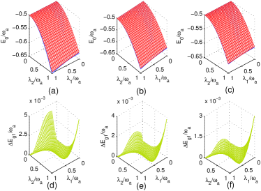
Figure 1: (Color online) The ground-state energy for the single-qubit ASRM obtained by the transformation method $E_{0}=E_{g1}$ (red grid) and by the numerical solution $E_{0}=E_{g}$ (blue grid) versus the coupling strengths $\lambda_{1}$ and $\lambda_{2}$: (a) $w_{b}=0.8w_{a}$; (b) $w_{b}=w_{a}$; (c) $w_{b}=1.2w_{a}$. The energy deviation $\Delta E_{g1}=E_{g1}-E_{g}$ versus $\lambda_{1}$ and $\lambda_{2}$: (d) $w_{b}=0.8w_{a}$; (e) $w_{b}=w_{a}$; (f) $w_{b}=1.2w_{a}$.

The value of $\xi_{1}$ is obtained by numerically solving the nonlinear equation (21). $\xi_{1}$ has an approximately linear dependence on the counterrotating-wave coupling strength by neglecting high-order terms of the field mode as:

$$\xi_{1} \simeq \frac{\lambda_{2}}{2(w_{a}+w_{b})}.$$ (27)

In Fig. 1, we compare the ground-state energy obtained by the transformation method and that by the numerical solution. Especially, we find that the ground-state energy obtained by the transformation method coincides very well with the exactly numerical solution when $|\lambda_{1}-\lambda_{2}|\leq 0.15w_{a}$. Therefore, when $\lambda_{1},\lambda_{2}\leq w_{a}$, the transformed ground-state energy $E_{g1}$ approximates:

$$E_{g1}\simeq-\frac{1}{2}w_{a}-\frac{\lambda_{2}^{2}}{4(w_{a}+w_{b})}+\frac{\lambda_{2}^{3}(\lambda_{1}-\lambda_{2})}{8(w_{a}+w_{b})^{3}},$$ (28)

which shows that the ground-state energy has an approximately quadratic dependence on the coupling strength by neglecting high-order terms of the field mode for the small factor $|\lambda_{1}-\lambda_{2}|$ and is mainly contributed by the counterrotating-wave interaction. This result differs further from that of the SRM EPJD-59-473-2010 .

Considering the fidelity $F_{1}$ for the ground state $|\phi_{g1}\rangle$, where $F_{1}=\langle\phi_{g1}|\phi_{g}\rangle$ and $|\phi_{g}\rangle$ is the ground state obtained through numerical solutions arXiv-1303-3367v2-2013 , we plot $F_{1}$ as a function of the coupling strengths $\lambda_{1}$ and $\lambda_{2}$ under different detunings in Fig. 2. The result shows that the fidelity is higher than $99.9\%$ when $\lambda_{1}\leq 0.5w_{a}$ and $\lambda_{2}\leq 0.5w_{a}$. Furthermore, the fidelity under the positive-detuning case ($w_{b}-w_{a}>0$) decreases slowest among all the cases in Fig. 2 (a) - (c) when $\lambda_{1}$ and $\lambda_{2}$ increase.

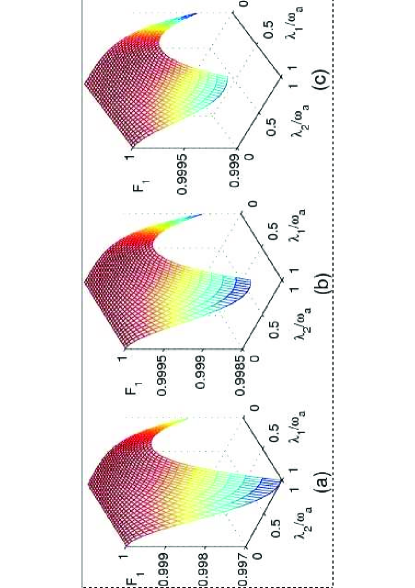
Figure 2: (Color online) The fidelity $F_{1}$ of the ground state for the single-qubit ASRM obtained by the transformation method versus the coupling strengths $\lambda_{1}$ and $\lambda_{2}$: (a) $w_{b}=0.8w_{a}$; (b) $w_{b}=w_{a}$; (c) $w_{b}=1.2w_{a}$.

II.2 Ground-state entanglement

In this section, we focus on the entanglement between the qubit and the oscillator in the ground state of the single-qubit ASRM. Since the ground state is a pure state, we take the von Neumann entropy as an entanglement measure. If a pure state of a composite system $XY$ is given by the density matrix $\rho_{XY}$, the entropy of the subsystem $X$ is defined as:

$$S_{\rho_{X}}=-Tr(\rho_{X}log_{2}\rho_{X}),$$ (29)

where $\rho_{X}=Tr_{Y}(\rho_{XY})$ is the reduced density matrix for the subsystem $X$ by tracing out the freedom degree of the subsystem $Y$. Note that $S_{\rho_{X}}$ measures the entanglement between the subsystems $X$ and $Y$ of the system, which has a maximum value of $log_{2}K$ in a $K$-dimensional Hilbert space.

In the standard basis $\{|\uparrow\rangle_{A},|\downarrow\rangle_{A}\}$, the reduced density matrix of the qubit is $\rho_{A}=Tr_{F}(|\Phi_{G}\rangle\langle\Phi_{G}|)$, where $|\Phi_{G}\rangle$ is the exactly numerical ground state of the single-qubit ASRM. The entropy of the qubit $S_{\rho_{A}}$ = $-Tr(\rho_{A}log_{2}\rho_{A})$ is numerically plotted in Fig. 3, which shows that the entanglement between the qubit and the oscillator increases from as $\lambda_{1}$ and $\lambda_{2}$ increase from zero to values close to $w_{a}$ and $w_{b}$.

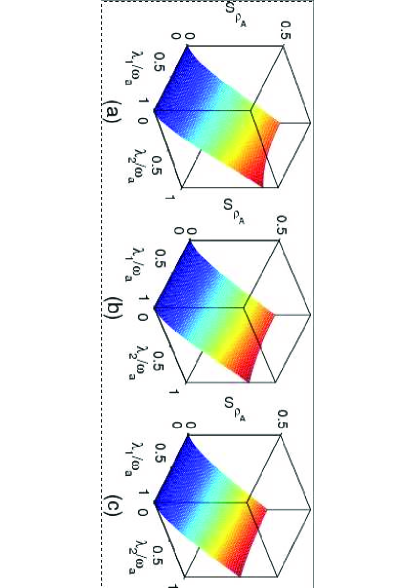
Figure 3: (Color online) The degree of entanglement $S_{\rho_{A}}$ for the qubit in the ground state of the single-qubit ASRM obtained by the numerical simulation versus the coupling strengths $\lambda_{1}$ and $\lambda_{2}$: (a) $w_{b}=0.8w_{a}$; (b) $w_{b}=w_{a}$; (c) $w_{b}=1.2w_{a}$.

III The two-qubit ASRM

III.1 Transformed ground state

The Hamiltonian of the two-qubit ASRM is PRA-8-1440-1973 :

$$H = w_{a}J_{z}+w_{b}b^{\dagger}b+g_{1}(b^{\dagger}J_{-}+bJ_{+})$$ (32)

$$+g_{2}(b^{\dagger}J_{+}+bJ_{-}),$$

where $w_{a}$ is the frequency of each qubit. $J_{l}\{l=x,y,z,\pm\}$ describes the collective qubit operator of a spin-$1$ system. $b^{\dagger}$ ($b$) is the creation (annihilation) operator of the harmonic oscillator with the frequency $w_{b}$. The qubit-oscillator coupling strengths of the corotating-wave and counterrotating-wave interactions are $g_{1}$ and $g_{2}$, respectively. We denote the eigenstates of $J_{z}$ by $|-1\rangle_{A}$, $|0\rangle_{A}$, and $|1\rangle_{A}$, i.e., $J_{z}|m\rangle_{A}=m|m\rangle_{A}$ ($m=0,\pm 1$). $|0\rangle_{F}$ is the vacuum state of the harmonic oscillator, and $|\alpha\rangle_{F}$ denotes the coherent-state field with the amplitude $\alpha$. When a rotation around the $y$ axis is performed, the Hamiltonian of the two-qubit ASRM can be written as :

$$H_{2} = w_{a}J_{x}+w_{b}b^{\dagger}b+(g_{1}+g_{2})(b^{\dagger}+b)J_{z}$$ (35)

$$+i(g_{1}-g_{2})(b^{\dagger}-b)J_{y}.$$

To transform the Hamiltonian $H_{2}$ into a mathematical form without counterrotating-wave terms, we apply a unitary transformation to $H_{2}$:

$$H_{2}^{{}^{\prime}} = e^{S_{2}}H_{2}e^{-S_{2}},$$ (36)

with

$$S_{2} = \xi_{2}(b^{\dagger}-b)J_{z},$$ (37)

where $\xi_{2}$ is a variable to be determined. Therefore, the transformed Hamiltonian $H_{2}^{{}^{\prime}}$ is decomposed into three parts:

$$H_{2}^{{}^{\prime}} = H_{2}^{a}+H_{2}^{b}+H_{2}^{c},$$ (38)

with

$$H_{2}^{a} = w_{b}b^{\dagger}b+\bigg{[}w_{a}\eta_{2}-(g_{1}-g_{2})\eta_{2}\xi_{2}\bigg{]}J_{x}$$ (40)

$$+\bigg{[}w_{b}\xi_{2}^{2}-2\xi_{2}(g_{1}+g_{2})\bigg{]}J_{z}^{2},$$

$$H_{2}^{b} = \bigg{[}(g_{1}+g_{2})-w_{b}\xi_{2}\bigg{]}(b^{\dagger}+b)J_{z}$$ (42)

$$+i\bigg{[}w_{b}\eta_{2}\xi_{2}+(g_{1}-g_{2})\eta_{2}\bigg{]}(b^{\dagger}-b)J_{y},$$

$$H_{2}^{c} = w_{a}J_{x}\bigg{\{}\cosh[\xi_{2}(b^{\dagger}-b)]-\eta_{2}\bigg{\}}$$ (47)

$$+iw_{a}J_{y}\bigg{\{}\sinh[\xi_{2}(b^{\dagger}-b)]-\eta_{2}\xi_{2}(b^{\dagger}-b)\bigg{\}}$$

$$+(g_{1}-g_{2})(b^{\dagger}-b)J_{x}\bigg{\{}\sinh[\xi_{2}(b^{\dagger}-b)]$$

$$-\eta_{2}\xi_{2}(b^{\dagger}-b)\bigg{\}}+i(g_{1}-g_{2})(b^{\dagger}-b)J_{y}$$

$$\times\bigg{\{}\cosh[\xi_{2}(b^{\dagger}-b)]-\eta_{2}\bigg{\}}+O(b^{\dagger 2},b^{2}),$$

where $\eta_{2}=$ ${}_{F}\langle 0|\cosh[\xi_{2}(b^{\dagger}-b)]|0\rangle_{F}$ $=$ $e^{-\xi_{2}^{2}/2}$ and $O(b^{\dagger 2},b^{2})=(g_{1}-g_{2})\eta_{2}\xi_{2}J_{x}(b^{\dagger 2}-2b^{\dagger}b-b^{2})$. As shown in the single-qubit ASRM, when $\xi_{2}$ and $|g_{1}\pm g_{2}|$ are much smaller than the frequency sum $w_{a}+w_{b}$ where $w_{a}\approx w_{b}$, $H_{2}^{c}$ can be neglected, thus $H_{2}^{{}^{\prime}}\simeq H_{2}^{a}+H_{2}^{b}$. Compared with $H_{1}^{a}$ in the single-qubit ASRM of Sec. II, the main difference is the presence of the $J_{z}^{2}$ operator term in $H_{2}^{a}$, but in the single-qubit ASRM the corresponding term $\sigma_{z}^{2}=1$ is just a constant. Therefore, $H_{2}^{a}$ here represents a renormalized three-level system in which we need to diagonalize $H_{2}^{a}$ to remove counterrotating-wave terms.

The eigenvalues $\nu_{k}$ ($k=1,2,3$) and eigenstates $|\varphi_{k}\rangle_{A}$ of the Hamiltonian $H_{2}^{{}^{\prime\prime}}=H_{2}^{a}-w_{b}b^{\dagger}b$ are:

$$\nu_{1} = \frac{A}{2}-\frac{1}{2}\sqrt{A^{2}+8B^{2}},$$ (48)

$$|\varphi_{1}\rangle_{A} = \frac{1}{N_{1}}\bigg{\{}|-1\rangle_{A}-\frac{(A+\sqrt{A^{2}+8B^{2}})}{2B}|0\rangle_{A}+|1\rangle_{A}\bigg{\}},$$ (49)

$$\nu_{2} = A,$$ (51)

$$|\varphi_{2}\rangle_{A} = \frac{1}{N_{2}}\bigg{\{}-|-1\rangle_{A}+|1\rangle_{A}\bigg{\}},$$ (53)

$$\nu_{3} = \frac{A}{2}+\frac{1}{2}\sqrt{A^{2}+8B^{2}},$$ (55)

$$|\varphi_{3}\rangle_{A} = \frac{1}{N_{3}}\bigg{\{}|-1\rangle_{A}-\frac{(A-\sqrt{A^{2}+8B^{2}})}{2B}|0\rangle_{A}+|1\rangle_{A}\bigg{\}},$$ (57)

with

$$A = w_{b}\xi_{2}^{2}-2\xi_{2}(g_{1}+g_{2}),$$ (59)

$$B = \frac{1}{\sqrt{2}}[w_{a}\eta_{2}-\eta_{2}\xi_{2}(g_{1}-g_{2})],$$ (60)

where $N_{k}$ is the normalization factor of the eigenvector $|\varphi_{k}\rangle_{A}$. Here the eigenvalues are arranged in the decreasing order: $\nu_{1}<\nu_{2}<\nu_{3}$. Then $H_{2}^{{}^{\prime}}$ can be expanded in terms of the renormalized eigenvectors:

$$H_{2}^{{}^{\prime}} \simeq \sum_{k=1}^{3}\nu_{k}|\varphi_{k}\rangle_{A}\langle\varphi_{k}|+\bigg{[}(D_{1}b+D_{2}b^{\dagger})|\varphi_{1}\rangle_{A}\langle\varphi_{2}|$$ (62)

$$+(D_{3}b+D_{4}b^{\dagger})|\varphi_{2}\rangle_{A}\langle\varphi_{3}|+H.c.\bigg{]}+w_{b}b^{\dagger}b,$$

where $D_{x}\ (x=1,2,3,4)$ is the coefficient depending on the variable $\xi_{2}$.

After transforming the Hamiltonian $H_{2}$ into $H_{2}^{{}^{\prime}}$, we can eliminate counterrotating-wave terms describing the coupling between the lowest two eigenstates by setting:

$$D_{1} = \eta_{2}\bigg{[}w_{a}\xi_{2}+(g_{1}-g_{2})\bigg{]}\bigg{(}A+\sqrt{A^{2}+8B^{2}}\bigg{)}$$ (64)

$$-2\sqrt{2}B\bigg{[}(g_{1}+g_{2})-w_{b}\xi_{2}\bigg{]}=0.$$

The value of $\xi_{2}$ is obtained by numerically solving the nonlinear equation (64). We find that when $g_{1}\leq 0.5w_{a}$ and $g_{2}\leq 0.5w_{a}$, $\xi_{2}$ has an approximately linear dependence on the coupling strengths:

$$\xi_{2} \simeq \frac{(w_{b}-w_{a})g_{1}+(w_{b}+w_{a})g_{2}}{w_{b}^{2}+w_{a}^{2}}.$$ (65)

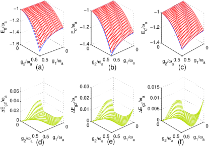
Figure 4: (Color online) The ground-state energy for the two-qubit ASRM obtained by the transformation method $E_{0}=E_{g2}$ (red grid) and the numerical solution $E_{0}=E_{g}$ (blue grid) versus the coupling strengths $g_{1}$ and $g_{2}$: (a) $w_{b}=0.8w_{a}$; (b) $w_{b}=w_{a}$; (c) $w_{b}=1.2w_{a}$, where $E_{g2}$ is plotted by using $\nu_{1}$ in Eq. (48). The energy deviation $\Delta E_{g2}=E_{g2}-E_{g}$ versus $g_{1}$ and $g_{2}$: (d) $w_{b}=0.8w_{a}$; (e) $w_{b}=w_{a}$; (f) $w_{b}=1.2w_{a}$.

In Fig. 4, we compare the ground-state energy obtained by the transformation method and that obtained by the numerical solution. We find that when $g_{1}\leq 0.25w_{a}$ and $g_{2}\leq 0.25w_{a}$, the ground-state energy obtained by the transformation method coincides very well with the exact value even for $|g_{1}-g_{2}|=0.24w_{a}$. Therefore, when $g_{1}\leq 0.5w_{a}$ and $g_{2}\leq 0.5w_{a}$, $|\varphi_{1}\rangle_{A}|0\rangle_{F}$ is expected to be the approximately analytical ground state of the transformed Hamiltonian, and the ground state $|\phi_{g}\rangle$ of the two-qubit ASRM can be expressed by the transformed ground state $|\phi_{g2}\rangle$:

$$|\phi_{g2}\rangle = e^{-S_{2}}|\varphi_{1}\rangle_{A}|0\rangle_{F}$$ (67)

$$=\frac{1}{N_{1}}\big{(}|-1\rangle_{A}|\xi_{2}\rangle_{F}-\frac{\nu_{3}}{B}|0\rangle_{A}|0\rangle_{F}+|1\rangle_{A}|-\xi_{2}\rangle_{F}\big{)},$$

and the ground-state energy $E_{g2}$ is:

$$E_{g2} \simeq \nu_{1}\simeq-w_{a}-\frac{(g_{1}+g_{2})g_{2}}{w_{a}w_{b}},$$ (69)

which directly shows that $E_{g2}$ has an approximately quadratic dependence on the qubit-oscillator coupling strengths by neglecting high-order terms of the field mode. This result differs further from that in the two-qubit SRM arXiv-1303-3367v2-2013 .

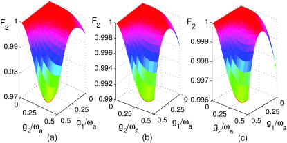
Figure 5: (Color online) The fidelity $F_{2}$ of the ground state for the two-qubit ASRM obtained by the transformation method versus the coupling strengths $g_{1}$ and $g_{2}$: (a) $w_{b}=0.8w_{a}$; (b) $w_{b}=w_{a}$; (c) $w_{b}=1.2w_{a}$.

The fidelity $F_{2}$ of the ground state as a function of the qubit-oscillator coupling strengths $g_{1}$ and $g_{2}$ under different detunings is plotted in Fig. 5. The result shows that $F_{2}$ keeps higher than $99.9\%$ when $g_{1}\leq 0.25w_{a}$ and $g_{2}\leq 0.25w_{a}$, which coincides with the behavior of the transformed ground-state energy shown in Fig. 5.

III.2 Ground-state entanglement

We also examine the ground-state entanglement of the two-qubit ASRM by taking into account both the transformation method and the exactly numerical treatment. Negativity is taken to quantify the entanglement for two qubits, which is defined as PRA-65-032314-2002 :

$$M_{\rho_{A}} = \frac{\|\rho_{A}^{T}\|-1}{2},$$ (70)

where $\rho_{A}^{T}$ is the partially transposed matrix of the two-qubit reduced density matrix $\rho_{A}$, with $\rho_{A}=Tr_{F}(\rho_{AF})$ and $\rho_{AF}=|\phi_{g}\rangle\langle\phi_{g}|$, and $\|\rho_{A}^{T}\|$ is the trace norm of $\rho_{A}^{T}$. Thus, $M_{\rho_{A}}$ alternatively equals the absolute value for the sum of the negative eigenvalues of $\rho_{A}^{T}$. For the transformed ground state $|\phi_{g2}\rangle$ in Eq. (67), the partially transposed matrix of the reduced density operator for the two qubits in the qubit basis $\Gamma_{q}$ $=$ $\{$ $|\uparrow_{1}\rangle|\uparrow_{2}\rangle,|\uparrow_{1}\rangle|\downarrow_{2}\rangle,|\downarrow_{1}\rangle|\uparrow_{2}\rangle,|\downarrow_{1}\rangle|\downarrow_{2}\rangle$ $\}$, where $|\uparrow_{l}\rangle$ and $|\downarrow_{l}\rangle$ ($l=1,2$) correspond to the excited and ground states of the $l$th qubit respectively, is obtained as follows:

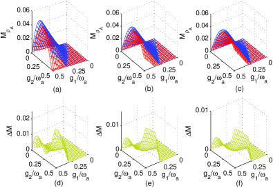
Figure 6: (Color online) The negativity $M_{\rho_{A}}$ of two qubits in the ground state of the two-qubit ASRM versus the coupling strengths $g_{1}$ and $g_{2}$: (a) $w_{b}=0.8w_{a}$; (b) $w_{b}=w_{a}$; (c) $w_{b}=1.2w_{a}$. The results obtained by the transformation method $M_{\rho_{A}}=M_{\rho_{A}}^{t}$ and the numerical simulation $M_{\rho_{A}}=M_{\rho_{A}}^{n}$ are represented by the red grid and the blue grid, respectively. The deviation in the two-qubit negativity $\Delta M=M_{\rho_{A}}^{n}-M_{\rho_{A}}^{t}$ obtained by transformation method: (d) $w_{b}=0.8w_{a}$; (e) $w_{b}=w_{a}$; (f) $w_{b}=1.2w_{a}$.

$$\rho_{A}^{T} = \frac{1}{(2+\beta^{2})}\left(\begin{array}[]{cccc}1&\frac{\beta}{\sqrt{2}}e^{-\frac{\alpha^{2}}{2}}&\frac{\beta}{\sqrt{2}}e^{-\frac{\alpha^{2}}{2}}&\frac{\beta^{2}}{2}\\ \frac{\beta}{\sqrt{2}}e^{-\frac{\alpha^{2}}{2}}&\frac{\beta^{2}}{2}&e^{-2\alpha^{2}}&\frac{\beta}{\sqrt{2}}e^{-\frac{\alpha^{2}}{2}}\\ \frac{\beta}{\sqrt{2}}e^{-\frac{\alpha^{2}}{2}}&e^{-2\alpha^{2}}&\frac{\beta^{2}}{2}&\frac{\beta}{\sqrt{2}}e^{-\frac{\alpha^{2}}{2}}\\ \frac{\beta^{2}}{2}&\frac{\beta}{\sqrt{2}}e^{-\frac{\alpha^{2}}{2}}&\frac{\beta}{\sqrt{2}}e^{-\frac{\alpha^{2}}{2}}&1\end{array}\right),$$ (75)

where $\alpha=\xi_{2}$ and $\beta=-\frac{\nu_{3}}{B}$. With Eq. (75), we can calculate the negative $M_{\rho_{A}}$:

$$M_{\rho_{A}} = \max\bigg{\{}\frac{2e^{-2\xi_{2}^{2}}-(\frac{\nu_{3}}{B})^{2}}{2[2+(\frac{\nu_{3}}{B})^{2}]},0\bigg{\}}.$$ (77)

When $g_{1}\leq 0.25w_{a}$ and $g_{2}\leq 0.25w_{a}$, $M_{\rho_{A}}$ approximates:

$$M_{\rho_{A}} \simeq \frac{w_{b}\big{[}(1-\frac{1}{\sqrt{2}})^{2}g_{2}^{2}+g_{1}g_{2}\big{]}}{4w_{a}(w_{a}+w_{b})^{2}}.$$ (78)

From Eq. (78), we see that the two-qubit entanglement increases with $g_{2}^{2}$ and $g_{1}g_{2}$. The two-qubit negativity as a function of the qubit-oscillator coupling strengths $g_{1}$ and $g_{2}$ under different detunings has been plotted in Fig. 6 (a) - (c), and the corresponding deviation from the numerical simulation is plotted in Fig. 6 (d) - (f). For $0<g_{1}\leq 0.25w_{a}$ and $0<g_{2}\leq 0.25w_{a}$, the two-qubit negativity has a linear dependence on $g_{1}$ for the fixed $g_{2}$ and a quadratic dependence on $g_{2}$ for the fixed $g_{1}$; For $0<g_{1}\leq 0.25w_{a}$ and $0.25w_{a}<g_{2}<0.5w_{a}$, the negativity keeps close to zero; However, for $0.25w_{a}<g_{1}<0.5w_{a}$ and $0<g_{2}<0.5w_{a}$, the negative has a similar dependence on $g_{1}$ and $g_{2}$ with the case of $0<g_{1}\leq 0.25w_{a}$ and $0<g_{2}\leq 0.25w_{a}$. We find that when $g_{1}\leq 0.25w_{a}$ and $g_{2}\leq 0.25w_{a}$ the deviation in the negativity is close to zero, meaning the ground state obtained by the transformation method agrees well with the exact one. This directly shows that the two-qubit entanglement is caused by the counterrotating-wave interaction in the Hamiltonian. Interestingly, after the negativity has reached its maximum, it will monotonically decrease when $g_{1}$ or $g_{2}$ further increases. Furthermore, the maximum of the two-qubit entanglement in the two-qubit ASRM is far larger than that in the two-qubit SRM, and the two-qubit entanglement mainly appears when the coupling strength of the corotating-wave interaction is bigger than that of the counterrotating-wave interaction, which is because the contribution to the two-qubit entanglement from the counterrotating-wave interaction is larger than that from the corotating-wave interaction in Eq. (78). As seen from Fig. 7, when $g_{1}>1.11w_{a}$ or $g_{2}>0.88w_{a}$ at $w_{b}=w_{a}$, $M_{\rho_{A}}$ decreases to zero and never increases again, and the maximum negativity is about $0.10$ which is only $3.5\times 10^{-2}$ in the two-qubit SRM arXiv-1303-3367v2-2013 .

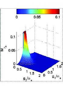
Figure 7: (Color online) The negativity $M_{\rho_{A}}$ of two qubits in the ground state of the two-qubit ASRM obtained by the numerical simulation versus the coupling strengths $g_{1}$ and $g_{2}$ when $w_{b}=w_{a}$.

In Fig. 8, we numerically plot the entropy $S_{\rho_{A}}$ of two qubits versus the coupling strengths $g_{1}$ and $g_{2}$ in the ground state of the two-qubit ASRM, where $S_{\rho_{A}}$ $=$ $-Tr(\rho_{A}log_{2}\rho_{A})$. The result shows that the entanglement between the qubit and the oscillator increases from as $g_{1}$ and $g_{2}$ increase from zero to values close to $w_{a}$ and $w_{b}$.

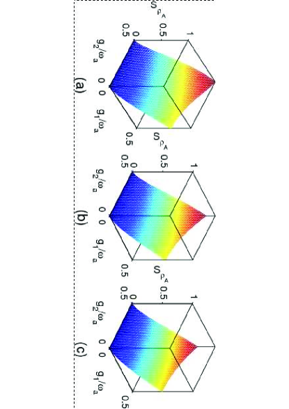
Figure 8: (Color online) The degree of entanglement $S_{\rho_{A}}$ for the qubits in the ground state of the two-qubit ASRM obtained by numerical simulations versus the coupling strengths $g_{1}$ and $g_{2}$: (a) $w_{b}=0.8w_{a}$; (b) $w_{b}=w_{a}$; (c) $w_{b}=1.2w_{a}$.

IV Conclusion

In conclusion, we have used the transformation method to obtain the approximately analytical ground states of the single- and two-qubit ASRMs, and shown that the transformed results coincided well with those obtained by numerical simulations for a wide range of parameters under the near-resonance condition. We find that the ground-state energy in either the single- or two-qubit ASRM has an approximately quadratic dependence on the qubit-oscillator coupling strengths, and the contribution of the counterrotating-wave interaction on the ground state energy is larger than that of the corotating-wave interaction. Interestingly, we also find that the two-qubit entanglement of the two-qubit ASRM decreases to zero and never increases again as long as the qubit-oscillator coupling strengths are large enough. Furthermore, the maximum of the two-qubit entanglement in the two-qubit ASRM is far larger than that in the two-qubit SRM, and the two-qubit entanglement mainly appears when the coupling strength of the corotating-wave interaction is bigger than that of the counterrotating-wave interaction.

V Acknowledgement

This work is supported by the Major State Basic Research Development Program of China under Grant No. 2012CB921601, the National Natural Science Foundation of China under Grant No. 11374054, No. 11305037, No. 11347114, and No. 11247283, the Natural Science Foundation of Fujian Province under Grant No. 2013J01012, and the funds from Fuzhou University under Grant No. 022513, Grant No. 022408, and Grant No. 600891.

References

- (1) I. I. Rabi, Phys. Rev. 49, 324 (1936); 51, 652 (1937).
- (2) E. T. Jaynes and F. W. Cummings, Proc. IEEE 51, 89 (1963). S. B. Zheng and G. C. Guo, Phys. Rev. Lett. 85, 2392 (2000).
- (3) B. W. Shore and P. L. Knight, J. Mod. Opt. 40, 1195 (1993).
- (4) S. Osnaghi, P. Bertet, A. Auffeves, et al., Phys. Rev. Lett. 87, 037902 (2001).
- (5) S. M. Spillane, T. J. Kippenberg, K. J. Vahala, et al., Phys. Rev. A 71, 013817 (2005); Y. Wu and X. Yang, Phys. Rev. Lett. 78, 3086 (1997); X. Yang, Y. Wu, and Y. J. Li, Phys. Rev. A 55, 4545 (1997).
- (6) J. Q. You and F. Nori, Physics Today 58, 42-47 (2005).
- (7) I. Buluta and F. Nori, Science 326, 108-111 (2009).
- (8) S. N. Shevchenko, S. Ashhab, and F. Nori, Physics Reports 492, 1-30 (2010).
- (9) I. Buluta, S. Ashhab, and F. Nori, Rep. Prog. Phys. 74, 104401 (2011).
- (10) J. Q. You and F. Nori, Nature 474, 589 (2011).
- (11) P. D. Nation, J. R. Johansson, M. P. Blencowe, and F. Nori, Rev. Mod. Phys. 84, 1-24 (2012).
- (12) Z. L. Xiang, S. Ashhab, J. Q. You, and F. Nori, Rev. Mod. Phys. 85, 623 (2013).
- (13) I. M. Georgescu, S. Ashhab, and F. Nori, Rev. Mod. Phys. 86, 153 (2014).
- (14) A. A. Abdumalikov Jr, O. Astafiev, Y. Nakamura, Y. A. Pashkin, and J. S. Tsai, Phys. Rev. B 78, 180502(R) (2008).
- (15) A. A. Anappara, S. D. Liberato, A. Tredicucci, C. Ciuti, G. Biasiol, L. Sorba, and F. Beltram, Phys. Rev. B 79, 201303(R) (2009).
- (16) G. Günter, A. A. Anappara, J. Hees, et al., Nature 458, 178 (2009).
- (17) T. Niemczyk, F. Deppe, H. Huebl, et al., Nature 6, 772 (2010).
- (18) P. Forn-Díaz, J. Lisenfeld, D. Marcos, J. J. García-Ripoll, E. Solano, C. J. P. M. Harmans, and J. E. Mooij, Phys. Rev. Lett. 105, 237001 (2010).
- (19) Y. Todorov, A. M. Andrews, R. Colombelli, et al., Phys. Rev. Lett. 105, 196402 (2010).
- (20) T. Schwartz, J. A. Hutchison, C. Genet, and T. W. Ebbesen, Phys. Rev. Lett. 106, 196405 (2011).
- (21) G. Scalari, C. Maissen, D. Turčinková, et al. Science 335, 1323 (2012).
- (22) A. Crespi, S. Longhi, and R. Osellame, Phys. Rev. Lett. 108, 163601 (2012).
- (23) S. Hayashi, Y. Ishigaki, and M. Fujii, Phys. Rev. B 86, 045408 (2012).
- (24) J. Li, M. P. Silveri, K. S. Kumar, J. M. Pirkkalainen, A. Vepsäläinen, W. C. Chien, J. Tuorila, M. A. Sillanpää, P. J. Hakonen, E. V. Thuneberg, G. S. Paraoanu, Nature Communications 4, 1420 (2013).
- (25) X. Cao, J. Q. You, H. Zheng, and F. Nori, New J. Phys. 13, 073002 (2011).
- (26) A. Ridolfo, M. Leib, S. Savasta, and M. J. Hartmann, Phys. Rev. Lett. 109, 193602 (2012).
- (27) S. Ashhab and F. Nori, Phys. Rev. A 81, 042311 (2010).
- (28) S. Ashhab, Phys. Rev. A 87, 013826 (2013).
- (29) H. P. Zheng, F. C. Lin, Y. Z. Wang, and Y. Segawa, Phys. Rev. A 59, 4589 (1999).
- (30) S. B. Zheng, X. W. Zhu, and M. Feng, Phys. Rev. A 62, 033807 (2000).
- (31) E. K. Irish, J. Gea-Banacloche, I. Martin, and K. C. Schwab, Phys. Rev. B 72, 195410 (2005).
- (32) C. Ciuti and I. Carusotto, Phys. Rev. A 74, 033811 (2006).
- (33) D. Wang, T. Hansson, Å. Larson, H. O. Karlsson, and J. Larson, Phys. Rev. A 77, 053808 (2008).
- (34) X. F. Cao, J. Q. You, H. Zheng, A. G. Kofman, and F. Nori, Phys. Rev. A 82, 022119 (2010).
- (35) P. Nataf and C. Ciuti, Phys. Rev. Lett. 107, 190402 (2011).
- (36) V. V. Albert, Phys. Rev. Lett. 108, 180401 (2012).
- (37) X. F. Cao, Q. Ai, C. P. Sun, and F. Nori, Phys. Lett. A 376, 349 (2012).
- (38) I. D. Feranchuk, L. I. Komarov, and A. P. Ulyanenkov, J. Phys. A: Math. Gen. 29, 4035 (1996).
- (39) Q. H. Chen, T. Liu, Y. Y. Zhang, and K. L. Wang, Eur. Phys. Lett. 96, 14003 (2011).
- (40) H. Chen, Y. M. Zhang, and X. Wu, Phys. Rev. B 40, 11326 (1989).
- (41) J. Stolze and L. Müller, Phys. Rev. B 42, 6704 (1990).
- (42) E. K. Irish, Phys. Rev. Lett. 99, 173601 (2007).
- (43) T. Liu, K. L. Wang, and M. Feng, Eur. Phys. Lett. 86, 54003 (2009).
- (44) D. Zueco, G. M. Reuther, S. Kohler, and P. Hänggi, Phys. Rev. A 80, 033846 (2009).
- (45) J. Casanova, G. Romero, I. Lizuain, J. J. García-Ripoll, and E. Solano, Phys. Rev. Lett. 105, 263603 (2010).
- (46) M. J. Hwang and M. S. Choi, Phys. Rev. A 82, 025802 (2010).
- (47) J. Song, Y. Xia, X. D. Sun, Y. Zhang, B. Liu, and H. S. Song, Eur. Phys. J. D 66, 1 (2012).
- (48) L. X. Yu, S. Q. Zhu, Q. F. Liang, G. Chen, and S. T. Jia, Phys. Rev. A 86, 015803 (2012).
- (49) S. Agarwal, S. M. H. Rafsanjani, and J. H. Eberly, Phys. Rev. A 85, 043815 (2012).
- (50) Q. H. Chen, C. Wang, S. He, T. Liu, and K. L. Wang, Phys. Rev. A 86, 023822 (2012).
- (51) H. Zheng, Eur. Phys. J. B 38, 559 (2004).
- (52) Z. G. Lü and H. Zheng, Phys. Rev. B 75, 054302 (2007).
- (53) C. J. Gan and H. Zheng, Eur. Phys. J. D 59, 473 (2010).
- (54) K. M. C. Lee and C. K. Law, Phys. Rev. A 88, 015802 (2013).
- (55) L. T. Shen, Z. B. Yang, and R. X. Chen, Phys. Rev. A 88, 045803 (2013).
- (56) F. Altintas and R. Eryigit, Phys. Rev. A 87, 022124 (2013).
- (57) L. H. Du, X. F. Zhou, Z. W. Zhou, X. Zhou, and G. C. Guo, Phys. Rev. A 86, 014303 (2012).
- (58) H. H. Zhong, Q. T. Xie, and C. H. Lee, J. Phys. A: Math. Theor. 46, 415302 (2013); G. H. Tian and S. Q. Zhong, arXiv:1309.7715v1, (2013).
- (59) D. Braak, Phys. Rev. Lett. 107, 100401 (2011).
- (60) F. Dimer, B. Estienne, A. S. Parkins, and H. J. Carmichael, Phys. Rev. A 75, 013804 (2007); A. L. Grimsmo and S. Parkins, Phys. Rev. A 87, 033814 (2013).
- (61) F. T. Hioe, Phys. Rev. A 8, 1440 (1973).
- (62) G. Vidal, R. F. Werner, Phys. Rev. A 65, 032314 (2002).