Effect of dot size on exciton binding energy and electron-hole recombination probability in CdSe quantum dots

Abstract

  Exciton binding energy and electron-hole recombination probability are presented as the two important metrics for investigating effect of dot size on electron-hole interaction in CdSe quantum dots. Direct computation of electron-hole recombination probability is challenging because it requires an accurate mathematical description of electron-hole wavefunction in the neighborhood of the electron-hole coalescence point. In this work, we address this challenge by solving the electron-hole Schrodinger equation using the electron-hole explicitly correlated Hartree-Fock (eh-XCHF) method. The calculations were performed for a series of CdSe clusters ranging from $\mathrm{Cd}_{20}\mathrm{Se}_{19}$ to $\mathrm{Cd}_{74608}\mathrm{Se}_{74837}$ that correspond to dot diameter range of $1-20$ nm. The calculated exciton binding energies and electron-hole recombination probabilities were found to decrease with increasing dot size. Both of these quantities were found to scale as $D_{\mathrm{dot}}^{-n}$ with respect to the dot diameter D. One of the key insights from this study is that the electron-hole recombination probability decreases at a much faster rate than the exciton binding energy as a function of dot size. It was found that an increase in the dot size by a factor of 16.1, resulted in a decrease in the exciton binding energy and electron-hole recombination probability by a factor of 14.4 and $5.5\times 10^{6}$, respectively.  

I Introduction

Semiconductor quantum dots and rods have been the focus of intense theoretical and experimental research because of inherent size-dependent optical and electronic properties. Generation of bound electron-hole pairs (excitons) and dissociation of excitons into free charge carriers are the two important factors that directly impact the light-harvesting efficiency of the semiconductor quantum dots. The dissociation of excitons is a complex process that is influenced by various factors such as shape and size of the quantum dots, Zhu and Lian (2012); Ghosh et al. (2012); Bae et al. (2013); Lin et al. (2011); Alam et al. (2012); Han et al. (2010) presence of surface defects, Williams et al. (2013); Yin et al. (2013); Jaeger et al. (2012) surface ligands, Kilina et al. (2012, 2009a) and coupling with phonon modes. Kilina et al. (2009b); Kelley (2010, 2011); Kelley et al. (2012); Kilina et al. (2011); Hyeon-Deuk and Prezhdo (2011, 2012a); Kilina et al. (2013) The energetics of the electron-hole interaction in quantum dots is quantified by the exciton dissociation energy and has been determined using both theoretical and experimental techniques Musa et al. (2011); Chon et al. (2011); Franceschetti and Zunger (2001). Generation of free charge carrier by exciton dissociated has been facilitated by introducing core/shell heterojunctions Zhu et al. (2011, 2010); Hoy et al. , and applying external and ligand-induced electric fields. Li et al. (2012); Yaacobi-Gross et al. (2011); Liu et al. (2012); Perebeinos and Avouris (2007); Blanton et al. (2013); Park et al. (2012)

One of the direct routes for enhancing exciton dissociation is by modifying the size and shape of quantum dots. Studies on CdSe and other quantum dots have shown that the exciton binding energy decreases with increasing dot size. Franceschetti and Zunger (1997); Meulenberg et al. (2009); Jasieniak et al. (2011); Maan et al. (1984); Ramvall et al. (1998); Wang and Zunger (1996); Kucur et al. (2003); Inamdar et al. (2008); Querner et al. (2005) The size of the quantum dots have significant impact on the Auger recombination, García-Santamaría et al. (2009); Wang et al. (2003) multiple exciton generation Hyeon-Deuk and Prezhdo (2012b); Rabani and Baer (2010); Lin et al. (2011); Jaeger et al. (Article ASAP), and blinking effect in quantum dots Vela et al. (2010); Bae et al. (2013); Ghosh et al. (2012). In addition to exciton binding energy, the spatial distribution of electrons and holes in quantum dots also provides important insight into the exciton dissociation process. Rawalekar et al. (2010); Nemchinov et al. (2008) Electron and hole densities $\rho_{\mathrm{e}}(\mathbf{r})$ and $\rho_{\mathrm{h}}(\mathbf{r})$ have been widely used to investigate quasi-particle distribution in quantum dots. Zhu et al. (2011, 2010) For example in core/shell quantum dots, presence of the heterojunction induces asymmetric spatial distribution of electrons and holes which, in turn, facilitates the exciton dissociation. Asymmetric electron probability density in the shell region of the core/shell quantum dots has been attributed to fast electron transfer from the quantum dots. Zhu et al. (2011, 2010); Yan et al. (2011); Xu et al. (2012)

The central challenge in the theoretical investigation of quantum dots is efficient computational treatment of large number of electrons in the system. For small clusters where all-electron treatment is feasible, ground state and excited-state calculations have been performed using GW Bethe-Salpeter, Noguchi et al. (2012); Lopez Del Puerto et al. (2008); Del Puerto et al. (2006) density functional theory (DFT) Nguyen et al. (2010); Yang et al. (2011); Albert et al. (2011); Kilin et al. (2007); Liu et al. (2009); Chung et al. (2009); Kim et al. (2010), time-dependent DFT (TDDFT) Nadler and Sanz (2013); Abuelela et al. (2012); Fischer et al. (2012); Del Ben et al. (2011); Turkowski et al. (2009); Li and Ullrich (2011); Yang et al. (2012); Yang and Ullrich (2013), and MP2 Neuhauser et al. (2013). For bigger quantum dots where all-electron treatment is computationally prohibitive, atomistic semiemperical pseudopotential methods have been used extensively. Franceschetti and Zunger (1997); Wang and Zunger (1996); Franceschetti et al. (1999); Wang et al. (2003); Baer and Rabani (2013) In this approach, the one-particle Schrödinger equation incorporating the pseudopotential $v_{\mathrm{ps}}$

$$\left[-\frac{\hbar^{2}}{2m}\nabla^{2}+v_{\mathrm{ps}}\right]\phi_{i}=\lambda_{i}\phi_{i},$$ (1)

is solved and the eigenfunctions are used in construction of the quasiparticle states Wang and Zunger (1996); Franceschetti and Zunger (1997). The quasiparticle states serve as a basis for both configuration interaction (CI) and perturbation theory calculations. Solution of Eq. (1) is generally obtained by introducing a set of basis functions (typically plane-waves), constructing the Hamiltonian matrix in that basis, and diagonalizing it. The computational efficiency of CI has been greatly improved by using only states near the band gap for construction of the CI space  Wang and Zunger (1996); Rabani et al. (1999). This technique alleviates the need to compute the entire eigenspectrum of the Hamiltonian matrix, however successful implementation of this approach requires computation of selected eigenvalues and eigenfunctions of the Hamiltonian matrix. Computation of the specific eigenvalues of large matrices is challenging and various methods such as the folded-spectrum method Wang and Zunger (1994); Canning et al. (2000), the filter-diagonalization method Toledo and Rabani (2002); Neuhauser et al. (2013), and generalized Davidson method Vömel et al. (2008); Jordan et al. (2012) have been specifically developed to address this problem.

The main goal of this article is to compare the effect of dot size on exciton binding energy and electron-hole recombination probability. The central quantity of interest for the present work is the electron-hole pair density $\rho(\mathbf{r}_{\mathrm{e}},\mathbf{r}_{\mathrm{h}})$. The electron-hole pair density is defined as the probability density of finding an electron and a hole in the neighborhood of $\mathbf{r}_{\mathrm{e}}$ and $\mathbf{r}_{\mathrm{h}}$, respectively. The pair density is a mathematically complicated quantity and is generally obtained from an underlying wavefunction. Direct construction of the pair-density is also possible as long as $N-\mathrm{representability}$ can be enforced Mazziotti (2007). For an interacting electron-hole system, the pair density is not equal to the product of electron and hole densities

$$\rho_{\mathrm{eh}}(\mathbf{r}_{\mathrm{e}},\mathbf{r}_{\mathrm{h}})\neq\rho_{\mathrm{e}}(\mathbf{r}_{\mathrm{e}})\rho_{\mathrm{h}}(\mathbf{r}_{\mathrm{h}}).$$ (2)

Furthermore, the electron-hole pair density contains information about the correlated spatial distribution of the electrons and hole that cannot be obtained from the product of individual electron and hole densities. Both electron-hole recombination probability and exciton binding energy can be computed directly from the pair density. The relationship between the exciton binding energy $E_{\mathrm{BE}}$ and electron-hole pair density is given by the following expression,

$$E_{\mathrm{BE}} =\int d\mathbf{r}_{\mathrm{e}}d\mathbf{r}_{\mathrm{h}}\,\,\rho_{\mathrm{eh}}(\mathbf{r}_{\mathrm{e}},\mathbf{r}_{\mathrm{h}})r^{-1}_{\mathrm{eh}}\epsilon^{-1}(\mathbf{r}_{\mathrm{e}},\mathbf{r}_{\mathrm{h}}),$$ (3)

where, $\epsilon^{-1}(\mathbf{r}_{\mathrm{e}},\mathbf{r}_{\mathrm{h}})$ is the inverse dielectric function. The electron-hole recombination probability, $P_{\mathrm{eh}}$ is related to the pair density as

$$P_{\mathrm{eh}} =\frac{1}{N_{\mathrm{e}}N_{\mathrm{h}}}\int d\mathbf{r}_{\mathrm{e}}\int_{\mathbf{r}_{\mathrm{e}}-\frac{\Delta}{2}}^{\mathbf{r}_{\mathrm{e}}+\frac{\Delta}{2}}d\mathbf{r}_{\mathrm{h}}\,\,\rho_{\mathrm{eh}}(\mathbf{r}_{\mathrm{e}},\mathbf{r}_{\mathrm{h}}),$$ (4)

where $N_{\mathrm{e}}$ and $N_{\mathrm{h}}$ are number of electron and holes, respectively. In the above equation, we define electron-hole recombination probability as the probability of finding a hole in a cube of volume $\Delta^{3}$ centered at the electron position. The computation of the recombination probability is especially demanding because it requires evaluation of the pair density at small interparticle distances. As a consequence, the form of the electron-hole wavefunction near the electron-hole coalescence point is very important. Elward et al. (2012a, b); Wimmer et al. (2006a); Cancio and Chang (1990, 1993); Zhu et al. (1996) In the present work, we address this challenge by using the electron-hole explicitly correlated Hartree-Fock (eh-XCHF) method. Elward et al. (2012a, b) The eh-XCHF method is a variational method where the wavefunction depends explicitly on the electron-hole interparticle distance and has been used successfully for investigating electron-hole interaction  Elward et al. (2012a, b); Blanton et al. (2013).

The remainder of the article is organized as follows. The theoretical details of the eh-XCHF and its computational implementation for CdSe quantum dots are presented in section II and section III, respectively. The results from the calculations are presented in section IV, and the conclusions from the study are discussed in section V.

II Theory

In the eh-XCHF method, Elward et al. (2012a, b) the electron-hole wavefunction is represented by multiplying the mean-field wavefunction with an explicitly correlated function as shown in the following equation

$$\Psi_{\mathrm{eh-XCHF}}=G\Phi^{\mathrm{e}}\Phi^{\mathrm{h}},$$ (5)

where $\Phi^{\mathrm{e}}$ and $\Phi^{\mathrm{h}}$ are electron and hole Slater determinants and $G$ is a Gaussian-type geminal (GTG) function Boys (1960) which is defined as,

$$G(\mathbf{r}^{\mathrm{e}},\mathbf{r}^{\mathrm{h}})=\sum_{i=1}^{N_{\mathrm{e}}}\sum_{j=1}^{N_{\mathrm{h}}}\sum_{k=1}^{N_{\mathrm{g}}}b_{k}\mathrm{exp}[-\gamma_{k}r^{2}_{ij}].$$ (6)

The GTG function depends on the $r_{\mathrm{eh}}$ term and is responsible for introduction of the electron-hole inter-particle distance dependence in the eh-XCHF wavefunction. The coefficients $b_{k}$ and $\gamma_{k}$ are expansion coefficients which are obtained variationally. The use of Gaussian-type geminal functions offers three principle advantages. First, the variational determination of the geminal parameters $\{b_{k},\gamma_{k}\}$ results in accurate description of the wavefunction near the electron-hole coalescence point. This feature is crucial for accurate computation of electron-hole recombination probability. Second, the integrals of GTG functions with Gaussian-type orbitals (GTO) can be performed analytically and have been derived earlier by BoysBoys (1960) and Persson et al. Persson and Taylor (1996) This alleviates the need to approximate the integrals using numerical methods. The third advantage of the GTG function is that it allows construction of a compact representation of an infinite-order configuration interaction expansion. This can be seen explicitly by introduction of the closure relationship,

$$G|\Psi_{\mathrm{ref}}\rangle =\underbrace{\sum_{ii^{\prime}}^{\infty}|\Phi^{\mathrm{e}}_{i}\Phi^{\mathrm{h}}_{i^{\prime}}\rangle\langle\Phi^{\mathrm{e}}_{i}\Phi^{\mathrm{h}}_{i^{\prime}}|}_{\mathbf{1}}G|\Psi_{\mathrm{ref}}\rangle.$$ (7)

The electron-hole interaction was described using the effective electron-hole HamiltonianHu et al. (1990); Zhu et al. (1996); Burovski et al. (2001); Wimmer et al. (2006b); Woggon (1997); Braskén et al. (2001); Corni et al. (2003a, b, c); Vänskä et al. (2006); Vänskä and Sundholm (2010); Sundholm and Vänskä (2012) which is defined in the following equation

$$H =\sum_{ij}\langle i|\frac{-\hbar^{2}}{2m_{\mathrm{e}}}+v_{\mathrm{ext}}^{\mathrm{e}}|j\rangle e_{i}^{\dagger}e_{j}$$ (8)

$$+\sum_{ij}\langle i|\frac{-\hbar^{2}}{2m_{\mathrm{h}}}+v_{\mathrm{ext}}^{\mathrm{h}}|j\rangle h^{\dagger}_{i}h_{j}$$

$$+\sum_{iji^{\prime}j^{\prime}}\langle iji^{\prime}j^{\prime}|\epsilon^{-1}r_{\mathrm{eh}}^{-1}|iji^{\prime}j^{\prime}\rangle e^{\dagger}_{i}e_{j}h_{i^{\prime}}^{\dagger}h_{j^{\prime}}$$

$$+\sum_{ijkl}w_{ijkl}^{\mathrm{ee}}e^{\dagger}_{i}e_{j}^{\dagger}e_{l}e_{k}+\sum_{ijkl}w_{ijkl}^{\mathrm{hh}}h^{\dagger}_{i}h_{j}^{\dagger}h_{l}h_{k}.$$

The effective electron-hole Hamiltonian provides a computationally efficient route for investigating large systems and in the present work was used for investigating CdSe clusters in the range of $\mathrm{Cd}_{20}\mathrm{Se}_{19}$ to $\mathrm{Cd}_{74608}\mathrm{Se}_{74837}$. We have also developed eh-XCHF method using a pseudopotential Elward and Chakraborty , but the current implementation is restricted to cluster sizes of 200 atoms and cannot be applied to large dot sizes.

The effective Hamiltonian in Eq. (8) was used in combination with parabolic potential which has been used extensively Halonen et al. (1992); El-Said (1994); Jaziri and Bennaceur (1994); Lamouche and Fishman (1998); Xie and Gu (2003); Xie (2005, 2009); Karimi and Rezaei (2011); Nammas et al. (2011); Rezaei et al. (2011) for approximating the confining potential in quantum dots and wires. The electron and hole external potentials $v^{\alpha}_{\mathrm{ext}}$ were expressed as

$$v^{\alpha}_{\mathrm{ext}}=\frac{1}{2}k_{\alpha}|\mathbf{r}_{\alpha}|^{2}\quad\alpha=\mathrm{e,h}.$$ (9)

The form of the external potential directly impacts the electron-hole pair density and is important for accurate computation of the binding energy and recombination probability. In this work, we have developed a particle number based search procedure for determining the external potential. The central idea of this method is to find an external potential such that the computed 1-particle electron and hole densities are spatially confined within the volume of the quantum dot. Mathematically, this is implemented by obtaining the force constant $k$ by the following minimization process

$$\min_{k_{\alpha}^{\mathrm{min}}}\left(N_{\alpha}-\int_{0}^{\frac{D_{\mathrm{dot}}}{2}}drr^{2}\int d\Omega\rho_{\alpha}(\mathbf{r})[v^{\alpha}_{\mathrm{ext}}]\right)^{2},$$ (10)

where $\alpha=\mathrm{e,h}$, $d\Omega=sin\theta d\theta d\phi$, $D_{\mathrm{dot}}$ is the dot diameter, and $k_{\alpha}^{\mathrm{min}}$ is the smallest force constant that satisfies the above minimization conditions. The single-particle density is a functional of the external potential and is denoted explicitly in the above equation.

The eh-XCHF wavefunction is obtained variationally by minimizing the eh-XCHF energy

$$E_{\mathrm{eh-XCHF}} =\min_{G,\Phi^{\mathrm{e}},\Phi^{\mathrm{h}}}\frac{\langle\Psi_{\mathrm{eh-XCHF}}|H|\Psi_{\mathrm{eh-XCHF}}\rangle}{\langle\Psi_{\mathrm{eh-XCHF}}|\Psi_{\mathrm{eh-XCHF}}\rangle}.$$ (11)

Instead of evaluating the above equation directly, it is more efficient to first transform the operators and then perform the integration over the coordinates. The transformed operators are obtained by performing congruent transformation Elward et al. (2012c); Bayne et al. which is defined as follows

$$\tilde{H}=G^{\dagger}HG$$ (12)

$$\tilde{1}=G^{\dagger}HG.$$ (13)

The eh-XCHF energy is obtained from the transformed operators using the following expression

$$E_{\mathrm{eh-XCHF}} =\frac{\langle\Phi^{\mathrm{e}},\Phi^{\mathrm{h}}|\tilde{H}|\Phi^{\mathrm{e}},\Phi^{\mathrm{h}}\rangle}{\langle\Phi^{\mathrm{e}},\Phi^{\mathrm{h}}|\tilde{1}|\Phi^{\mathrm{e}},\Phi^{\mathrm{h}}\rangle}.$$ (14)

The above equation allows us to reduce the minimization over the electron and hole Slater determinants in terms of coupled self-consistent field (SCF) equations as shown below Swalina et al. (2006)

$$\mathbf{F}_{G}^{\mathrm{e}}[\mathbf{C}^{\mathrm{h}}]\mathbf{C}^{\mathrm{e}} =\lambda^{\mathrm{e}}\mathbf{S}_{G}^{\mathrm{e}}\mathbf{C}^{\mathrm{e}}$$ (15)

$$\mathbf{F}_{G}^{\mathrm{h}}[\mathbf{C}^{\mathrm{e}}]\mathbf{C}^{\mathrm{h}} =\lambda^{\mathrm{h}}\mathbf{S}_{G}^{\mathrm{h}}\mathbf{C}^{\mathrm{h}}.$$ (16)

This is identical to the Roothaan-Hall equation where $\mathbf{F}_{G}^{\mathrm{e}}$ and $\mathbf{F}_{G}^{\mathrm{e}}$ are Fock matrices for electron and holes, respectively. The subscript $G$ in the above expression denotes that the Fock operators were obtained from the congruent transformed Hamiltonian and contains contribution from the geminal operator. The functional form of the congruent transformed operators and the Fock operators have been derived earlier and can be found in Ref. 80. The single-particle basis for electrons and holes are constructed from the eigenfunctions of zeroth order single-particle Hamiltonian

$$H_{0}^{\alpha}\phi_{i}^{\alpha}=E_{i}^{\alpha}\phi_{i}^{\alpha}\quad\alpha=\mathrm{e,h}.$$ (17)

where the zeroth-order Hamiltonian is obtained from $H$ using the following limiting condition

$$H_{0}^{\mathrm{e}}+H_{0}^{\mathrm{h}}=\lim_{\mathrm{{r_{eh}\rightarrow\infty}}}H.$$ (18)

Equations (8) to (18) summarize the key steps of the eh-XCHF method.

III Computational Details

The material parameters for the CdSe quantum dots used in the electron-hole Hamiltonian in Eq. (8) were obtained from Ref. 89 is presented in Table 1.

Table 1: Material parameters for the CdSe quantum dots used in the electron-hole Hamiltonian

Property	Value (Atomic units) Wimmer et al. (2006b)
$m_{\mathrm{e}}$	$0.13$
$m_{\mathrm{h}}$	$0.38$
$\epsilon$	$6.2$

The single-particle basis was constructed using a set of ten s,p,d GTOs and the details of the basis functions and the external potential parameters used in the calculations are presented in Table 2.

Table 2: Parameters for the external potential and the GTOs used in the eh-XCHF calculation. All values are given in atomic units.

$\mathrm{D_{dot}}$(nm)	$k_{\mathrm{e}}$	$k_{\mathrm{h}}$	$\alpha_{\mathrm{e}}$	$\alpha_{\mathrm{h}}$
1.19	$2.66\times 10^{-2}$	$9.10\times 10^{-3}$	$2.94\times 10^{-2}$	$2.94\times 10^{-2}$
1.69	$6.22\times 10^{-3}$	$2.13\times 10^{-3}$	$1.42\times 10^{-2}$	$1.42\times 10^{-2}$
2.71	$1.10\times 10^{-3}$	$3.76\times 10^{-4}$	$5.98\times 10^{-3}$	$5.98\times 10^{-3}$
2.96	$8.10\times 10^{-4}$	$2.77\times 10^{-4}$	$5.13\times 10^{-3}$	$5.13\times 10^{-3}$
3.23	$5.52\times 10^{-4}$	$1.89\times 10^{-4}$	$4.24\times 10^{-3}$	$4.24\times 10^{-3}$
3.76	$3.09\times 10^{-4}$	$1.06\times 10^{-4}$	$3.17\times 10^{-3}$	$3.17\times 10^{-3}$
4.79	$1.20\times 10^{-4}$	$4.12\times 10^{-4}$	$1.98\times 10^{-3}$	$1.98\times 10^{-3}$
6.58	$3.38\times 10^{-5}$	$1.16\times 10^{-5}$	$1.05\times 10^{-3}$	$1.05\times 10^{-3}$
9.98	$6.41\times 10^{-6}$	$2.19\times 10^{-6}$	$4.57\times 10^{-4}$	$4.57\times 10^{-4}$
15.0	$1.26\times 10^{-6}$	$4.33\times 10^{-7}$	$2.03\times 10^{-4}$	$2.03\times 10^{-4}$
19.9	$4.01\times 10^{-7}$	$1.37\times 10^{-7}$	$1.14\times 10^{-4}$	$1.14\times 10^{-4}$

A set of three geminal functions were used for each dot size, where the geminal parameters were optimized variationally. The optimized parameters for all the dot sizes are presented in Table 3.

Table 3: Optimized geminal parameters obtained by minimizing the eh-XCHF energy. The first set of geminal parameters were set to $b_{1}=1$ and $g_{1}=0$ and the details are presented in the text. All values are given in atomic units.

$\mathrm{D_{dot}}$(nm)	$b_{2}$	$b_{3}$	$\gamma_{2}$	$\gamma_{3}$
1.19	$3.35\times 10^{-2}$	$1.20\times 10^{-2}$	$1.08\times 10^{-1}$	$4.59\times 10^{-2}$
1.69	$6.21\times 10^{-2}$	$-1.22\times 10^{-2}$	$3.21\times 10^{-1}$	$1.23\times 10^{-1}$
2.71	$3.10\times 10^{-2}$	$1.07\times 10^{-2}$	$3.22\times 10^{-2}$	$1.48\times 10^{-2}$
2.96	$2.88\times 10^{-2}$	$1.07\times 10^{-2}$	$3.19\times 10^{-2}$	$1.47\times 10^{-2}$
3.23	$2.34\times 10^{-2}$	$4.31\times 10^{-3}$	$1.96\times 10^{-2}$	$1.22\times 10^{-2}$
3.76	$2.87\times 10^{-2}$	$1.06\times 10^{-2}$	$2.09\times 10^{-2}$	$1.37\times 10^{-2}$
4.79	$2.03\times 10^{-2}$	$7.41\times 10^{-3}$	$1.74\times 10^{-2}$	$1.24\times 10^{-2}$
6.58	$2.55\times 10^{-2}$	$1.06\times 10^{-2}$	$1.86\times 10^{-2}$	$1.37\times 10^{-2}$
9.98	$4.96\times 10^{-2}$	$1.38\times 10^{-2}$	$1.89\times 10^{-2}$	$1.49\times 10^{-2}$
15.0	$4.85\times 10^{-2}$	$9.42\times 10^{-3}$	$1.79\times 10^{-2}$	$1.36\times 10^{-2}$
19.9	$1.69\times 10^{-2}$	$7.41\times 10^{-3}$	$1.60\times 10^{-2}$	$1.24\times 10^{-2}$

The first set of geminal parameters were always set to $b_{1}=1$ and $\gamma_{1}=0$ to ensures that the eh-XCHF energy is always bounded from above by the mean-field energy during the geminal optimization. Elward et al. (2012a, b)

IV Results and discussion

IV.1 Exciton binding energy

The exciton binding energy was computed for a series of CdSe clusters ranging from $\mathrm{Cd}_{20}\mathrm{Se}_{19}$ to $\mathrm{Cd}_{74608}\mathrm{Se}_{74837}$. The approximate diameters of these quantum dots are in the range of $1$ to $20\mathrm{nm}$, respectively and the results are presented in Table 4.

Table 4: Exciton binding energy calculated using eh-XCHF method as function of dot diameter.

$\mathrm{D_{dot}}$(nm)	$\mathrm{Cd}_{x}\mathrm{Se}_{y}$	$E_{\mathrm{BE}}$(eV)
1.19	$\mathrm{Cd}_{20}\mathrm{Se}_{19}$	0.859
1.69	$\mathrm{Cd}_{47}\mathrm{Se}_{57}$	0.601
2.71	$\mathrm{Cd}_{199}\mathrm{Se}_{195}$	0.394
2.96	$\mathrm{Cd}_{232}\mathrm{Se}_{257}$	0.365
3.23	$\mathrm{Cd}_{311}\mathrm{Se}_{352}$	0.333
3.76	$\mathrm{Cd}_{513}\mathrm{Se}_{515}$	0.289
4.79	$\mathrm{Cd}_{1012}\mathrm{Se}_{1063}$	0.230
6.58	$\mathrm{Cd}_{2704}\mathrm{Se}_{2661}$	0.170
9.98	$\mathrm{Cd}_{9338}\mathrm{Se}_{9363}$	0.115
15.0	$\mathrm{Cd}_{31534}\mathrm{Se}_{31509}$	0.078
19.9	$\mathrm{Cd}_{74608}\mathrm{Se}_{74837}$	0.060

It is seen that binding energy decreases as the size of the quantum dot increases. This trend is in agreement with earlier results Franceschetti and Zunger (1997); Meulenberg et al. (2009); Jasieniak et al. (2011). In Figure 1, the computed binding energies are compared with previously reported experimental and theoretical results  Franceschetti and Zunger (1997); Meulenberg et al. (2009); Jasieniak et al. (2011); Wang and Zunger (1996); Kucur et al. (2003); Inamdar et al. (2008); Querner et al. (2005).

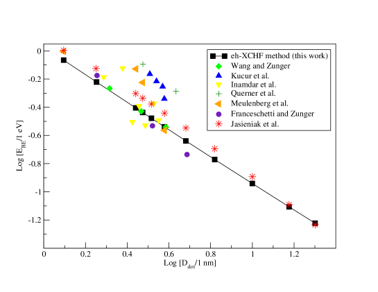
Figure 1: Log of binding energy ($E_{BE}$) versus log of diameter for CdSe quantum dots. The values from the eh-XCHF calculations are compared with results from earlier studies by Wang et al. Wang and Zunger (1996), Franceschetti et al. Meulenberg et al. (2009), Meulenberg et al. Franceschetti and Zunger (1997), Jasieniak et al. Jasieniak et al. (2011), Kucur et al. Kucur et al. (2003), Inamdar et al. Inamdar et al. (2008), and Querner et al. Querner et al. (2005) The details of the comparison are presented in the text.

For $D_{\mathrm{dot}}$ equal to $1.8$, $3.32$ and $4.82\,\mathrm{nm}$, Franceschetti and Zunger have computed binding energies using atomistic pseudopotential based configuration interaction method Franceschetti and Zunger (1997) and the exciton binding energies shown in Figure 1 were obtained from the tabulated values in Ref. 32. In a recent combined experimental and theoretical investigation, Jasieniak et al. Jasieniak et al. (2011) have reported size-dependent valence and conduction band energies of CdSe quantum dots. The values from the Jasieniak et al. studies in Figure 1 were obtained from the least-square fit equation provided in Ref. 34. The remaining data points were obtained from the plot in Ref. 34. The log-log plot in Figure 1 shows that the computed binding energy is described very well by a linear-fit and the exciton binding energy scales as $D^{-n}$ with respect to the dot size. This observation is consistent with trend observed in earlier studies. Franceschetti and Zunger (1997); Meulenberg et al. (2009); Jasieniak et al. (2011) We find that the exciton binding energy from the eh-XCHF calculations are in very good agreement with the atomistic pseudopotential calculations by Wang et al. Wang and Zunger (1996) and Franceschetti et al. Franceschetti and Zunger (1997) Comparing between eh-XCHF and Jasieniak et al. Jasieniak et al. (2011) results show that the eh-XCHF values are lower than the Jasieniak et al. values for small dot sizes, but the difference becomes smaller with increasing dot size. One possible explanations for this observation is that the smaller quantum dots have high surface to volume ratios and their optical properties are dominated by surface effects Jasieniak and Mulvaney (2007); Luther and Pietryga (2013) that are not currently included in the eh-XCHF calculations. The plot in Figure 1 highlights the ability of the eh-XCHF method to predict exciton binding energies for large quantum dots.

IV.2 Electron-hole Coulomb energy

Another important quantity that is directly related to the electron-hole interaction is the electron-hole Coulomb energy. We have used the definition given by Franceschetti and Zunger Franceschetti and Zunger (1997) and calculated the electron-hole Coulomb energy using the following expression

$$A =\int d\mathbf{r}_{\mathrm{e}}d\mathbf{r}_{\mathrm{h}}\,\,\rho_{\mathrm{eh}}(\mathbf{r}_{\mathrm{e}},\mathbf{r}_{\mathrm{h}})r^{-1}_{\mathrm{eh}}.$$ (19)

In Figure 2, we have compared the electron-hole Coulomb energy with the pseudopotential+CI calculations by Franceschetti and Zunger and the results were found to be in good agreement with each other.

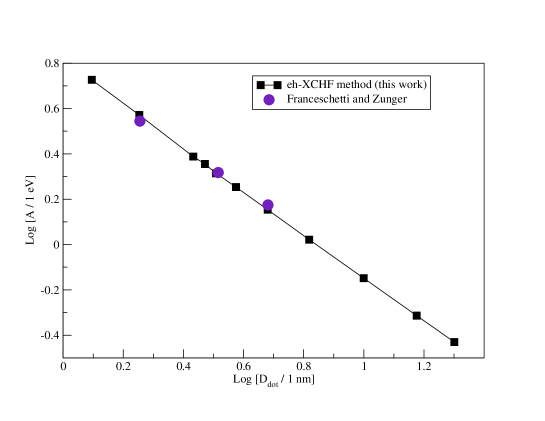
Figure 2: Log of Coulomb energy ($A$) for CdSe quantum dots versus log of diameter of quantum dot.

If the dielectric function is approximated by a constant, then the exciton binding energy is related to Coulomb energy by the expression

$$E_{\mathrm{BE}}=\epsilon^{-1}A\quad\mathrm{for}\quad\epsilon(\mathbf{r}^{\mathrm{e}},\mathbf{r}^{\mathrm{h}})=\epsilon.$$ (20)

The Coulomb energy is a very important quantity because it allows us to directly compare the quality of electron-hole pair density without introducing any additional approximation due to the choice of the dielectric function used for computation of the binding energy. The good agreement between the two methods provides important verification of the implementation of the eh-XCHF method.

IV.3 Recombination probability

In addition to exciton binding energies, electron-hole recombination probabilities were also calculated. Using the expression in Eq. (4), the electron-hole pair density from the eh-XCHF method was used in the computation of electron-hole recombination probabilities and the results are presented in Figure 3.

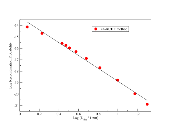
Figure 3: Log of recombination probability ($\mathrm{P_{eh}}$) of CdSe quantum dots versus log of diameter of quantum dot.

A log-log plot of $P_{\mathrm{eh}}$ versus $D_{\mathrm{dot}}$ indicates that the recombination probability also follows $D_{\mathrm{dot}}^{-n}$ dependence with dot diameter. One of the key results from this study is that the electron-hole recombination probability decreases at a much faster rate that the exciton-binding energy with increasing dot size. This is illustrated in Figure 4,

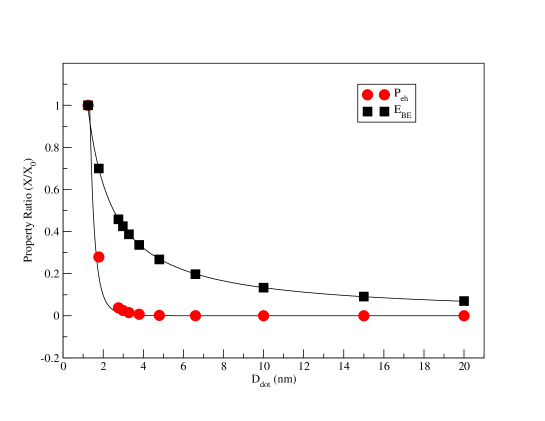
Figure 4: Comparison of $E_{\mathrm{BE}}$ and $P_{\mathrm{eh}}$ relative properties versus $r_{\mathrm{dot}}$.

where comparison of the relative binding energy and recombination probability is presented with respect to dot size. It was found that for a factor of 16.1 change in the dot diameter, the exciton binding energy and the recombination probability decrease by a factor of $14.4$ and $5.5\times 10^{6}$, respectively. The linear regression equations of the Coulomb energy, exciton binding energy and electron-hole recombination probability as function of dot diameter are summarized in Table 5.

Table 5: Linear regression equation of Coulomb energy, exciton binding energy, and electron-hole recombination probability with respect to dot diameter

Property	Equation
$\mathrm{log}[\mathrm{A}/\mathrm{eV}]$	$-0.958\,\mathrm{log[D/\mathrm{nm}}]+0.8106$
$\mathrm{log}[\mathrm{E}_{\mathrm{{BE}}}/\mathrm{eV}]$	$-0.958\,\mathrm{log[D/\mathrm{nm}}]+0.0182$
$\mathrm{log}\mathrm{P}_{\mathrm{{eh}}}$	$-5.590\,\mathrm{log[D/nm}]-13.271$

It is seen that the slope for the recombination is substantially higher than the binding energy.

V Conclusions

In conclusion, we have presented a multifaceted study of effect of dot size on electron-hole interaction in CdSe quantum dots. The electron-hole explicitly correlated Hartree-Fock method was used for computation of exciton binding energy and electron-hole recombination probability. It was found that both exciton binding energy and electron-hole recombination probability decreases with increasing dot size and both quantities scale as $D_{\mathrm{dot}}^{-n}$ with respect to the diameter of the quantum dot. The computed exciton binding energies were found to be in good agreement with previously reported results. One of significant results from these calculations is that that the electron-hole recombination probability decreases at a substantially higher rate than the binding energy with increasing dot size. Changing the dot size by a factor of 14 resulted in a decrease in the electron-hole recombination probability by a factor of $10^{6}$. We believe this to be a significant result that can enhance our understanding of the electron-hole interaction in quantum dots.

References

- Zhu and Lian (2012) Haiming Zhu and Tianquan Lian, “Enhanced multiple exciton dissociation from cdse quantum rods: The effect of nanocrystal shape,” Journal of the American Chemical Society 134, 11289–11297 (2012).
- Ghosh et al. (2012) Yagnaseni Ghosh, Benjamin D. Mangum, Joanna L. Casson, Darrick J. Williams, Han Htoon, and Jennifer A. Hollingsworth, “New insights into the complexities of shell growth and the strong influence of particle volume in nonblinking “giant” core/shell nanocrystal quantum dots,” Journal of the American Chemical Society 134, 9634–9643 (2012).
- Bae et al. (2013) Wan Ki Bae, Lazaro A. Padilha, Young-Shin Park, Hunter McDaniel, Istvan Robel, Jeffrey M. Pietryga, and Victor I. Klimov, “Controlled alloying of the core-shell interface in cdse/cds quantum dots for suppression of auger recombination,” ACS Nano 7, 3411–3419 (2013).
- Lin et al. (2011) Zhibin Lin, Alberto Franceschetti, and Mark T. Lusk, “Size dependence of the multiple exciton generation rate in cdse quantum dots,” ACS Nano 5, 2503–2511 (2011).
- Alam et al. (2012) Rabeka Alam, Danielle M. Fontaine, Bruce R. Branchini, and Mathew M. Maye, “Designing quantum rods for optimized energy transfer with firefly luciferase enzymes,” Nano Letters 12, 3251–3256 (2012).
- Han et al. (2010) Hyunjoo Han, Gianna Di Francesco, and Mathew M. Maye, “Size control and photophysical properties of quantum dots prepared via a novel tunable hydrothermal route,” The Journal of Physical Chemistry C 114, 19270–19277 (2010).
- Williams et al. (2013) B L Williams, D P Halliday, B G Mendis, and K Durose, “Microstructure and point defects in cdte nanowires for photovoltaic applications,” Nanotechnology 24, 135703 (2013).
- Yin et al. (2013) Jun Yin, Chuang Yue, Yashu Zang, Ching-Hsueh Chiu, Jinchai Li, Hao-Chung Kuo, Zhihao Wu, Jing Li, Yanyan Fang, and Changqing Chen, “Effect of the surface-plasmon-exciton coupling and charge transfer process on the photoluminescence of metal-semiconductor nanostructures,” Nanoscale 5, 4436–4442 (2013).
- Jaeger et al. (2012) Heather M. Jaeger, Sean Fischer, and Oleg V. Prezhdo, “The role of surface defects in multi-exciton generation of lead selenide and silicon semiconductor quantum dots,” The Journal of Chemical Physics 136, 064701 (2012).
- Kilina et al. (2012) Svetlana Kilina, Kirill A. Velizhanin, Sergei Ivanov, Oleg V. Prezhdo, and Sergei Tretiak, “Surface ligands increase photoexcitation relaxation rates in cdse quantum dots,” ACS Nano 6, 6515–6524 (2012).
- Kilina et al. (2009a) Svetlana Kilina, Sergei Ivanov, and Sergei Tretiak, “Effect of surface ligands on optical and electronic spectra of semiconductor nanoclusters,” Journal of the American Chemical Society 131, 7717–7726 (2009a).
- Kilina et al. (2009b) Svetlana V. Kilina, Dmitri S. Kilin, and Oleg V. Prezhdo, “Breaking the phonon bottleneck in pbse and cdse quantum dots: Time-domain density functional theory of charge carrier relaxation,” ACS Nano 3, 93–99 (2009b).
- Kelley (2010) A.M. Kelley, “Electron-phonon coupling in cdse nanocrystals,” Journal of Physical Chemistry Letters 1, 1296–1300 (2010).
- Kelley (2011) A.M. Kelley, “Electron-phonon coupling in cdse nanocrystals from an atomistic phonon model,” ACS Nano 5, 5254–5262 (2011).
- Kelley et al. (2012) A.M. Kelley, Q. Dai, Z.-j. Jiang, J.A. Baker, and D.F. Kelley, “Resonance raman spectra of wurtzite and zincblende cdse nanocrystals,” Chemical Physics (2012), 10.1016/j.chemphys.2012.09.029.
- Kilina et al. (2011) S.V. Kilina, D.S. Kilin, V.V. Prezhdo, and O.V. Prezhdo, “Theoretical study of electron-phonon relaxation in pbse and cdse quantum dots: Evidence for phonon memory,” Journal of Physical Chemistry C 115, 21641–21651 (2011).
- Hyeon-Deuk and Prezhdo (2011) K. Hyeon-Deuk and O.V. Prezhdo, “Time-domain ab initio study of auger and phonon-assisted auger processes in a semiconductor quantum dot,” Nano Letters 11, 1845–1850 (2011).
- Hyeon-Deuk and Prezhdo (2012a) K. Hyeon-Deuk and O.V. Prezhdo, “Photoexcited electron and hole dynamics in semiconductor quantum dots: Phonon-induced relaxation, dephasing, multiple exciton generation and recombination,” Journal of Physics Condensed Matter 24 (2012a), 10.1088/0953-8984/24/36/363201.
- Kilina et al. (2013) S.V. Kilina, A.J. Neukirch, B.F. Habenicht, D.S. Kilin, and O.V. Prezhdo, “Quantum zeno effect rationalizes the phonon bottleneck in semiconductor quantum dots,” Physical Review Letters 110 (2013), 10.1103/PhysRevLett.110.180404.
- Musa et al. (2011) I. Musa, F. Massuyeau, L. Cario, J. L. Duvail, S. Jobic, P. Deniard, and E. Faulques, “Temperature and size dependence of time-resolved exciton recombination in zno quantum dots,” Applied Physics Letters 99, 243107 (2011).
- Chon et al. (2011) Bonghwan Chon, Jiwon Bang, Juwon Park, Cherlhyun Jeong, Jong Hwa Choi, Jong-Bong Lee, Taiha Joo, and Sungjee Kim, “Unique temperature dependence and blinking behavior of cdte/cdse (core/shell) type-ii quantum dots,” The Journal of Physical Chemistry C 115, 436–442 (2011).
- Franceschetti and Zunger (2001) Alberto Franceschetti and Alex Zunger, “Exciton dissociation and interdot transport in cdse quantum-dot molecules,” Phys. Rev. B 63, 153304 (2001).
- Zhu et al. (2011) Haiming Zhu, Nianhui Song, and Tianquan Lian, “Wave function engineering for ultrafast charge separation and slow charge recombination in type ii core/shell quantum dots,” Journal of the American Chemical Society 133, 8762–8771 (2011).
- Zhu et al. (2010) Haiming Zhu, Nianhui Song, and Tianquan Lian, “Controlling charge separation and recombination rates in cdse/zns type i core-shell quantum dots by shell thicknesses,” Journal of the American Chemical Society 132, 15038–15045 (2010).
- Hoy et al. (0) Jessica Hoy, Paul J. Morrison, Lindsey K. Steinberg, William E. Buhro, and Richard A. Loomis, “Excitation energy dependence of the photoluminescence quantum yields of core and core/shell quantum dots,” The Journal of Physical Chemistry Letters 0, 2053–2060 (0).
- Li et al. (2012) Dehui Li, Jun Zhang, Qing Zhang, and Qihua Xiong, “Electric-field-dependent photoconductivity in cds nanowires and nanobelts: Exciton ionization, franz-keldysh, and stark effects,” Nano Letters 12, 2993–2999 (2012).
- Yaacobi-Gross et al. (2011) Nir Yaacobi-Gross, Michal Soreni-Harari, Marina Zimin, Shifi Kababya, Asher Schmidt, and Nir Tessler, “Molecular control of quantum-dot internal electric field and its application to cdse-based solar cells,” Nature Materials 10, 974–979 (2011).
- Liu et al. (2012) Su Liu, Nicholas J. Borys, Jing Huang, Dmitri V. Talapin, and John M. Lupton, “Exciton storage in cdse/cds tetrapod semiconductor nanocrystals: Electric field effects on exciton and multiexciton states,” Phys. Rev. B 86, 045303 (2012).
- Perebeinos and Avouris (2007) Vasili Perebeinos and Phaedon Avouris, “Exciton ionization, franz-keldysh, and stark effects in carbon nanotubes,” Nano Letters 7, 609–613 (2007).
- Blanton et al. (2013) Christopher J. Blanton, Christopher Brenon, and Arindam Chakraborty, “Development of polaron-transformed explicitly correlated full configuration interaction method for investigation of quantum-confined stark effect in gaas quantum dots,” The Journal of Chemical Physics 138, 054114 (2013).
- Park et al. (2012) KyoungWon Park, Zvicka Deutsch, J. Jack Li, Dan Oron, and Shimon Weiss, “Single molecule quantum-confined stark effect measurements of semiconductor nanoparticles at room temperature,” ACS Nano 6, 10013–10023 (2012).
- Franceschetti and Zunger (1997) Alberto Franceschetti and Alex Zunger, “Direct pseudopotential calculation of exciton coulomb and exchange energies in semiconductor quantum dots,” Phys. Rev. Lett. 78, 915–918 (1997).
- Meulenberg et al. (2009) Robert W. Meulenberg, Jonathan R.I. Lee, Abraham Wolcott, Jin Z. Zhang, Louis J. Terminello, and Tony van Buuren, “Determination of the exciton binding energy in cdse quantum dots,” ACS Nano 3, 325–330 (2009).
- Jasieniak et al. (2011) Jacek Jasieniak, Marco Califano, and Scott E. Watkins, “Size-dependent valence and conduction band-edge energies of semiconductor nanocrystals,” ACS Nano 5, 5888–5902 (2011).
- Maan et al. (1984) J. C. Maan, G. Belle, A. Fasolino, M. Altarelli, and K. Ploog, “Magneto-optical determination of exciton binding energy in gaas- quantum wells,” Phys. Rev. B 30, 2253–2256 (1984).
- Ramvall et al. (1998) Peter Ramvall, Satoru Tanaka, Shintaro Nomura, Philippe Riblet, and Yoshinobu Aoyagi, “Observation of confinement-dependent exciton binding energy of gan quantum dots,” Applied Physics Letters 73, 1104–1106 (1998).
- Wang and Zunger (1996) Lin-Wang Wang and Alex Zunger, “Pseudopotential calculations of nanoscale cdse quantum dots,” Phys. Rev. B 53, 9579–9582 (1996).
- Kucur et al. (2003) Erol Kucur, Jurgen Riegler, Gerald A. Urban, and Thomas Nann, “Determination of quantum confinement in cdse nanocrystals by cyclic voltammetry,” The Journal of Chemical Physics 119, 2333–2337 (2003).
- Inamdar et al. (2008) Shaukatali N. Inamdar, Pravin P. Ingole, and Santosh K. Haram, “Determination of band structure parameters and the quasi-particle gap of cdse quantum dots by cyclic voltammetry,” ChemPhysChem 9, 2574–2579 (2008).
- Querner et al. (2005) Claudia Querner, Peter Reiss, Said Sadki, Malgorzata Zagorska, and Adam Pron, “Size and ligand effects on the electrochemical and spectroelectrochemical responses of cdse nanocrystals,” Phys. Chem. Chem. Phys. 7, 3204–3209 (2005).
- García-Santamaría et al. (2009) Florencio García-Santamaría, Yongfen Chen, Javier Vela, Richard D. Schaller, Jennifer A. Hollingsworth, and Victor I. Klimov, “Suppressed auger recombination in “giant” nanocrystals boosts optical gain performance,” Nano Letters 9, 3482–3488 (2009).
- Wang et al. (2003) Lin-Wang Wang, Marco Califano, Alex Zunger, and Alberto Franceschetti, “Pseudopotential theory of auger processes in cdse quantum dots,” Phys. Rev. Lett. 91, 056404 (2003).
- Hyeon-Deuk and Prezhdo (2012b) Kim Hyeon-Deuk and Oleg V. Prezhdo, “Multiple exciton generation and recombination dynamics in small si and cdse quantum dots: An ab initio time-domain study,” ACS Nano 6, 1239–1250 (2012b).
- Rabani and Baer (2010) Eran Rabani and Roi Baer, “Theory of multiexciton generation in semiconductor nanocrystals,” Chemical Physics Letters 496, 227 – 235 (2010).
- Jaeger et al. (Article ASAP) Heather M. Jaeger, Kim Hyeon-Deuk, and Oleg V. Prezhdo, “Exciton multiplication from first principles,” Accounts of Chemical Research (Article ASAP), 10.1021/ar3002365.
- Vela et al. (2010) Javier Vela, Han Htoon, Yongfen Chen, Young-Shin Park, Yagnaseni Ghosh, Peter M. Goodwin, James H. Werner, Nathan P. Wells, Joanna L. Casson, and Jennifer A. Hollingsworth, “Effect of shell thickness and composition on blinking suppression and the blinking mechanism in “giant” cdse/cds nanocrystal quantum dots,” Journal of Biophotonics 3, 706–717 (2010).
- Rawalekar et al. (2010) Sachin Rawalekar, Sreejith Kaniyankandy, Sandeep Verma, and Hirendra N. Ghosh, “Ultrafast charge carrier relaxation and charge transfer dynamics of cdte/cds core-shell quantum dots as studied by femtosecond transient absorption spectroscopy,” The Journal of Physical Chemistry C 114, 1460–1466 (2010).
- Nemchinov et al. (2008) Alexander Nemchinov, Maria Kirsanova, Nishshanka N. Hewa-Kasakarage, and Mikhail Zamkov, “Synthesis and characterization of type ii znse/cds core/shell nanocrystals,” The Journal of Physical Chemistry C 112, 9301–9307 (2008).
- Yan et al. (2011) Yueran Yan, Gang Chen, and P. Gregory Van Patten, “Ultrafast exciton dynamics in cdte nanocrystals and core/shell cdte/cds nanocrystals,” The Journal of Physical Chemistry C 115, 22717–22728 (2011).
- Xu et al. (2012) Zhihua Xu, Corey R. Hine, Mathew M. Maye, Qingping Meng, and Mircea Cotlet, “Shell thickness dependent photoinduced hole transfer in hybrid conjugated polymer/quantum dot nanocomposites: From ensemble to single hybrid level,” ACS Nano 6, 4984–4992 (2012).
- Noguchi et al. (2012) Y. Noguchi, O. Sugino, M. Nagaoka, S. Ishii, and K. Ohno, “A gwbethe-salpeter calculation on photoabsorption spectra of (cdse) 3 and (cdse) 6 clusters,” Journal of Chemical Physics 137, 024306 (2012).
- Lopez Del Puerto et al. (2008) M. Lopez Del Puerto, M.L. Tiago, and J.R. Chelikowsky, “Ab initio methods for the optical properties of cdse clusters,” Physical Review B - Condensed Matter and Materials Physics 77, 045404 (2008).
- Del Puerto et al. (2006) M.L. Del Puerto, M.L. Tiago, and J.R. Chelikowsky, “Excitonic effects and optical properties of passivated cdse clusters,” Physical Review Letters 97, 096401 (2006).
- Nguyen et al. (2010) K.A. Nguyen, P.N. Day, and Pachte, “Understanding structural and optical properties of nanoscale cdse magic-size quantum dots: Insight from computational prediction,” Journal of Physical Chemistry C 114, 16197–16209 (2010).
- Yang et al. (2011) P. Yang, S. Tretiak, and S. Ivanov, “Influence of surfactants and charges on cdse quantum dots,” Journal of Cluster Science 22, 405–431 (2011).
- Albert et al. (2011) V.V. Albert, S.A. Ivanov, S. Tretiak, and S.V. Kilina, “Electronic structure of ligated cdse clusters: Dependence on dft methodology,” Journal of Physical Chemistry C 115, 15793–15800 (2011).
- Kilin et al. (2007) D.S. Kilin, K. Tsemekhman, O.V. Prezhdo, E.I. Zenkevich, and C. von Borczyskowski, “Ab initio study of exciton transfer dynamics from a core-shell semiconductor quantum dot to a porphyrin-sensitizer,” Journal of Photochemistry and Photobiology A: Chemistry 190, 342–351 (2007).
- Liu et al. (2009) C. Liu, S.-Y. Chung, S. Lee, S. Weiss, and D. Neuhauser, “Adsorbate-induced absorption redshift in an organic-inorganic cluster conjugate: Electronic effects of surfactants and organic adsorbates on the lowest excited states of a methanethiol-cdse conjugate,” Journal of Chemical Physics 131 (2009), 10.1063/1.3251774.
- Chung et al. (2009) S.-Y. Chung, S. Lee, C. Liu, and D. Neuhauser, “Structures and electronic spectra of cdse-cys complexes: Density functional theory study of a simple peptide-coated nanocluster,” Journal of Physical Chemistry B 113, 292–301 (2009).
- Kim et al. (2010) H.S. Kim, S.-W. Jang, S.Y. Chung, S. Lee, Y. Lee, B. Kim, C. Liu, and D. Neuhauser, “Effects of bioconjugation on the structures and electronic spectra of cdse: Density functional theory study of cdse - adenine complexes,” Journal of Physical Chemistry B 114, 471–479 (2010).
- Nadler and Sanz (2013) R. Nadler and J.F. Sanz, “Simulating the optical properties of cdse clusters using the rt-tddft approach,” Theoretical Chemistry Accounts 132, 1–9 (2013).
- Abuelela et al. (2012) A.M. Abuelela, T.A. Mohamed, and O.V. Prezhdo, “Dft simulation and vibrational analysis of the ir and raman spectra of a cdse quantum dot capped by methylamine and trimethylphosphine oxide ligands,” Journal of Physical Chemistry C 116, 14674–14681 (2012).
- Fischer et al. (2012) S.A. Fischer, A.M. Crotty, S.V. Kilina, S.A. Ivanov, and S. Tretiak, “Passivating ligand and solvent contributions to the electronic properties of semiconductor nanocrystals,” Nanoscale 4, 904–914 (2012).
- Del Ben et al. (2011) M. Del Ben, R.W.A. Havenith, R. Broer, and M. Stener, “Density functional study on the morphology and photoabsorption of cdse nanoclusters,” Journal of Physical Chemistry C 115, 16782–16796 (2011).
- Turkowski et al. (2009) V. Turkowski, A. Leonardo, and C.A. Ullrich, “Time-dependent density-functional approach for exciton binding energies,” Physical Review B - Condensed Matter and Materials Physics 79 (2009), 10.1103/PhysRevB.79.233201.
- Li and Ullrich (2011) Y. Li and C.A. Ullrich, “Time-dependent transition density matrix,” Chemical Physics 391, 157–163 (2011).
- Yang et al. (2012) Z.-H. Yang, Y. Li, and C.A. Ullrich, “A minimal model for excitons within time-dependent density-functional theory,” Journal of Chemical Physics 137 (2012), 10.1063/1.4730031.
- Yang and Ullrich (2013) Z.-H. Yang and C.A. Ullrich, “Direct calculation of exciton binding energies with time-dependent density-functional theory,” Physical Review B - Condensed Matter and Materials Physics 87 (2013), 10.1103/PhysRevB.87.195204.
- Neuhauser et al. (2013) D. Neuhauser, E. Rabani, and R. Baer, “Expeditious stochastic calculation of random-phase approximation energies for thousands of electrons in three dimensions,” Journal of Physical Chemistry Letters 4, 1172–1176 (2013).
- Franceschetti et al. (1999) A. Franceschetti, H. Fu, L. W. Wang, and A. Zunger, “Many-body pseudopotential theory of excitons in inp and cdse quantum dots,” Phys. Rev. B 60, 1819–1829 (1999).
- Baer and Rabani (2013) Roi Baer and Eran Rabani, “Communication: Biexciton generation rates in cdse nanorods are length independent,” The Journal of Chemical Physics 138, 051102 (2013).
- Rabani et al. (1999) Eran Rabani, Balazs Hetenyi, B. J. Berne, and L. E. Brus, “Electronic properties of cdse nanocrystals in the absence and presence of a dielectric medium,” The Journal of Chemical Physics 110, 5355–5369 (1999).
- Wang and Zunger (1994) L.-W. Wang and A. Zunger, “Solving schrödinger’s equation around a desired energy: Application to silicon quantum dots,” The Journal of Chemical Physics 100, 2394–2397 (1994).
- Canning et al. (2000) A. Canning, L.W. Wang, A. Williamson, and A. Zunger, “Parallel empirical pseudopotential electronic structure calculations for million atom systems,” Journal of Computational Physics 160, 29–41 (2000).
- Toledo and Rabani (2002) S. Toledo and E. Rabani, “Very large electronic structure calculations using an out-of-core filter-diagonalization method,” Journal of Computational Physics 180, 256–269 (2002).
- Vömel et al. (2008) C. Vömel, S.Z. Tomov, O.A. Marques, A. Canning, L.-W. Wang, and J.J. Dongarra, “State-of-the-art eigensolvers for electronic structure calculations of large scale nano-systems,” Journal of Computational Physics 227, 7113–7124 (2008).
- Jordan et al. (2012) G. Jordan, M. Marsman, Y.-S. Kim, and G. Kresse, “Fast iterative interior eigensolver for millions of atoms,” Journal of Computational Physics 231, 4836–4847 (2012).
- Mazziotti (2007) D.A. Mazziotti, Advances in Chemical Physics, Reduced-Density-Matrix Mechanics: With Application to Many-Electron Atoms and Molecules, Advances in Chemical Physics (Wiley, 2007).
- Elward et al. (2012a) Jennifer M. Elward, Barbara Thallinger, and Arindam Chakraborty, “Calculation of electron-hole recombination probability using explicitly correlated hartree-fock method,” The Journal of Chemical Physics 136, 124105 (2012a).
- Elward et al. (2012b) Jennifer M. Elward, Jacob Hoffman, and Arindam Chakraborty, “Investigation of electron-hole correlation using explicitly correlated configuration interaction method,” Chemical Physics Letters 535, 182 – 186 (2012b).
- Wimmer et al. (2006a) M. Wimmer, S. V. Nair, and J. Shumway, “Biexciton recombination rates in self-assembled quantum dots,” Physical Review B - Condensed Matter and Materials Physics 73, 1–10 (2006a).
- Cancio and Chang (1990) A.C. Cancio and Y.-C. Chang, “Quantum monte carlo study of polyexcitons in semiconductors,” Physical Review B 42, 11317–11324 (1990).
- Cancio and Chang (1993) A.C. Cancio and Y.-C. Chang, “Quantum monte carlo studies of binding energy and radiative lifetime of bound excitons in direct-gap semiconductors,” Physical Review B 47, 13246–13259 (1993).
- Zhu et al. (1996) Xuejun Zhu, Mark S. Hybertsen, and P. B. Littlewood, “Electron-hole system revisited: A variational quantum monte carlo study,” Phys. Rev. B 54, 13575–13580 (1996).
- Boys (1960) S. F. Boys, “The integral formulae for the variational solution of the molecular many-electron wave equations in terms of gaussian functions with direct electronic correlation,” Proceedings of the Royal Society of London. Series A. Mathematical and Physical Sciences 258, 402–411 (1960).
- Persson and Taylor (1996) B. Joakim Persson and Peter R. Taylor, “Accurate quantum-chemical calculations: The use of gaussian-type geminal functions in the treatment of electron correlation,” The Journal of Chemical Physics 105, 5915–5926 (1996).
- Hu et al. (1990) Y. Z. Hu, M. Lindberg, and S. W. Koch, “Theory of optically excited intrinsic semiconductor quantum dots,” Phys. Rev. B 42, 1713–1723 (1990).
- Burovski et al. (2001) E. A. Burovski, A. S. Mishchenko, N. V. Prokofév, and B. V. Svistunov, “Diagrammatic quantum monte carlo for two-body problems: Applied to excitons,” Phys. Rev. Lett. 87, 186402 (2001).
- Wimmer et al. (2006b) Michael Wimmer, S. V. Nair, and J. Shumway, “Biexciton recombination rates in self-assembled quantum dots,” Phys. Rev. B 73, 165305 (2006b).
- Woggon (1997) U. Woggon, Springer Tracts in Modern Physics, Springer Tracts in Modern Physics No. v. 136 (Springer-Verlag., 1997).
- Braskén et al. (2001) M. Braskén, M. Lindberg, D. Sundholm, and J. Olsen, “Full configuration interaction calculations of electron-hole correlation effects in strain-induced quantum dots,” Physica Status Solidi (B) Basic Research 224, 775–779 (2001).
- Corni et al. (2003a) S. Corni, M. Braskén, M. Lindberg, J. Olsen, and D. Sundholm, “Stabilization energies of charged multiexciton complexes calculated at configuration interaction level,” Physica E: Low-Dimensional Systems and Nanostructures 18, 436–442 (2003a).
- Corni et al. (2003b) S. Corni, M. Braskén, M. Lindberg, J. Olsen, and D. Sundholm, “Electron-hole recombination density matrices obtained from large configuration-interaction expansions,” Physical Review B - Condensed Matter and Materials Physics 67, 853141–853147 (2003b).
- Corni et al. (2003c) S. Corni, M. Braskén, M. Lindberg, J. Olsen, and D. Sundholm, “Size dependence of the electron-hole recombination rates in semiconductor quantum dots,” Physical Review B - Condensed Matter and Materials Physics 67, 453131–453139 (2003c).
- Vänskä et al. (2006) T. Vänskä, M. Lindberg, J. Olsen, and D. Sundholm, “Computational methods for studies of multiexciton complexes,” Physica Status Solidi (B) Basic Research 243, 4035–4045 (2006).
- Vänskä and Sundholm (2010) T. Vänskä and D. Sundholm, “Interpretation of the photoluminescence spectrum of double quantum rings,” Physical Review B - Condensed Matter and Materials Physics 82 (2010), 10.1103/PhysRevB.82.085306.
- Sundholm and Vänskä (2012) D. Sundholm and T. Vänskä, “Computational methods for studies of semiconductor quantum dots and rings,” Annual Reports on the Progress of Chemistry - Section C 108, 96–125 (2012).
- (98) Jennifer M. Elward and Arindam Chakraborty, “Atomistic pseudopotential calculation on cdse quantum dots using electron-hole explicitly correlated hartree-fock method,” (to be submitted) .
- Halonen et al. (1992) V. Halonen, T. Chakraborty, and P. Pietiläinen, “Excitons in a parabolic quantum dot in magnetic fields,” Physical Review B 45, 5980–5985 (1992).
- El-Said (1994) Mohammad El-Said, “Ground-state energy of an exciton in a parabolic quantum dot,” Semiconductor Science and Technology 9, 272–274 (1994).
- Jaziri and Bennaceur (1994) S. Jaziri and R. Bennaceur, “Excitons in parabolic quantum dots in electric and magnetic fields,” Semiconductor Science and Technology 9, 1775–1780 (1994).
- Lamouche and Fishman (1998) G. Lamouche and G. Fishman, “Two interacting electrons in a three-dimensional parabolic quantum dot: A simple solution,” Journal of Physics Condensed Matter 10, 7857–7867 (1998).
- Xie and Gu (2003) W. Xie and J. Gu, “Exciton bound to a neutral donor in parabolic quantum dots,” Physics Letters, Section A: General, Atomic and Solid State Physics 312, 385–390 (2003).
- Xie (2005) W. Xie, “Exciton states trapped by a parabolic quantum dot,” Physica B: Condensed Matter 358, 109–113 (2005).
- Xie (2009) W. Xie, “Effect of an electric field and nonlinear optical rectification of confined excitons in quantum dots,” Physica Status Solidi (B) Basic Research 246, 2257–2262 (2009).
- Karimi and Rezaei (2011) M.J. Karimi and G. Rezaei, “Effects of external electric and magnetic fields on the linear and nonlinear intersubband optical properties of finite semi-parabolic quantum dots,” Physica B: Condensed Matter 406, 4423 – 4428 (2011).
- Nammas et al. (2011) F.S. Nammas, A.S. Sandouqa, H.B. Ghassib, and M.K. Al-Sugheir, “Thermodynamic properties of two-dimensional few-electrons quantum dot using the static fluctuation approximation (sfa),” Physica B: Condensed Matter 406, 4671 – 4677 (2011).
- Rezaei et al. (2011) G. Rezaei, B. Vaseghi, and M. Sadri, “External electric field effect on the optical rectification coefficient of an exciton in a spherical parabolic quantum dot,” Physica B: Condensed Matter 406, 4596 – 4599 (2011).
- Elward et al. (2012c) Jennifer M. Elward, Johannes Hoja, and Arindam Chakraborty, “Variational solution of the congruently transformed hamiltonian for many-electron systems using a full-configuration-interaction calculation,” Phys. Rev. A 86, 062504 (2012c).
- (110) Mike Bayne, John Drogo, and Arindam Chakraborty, “Infinite-order diagrammatic summation approach to explicitly correlated congruent transformed hamiltonian,” (to be submitted) .
- Swalina et al. (2006) Chet Swalina, Michael V. Pak, Arindam Chakraborty, and Sharon Hammes-Schiffer, “Explicit dynamical electron-proton correlation in the nuclear-electronic orbital framework,” The Journal of Physical Chemistry A 110, 9983–9987 (2006).
- Jasieniak and Mulvaney (2007) Jacek Jasieniak and Paul Mulvaney, “From cd-rich to se-rich-the manipulation of cdse nanocrystal surface stoichiometry,” Journal of the American Chemical Society 129, 2841–2848 (2007).
- Luther and Pietryga (2013) Joseph M Luther and Jeffrey M Pietryga, “Stoichiometry control in quantum dots: A viable analog to impurity doping of bulk materials,” ACS nano 7, 1845–1849 (2013).