Asymptotic Analysis and Random Sampling of Digitally Convex Polyominoes

Abstract

Recent work of Brlek et al. gives a characterization of digitally convex polyominoes using combinatorics on words. From this work, we derive a combinatorial symbolic description of digitally convex polyominoes and use it to analyze their limit properties and build a uniform sampler. Experimentally, our sampler shows a limit shape for large digitally convex polyominoes.

Introduction

In discrete geometry, a finite set of unit square cells is said to be a digitally convex polyomino if it is exactly the set of unit cells included in a convex region of the plane. We only consider digitally convex polyominoes up to translation. The perimeter of a digitally convex polyomino is that of the smallest rectangular box that contains it.

The notion of digitally convex polyominoes arises naturally in the context of curvature estimators and consequently in the important field of pattern recognition [18, 10].

Brlek et al. [9] described a characterization of digitally convex polyominoes, in terms of words coding their contour. In this paper, we reformulate this characterization in the context of constructible combinatorial classes and we use it to build and analyze an algorithm to randomly sample digitally convex polyominoes.

Our algorithm, based on a model of parametrized samplers, called Boltzmann samplers [11], draws digitally convex polyominoes at random. Although all possible digitally convex polyominoes have positive probability, the perimeter of the randomly generated polyomino being itself random, two different structures with the same perimeter appear with the same probability. Moreover, an appropriate choice of the tuning parameter allows the user to adjust the random model, typically in order to generate large structures. We present also in this paper how to tune this parameter.

The Boltzmann model of random sampling, as introduced in [11], is a general method for the random generation of discrete combinatorial structures where, for some real parameter $x>0$, each possible structure $\gamma$, with (integer) size $|\gamma|$, is obtained with probability proportional to $x^{|\gamma|}$. A Boltzmann sampler for a combinatorial class $\mathcal{C}$ is a randomized algorithm that takes as input a parameter $x$, and outputs a random element of $\mathcal{C}$ according to the Boltzmann distribution with parameter $x$.

Samples obtained via this generator suggested that large random quarters of digitally convex polyominoes exhibit a limit shape. We identify and prove this limit shape in Section 2

The first section is dedicated to introducing the characterization of Brlek et al [9] in the framework of symbolic methods. In Section 2, we analyze asymptotic properties of quarters of digitally convex polyominoes. Finally, we give in Section 3 the samplers for digitally convex polyominoes and some analysis for the complexity of the sampling.

1 Characterization of digitally convex polygons

The goal of this section is to recall (without proofs) the characterization by Brlek, Lachaud, Provençal, Reutenauer [9] of digitally convex polyominoes and recast it in terms of the symbolic method. This characterization is the starting point to efficiently sample large digitally convex polyominoes, and is thus needed in the next chapters.

1.1 Digitally convex polyominoes

Definition 1.1.

A digitally convex polyomino, DCP for short, is the set of all cells of $\mathbb{Z}^{2}$ included in a bounded convex region of the plane.

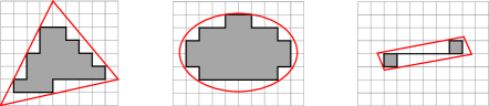
Figure 1: A few digitally convex polyominoes (in grey) of perimeter $24$,$26$ and $16$, and their contour (in black)

A first geometrical characterization directly follows from the definition: a set of cells of the square lattice $P$ is a digitally convex polyomino if all cells included in the convex hull of $P$ is in $P$.

For our propose, a DCP will be rather characterized through its contour.

Definition 1.2.

The contour of a polyomino $P$ is the closed non-crossing path on the square lattice with no half turn allowed such that its interior is $P$. In the case where $P$ is not connected, we take as the contour, the only such path which stays inside the convex hull of $P$.

We define the perimeter of $P$ to be the length of the contour (note that, for digitally convex poyominoes, it is equal to the perimeter of the smallest rectangular box that contains $P$).

The contour of DCP can be decomposed into four specifiable sub-paths through the standard decomposition of polyominoes.

The standard decomposition of a polyomino distinguishes four extremal points:

• $W$ is the lowest point on the leftmost side

• $N$ is the leftmost point in the top side

• $E$ is the highest point on the rightmost side

• $S$ is the rightmost point on the bottom side

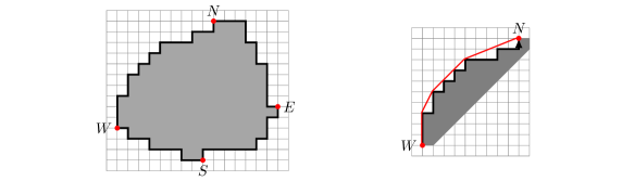
Figure 2: A polyomino composed of $4$ NW-convex. The $W$ to $N$ NW-convex path is coded by $w=1110110101010001001$.

The contour of a DCP is then the union of the four (clockwise) paths $WN$, $NE$, $ES$ and $SW$. Rotating the latter three paths by, respectively, a quarter turn, a half turn, three quarter turn counterclockwise leaves all paths containing only north and east steps; digital convexity is characterized by the fact that each (rotated) side is NW-convex.

Definition 1.3.

A path $p$ is NW-convex if it begins and ends by a north step and if there is no cell between $p$ and its upper convex hull (see Fig. 2).

In the following, we mainly focus on the characterization and random sampling of NW-convex paths.

1.2 Words

The characterization in [9] is based on combinatorics on words. Let us recall some classical notations. We are interested in words on the alphabet $\{0,1\}$. Thus $\{0,1\}^{*}$ is the set of all words, $\{0,1\}^{+}$ is the set of non-empty words.

Each NW-path can be bijectively coded by a word $w\in\{0,1\}^{*}$. From $W$ to $N$, the letter $0$ encodes a horizontal (east) step and $1$ a vertical (north) step (see figure 2).

The idea is to decompose a NW-convex path $w$ by contacts between $w$ and its convex hull.

Definition 1.4.

Let $p$, $q$ be two integers, with $p\geq 0$ and $q>0$. The Christoffel word associated to $p$, $q$ is the word which codes the highest path going from $(0,0)$ to $(p,q)$ while staying under the line going from $(0,0)$ to $(p,q)$. A Christoffel word is primitive if $p$ and $q$ are coprime.

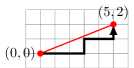
Figure 3: The Christoffel primitive word 0001001, of slope $2/5$.

Note that a Christoffel primitive word always ends with $1$.

1.3 Symbolic characterization of NW-convex paths

Let us recall in this section, two basic notions in analytic combinatorics: the combinatorial classes and the enumerative generating functions.

A combinatorial class is a finite or countable set $\mathcal{C}$, together with a size function $|.|:\mathcal{C}\mapsto\mathbb{N}$ such that, for all $n\in\mathbb{N}$, only a finite number $c_{n}$ of elements of $\mathcal{C}$ have size $n$. The (ordinary) generating function $C(z)$ for the class $\mathcal{C}$ is the formal power series $C(z)=\sum_{n}c_{n}z^{n}=\sum_{\gamma\in\mathcal{C}}z^{|\gamma|}$. If $C(z)$ has a positive (possibly infinite) convergence radius $\rho$ (which is equivalent to the condition that $\overline{\lim}\,c_{n}^{1/n}<\infty$), standard theorems in analysis imply that the power series $C(z)$ converges and defines an analytic function in the complex domain $|z|<\rho$; here we will only use the fact that $C(z)$ is defined for real $0<z<\rho$.

Our sampler is based on the following decomposition theorem.

Theorem 1.5.

[9] A word is NW-convex if and only if it is a sequence of Christoffel primitive words of decreasing slope, beginning with $1$.

The reason of a NW-convex path to begin with a vertical step is to avoid half-turn on the contour of a polyomino. Indeed, since all Christoffel primitive words end with $1$, this ensures compatibility with the standard decomposition (beginning and ending on a corner). Since the Christoffel primitive words appear in decreasing order, NW-convex paths can be identified with multisets of Christoffel primitive words, with the condition that the word $1$ appears at least once in the multiset (this condition can be removed by removing the initial vertical step from NW-convex paths). This is the description we will use in what follows next.

The generating function of Christoffel primitive words, counted by their lengths, is $\sum\limits_{n\geq 1}\varphi(n)z^{n}$, with $\varphi$ the Euler’s totient function. It follows [14, p. 29] that the generating function of the class $\mathcal{S}$ of NW-convex paths, counted by length, is $S(z)=\prod\limits_{n=1}^{\infty}(1-z^{n})^{-\varphi(n)}$. More precisely, we can use the 3-variate generating function $S(z,h,v)=(1-zv)^{-1}\prod\limits_{n=2}^{\infty}\prod\limits_{p+q=n,p\wedge q=1}(1-z^{n}v^{p}h^{q})^{-1}$, to describe by $[z^{n}h^{i}v^{j}]S(z,h,v)$ the number of NW-convex paths beginning in $(0,0)$ and terminating in position $(i,j)$.

2 Asymptotics for NW-convex paths and its limit shape

This section is dedicated to the analysis of some properties of NW-convex paths. The main objective is to describe a limit shape for the normalized random NW-convex paths. This is obtained in three steps. In the first one we extract the asymptotic of NW-convex paths using a Mellin transform approach. In the second one, using the same approach we prove that the asymptotic of the average number of initial vertical steps of a NW-convex path is in $O(\sqrt[3]{n})$. Then, using some technical lemmas, we conclude with the fact that the limit shape is $\sqrt{2z}-z$ with $0\leq z\leq 1/2.$ Let us begin by a brief overview on Mellin transforms. For more details, see [14].

2.1 Brief overview on Mellin transforms

The Mellin transform is an integral transform similar to Laplace transform from which we can derive asymptotic estimates of expressions involving specific infinite products or sums. Given a continuous function $f$ defined on $\mathbb{R}^{+}$, the Mellin transform of $f$ is the function

$$\mathcal{M}[f](s):=\int_{0}^{\infty}f(t)t^{s-1}\mathrm{d}t.$$ (1)

If $f(t)=O(t^{-a})$ as $t\to 0^{+}$ and $f(t)=O(t^{-b})$ as $t\to+\infty$, then $\mathcal{M}[f](s)$ is an analytic function defined on the fundamental strip $a<\mathrm{Re}(s)<b$. In addition, $\mathcal{M}[f](s)$ is in most cases continuable to a meromorphic function in the whole complex plane.

The first fundamental property of the Mellin transform is that it factorizes harmonic sums as follows:

$$G(t)=\sum_{k\geq 1}a_{k}f(\mu_{k}t)\ \Rightarrow\ \mathcal{M}[G](s)=\Big{(}\sum_{k\geq 1}a_{k}\mu_{k}^{-s}\Big{)}\mathcal{M}[f](s).$$ (2)

In a similar way as the Laplace transform, the Mellin transform is almost involutive, the function $f(t)$ being recovered from $\mathcal{M}[f](s)$ using the inversion formula

$$f(t)=\int_{c-i\infty}^{c+i\infty}\mathcal{M}[f](s)t^{-s}\mathrm{d}s\ \ \ \ \mathrm{for\ any\ }c\in(a,b).$$ (3)

From the inversion formula and the residue theorem, the asymptotic expansion of $f(t)$ as $t\to 0^{-}$ can be derived from the poles of $\mathcal{M}[f](s)$ on the left of the fundamental domain, the rightmost such pole giving the dominant term of the asymptotic expansion. If $\mathcal{M}[f](s)$ is decreasing very fast as $\mathrm{Im}(s)\to\infty$ (which occurs in all series to be analyzed next, based on the fact that $\Gamma(s)$ is decaying fast and $\zeta(s)$ is of moderate growth as $\mathrm{Im}(s)\to\infty$), then the following transfer rule holds: a pole of $\mathcal{M}[f](s)$ of order $k\!+\!1$ ($k\geq 0$),

$$\mathcal{M}[f](s)\mathop{\sim}_{s\to\alpha}\lambda_{\alpha}\frac{(-1)^{k}k!}{(s-\alpha)^{k+1}}$$

yields a term

$$\lambda_{\alpha}t^{-\alpha}\ln(t)^{k}$$

in the singular expansion of $f(t)$ around $0$. In particular, a simple pole $\lambda_{\alpha}/(s-\alpha)$ yields a term $\lambda_{\alpha}/t^{\alpha}$.

The first step is to determine the Mellin transform of $\ln(S(e^{-t}))$ which is easier than to obtain that the Mellin transform of $S(z)$. After that it is quite easy to compute the expansion for $S(z)$ when $z$ tends to 1.

Lemma 2.1.

The Mellin transform associated with the series of irreducible discrete segments is

$$\mathcal{M}[\ln(S(e^{-t}))](s)={\frac{\zeta\left(s+1\right)\zeta\left(s-1\right)\Gamma\left(s\right)}{\zeta\left(s\right)}},$$

where $\zeta(z)$ and $\Gamma(z)$ denote the Riemann zeta function and the Gamma function, respectively.

Proof.

The proof relies on an exp-log schema rewriting $\ln(S(e^{-t}))$ as an harmonic sum, and then applying harmonic sum properties. Indeed, by an exp-log schema, we can rewrite $\ln(S(e^{-t}))$ as an harmonic sum. Indeed, we have :

$$\ln(S(e^{-t}))=\sum\limits_{n=1}^{\infty}-\varphi(n)\ln(1-e^{-tn})$$

and by an expansion of $\ln(1-x)$, we get :

$$\ln(S(e^{-t}))=\sum\limits_{n=1}^{\infty}\sum\limits_{k=1}^{\infty}\frac{1}{k}\varphi(n)e^{-tkn}$$

We continue by swapping the sums

$$\ln(S(e^{-t}))=\sum\limits_{k=1}^{\infty}\frac{1}{k}B(kz)$$

with $B(z)=\sum\limits_{n=1}^{\infty}\varphi(n)e^{-nt}.$
With the harmonic property of Mellin transform 2, we see that :

$$\mathcal{M}[\ln(S(e^{-t}))](s)=\zeta(s+1)\mathcal{M}[B](s)$$

But, we can now apply the harmonic property to $B$ and we get

$$\mathcal{M}[B](s)=\dfrac{\zeta(s-1)}{\zeta(s)}\mathcal{M}(e^{-t})(s)$$

And finally, as $\mathcal{M}(e^{-t})(s)=\Gamma(s)$, we obtain :

$$\mathcal{M}[\ln(S(e^{-t}))](s)={\frac{\zeta\left(s+1\right)\zeta\left(s-1\right)\Gamma\left(s\right)}{\zeta\left(s\right)}}$$

∎

Proposition 2.2.

We have the following equivalence for $S(z)$ when $z$ tends to 1:

$$S(z)\sim\dfrac{\exp\left({\frac{6z\zeta\left(3\right)}{{\pi}^{2}\left(1-z\right)^{2}}}\right)}{\left(2\pi(1-z)\right)^{\frac{1}{6}}}\cdot\exp\left({\dfrac{g(1-z)+\zeta\left(3\right)}{2{\pi}^{2}}}-2\,\zeta^{\prime}\left(-1\right)\right),$$

where

$$g(t)=\sum_{r}t^{-r}\Gamma(r)\zeta(r+1)\zeta(r-1)$$

and $r$ runs over the non-trivial zeros of the Riemann zeta function.

$$g(t)=\sum_{r}Res_{s=r}(F(s)),$$ (4)

$$F(s)=\frac{t^{-s}\zeta(s+1)\zeta(s-1)\Gamma(s)}{\zeta(s)},$$ (5)

where the right-hand side of (4) represents the sum of the residuals of $F(s)$ over the non-trivial zeros of the Riemann zeta function.

Proof.

Our argument is similar to that presented by Brigham [8] and Yang [21] in the study of partitions of integers into primes. First, we apply the inversion formula for Mellin transforms to the function from Lemma 1 and obtain

$$\ln{S(e^{-t})}=\frac{1}{2\pi i}\int_{c_{0}-i\infty}^{c_{0}+i\infty}t^{-s}\Gamma(s)\zeta(s+1)\frac{\zeta(s-1)}{\zeta(s)}ds$$

with $c_{0}>2$. As in [8, 21], we now shift the line of integration to the vertical $\Re{(s)}=-c_{1},0<c_{1}<1$, taking into account the residues of the integrand at $s=2,0$ and at the non-trivial zeros of the zeta function. Clearly the residue of the integrand at $s=2$ is $6\zeta(3)/\pi^{2}t^{2}$. The pole at $s=0$ is of second order. To find its residue we use the well-known expansions:

$$\zeta(s+1)=\frac{1}{s}+C+...,$$

$$\Gamma(s)=\frac{1}{s}-C+...$$

$$\zeta(s-1)=\zeta(-1)+\zeta^{\prime}(-1)s+...$$

$$t^{-s}=1-s\ln{t}+...$$

and

$$\frac{1}{\zeta(s)}=-2+2s\ln{(2\pi)}+...,$$

where $C$ denotes the Euler’s constant. Multiplying these series, we obtain that the required residue is $-\frac{1}{6}\ln{t}-2\zeta^{\prime}(-1)-\frac{1}{6}\ln{(2\pi)}$. Finally, the residues at the zeta-zeros are accumulated by the sum

$$\sum_{r}t^{-r}\Gamma(r)\zeta(r+1)\zeta(r-1)=g(t),$$ (6)

where $r$ runs over the non-trivial zeta-zeros . In this way we obtain

$$\ln{S(e^{-t})}=\frac{6\zeta(3)}{\pi^{2}t^{2}}+g(t)-\frac{1}{6}\ln{t}-2\zeta^{\prime}(-1)-\frac{1}{6}\ln{(2\pi)}$$

$$-\frac{1}{2\pi i}\int_{-c_{1}-i\infty}^{-c_{1}+i\infty}t^{-s}\Gamma(s)\zeta(s+1)\frac{\zeta(s-1)}{\zeta(s)}ds.$$

To estimate the last integral we use the following bounds for the zeta and gamma functions: $\zeta(1-c_{1}+iy)\ll\mid y\mid^{c_{1}/2}\ln{\mid y\mid},\zeta(-c_{1}-1+iy)\ll\mid y\mid^{-1/2-c_{1}}\ln{\mid y\mid},\Gamma(-c_{1}+iy)\ll\mid y\mid^{-c_{1}-1/2}e^{-\pi\mid y\mid/2},\mid y\mid\geq y_{0}>0$ (see e.g. [16], p. 25 and p. 492). Finally, we estimate $1/\zeta(s)$ using the well-known representation

$$\zeta(s)=\chi(s)\zeta(1-s),\quad\chi(s)=(2\pi)^{s}/(2\Gamma(s)\cos{(\pi s/2)}).$$ (7)

(see [16, p. 9]). For $s=-c_{1}\pm\mid y\mid$, Stirling’s formula implies that $\mid\chi(-c_{1}\pm\mid y\mid)\mid=(\mid y\mid/(2\pi))^{c_{1}+1/2}(1+O(1/\mid y\mid),\mid y\mid\geq y_{0}>0$. Moreover, $\mid\zeta(1-(-c_{1}+i\mid y\mid)\mid=\mid\zeta(1+c_{1}+i\mid y\mid)\mid\geq(1-\epsilon)\zeta(1+c_{1}),0<\epsilon<1$, by [16, Thm. 9.1, p. 235]. This shows that $1/\zeta(-c_{1}+iy)\ll\mid y\mid^{c_{1}+1/2}$. Hence the integrand is absolutely integrable and the integral tends to $0$ as $t\to 0^{+}$ since

$$\frac{1}{2\pi i}\int_{-c_{1}-i\infty}^{-c_{1}+i\infty}t^{-s}\Gamma(s)\zeta(s+1)\frac{\zeta(s-1)}{\zeta(s)}ds$$

$$\ll t^{c_{1}}\int_{0}^{\infty}e^{-\pi\mid y\mid/2}\mid y\mid^{-(c_{1}+1)/2}\ln^{2}{\mid y\mid}dy\ll t^{c_{1}}.$$

Thus, we finally obtain

$$\ln{S(e^{-t})}=\frac{6\zeta(3)}{\pi^{2}t^{2}}+g(t)-\frac{1}{6}\ln{t}-2\zeta^{\prime}(-1)-\frac{1}{6}\ln{(2\pi)}+o(1),\quad t\to 0^{+}.$$ (8)

The proposition now follows after changing the variable $t$ into $1-z$ and taking exponents from both sides of (8).

We conclude the proof of Proposition 1 with an estimate for the function $g(t)$ as $t\to 0^{+}$. Using (7), one can easily check that

$$\zeta(s-1)=\frac{\zeta(2-s)}{2(2\pi)^{1-s}\sin{(\pi s/2)}\Gamma(s-1)}$$ (9)

We represent $\zeta(s)$ in the denominator of (5) using Hadamard’s factorization theorem [20, p. 30-31] as follows:

$$\zeta(s)=\frac{e^{bs}}{2(s-1)\Gamma(s/2+1)}\prod_{r}\left(1-\frac{s}{r}\right)e^{s/r},$$ (10)

where $b=\frac{1}{6}\ln{(2\pi)}-1-C/2$ and $C$ denotes Euler’s constant. We assume first that the zero $r=\delta+i\gamma$ $(0\leq\delta\leq 1)$ of $\zeta(s)$ is simple (i.e. in (16) $m_{r}=1$). Combining (5), (9) and (10), we obtain

$$(s-r)F(s)=\frac{t^{-s}s^{2}(1-s)\Gamma(s/2)\zeta(s+1)\zeta(2-s)e^{-bs}}{2(2\pi)^{1-s}\sin{(\pi s/2)}\prod_{k\geq 1,r_{k}\neq r}(1-s/r_{k})e^{s/r_{k}}}.$$ (11)

In the last formula we assume that the complex zeros $r_{k}=\delta_{k}+i\gamma_{k}$ of $\zeta(s)$ are arranged in a non-decreasing order of the absolute values of their imaginary parts $\mid\gamma_{k}\mid$; if some absolute values coincide the order between them is taken arbitrarily. Clearly, $0\leq\delta_{k}\leq 1,k=1,2,...$. We shall study the behavior of $(s-r)F(s)$ in a neighborhood of $s=r$, say, $\{s:\mid s-r\mid<\epsilon\}$, where $\epsilon>0$ is small enough. Let us take now a positive number $T$ that satisfies the inequality $T+1/K_{1}\ln{T}<\mid\gamma\mid$, where $K_{1}>0$ will be specified later. Further on, by $K_{1},K_{2},...$ we shall denote some positive constants. We represent the product in the denominator of (11) in the following way:

$$\prod_{k\geq 1,r_{k}\neq r}(1-s/r_{k})e^{s/r_{k}}=\Pi_{1}(s)\Pi_{2}(s),$$

where

$$\Pi_{1}(s)=\prod_{r_{k}\neq r,T\leq\mid\gamma_{k}\mid<T+1}(1-s/r_{k})e^{s/r_{k}},\quad\Pi_{2}(s)=\prod_{r_{k}\neq r,\mid\gamma_{k}\mid\notin[T,T+1)}(1-s/r_{k})e^{s/r_{k}}.$$

It is now clear that (11) can be represented as follows:

$$(s-r)F(s)=\frac{\psi(s)}{\Pi_{1}(s)},$$ (12)

where

$$\psi(s)=\frac{t^{-s}s^{2}(1-s)\Gamma(s/2)\zeta(s+1)\zeta(2-s)e^{-bs}}{2(2\pi)^{1-s}\sin{(\pi s/2)}\Pi_{2}(s)}$$ (13)

is analytic in a neighborhood of $s=r$. Hence $\lim_{s\to r}\psi(s)=\psi(r)$. To estimate $\psi(r)$ we first notice that $\zeta(s)$ has no zeros with real parts equal to $0$ or $1$ (see [20, p. 49]). Hence both $\Re{(r+1)},\Re{(2-r)}\in(1,2)$ and by [16, Thm. 1.9, p. 25],

$$\zeta(r+1)\ll\ln{\mid\gamma\mid},\quad\zeta(2-r)\ll\ln{\mid\gamma\mid}.$$

Furthermore

$$\frac{1}{\mid\sin{(\pi r/2)}\mid}\ll e^{-\pi\mid\gamma\mid/2},\quad\Gamma(r/2)\ll e^{-\pi\mid\gamma\mid/4}$$

and

$$t^{-r}\ll t^{-\theta},$$

where $\theta$ is the least upper bound for the real parts of the zeta-zeros. Finally, $1/\mid\Pi_{2}(r)\mid$ is bounded away from $0$ since the product over those $r_{k}$ satisfying $\mid\gamma_{k}\mid\leq T$ has no zeros in the disc $\{s:\mid s-r\mid<\epsilon\}$ if $\epsilon$ is enough small and the other factors for which $\mid\gamma_{k}\mid>T+1$ are geometric progressions with ratios equal to $\mid r/r_{k}\mid<1$. Combining these estimates with (13), for $\mid s-r\mid<\epsilon$, we obtain

$$\mid\psi(s)\mid\ll t^{-\theta}\mid\gamma\mid^{3}\ln^{2}{\mid\gamma\mid}e^{-3\pi\mid\gamma\mid/4}.$$ (14)

Finally, we have to estimate $\lim_{s\to r}1/\mid\Pi_{1}(s)\mid$. We shall use some basic facts from the theory of the distribution of the zeta-zeros in the critical strip. First, we apply the known fact telling us that, for enough large $T$, the number of the zeta zeros with absolute values of their imaginary parts laying in the interval $[T,T+1)$ is at most $O(\ln{T})$ (see [20, p. 211]). Let $K_{1}$ be the constant in this $O$-estimate. We also use an estimate for the average spacings of two successive zeros of $\zeta(s)$ in a neighborhood of $r=\delta+i\gamma$. It is $\sim 2\pi/\ln{\mid\gamma_{k}\mid}\sim 2\pi\ln{\mid\gamma\mid}$ (see [20, pp. 214, 246]). Finally, it is clear that $\mid r_{k}\mid=\mid\delta_{k}+i\gamma_{k}\mid=O(T)=O(\mid\gamma\mid)$, for $0\leq\delta,\delta_{k}\leq 1$ and $T\leq\gamma,\gamma_{k}<T+1$ whenever $T$ is enough large. Therefore, we have

$$\mid\lim_{s\to r}\Pi_{1}(s)\mid=\prod_{r_{k}\neq r,T\leq\mid\gamma_{k}\mid<T+1}\mid 1-\frac{r}{r_{k}}\mid e^{\Re{(r-r_{k})}}\geq K_{2}\prod_{r_{k}\neq r,T\leq\mid\gamma_{k}\mid<T+1}\frac{\mid r-r_{k}\mid}{\mid r_{k}\mid}$$

$$\geq K_{3}\left(\frac{2\pi}{\ln{\mid\gamma\mid}}\right)^{K_{1}\ln{T}}T^{-K_{1}\ln{T}}\geq K_{4}\left(\frac{\pi}{\mid\gamma\mid\ln{\mid\gamma\mid}}\right)^{K_{1}\ln{\mid\gamma\mid}}\geq K_{5}e^{-K_{6}\ln^{2}{\mid\gamma\mid}}.$$

Combining this estimate with (16) (where $m_{r}=1$) and (12)-(14), we obtain

$$\mid Res_{s=r}(F(s)\mid\ll t^{-\theta}\mid\gamma\mid^{3}\ln^{2}{\mid\gamma\mid}\exp{(\ln^{2}{\mid\gamma\mid}-3\pi\mid\gamma\mid/4)}$$

$$\ll t^{-\theta}e^{-K\mid\gamma\mid},\quad K>0.$$ (15)

Although all known zeros $r$ of $\zeta(s)$ in the critical strip are simple (i.e. $m_{r}=1$), it is not yet known whether this is in fact true. At present, there are only estimates for $m_{r}$ (for recent results in this direction, see [15]). The simplest and oldest estimate seems to be $m_{r}\ll\ln{\mid\gamma\mid}$ (see [20, p. 211]). The proof of the fact that (2.1) is true whenever $m_{r}>1$ is technically more complicated. It should follow the line of reasoning given above. One has to deal with a sum containing $m_{r}=O(\ln{T})$ summands, for $r=\delta+i\gamma,0\leq\delta\leq 1,T\leq\mid\gamma\mid<T+1$. Each of these summands must contain after the differentiation the factor $((s-r)/t)^{m_{r}-j}t^{-s},j=0,1,...,m_{r}-1$. Since both $s-r$ and $t$ tend to $0$, one should to keep a balance in each summand, so that $((s-r)/t)^{m_{r}-j}\ll 1$. For the remaining factors in each summand, estimates similar to those presented above seem to be true. In this way (2.1) can be established.

To obtain the final estimate for $g(t)$, we need to use the bound [20, p. 211]

$$\sum_{r=\delta+i\gamma,T\leq\mid\gamma\mid<T+1}1\ll\ln{T}.$$

Hence, by (4),

$$g(t)\ll\sum_{r=\delta+i\gamma}e^{-K\mid\gamma\mid/2}t^{-\theta}\ll t^{-\theta}.$$

∎

Remark 2.3.

Note that

$$Res_{s=r}(F(s))=\dfrac{1}{(m_{r}-1)!}\lim_{s\to r}\frac{d^{m_{r}-1}}{ds^{m_{r}-1}}((s-r)^{m_{r}}F(s)),$$ (16)

where $m_{r}$ denotes the multiplicity of the zeta zero $r$.

Remark 2.4.

Let $\theta$ denote the least upper bound of the real parts of non-trivial zeros of the Riemann zeta function ($\theta=1/2$ if Riemann hypothesis is true). We also proved that the function $g(t)$ defined above satisfies $g(t)=O(t^{-\theta})$ as $t\to 0$.

As a by-product, the equivalence in Proposition 1 allows us to calculate, using technical approach [13] following saddle point methods, the asymptotic growth of the number of NW-convex paths of size $n$:

Proposition 2.5.

For the number $p_{NW}(n)$ of NW-convex paths of size $n$, we have

$$p_{NW}(n)\sim\alpha n^{-11/18}\exp{\left(\beta n^{2/3}+g\left(\left(\frac{12\zeta(3)}{n\pi^{2}}\right)^{1/3}\right)\right)},$$

with $g(t)=\sum_{r}t^{-r}\Gamma(r)\zeta(r+1)\zeta(r-1)$ where $r$ runs over the non-trivial zeros of the Riemann zeta function and

$$\alpha=\dfrac{1}{6}\,{\frac{{2}^{5/9}{{\rm e}^{{\frac{(5/2)\,\zeta\left(3\right)-2\,\zeta^{\prime}\left(-1\right){\pi}^{2}}{{\pi}^{2}}}}}\sqrt[9]{\zeta\left(3\right)}{3}^{{\frac{11}{18}}}}{{\pi}^{{\frac{8}{9}}}}}\sim 0.3338488807...$$

$$\mbox{and }\beta=\frac{3}{2^{2/3}}\left(\frac{\zeta(3)}{\zeta(2)}\right)^{1/3}=\dfrac{2^{-1/3}3^{4/3}\zeta(3)^{1/3}}{\pi^{2/3}}\sim 1.702263426...$$

Proof.

The function $S(z)$ can be analyze exactly in the same vein that the generating function of integer partitions (see. [14, p574-578]). This explains that we can use saddle point analysis on the approximation of $S(z)$ to obtain the asymptotics of $p_{NW}(n).$ The aim of the proof is to verify the H-admissibility of the function $S(z)$. After that, the calculations are standard and the result ensues.

So, let $x_{n}=1-\left(\frac{12\zeta(3)}{\pi^{2}n}\right)^{1/3}$ be the root of the saddle point equation and let $t_{n}=-\ln{x_{n}}\sim\left(\frac{12\zeta(3)}{\pi^{2}n}\right)^{1/3}$ (i.e., $x_{n}=e^{-t_{n}}$). We shall prove the following decay property:

$$\mid S(x_{n}e^{i\theta})\mid=o(S(x_{n})/\sqrt{b(x_{n})}),\quad n\to\infty,$$ (17)

uniformly for $t_{n}\leq\mid\theta\mid<\pi$.

First we notice that

$$\frac{\mid S(e^{-t_{n}+i\theta})\mid}{S(e^{-t_{n}})}=\exp{(\Re{(\ln{S(e^{-t_{n}+i\theta}}))}-\ln{S(e^{-t_{n}}))}}.$$ (18)

(Here $\ln{(.)}$ denotes the main branch of the logarithmic function, so that $\ln{y}<0$ if $0<y<1$.) Then, setting $\theta=2\pi u$, for $t_{n}/2\pi\leq\mid\theta\mid/2\pi=\mid u\mid<1/2$, we have

$$\Re{(\ln{S(e^{-t_{n}+i\theta}})}-\ln{S(e^{-t_{n}}))}=$$

$$=\Re{\left(-\sum_{k=1}^{\infty}\varphi(k)\ln{\left(\frac{1-e^{-kt_{n}+2\pi iuk}}{1-e^{-kt_{n}}}\right)}\right)}$$

$$=-\frac{1}{2}\sum_{k=1}^{\infty}\varphi(k)\ln{\left(\frac{1-2e^{kt_{n}}\cos{(2\pi uk)}+e^{-kt_{n}}}{(1-e^{kt_{n}})^{2}}\right)}$$

$$=-\frac{1}{2}\sum_{k=1}^{\infty}\varphi(k)\ln{\left(1+\frac{4e^{kt_{n}}\sin^{2}{(\pi uk)}}{(1-e^{kt_{n}})^{2}}\right)}$$

$$\leq-\frac{1}{2}\sum_{k=1}^{\infty}\varphi(k)\ln{(1+4e^{kt_{n}}\sin^{2}{(\pi uk)})}$$

$$\leq-\frac{\ln{5}}{2}\sum_{k=1}^{\infty}\varphi(k)e^{-kt_{n}}\sin^{2}{(\pi uk)}=-\frac{\ln{5}}{2}U_{n},$$ (19)

where the last inequality follows from the fact that $\ln{(1+y)}\geq\frac{\ln{5}}{4}$ for $0\leq y\leq 4$. Further, we shall obtain a bound from below for the sum

$$U_{n}=\sum_{k=1}^{\infty}\varphi(k)e^{-kt_{n}}\sin^{2}{(\pi uk)}.$$ (20)

We also denote by $\{d\}$ the fractional part of the real number $d$, and by $\parallel d\parallel$ the distance from $d$ to the nearest integer, so that

$$\parallel d\parallel=\left\{\begin{array}[]{ll}\{d\}&\qquad\mbox{if}\qquad\{d\}\leq 1/2,\\ 1-\{d\}&\qquad\mbox{if}\qquad\{d\}>1/2.\end{array}\right.$$

It is not difficult to show that

$$\sin^{2}{(\pi d)}\geq 4\parallel d\parallel^{2}$$ (21)

We notice that $\parallel uk\parallel=uk$ if $\mid u\mid k<1/2$, that is, if $k<1/2\mid u\mid\leq\pi/t_{n}$. Hence, applying (21), the inequality $\mid u\mid\geq t_{n}/2\pi$ and the fact that $\varphi(k)\geq c_{0}k/\ln{\ln{k}}$ for $k\geq 3$ (this fact is due to Landau), we obtain

$$U_{n}\geq 4\sum_{k=1}^{\infty}\varphi(k)e^{-kt_{n}}\parallel uk\parallel^{2}$$

$$\geq 4u^{2}\sum_{1\leq k\leq\pi/t_{n}}k^{2}\varphi(k)e^{kt_{n}}\geq\frac{t_{n}^{2}}{\pi^{2}}\sum_{3\leq k\leq\pi/t_{n}}k^{2}\left(c_{0}\frac{k}{\ln{\ln{k}}}\right)e^{kt_{n}}$$

$$\geq\frac{c_{0}t_{n}^{2}}{\ln{\ln{(\pi/t_{n})}}}t_{n}^{-4}\int_{0}^{\pi}y^{3}e^{-y}dy\geq c_{1}\frac{t_{n}^{-2}}{\ln{\mid\ln{t_{n}}\mid}}.$$ (22)

Here $c_{0}$ and $c_{1}$ are positive constants. Replacing (2.1), (20) and (2.1) into (18) and taking into account the asymptotic equivalence for $t_{n}$, we get

$$\mid S(x_{n}e^{i\theta})\mid=O(S(x_{n})\exp{(-c_{3}n^{2/3}/\ln{\ln{n}})}).$$

This implies immediately (17) since $\sqrt{b(x_{n})}$ is of order $const.n^{2/3}$ - much smaller than the exponential one given above.

∎

Remark 2.6.

The contribution of $g\left(\left(\frac{12\zeta(3)}{n\pi^{2}}\right)^{1/3}\right)$ is a fluctuation of very small amplitude as it is classically observe in similar analysis. In particular, this contribution is imperceptible on the first 1000 coefficients.

Now, we focus on the study of the average number of initial vertical steps (which corresponds to the size of the first block of 1 in its associated word) in a NW-convex path.

Lemma 2.7.

The average number of initial steps is equivalent to ${\frac{\sqrt[3]{18{\pi}^{2}n}}{6\sqrt[3]{\zeta\left(3\right)}}}.$

Proof.

A classical way to tackle this type of problem is to mark by a new parameter the contribution of initial steps in the generating function. So, we have the following bivariate generation function $S(z,u)=(1-zu)^{-1}\prod\limits_{n=2}^{\infty}(1-z^{n})^{-\varphi(n)}$ where clearly, the coefficient $[z^{n}u^{k}]S(z,u)$ is the number of NW-convex path of size $n$ having exactly $k$ initial vertical steps. Now, the average number of initial steps for the NW-convex path of size $n$ is just $\dfrac{[z^{n}]\dfrac{\partial S(z,u)}{\partial u}|_{u=1}}{[z^{n}]S(z,1)}$. So, we need to extract the asymptotic of $G(z):=\dfrac{\partial S(z,u)}{\partial u}|_{u=1}=\dfrac{z}{(1-z)^{2}}\prod\limits_{n=2}^{\infty}(1-z^{n})^{-\varphi(n)}$. Again, we proceed by a Mellin transform approach and we get that:

$$\mathcal{M}[\ln(G(e^{-t}))](s)={\frac{\zeta\left(s+1\right)(\zeta\left(s-1\right)+\zeta\left(s\right))\Gamma\left(s\right)}{\zeta\left(s\right)}}$$

So, $G(z)\sim\dfrac{\exp\left({\frac{6z\zeta\left(3\right)}{{\pi}^{2}\left(1-z\right)^{2}}}\right)}{\left(2\pi(1-z)^{7}\right)^{\frac{1}{6}}}\cdot\exp\left({\dfrac{g(1-z)+\zeta\left(3\right)}{2{\pi}^{2}}}-2\,\zeta^{\prime}\left(-1\right)\right).$ Finally, using saddle point analysis and dividing by the asymptotic of $p_{NW}(n)$, we obtain lemma 2.7.

∎

In particular, if we renormalize the NW-convex path by $1/n$, the contribution of the initial steps for the limit shape is null.

Now, we are interested in the average position of the terminating point of a random NW-convex path. If we consider NW-convex path without their initial vertical steps, then by symmetry, we can conclude that the average ending position is $(x_{n}\sim\frac{n}{2},y_{n}\sim\frac{n}{2})$. But by lemma 2.7 and the fact that the length of the renormalized initial vertical steps is $o(1)$, it follows that:

Lemma 2.8.

The average position of the ending point of a random NW-convex path of size $n$ is $(x_{n}\sim\frac{n}{2},y_{n}\sim\frac{n}{2}).$

Following the same approach, with a little more work, we can prove that:

Proposition 2.9.

The average abscissa of the point of slope $x$ in a renormalized by $1/n$ NW-convex path of size $n$ is $\dfrac{1}{2}\left(1-\left(\dfrac{x}{1+x}\right)^{2}\right).$

Proof.

From lemma 2.8 we deduce:

$$\dfrac{\partial(1-zv)S(z,h,v)}{\partial h}|_{h=1,v=1}=\dfrac{z}{2}\dfrac{\partial(1-zv)S(z,h,v)}{\partial z}|_{h=1,v=1},$$

Additionally, expanding of the derivative, we have

$$\dfrac{\partial(1-zv)S(z,h,v)}{\partial h}|_{h=1,v=1}=(1-zv)S(z,h,v)|_{h=1,v=1}\sum\limits_{n=2}^{\infty}\sum\limits_{p+q=n,p\wedge q=1}\dfrac{pz^{n}}{1-z^{n}}.$$

So, we deduce from this the following technical lemma which will be useful in the sequel:

Lemma 2.10.

The following identity holds:

$$\sum\limits_{n=2}^{\infty}\dfrac{z^{n}}{1-z^{n}}\sum\limits_{p+q=n,p\wedge q=1}p=\sum\limits_{n=2}^{\infty}\dfrac{n\varphi(n)z^{n}}{2(1-z^{n})}=\dfrac{z}{2}\dfrac{\dfrac{\partial(1-zv)S(z,h,v)}{\partial h}|_{h=1,v=1}}{(1-zv)S(z,h,v)|_{h=1,v=1}}.$$

Let us continue with the average position of the point of slope $x$ for $0\leq x<\infty$. The position of the ending point, previously done, is a special case of this question (where $x=0$). For that purpose, let us consider the generating function

$$F_{x}(z,u)=(1-z)^{-1}\prod\limits_{n=2}^{\infty}\prod\limits_{p+q=n,p\wedge q=1,\frac{q}{p}>x}(1-z^{n}u^{p})^{-1}\prod\limits_{p+q=n,p\wedge q=1,\frac{q}{p}\leq x}(1-z^{n})^{-1}.$$

The average abscissa of the point of slope $x$ in a NW-convex path of size $n$ is nothing but the expectation $\dfrac{[z^{n}]\dfrac{\partial F_{x}(z,u)}{\partial u}|_{u=1}}{[z^{n}]F_{x}(z,1)}.$ Expanding the derivative, we get:

$$\dfrac{\partial F_{x}(z,u)}{\partial u}|_{u=1}=F_{x}(z,u)|_{u=1}\sum\limits_{n=2}^{\infty}\dfrac{z^{n}}{1-z^{n}}\sum\limits_{p+q=n,p\wedge q=1,\frac{q}{p}>x}p.$$

Now, we need the following short number theory lemma:

Lemma 2.11.

The following equivalence holds for every fixed $x\in[0,\infty[$:
$\sum\limits_{p+q=n,p\wedge q=1,\frac{q}{p}>x}p=\dfrac{1}{2}\left(1-\left(\dfrac{x}{1+x}\right)^{2}\right)n\varphi(n)(1+\varepsilon(n))$ with $\varepsilon(n)\rightarrow 0$ as $n$ tends to $\infty$.

The proof is quite immediate.

Finally, using the lemma 2.10, we get proposition 2.9. ∎

At this stage, to prove that the limit shape is deterministic, we need to show that the standard deviation of the abscissa is in $o(n)$. This proof is long and technical, but follows the same way that we do for the expectation. We conclude by solving the differential equation: $\left\{f\left(0\right)=0,2f\left(z\right)=1-{\frac{\left({\frac{d}{dz}}f\left(z\right)\right)^{2}}{\left(1+{\frac{d}{dz}}f\left(z\right)\right)^{2}}}\right\}$ which explains the fact that the slope of $f(z)$ is $x$ at the abscissa $\dfrac{1}{2}\left(1-\left(\dfrac{x}{1+x}\right)^{2}\right).$ Consequently, we have:

Theorem 2.12.

The limit shape for the renormalized by $1/n$ NW-convex path of size $n$ as $n$ tends to the infinity is the curve of equation $f(z)=\sqrt{2z}-z$.

3 Boltzmann samplers for NW-convex paths

Boltzmann samplers have been introduced in 2004 by Duchon et al. [11] as a general framework to generate uniformly at random specifiable combinatorial structures. These samplers are very efficient, their expected complexity is typically linear. In comparison with the recursive method of sampling, the principle of Boltzmann samplers essentially deals with evaluations of the generating function of the structures, and avoids counting coefficient (which need to be pre-computed in the recursive method). Quite a few papers have been written to extend and optimize Boltzmann samplers [19, 3, 6, 5, 7, 2, 4].

Consequently, we choose Boltzmann sampling for the class of digitally convex polyominoes. After a short introduction to the method, we analyze the complexity of the sampler. This part is based on an analysis by Mellin transform techniques.

3.1 A short introduction to Boltzmann samplers

Let us recall the definitions and the main ideas of Boltzmann sampling.

Definition 3.1.

Let $\mathcal{A}$ be a combinatorial class and $A(x)$ its ordinary generating function. A (free) Boltzmann sampler with parameter $x$ for the class $\mathcal{A}$ is a random algorithm $\Gamma_{x}\mathcal{A}$ that draws each object $\gamma\in\mathcal{A}$ with probability:

$$\mathbb{P}_{x}(\gamma)=\frac{x^{|\gamma|}}{A(x)}.$$

Notice that this definition is consistent only if $x$ is a positive real number taken within the disk of convergence of the series $A(x)$.

The great advantage of choosing the Boltzmann distribution for the output size is to allow simple and automatic rules to design Boltzmann samplers from a specification of the class.

Note that from free Boltzmann samplers, we easily define two variants: the exact-size Boltzmann sampler and the approximate-size one, just by rejecting the inappropriate outputs until we obtain respectively a targeted size or a targeted interval of type $[(1-\varepsilon)n,(1+\varepsilon)n]$. In order to optimize this rejection phase, it is crucial to tune efficiently the parameter $x$. A good choice is generally to take the unique positive real solution $x_{n}$ (or an approximation of it when $n$ tends to infinity) of the equation $\dfrac{xA^{\prime}(x)}{A(x)}=n$ which means that the expected size of the output tuned by $x_{n}$ equals $n$.

To conclude, let us recall that authors of the seminal paper [11] distinguished a special case where Boltzmann samplers are particularly efficient (and we prove in the sequel, that we are in this situation). This case arises when the Boltzmann distribution of the output is bumpy, that is to say, when the following conditions are satisfied:

• $\mu_{1}(x)\rightarrow\infty$ when $x\rightarrow\rho^{-}$

• $\sigma(x)/\mu_{1}(x)\rightarrow 0$ when $x\rightarrow\rho^{-},$

where $\mu_{1}(x)$ (resp. $\sigma^{2}(x)$) is the expected size (resp. the variance) of the output, and $\rho$ is the dominant singularity of $A(x)$.

3.2 The class of the digitally convex polyominoes

Let us recall that the digitally convex polyominoes can be decomposed into four NW-convex paths, each of them being a multiset of discrete irreducible segments. Moreover, according to the previous section, we have a specification for the discrete irreducible segments in terms of word theory. This brings us the generating function associated to a NW-convex path:

$$S(z)=\prod\limits_{n=1}^{\infty}(1-z^{n})^{-\varphi(n)},$$

where $\varphi(n)$ designs the Euler’s totient function.

The first question that occurs concerns the determination of the parameter $x_{n}$ which is a central point for the tuning of the sampler. In order to approximate $x_{n}$ as $n$ tends to infinity, we need to apply the asymptotic of $S(z)$ as $z\rightarrow 1$, we already calculate for the asymptotic of the NW-convex paths.

3.3 The Boltzmann distribution of the NW-convex paths

The first step to analyze the complexity of exact- and approximate-size Boltzmann sampler is to characterize the type of the Boltzmann distribution. In this subsection we prove that the Boltzmann distribution is bumpy. This ensures that we only need on average a constant number of trials to draw an object of approximate-size. Moreover, a precise analysis allows us to give the complexity of the exact-size sampling.

Firstly, we derive from the equivalence of $S(z)$ close to its dominant singularity $\rho=1$, an expression for the tuning of the Boltzmann parameter:

Corollary 3.2.

A good choice for the Boltzmann parameter $x_{n}$ in order to draw a large NW-convex paths of size $n$ is $x_{n}=1-\sqrt[3]{{\dfrac{12\zeta\left(3\right)}{n{\pi}^{2}}}}.$

Proof.

The expected size of the output is $\dfrac{xS^{\prime}(x)}{S(x)}$ which is an increasing function in $x$. Using the equivalent of $S(x)$ when $x$ tends to 1, we can approximate the first member of the equation $\dfrac{xS^{\prime}(x)}{S(x)}=n$ to obtain $\dfrac{12\zeta\left(3\right)}{\left(1-x\right)^{3}{\pi}^{2}}=n.$ The result ensues immediately. ∎

So, the first condition for the bumpy distribution is clearly verified. We now focus our attention on the fraction $\sigma(x)/\mu_{1}(x)$.

Lemma 3.3.

The expected size of the Boltzmann output satisfies:

$$\mu_{1}(x)\sim\dfrac{12\zeta\left(3\right)}{\left(1-x\right)^{3}{\pi}^{2}}\mbox{ as }x\mbox{ tends to 1.}$$

The variance of the size of the Boltzmann output satisfies:

$$\sigma(x)\sim\frac{6\,\sqrt{\zeta\left(3\right){{x}}}}{\pi{\left(1-x\right)^{2}}}\mbox{ as }x\mbox{ tends to 1.}$$

So, the Boltzmann distribution of the NW-convex paths is bumpy.

Finally, we describe the sampler for digitally convex polyominoes. This needs some care during the stage when we glue the NW-convex paths together.

3.4 Random sampler to draw Christoffel primitive words

We now look more precisely how to implement the samplers. Firstly, we address the question of drawing two coprime integers which is non-classical in Boltzmann sampling, from which we derive a Boltzmann sampler for NW-convex paths. The first step to generate NW-convex paths is to draw Christoffel primitive words with Boltzmann probability. We recall that this is equivalent to draw two coprime integers $p,q$ with probability $\frac{x^{p+q}}{\sum_{n\geq 1}\varphi(n)x^{n}}$.

Let $b(x,n):=\dfrac{\varphi(n)x^{n}}{\sum\limits_{n=1}^{\infty}{\varphi(n)x^{n}}}$. The following algorithm is an elementary way to answer the question posed above:

Input: a parameter $x$

Output: Two coprime integers

Draw $n$ with Boltzmann probability $b(x,n)$

Do Draw $p$ uniformly in $\{1,...,n\}$

While $p,n$ not coprime

return $(p,n-p)$

Algorithm 1 $\Gamma_{CP}$

The average complexity of the algorithm is in $O(n\ln\ln(n))$.

6

6

6

6

6

6

3.4.1 Correctness

$p\wedge n=1\Leftrightarrow p\wedge n-p=1$, so drawing $p$ coprime with $n$ uniformly in $\{1,..,n\}$ is equivalent to draw uniformly $p,q$ coprime with $p+q=n$. With the choice of $n$ with the probability $\frac{\varphi(n)x^{n}}{\sum\limits_{n=1}^{\infty}{\varphi(n)x^{n}}}$, we obtain a Boltzmann sampler for Christoffel primitive words.

3.4.2 Complexity

To evaluate the complexity of this sampler there are two steps of the algorithm that should be analyzed: the drawing of $n$ with probability $b(x,n)$ and the drawing of two coprime numbers. The drawing of $n$ is essentially related to the generating function evaluation and to $\varphi(k)$ for all $k\leq n$. In the following, we consider that both the generating function and a table for large enough $\varphi(n)$ are to be precomputed. So, the complexity of the drawing of $n$ is in $O(n)$. Experimentally, the precomputation takes a couple of minutes on a standard personal computer. Now let us evaluate the complexity of drawing the coprime numbers. The probability for $p$ to be taken uniformly from $\{1,..,n\}$ being also coprime with $n$ is $\varphi(n)/n$ and the following classical inequality [1, Thm 8.8.7] on totient’s function:
$\dfrac{\varphi(n)}{n}>\dfrac{1}{e^{\gamma}\log\log(n)+\dfrac{3}{\ln\ln(n)}}$ (valid for all positive integers $n$) proves that on average the number of trials in the loop is $O(\log\log(n))$.

Remark 3.4.

In fact, we can expect a better complexity. Indeed, with Boltzmann probability, we have better chance to draw an integer $n$ such that $\varphi(n)$ is close to $n$ and in this case the probability to draw a coprime $p$ is positive.

3.5 Random sampler drawing a NW-convex path

To draw a NW-convex path, we use the isomorphism between NW-convex paths and multisets of Christoffel primitive words. The multiset is a classical constructor, for which its Boltzmann sampler in the unlabelled case had been given in [12]. The idea is to draw with an appropriate distribution (called IndexMax distribution) an integer $M$, and then draw a random number of Christoffel primitive words with a Boltzmann sampler of parameter $x^{i}$ and to replicate each drawn object $i$ times, for all $1\leq i\leq M$. Well chosen probabilities ensures the Boltzmann distribution.

Once we get a multiset of pairs of coprime integers, we can transform it into a NW-convex path coded on $\{0,1\}$ as follows:

• Draw a multiset $m$ in $\operatorname{\textsc{MSet}}(PC)$,

• Sort the elements $(p,q)$ of $m$ in decreasing order according to $q/p$,

• Transform each element into the discrete line of slope $q/p$ coded on $\{0,1\}$,

• add a $1$ at the beginning.

Clearly, this transformation has a complexity in $O(n\ln(n))$, due to the sorting.

3.6 Complexity of sampling a NW-convex path in approximate and exact size

The previous sections bring all needed elements to determine the complexity of the Boltzmann sampler for a NW-convex path. The two following theorems respectively tackle the complexity of the sampling in the case of approximate-size output or exact size output.

Theorem 3.5.

An approximate-size Boltzmann sampler for NW-convex paths succeeds in one trial with probability tending to 1 as $n$ tends to infinity. The overall cost of approximate-size sampling is $O(n\ln(n))$ on average.

Theorem 3.6.

An exact-size Boltzmann sampler for NW-convex paths succeeds in mean number of trials tending to $\kappa\cdot n^{2/3}$ with $\kappa={\dfrac{\sqrt[6]{2}\sqrt[3]{3}{\pi}^{5/6}}{\sqrt[6]{\zeta\left(3\right)}}}\approx 4.075517917...$ as $n$ tends to infinity. The overall cost of exact-size sampling is $O(n^{5/3}\ln(\ln(n)))$ on average.

Remark 3.7.

Since $\varphi(n)$ grows slowly, the parameter $x_{n}$ tuned to draw large objects will be close to $1$, which gives big replication orders. A consequence is that we do not need to calculate the generating function of primitive Christoffel words to a huge order to have a good approximation of our probabilities.

3.7 Random sampler drawing digitally convex polyominoes

We can now sample independent NW-convex paths with Boltzmann probability. We want to obtain an entire polyomino by gluing four (rotated) NW-convex path.
However, gluing a 4-tuple of NW-convex paths, we do not necessarily obtain the contour of a polyomino. Indeed, we need the following extra conditions: the four NW-convex paths should be non-crossing, and they need to form a closed walk with no half-turn.

Input: a parameter $x$

Output: a quadruple of compatible NW-convex paths.

Repeat:

      Draw WN, NE, ES, SW using independent calls to a Boltzmann sampler of

      NW-convex path of parameter $x$.

      If $|WN|_{0}+|NE|_{1}=|ES|_{0}+|SW|_{1}$ and $|NE|_{0}+|ES|_{1}=|SW|_{0}+|WN|_{1}$

      then return $(WN,NE,ES,SW)$

Algorithm 2 $\Gamma_{P}$

5

5

5

5

5

The non-crossing and no half-turn conditions are trivially satisfied when the four paths are NW-convex. Then the closing problem stays and we need to add a rejection phase at this step. More precisely, to be closed, we need to have as much horizontal steps in the upper part from W to E as in the lower part from E to W, and as much vertical steps in the left part from S to N as in the right part from N to S. A naive way to sample DCP according to a Boltzmann distribution is presented in Algorithm 2. A more efficient uniform sampler can probably be adapted from [2] and is currently under development.

Figure 4: To the left, a random polyomino of perimeter 81109 drawn with parameter $x=0.98$. To the right perimeter distribution of a NW-convex path drawn with $x=0.8908086616$.

Conclusion

We proposed in this paper an effective way to draw uniformly at random digitally convex polyominoes. Our approach is based on Boltzmann generators which allows us to build large digitally convex polyomioes. These samples point out the fact that random digitally convex polyominoes admit a limit shape as their size tends to infinity. The limit shape of the NW-convex paths we proved in this paper seems to be also the limit shape for NW part of the digitally convex polyominoes. The tools to tackle it are for the moment beyond our reach. Even, the simpler question of a precise asymptotic enumeration of the digitally convex polyominoes (the order of magnitude is proven [17]) is currently a challenge. We conclude by noting that our work could certainly be extended to higher dimensions. But, this is a work ahead…

Acknowledgement

The fourth author established the collaboration on this work during his visit at LIPN, University of Paris 13. He wishes to thank for the fruitful discussions, hospitality and support. We thank Axel Bacher for its English corrections. Olivier Bodini is supported by ANR project MAGNUM, ANR 2010 BLAN 0204.

References

- [1] E. Bach and J. Shallit. Algorithmic number theory. Vol. 1. Foundations of Computing Series. MIT Press, Cambridge, MA, 1996. Efficient algorithms.
- [2] O. Bodini, D. Gardy, and O. Roussel. Boys-and-girls birthdays and hadamard products. Fundam. Inform., 117(1-4):85–101, 2012.
- [3] O. Bodini and A. Jacquot. Boltzmann Samplers For Colored Combinatorial Objects. In Proceedings of Gascom’08, 2008.
- [4] O. Bodini and J. Lumbroso. Dirichlet random samplers for multiplicative combinatorial structures. In 2012 Proceedings of the Eigth Workshop on Analytic Algorithmics and Combinatorics (ANALCO), pages 92–106, Kyoto, Japan, 2012.
- [5] O. Bodini and Y. Ponty. Multi-dimensional boltzmann sampling of languages. DMTCS Proceedings, 0(01):49–64, 2010.
- [6] Olivier Bodini, Olivier Roussel, and Michèle Soria. Boltzmann samplers for first-order differential specifications. Discrete Applied Mathematics, 160(18):2563–2572, 2012.
- [7] M. Bodirsky, E. Fusy, M. Kang, and S. Vigerske. An unbiased pointing operator for unlabeled structures, with applications to counting and sampling. In Proceedings of the eighteenth annual ACM-SIAM symposium on Discrete algorithms, SODA ’07, pages 356–365, Philadelphia, PA, USA, 2007. Society for Industrial and Applied Mathematics.
- [8] N.A. Brigham. On a certain weighted partition function. Proc. Amer. Math. Soc., 1:192–204, 1950.
- [9] S. Brlek, J.-O. Lachaud, X. Provencal, and C. Reutenauer. Lyndon christoffel digitally convex. Pattern Recognition, 42(10):2239 – 2246, 2009.
- [10] David Coeurjolly, Serge Miguet, and Laure Tougne. Discrete curvature based on osculating circle estimation. In Proceedings of the 4th International Workshop on Visual Form, IWVF-4, pages 303–312, London, UK, UK, 2001. Springer-Verlag.
- [11] P. Duchon, P. Flajolet, G. Louchard, and G. Schaeffer. Boltzmann samplers for the random generation of combinatorial structures. Combinatorics, Probablity, and Computing, 13(4–5):577–625, 2004. Special issue on Analysis of Algorithms.
- [12] P. Flajolet, E. Fusy, and C. Pivoteau. Boltzmann sampling of unlabelled structures. In SIAM Press, editor, Proceedings of ANALCO’07 (Analytic Combinatorics and Algorithms) Conference, volume 126, pages 201–211, 2007.
- [13] P. Flajolet, B. Salvy, and P. Zimmermann. Automatic average-case analysis of algorithm. Theoretical Computer Science, 79(1):37–109, 1991.
- [14] P. Flajolet and R. Sedgewick. Analytic Combinatorics. Cambridge University Press, 2009.
- [15] A. Ivić. On the multiplicity of zeros of the zeta-function. Acad. Serbe des Sciences et Arts, Bull. CXVIII Class. des Sci. Math. et naturelles, Sci. Math., No. 24, Belgrade, pages 119–132, 1999. available at arXiv:math/0501434vl [math.NT], January, 2005.
- [16] A. Ivić. The Riemann zeta-function: theory and applications. Dover Books on Mathematics. Dover, 2003.
- [17] A. Ivic, Jack Koplowitz, and Jovisa D. Zunic. On the number of digital convex polygons inscribed into an (m, m)-grid. IEEE Transactions on Information Theory, 40(5):1681–1686, 1994.
- [18] B. Kerautret, J. O. Lachaud, and B. Naegel. Comparison of discrete curvature estimators and application to corner detection. In Proceedings of the 4th International Symposium on Advances in Visual Computing, ISVC ’08, pages 710–719, Berlin, Heidelberg, 2008. Springer-Verlag.
- [19] C. Pivoteau, B. Salvy, and M. Soria. Boltzmann oracle for combinatorial systems. In Algorithms, Trees, Combinatorics and Probabilities, pages 475–488. Discrete Mathematics and Theoretical Computer Science, 2008. Proceedings of the Fifth Colloquium on Mathematics and Computer Science. Blaubeuren, Germany. September 22-26, 2008.
- [20] E.C. Titchmarsh. The Theory of the Riemann Zeta-Function. The Clarendon Press, Oxford University Press, 1986. New York.
- [21] Y. Yang. Partitions into primes. Trans. Amer. Math. Soc., 352:2581–2600, 2000.