Weak decay constant of neutral pions in a hot and magnetized quark matter

Abstract

The directional weak decay constants of neutral pions are determined at finite temperature $T$, chemical potential $\mu$ and in the presence of a constant magnetic field $B$. To do this, we first derive the energy dispersion relation of neutral pions from the corresponding effective action of a two-flavor, hot and magnetized Nambu–Jona-Lasinio model. Using this dispersion relation, including nontrivial directional refraction indices, we then generalize the PCAC relation of neutral pions and derive the Goldberger-Treiman (GT) as well as the Gell–Mann-Oakes-Renner (GOR) relations consisting of directional quark-pion coupling constant $g_{qq\pi^{0}}^{(\mu)}$ and the weak decay constant $f_{\pi^{0}}^{(\mu)}$ of neutral pions. The temperature dependence of $g_{qq\pi^{0}}^{(\mu)}$ and $f_{\pi^{0}}^{(\mu)}$ are then determined for fixed chemical potential and various constant background magnetic fields. The GT and GOR relations are also verified at finite $T,\mu$ and $eB$. It is shown that, because of the explicit breaking of the Lorentz invariance by the magnetic field, the directional quark-pion coupling and decay constants of neutral pions in the longitudinal and transverse directions with respect to the direction of the external magnetic field are different, i.e., $g_{qq\pi^{0}}^{\|}\neq g_{qq\pi^{0}}^{\perp}$ and $f_{\pi^{0}}^{\|}\neq f_{\pi^{0}}^{\perp}$. As it turns out, for fixed $T,\mu$ and $B$, $g_{qq\pi^{0}}^{\|}>g_{qq\pi^{0}}^{\perp}$ and $f_{\pi^{0}}^{\|}<f_{\pi^{0}}^{\perp}$.

I Introduction

Today’s theory of strong interactions is quantum chromodynamics (QCD). At momentum scales of several GeV, QCD is a theory of weakly interacting quarks and gluons. At low momentum scales, however, QCD is governed by color confinement, which is accompanied by spontaneous breaking of chiral symmetry. According to the Goldstone theorem, spontaneous chiral symmetry breaking (S$\chi$SB) implies the existence of Nambu-Goldstone (NG) bosons. For two quark flavors, up and down, the isospin triplet of neutral and charged pions is identified as the NG bosons of S$\chi$SB. Thus, at low momentum scales, the weakly interacting pions build up the main degrees of freedom of QCD. There is strong theoretical and experimental evidence that chiral symmetry is restored at temperatures higher than $200$ MeV. Crucial information on the restoration of chiral symmetry is provided by the change in the pion properties in the vicinity of the chiral transition point. Among these properties, the pions’ mass, $m_{\pi}$, and weak decay constant, $f_{\pi}$, are the most important quantities, since they are deeply related to S$\chi$SB: $m_{\pi}$ and $f_{\pi}$ are related to the quark bare mass and the chiral condensate via the Gell–Mann-Oakes-Renner (GOR) relation weise2012 ; nam2008 . To study the properties of pions, models of Nambu–Jona-Lasinio (NJL) type have been quite useful buballa2004 . One of the basic properties of these models is that they include a gap equation that connects the chiral condensate and the dynamical quark mass. This provides a mechanism for dynamical chiral symmetry breaking and the generation of quark quasiparticle masses weise2009 . It is known that strong magnetic fields enhance this dynamical mass generation via the phenomenon of magnetic catalysis klimenko1992 ; miransky1995 . Different aspects of the effect of strong magnetic fields on the properties of quark matter were recently summarized in kharzeev2012 (see, in particular, catalysis ).

In our previous paper fayazbakhsh2012 , we have investigated the effect of external magnetic fields on the properties of neutral pions in a hot quark matter. In particular, the neutral pion mass and its directional refraction indices have been computed by making use of the effective action of a bosonized two-flavor NJL model in the presence of a constant magnetic field. We have shown that, since the presence of constant background magnetic fields breaks the Lorentz invariance, a certain anisotropy emerges in the refraction indices of neutral pions in the transverse and longitudinal directions with respect to the direction of the external magnetic field. In the present paper, we will mainly focus on the effect of external magnetic fields on the weak decay constant of neutral pions at finite temperature. We will show that this quantity exhibits the same anisotropy in the presence of constant background magnetic fields. Modifying the PCAC relation, we will also prove the Goldberger-Treiman (GT) and GOR relations in the presence of external magnetic fields. The effect of a constant background magnetic field on the low energy relations of neutral pions was previously studied in agasian2001 . Using a first order chiral perturbation theory, it was shown that $f_{\pi^{0}}$ and $m_{\pi^{0}}$ are shifted in such a way that the GOR relation remains valid at finite $T$ and $eB$ agasian2001 .

Very strong magnetic fields are supposed to be created in the early stages of noncentral heavy-ion collisions at the RHIC and LHC rhicmagnetic . Depending on the collision energies and impact parameters, these magnetic fields are estimated to be of the order $eB\sim 1.5m_{\pi}^{2}$, with $m_{\pi}=138$ MeV, corresponding to $0.03$ GeV², and $eB\sim 15m_{\pi}^{2}$, corresponding to $0.3$ GeV², respectively skokov2010 . Although extremely short lived, the strong magnetic fields created in the heavy-ion collisions affect the properties of charged quarks in the early stage of the collision. Consequently, the properties of pions, even neutral pions, which are made of these magnetized quarks are affected by background magnetic fields. Let us emphasize that neutral pions cannot interact directly with the external magnetic fields, because of the lack of electric charge. Our method provides a possibility to study the effect of strong magnetic fields on neutral pions, at least at a theoretical level. Studying the properties of neutral pions in the final freeze-out region may provide some hints on the prehistory of their constituent quarks in the early stages of heavy-ion collisions.

The organization of this paper is as follows: In Sec. II, we will introduce the two-flavor magnetized NJL model, and, reviewing our analytical results from fayazbakhsh2012 , we will derive the effective action of neutral scalar and pseudoscalar mesons, $\sigma\sim\bar{\psi}\psi$ and $\pi^{a}\sim\bar{\psi}i\gamma_{5}\tau^{a}\psi$, in a derivative expansion up to the second derivative. We will show that it includes nontrivial form factors. To study the dynamics of pions, we will mainly focus on the kinetic part of the effective action that implies a nontrivial “anisotropic” energy dispersion relation for neutral pions,

$$E_{\pi^{0}}^{2}=u_{\pi^{0}}^{(i)2}q_{i}^{2}+m_{\pi^{0}}^{2}.$$ (I.1)

Here, $u_{\pi^{0}}^{(i)},i=1,2,3$ are the directional refraction indices and $m_{\pi^{0}}$ is the mass of neutral pions. We then present our numerical results for the $T$ dependence of $u_{\pi^{0}}^{(i)},i=1,2,3$ and $m_{\pi^{0}}$ for fixed magnetic fields $eB=0.03,0.2,0.3$ GeV² and zero chemical potential.

Comparing this case with the case of zero temperature and/or magnetic field, we arrive at following conclusions: Starting with an isospin symmetric theory at zero temperature and in a magnetic-field-free vacuum, the refraction indices for all pions are given by

$$u_{\pi_{a}}^{(i)}=1,\qquad\forall i,a=1,2,3.$$ (I.2)

Thus, according to (I.1), the energy dispersion relation of neutral pions in field-free vacuum turns out to be the well-known “isotropic” energy-dispersion relation

$$E_{\pi^{a}}^{2}={\mathbf{q}}^{2}+m_{\pi^{a}}^{2},\qquad\forall a=1,2,3.$$ (I.3)

Hence, in the chiral limit, and in field-free vacuum, massless pions propagate at the speed of light.

At finite temperature, and $eB=0$, however, the relativistic invariance of the theory is broken by the medium, but the isospin symmetry is still preserved. In this case a single refraction index is defined for all pions by

$$u_{\pi_{a}}^{(1)}=u_{\pi_{a}}^{(2)}=u_{\pi_{a}}^{(3)}=u,\qquad\forall a=1,2,3.$$ (I.4)

The energy dispersion relation (I.1) is therefore given by $E_{\pi_{a}}^{2}=u^{2}{\mathbf{q}}^{2}+m_{\pi_{a}}^{2}$, for all $a=1,2,3$. This relation appears e.g. in shuryak1990 ; son2000 ; ayala2002 . According to the results in son2000 ; ayala2002 , the refraction index $u$, being a $T$-dependent quantity, is always smaller than unity (i.e. $u<1$). Thus, as it turns out, in the chiral limit, massless pions move at a speed slower than the speed of light pisarski1996 ; chiral-perturbation .

In fayazbakhsh2012 , we have studied the case $T\neq 0$ and $eB\neq 0$, and shown that the effect of the magnetic field is twofold: First, the isospin symmetry of the theory breaks down. Consequently, neutral and charged pions exhibit different properties in the presence of background magnetic fields. Second, for a magnetic field aligned in a fixed direction, a certain anisotropy appears in the transverse and longitudinal directions with respect to this fixed direction. In fayazbakhsh2012 , we have only considered the case of neutral pions, and we assumed that the magnetic field is directed in the third direction. Here, the above-mentioned anisotropy is reflected in the directional refraction indices as fayazbakhsh2012

$$u_{\pi^{0}}^{(1)}=u_{\pi^{0}}^{(2)}\neq u_{\pi^{0}}^{(3)}.$$ (I.5)

Thus, the magnetized neutral pions satisfy the anisotropic energy dispersion relation (I.1). Within our truncation up to second order derivative expansion, the transverse refraction indices $u_{\pi^{0}}^{(1)}=u_{\pi^{0}}^{(2)}>1$, and the longitudinal one $u_{\pi^{0}}^{(3)}=1$, and they do not depend on temperature and/or magnetic fields [see Fig. 4(b) in Sec. II]. As concerns the chiral limit, it turns out that whereas the massless pions propagate in the direction parallel to the magnetic field with the speed of light, their velocity in the plane perpendicular to the direction of the $B$ field is larger than $1$. The natural question arising at this stage is how these results are reflected in the other properties of neutral and massive pions, in particular, in their low energy relations. In Secs. III-IV of the present paper, we have tried to answer this question by computing the “directional” weak decay constant of neutral pions using a modified PCAC relation, that leads naturally to modified GT and GOR relations.

In Sec. III, we prove the GT and GOR relations in two different cases: In Sec. III.1, using the main arguments presented in buballa2004 , we will first assume that the pions satisfy the ordinary isotropic energy dispersion relation (I.3). We will then combine the ordinary PCAC relation

$$\langle 0|J_{\mu,5}^{a}(0)|\pi^{b}(q)\rangle=f_{\pi}q_{\mu}\delta^{ab},$$ (I.6)

and the Feynman integral corresponding to the one-pion-to-vacuum matrix element, and then derive the ordinary GT as well as GOR relations

$$g_{qq\pi}f_{\pi}=m+{\cal{O}}(m_{0}^{2}),$$ (I.7)

as well as

$$m_{\pi}^{2}f_{\pi}^{2}=\frac{m_{0}\sigma_{0}}{2G}+{\cal{O}}(m_{0}^{2}).$$ (I.8)

Here, $J_{\mu,5}^{a}\equiv\bar{\psi}\gamma_{\mu}\gamma_{5}\lambda^{a}\psi$, with $\lambda^{a}=\tau^{a}/2$, is the axial vector current, $g_{qq\pi}$ is the quark-pion coupling constant, $m=m_{0}+\sigma_{0}$ is the constituent quark mass, including the bare quark mass $m_{0}$, and the chiral condensate $\sigma_{0}=-2G\langle\bar{\psi}\psi\rangle$, with $G$ being the NJL coupling constant. In Sec. III.2, we will then generalize the method presented in Sec. III.1 to the case of pions satisfying anisotropic energy dispersion relation (I.1). To derive the modified GT and GOR relations in this case, we will appropriately modify the PCAC relation as

$$\langle 0|J_{\mu,5}^{a}(0)|\pi^{b}(q)\rangle=f_{b}q_{\mu}u_{\pi_{b}}^{(\mu)2}\delta^{ab},$$ (I.9)

for all $\mu=0,\cdots,3$ and $a,b=1,2,3$. Here, the four-vector $u_{\pi_{b}}^{(\mu)}\equiv(1,u_{\pi_{b}}^{(i)})$, with $u_{\pi_{b}}^{(i)},i=1,2,3$ the directional refraction indices appearing in (I.1). In (I.9), $f_{b}$ is first an unknown dimensionful proportionality factor, which will then be shown to be equal to the constituent quark mass $m$. Following the same method as in Sec. III.1, we will derive the modified GT and GOR relations for all $\mu=0,\cdots,3$ and $a=1,2,3$ as

$$g_{qq\pi_{a}}^{(\mu)}f_{\pi_{a}}^{(\mu)}=m+{\cal{O}}(m_{0}^{2}),$$ (I.10)

and

$$m_{\pi_{a}}^{2}f_{\pi_{a}}^{(\mu)2}=u_{\pi_{a}}^{(\mu)2}\frac{m_{0}\sigma_{0}}{2G}+{\cal{O}}(m_{0}^{2}),$$ (I.11)

which, in contrast to (I.7) and (I.8), include the “directional” quark-pion coupling $g_{qq\pi^{0}}^{(\mu)}$ and weak decay constants of neutral pions $f_{\pi_{a}}^{(\mu)}$, as well as the directional refraction indices $u_{\pi_{a}}^{(\mu)}$. Note that for $\mu=0$ (temporal direction), the GOR relation (I.11) leads to the well-known GOR relation

$$m_{\pi_{a}}^{2}f_{\pi_{a}}^{(0)2}=\frac{m_{0}\sigma_{0}}{2G}+{\cal{O}}(m_{0}^{2}),$$ (I.12)

arising at finite temperature and zero magnetic field pisarski1996 ; chiral-perturbation . As aforementioned, the case of a nonvanishing magnetic field can be viewed as a special case, where neutral pions satisfy the anisotropic energy dispersion relation (I.1) with directional refraction indices given in (I.5). In Sec. IV, we will explicitly determine $g_{qq\pi^{0}}^{(\mu)}$ and $f_{\pi_{a}}^{(\mu)}$, first analytically (see Sec. IV.1) and then numerically (see Sec. IV.2). As it turns out, $g_{qq\pi^{0}}^{(0)}=g_{qq\pi^{0}}^{(3)}\neq g_{qq\pi^{0}}^{(1)}=g_{qq\pi^{0}}^{(2)}$, as well as $f_{\pi^{0}}^{(0)}=f_{\pi^{0}}^{(3)}\neq f_{\pi^{0}}^{(1)}=f_{\pi^{0}}^{(2)}$. In studying the $T$ dependence of these quantities, we arrive at $g_{qq\pi^{0}}^{(0)}>g_{qq\pi^{0}}^{(1)}\qquad\mbox{and}\qquad f_{\pi^{0}}^{(0)}<f_{\pi^{0}}^{(1)}$. Setting $a=3$ in the GT and GOR relations (I.10) and (I.11), we will use these relations for neutral pions to prove numerically that $f_{3}$, appearing in (I.9), is given by the constituent quark mass $m$. Using the numerical data for $m_{\pi^{0}}^{2}$, $f_{\pi^{0}}^{(\mu)}$, $u_{\pi^{0}}^{(\mu)}$ and $m$, we will compare numerically the left- and right hand side (r.h.s.) of the relation

$$m_{\pi_{a}}^{2}f_{\pi_{a}}^{(\mu)2}=u_{\pi_{a}}^{(\mu)2}\frac{m_{0}m}{2G},$$ (I.13)

which, comparing to the original GOR relation (I.11), includes the contributions of ${\cal{O}}(m_{0}^{2})$. As it turns out, this relation seems to be exact for small $T$ and $eB$. A slight deviation from this relation occurs at temperature above the chiral transition temperature. In Sec. V, we will summarize our results. A number of useful relations, which are used to derive the analytical results in Sec. IV, are presented in the Appendix.

II The Model

II.1 Effective action of a two-flavor magnetized NJL model in a derivative expansion

Let us start with the Lagrangian density of a two-flavor gauged NJL model

$${\cal{L}} = \bar{\psi}(x)\left(i\gamma^{\mu}D_{\mu}-m_{0}\right)\psi(x)+G~{}\{[\bar{\psi}(x)\psi(x)]^{2}$$ (II.1)

$$+[\bar{\psi}(x)i\gamma_{5}\vec{\tau}\psi(x)]^{2}\}-\frac{1}{4}F^{\mu\nu}F_{\mu\nu}.$$

Here, $\psi_{\alpha,f}^{c},\bar{\psi}_{\alpha,f}^{c}$ are the fermionic fields, carrying Dirac $\alpha\in(1,\cdots,4)$, flavor $f\in(1,2)=(u,d)$ and color $c\in(1,2,3)=(r,g,b)$ indices. Choosing the bare quark mass $m_{0}\equiv m_{u}=m_{d}$, the above Lagrangian density is invariant under $SU(2)$ isospin symmetry. The global $SU_{L}(2_{f})\times SU_{R}(2_{f})$ chiral and $SU(3_{c})$ color symmetries are guaranteed in the chiral limit $m_{0}\to 0$. Fixing the external $U(1)$ gauge field, $A_{\mu}^{\mbox{\tiny{ext.}}}$, appearing in the covariant derivative $D_{\mu}\equiv\partial_{\mu}+ieQA_{\mu}^{\mbox{\tiny{ext.}}}$, as $A_{\mu}^{\mbox{\tiny{ext.}}}=\left(0,0,Bx_{1},0\right)$, a constant magnetic field is produced, which is directed in the third direction, $\mathbf{B}=B\mathbf{e}_{3}$. Here, $Q=\mbox{diag}\left(2/3,-1/3\right)$ is the charge matrix of the up and down quarks. Using $A_{\mu}^{\mbox{\tiny{ext.}}}$, the electromagnetic field strength tensor$F_{\mu\nu}\equiv\partial_{[\mu}A_{\nu]}^{\mbox{\tiny{ext.}}}$ is a constant tensor, with the only nonvanishing component $F_{12}=-F_{21}=B$. Defining the auxiliary meson fields $\sigma$ and $\vec{\pi}$ as

$$\sigma(x) = -2G\bar{\psi}(x)\psi(x),$$

$$\vec{\pi}(x) = -2G\bar{\psi}(x)i\gamma_{5}\vec{\tau}\psi(x),$$ (II.2)

where $\vec{\tau}=(\tau_{1},\tau_{2}.\tau_{3})$ are the Pauli matrices, the Lagrangian density (II.1) is equivalently given by the semibosonized Lagrangian as

$${\cal{L}}_{sb} = \bar{\psi}(x)\left(i\gamma^{\mu}D_{\mu}-m_{0}\right)\psi(x)-\bar{\psi}\left(\sigma+i\gamma_{5}\vec{\tau}\cdot\vec{\pi}\right)\psi$$ (II.3)

$$-\frac{(\sigma^{2}+\vec{\pi}^{2})}{4G}-\frac{B^{2}}{2}.$$

The effective action corresponding to (II.3), $\Gamma_{\mbox{\tiny{eff}}}$, is then determined by integrating out the fermionic fields $\psi$ and $\bar{\psi}$,

$$e^{i\Gamma_{\mbox{\tiny{eff}}}[\Phi(x)]}=\int{\cal{D}}\psi{\cal{D}}\bar{\psi}\exp\left(i\int d^{4}x~{}{\cal{L}}_{sb}\right).$$ (II.4)

As a functional of $x$-dependent meson fields

$$\Phi(x)=\left(\varphi_{0},\varphi_{1},\varphi_{2},\varphi_{3}\right)\equiv\left(\sigma,\pi_{1},\pi_{2},\pi_{3}\right),$$ (II.5)

the effective action $\Gamma_{\mbox{\tiny{eff}}}$ consists of two parts, $\Gamma_{\mbox{\tiny{eff}}}=\Gamma_{\mbox{\tiny{eff}}}^{(0)}+\Gamma_{\mbox{\tiny{eff}}}^{(1)}$. The tree-level part is given by

$$\Gamma_{\mbox{\tiny{eff}}}^{(0)}[\Phi(x)]=-\int d^{4}x\left(\frac{\sigma^{2}+\vec{\pi}^{2}}{4G}+\frac{B^{2}}{2}\right),$$ (II.6)

and the one-loop part reads

$$\Gamma_{\mbox{\tiny{eff}}}^{(1)}[\Phi(x)]=-i{\mbox{tr}}_{\{sfcx\}}\ln(i{S_{Q}^{-1}[\Phi(x)]}).$$ (II.7)

Here, the trace operation includes a trace over discrete degrees of freedom, spinor $s$, flavor $f$ and color $c$, as well as an integration over the continuous coordinate $x$. The inverse fermion propagator appearing in (II.7) is given by

$$iS^{-1}_{Q}[\Phi(x)]\equiv i\gamma^{\mu}D_{\mu}-\big{[}m(x)+i\gamma^{5}\vec{\tau}\cdot\vec{\pi}(x)\big{]},$$ (II.8)

with $m(x)\equiv m_{0}+\sigma(x)$. In what follows, we use the method used in fayazbakhsh2012 to evaluate the effective action $\Gamma_{\mbox{\tiny{eff}}}[\Phi(x)]$ in a derivative expansion up to second order. To do this, let us assume a constant field configuration $\Phi_{0}\equiv\left(\sigma_{0},\mathbf{0}\right)$ that breaks the $SU_{L}(2_{f})\times SU_{R}(2_{f})$ chiral symmetry of the original action in the chiral limit. We then expand $\Phi(x)$ around this constant configuration,

$$\Phi(x)=\Phi_{0}+\bar{\Phi}(x).$$ (II.9)

Plugging (II.9) into the effective action $\Gamma_{\mbox{\tiny{eff}}}[\Phi(x)]$, we arrive first at

$$\Gamma_{\mbox{\tiny{eff}}}[\Phi]=\Gamma_{\mbox{\tiny{eff}}}[\Phi_{0}]-\frac{1}{2}\int d^{d}x\ {\cal{M}}^{2}_{ij}[\Phi_{0}]\bar{\varphi}_{i}(x)\bar{\varphi}_{j}(x)$$ (II.10)

$$+\frac{1}{2}\int d^{d}x\ \chi_{ij}^{\mu\nu}[\Phi_{0}]\partial_{\mu}\bar{\varphi}_{i}(x)\partial_{\nu}\bar{\varphi}_{j}(x)+\cdots,$$

where the summation over $i,j=0,\cdots,3$ is skipped. Here, the squared mass matrix ${\cal{M}}_{ij}^{2}$ and the kinetic matrix $\chi_{ij}^{\mu\nu}$ are given by

$${\cal{M}}_{ij}^{2}[\Phi_{0}] \equiv -\int d^{d}z\frac{\delta^{2}\Gamma_{\mbox{\tiny{eff}}}}{\delta\varphi_{i}(0)\delta\varphi_{j}(z)}\bigg{|}_{\Phi_{0}},$$ (II.11)

$$\chi_{ij}^{\mu\nu}[\Phi_{0}] \equiv -\frac{1}{2}\int d^{d}zz^{\mu}z^{\nu}\frac{\delta^{2}\Gamma_{\mbox{\tiny{eff}}}}{\delta\varphi_{i}(0)\delta\varphi_{j}(z)}\bigg{|}_{\Phi_{0}}.$$ (II.12)

Choosing, at this stage, the kinetic matrix $\chi_{ij}^{\mu\nu}$, as in miransky1995 ; fayazbakhsh2012 , in the form

$$\chi_{ij}^{\mu\nu}[\Phi]=(F_{1}^{\mu\nu})_{ij}+2F_{2}^{\mu\nu}\frac{\varphi_{i}\varphi_{j}}{\Phi^{2}},\hskip 14.22636pt\forall i,j=0,\cdots,3,$$

with $\Phi^{2}=\sigma^{2}+\vec{\pi}^{2}$, and plugging (II.1) into (II.10), the kinetic part of the effective action, $\Gamma_{\mbox{\tiny{eff}}}^{k}[\Phi]$, will then be given by $\Gamma_{\mbox{\tiny{eff}}}^{k}[\Phi]=\int d^{d}x~{}{\cal{L}}_{k}[\Phi]$, where ${\cal{L}}_{k}[\Phi]$ is the part of the effective Lagrangian including only two derivatives,

$${\cal{L}}_{k}=\frac{1}{2}(F_{1}^{\mu\nu})_{ij}\partial_{\mu}\varphi_{i}\partial_{\nu}\varphi_{j}+\frac{F_{2}^{\mu\nu}}{\Phi^{2}}\left(\varphi_{i}\partial_{\mu}\varphi_{i}\right)\left(\varphi_{j}\partial_{\nu}\varphi_{j}\right).$$

Here, according to (II.5), the fields $\varphi_{i},i=1,\cdots,3$ are identified by the meson fields $\sigma$ and $\vec{\pi}$. Following the standard algebraic manipulations presented in fayazbakhsh2012 , the effective action of the two-flavor NJL model including $\sigma,\vec{\pi}$ mesons, which is valid in a truncation of the effective action up to two derivatives, reads

$$\Gamma_{\mbox{\tiny{eff}}}[\sigma,\vec{\pi}]=\Gamma_{\mbox{\tiny{eff}}}[\sigma_{0}]$$ (II.15)

$$-\frac{1}{2}\int d^{d}x~{}\bar{\sigma}(x)\left(M_{\sigma}^{2}+{\cal{G}}^{\mu\mu}\partial_{\mu}^{2}\right)\bar{\sigma}(x)$$

$$-\frac{1}{2}\sum\limits_{\ell=1}^{3}\int d^{d}x~{}\bar{\pi}_{\ell}(x)\left(M_{\vec{\pi}}^{2}+{\cal{F}}^{\mu\mu}\partial_{\mu}^{2}\right)_{\ell\ell}\bar{\pi}_{\ell}(x).$$

For a constant field configuration $\sigma_{0}$, $\Gamma_{\mbox{\tiny{eff}}}[\sigma_{0}]$ is given by $\Gamma_{\mbox{\tiny{eff}}}[\sigma_{0}]=-{\cal{V}}\Omega_{\mbox{\tiny{eff}}}$, where ${\cal{V}}$ denotes the four-dimensional space-time volume and $\Omega_{\mbox{\tiny{eff}}}$ is the effective (thermodynamic) potential. In fayazbakhsh2012 , the thermodynamic potential of this model is derived at finite temperature $T$, finite chemical potential $\mu$, and in the presence of constant magnetic field $B$. It reads

$$\Omega_{\mbox{\tiny{eff}}}(m;T,\mu,eB)=\frac{\sigma_{0}^{2}}{4G}+\frac{B^{2}}{2}-\frac{3}{2\pi^{2}}\sum\limits_{q\in\{\frac{2}{3},-\frac{1}{3}\}}|q_{f}eB|^{2}\left\{\zeta^{\prime}\left(-1,x_{q_{f}}\right)+\frac{x_{q_{f}}^{2}}{4}+\frac{x_{q_{f}}}{2}(1-x_{q_{f}})\ln x_{q_{f}}\right\}$$ (II.16)

$$+\frac{3}{4\pi^{2}}\left\{m^{4}\ln\left(\frac{\Lambda+\sqrt{\Lambda^{2}+m^{2}}}{m}\right)-\Lambda(2\Lambda^{2}+m^{2})\sqrt{\Lambda^{2}+m^{2}}\right\}$$

$$-3T\sum\limits_{q_{f}\in\{\frac{2}{3},-\frac{1}{3}\}}|q_{f}eB|\sum^{+\infty}_{p=0}\alpha_{p}\int_{-\infty}^{+\infty}\frac{dp_{3}}{4\pi^{2}}\left\{\ln\left(1+e^{-\beta(E_{q}+\mu)}\right)+\ln\left(1+e^{-\beta(E_{q}-\mu)}\right)\right\}.$$

In a mean field approximation, the constant field configuration $\Phi_{0}=(\sigma_{0},\mathbf{0})$ is supposed to minimize the above thermodynamic potential $\Omega_{\mbox{\tiny{eff}}}$. In (II.16), $m=m_{0}+\sigma_{0}$, $x_{q_{f}}\equiv\frac{m^{2}}{2|q_{f}eB|}$, $\Lambda$ is an appropriate ultraviolet (UV) momentum cutoff and $\beta\equiv T^{-1}$. Moreover, $\zeta^{\prime}(-1,x_{q})\equiv\frac{d\zeta(s,x_{q})}{ds}\big{|}_{s=1}$, where $\zeta(s,a)\equiv\sum_{p=0}^{\infty}(a+p)^{-s}$ is the Riemann-Hurwitz $\zeta$-function, and $\alpha_{p}\equiv 2-\delta_{p,0}$ is the spin degeneracy factor. In (II.16), $E_{q}$ is the energy of charged fermions in a constant magnetic field, which is given by

$$E_{q}\equiv\sqrt{\bar{\mathbf{p}}_{q}^{2}+m^{2}}=\sqrt{2|q_{f}eB|p+p_{3}^{2}+m^{2}}.$$ (II.17)

It arises from the solution of the Dirac equation in the presence of a constant magnetic field using the Ritus eigenfunction method ritus . Here, $\bar{p}_{q}$ is the Ritus four-momentum defined by

$$\bar{p}_{q}=(p_{0},0,-\mbox{sgn}(q_{f}eB)\sqrt{2|q_{f}eB|p},p_{3}),$$ (II.18)

where $p=0,1,2,\cdots$ labels the Landau levels. Using the standard definition (II.11), the squared mass matrices of $\sigma$ and $\vec{\pi}$ mesons, $M_{\sigma}^{2}$ and $(M_{\vec{\pi}}^{2})_{\ell m}$, appearing in (II.15), are defined by

$$M_{\sigma}^{2} \equiv -\int d^{4}z\frac{\delta^{2}\Gamma_{\mbox{\tiny{eff}}}}{\delta\sigma(0)\delta\sigma(z)}\bigg{|}_{(\sigma_{0},{\mathbf{0}})},$$

$$(M_{\vec{\pi}}^{2})_{\ell m} \equiv -\int d^{4}z\frac{\delta^{2}\Gamma_{\mbox{\tiny{eff}}}}{\delta\pi_{\ell}(0)\delta\pi_{m}(z)}\bigg{|}_{(\sigma_{0},{\mathbf{0}})},$$ (II.19)

$\forall\ell,m=1,2,3$. The nontrivial form factors ${\cal{G}}^{\mu\nu}$ and ${\cal{F}}^{\mu\nu}_{\ell m}$, appearing in (II.15), are combinations of the form factors $(F_{\alpha}^{\mu\nu})_{ij},\alpha=1,2,$ and $i,j=0,\cdots,3$, appearing in (II.1). They are defined by ${\cal{G}}^{\mu\nu}\equiv\big{[}(F_{1}^{\mu\nu})_{00}+2F_{2}^{\mu\nu}\big{]}$ and ${\cal{F}}^{\mu\nu}_{\ell m}\equiv\frac{1}{2}\big{[}(F_{1}^{\mu\nu})_{\ell m}+(F_{1}^{\mu\nu})_{m\ell}\big{]}$. They can be determined from the kinetic part of the effective action $\Gamma_{\mbox{\tiny{eff}}}^{k}$ using

$${\cal{G}}^{\mu\nu} \equiv -\frac{1}{2}\int d^{4}zz^{\mu}z^{\nu}\frac{\delta^{2}\Gamma_{\mbox{\tiny{eff}}}^{k}}{\delta\sigma(0)\delta\sigma(z)}\bigg{|}_{(\sigma_{0},{\mathbf{0}})},$$

$${\cal{F}}^{\mu\nu}_{\ell m} \equiv -\frac{1}{2}\int d^{4}zz^{\mu}z^{\nu}\frac{\delta^{2}\Gamma_{\mbox{\tiny{eff}}}^{k}}{\delta\pi_{\ell}(0)\delta\pi_{m}(z)}\bigg{|}_{(\sigma_{0},{\mathbf{0}})},$$ (II.20)

$\forall\ell,m=1,2,3$. Note that, according to our results in fayazbakhsh2012 , the pion mass squared matrix $(M^{2}_{\vec{\pi}})_{\ell m}$ and the form factors ${\cal{G}}^{\mu\nu}$ and ${\cal{F}}^{\mu\nu}_{\ell m}$ have the following properties:

$$(M^{2}_{\vec{\pi}})_{\ell m}=-(M^{2}_{\vec{\pi}})_{m\ell},~{}~{}~{}\mbox{and}~{}~{}~{}{\cal{F}}^{\mu\nu}_{\ell m}=-{\cal{F}}^{\mu\nu}_{m\ell},$$ (II.21)

$\forall\ell\neq m$. Moreover, $\forall\ell,m=1,2,3$, ${\cal{F}}^{\mu\nu}_{\ell m}={\cal{F}}^{\mu\mu}_{\ell m}g^{\mu\nu}$. The latter property is also shared by ${\cal{G}}^{\mu\nu}$.

In the present paper, as in fayazbakhsh2012 , we are mainly interested in the properties of neutral $\sigma$ and $\pi^{0}$ mesons in hot and magnetized quark matter. We therefore identify the $\pi_{3}$ meson with the neutral meson $\pi^{0}$. To simplify the notations in the rest of this paper, we will denote $(M_{\vec{\pi}}^{2})_{33}$ from (II.1) by $M_{\pi^{0}}^{2}$ and ${\cal{F}}^{\mu\nu}_{33}$ from (II.1) by ${\cal{F}}^{\mu\nu}$. Plugging the effective action $\Gamma_{\mbox{\tiny{eff}}}$ from (II.6) and (II.7) in (II.1) and (II.1), the squared mass matrices of neutral mesons, $M_{\sigma}^{2}$ and $M_{\pi^{0}}^{2}$, as well as the form factors ${\cal{G}}^{\mu\nu}$ and ${\cal{F}}^{\mu\nu}$ at zero $(T,\mu)$ and in the presence of a background $B$ field, are given by

$$M_{\sigma}^{2} = \frac{1}{2G}-i\int d^{4}z\mbox{tr}_{sfc}\big{[}S_{Q}(z,0)S_{Q}(0,z)\big{]},$$

$$M_{\pi^{0}}^{2} = \frac{1}{2G}+i\int d^{4}z\mbox{tr}_{sfc}\big{[}S_{Q}(z,0)\tau_{3}\gamma^{5}S_{Q}(0,z)\gamma^{5}\tau_{3}\big{]},$$

and

$${\cal{G}}^{\mu\nu} = -\frac{i}{2}\int d^{4}zz^{\mu}z^{\nu}\mbox{tr}_{sfc}\big{[}S_{Q}(z,0)S_{Q}(0,z)\big{]},$$

$${\cal{F}}^{\mu\nu} = \frac{i}{2}\int d^{4}zz^{\mu}z^{\nu}\mbox{tr}_{sfc}\big{[}S_{Q}(z,0)\tau_{3}\gamma^{5}S_{Q}(0,z)\gamma^{5}\tau_{3}\big{]}.$$

Here, $S_{Q}(x,y)$ is the Ritus fermion propagator fayazbakhsh2012 ; fukushima2009 ,

$$S_{Q}(x,y)=i\sum_{p=0}^{\infty}\int{\cal{D}}\tilde{p}~{}e^{-i\tilde{p}\cdot(x-y)}P_{p}(x_{1})D_{Q}^{-1}(\bar{p})~{}P_{p}(y_{1}),$$

with ${\cal{D}}\tilde{p}\equiv\frac{dp_{0}dp_{2}dp_{3}}{(2\pi)^{3}}$, $\tilde{p}=(p_{0},0,p_{2},p_{3})$, and $\bar{p}$ is the Ritus momentum,

$$\bar{p}=(p_{0},0,-s_{Q}\sqrt{2|QeB|p},p_{3}),$$

with $s_{Q}\equiv\mbox{sgn}(QeB)$. Having in mind that $Q$ is a diagonal matrix with the entries $q_{f}=\{2/3,-1/3\}$, we will use $s\equiv\mbox{sgn}(q_{f}eB)$ for the elements of this $2\times 2$ matrix $s_{Q}$. In (II.1),

$$P_{p}(x_{1}) \equiv \frac{1}{2}[f_{p}^{+s}(x_{1})+\Pi_{p}f_{p}^{-s}(x_{1})]$$ (II.25)

$$+\frac{is_{Q}}{2}[f_{p}^{+s}(x_{1})-\Pi_{p}f_{p}^{-s}(x_{1})]\gamma^{1}\gamma^{2}.$$

Here, $\Pi_{p}\equiv 1-\delta_{p,0}$ considers the spin degeneracy in the lowest Landau level with $p=0$. Moreover, $f_{p}^{\pm s}(x_{1})$ are defined by

$$\begin{array}[]{rclcrcl}f_{p}^{+s}(x_{1})&\equiv&\phi_{p}\left(x_{1}-s_{Q}p_{2}\ell_{B}^{2}\right),&&p&=&0,1,2,\cdots,\\ f_{p}^{-s}(x_{1})&\equiv&\phi_{p-1}\left(x_{1}-s_{Q}p_{2}\ell_{B}^{2}\right),&&p&=&1,2,3,\cdots,\end{array}$$ (II.27)

where $\phi_{p}(x)$ is a function of Hermite polynomials $H_{p}(x)$ in the form

$$\phi_{p}(x)\equiv a_{p}\exp\left(-\frac{x^{2}}{2\ell_{B}^{2}}\right)H_{p}\left(\frac{x}{\ell_{B}}\right).$$ (II.29)

Here, $a_{p}\equiv(2^{p}p!\sqrt{\pi}\ell_{B})^{-1/2}$ is the normalization factor and $\ell_{B}\equiv|QeB|^{-1/2}$ is the magnetic length. In (II.1), $D_{Q}(\bar{p})\equiv\gamma\cdot\bar{p}_{Q}-m$, with $\bar{p}_{Q}$ the Ritus four-momentum from (II.18). Note that since $Q=\mbox{diag}\left(2/3,-1/3\right)$ is a $2\times 2$ matrix in the flavor space, building the trace in the flavor space is equivalent to evaluating the sum over $q_{f}\in\{2/3,-1/3\}$.

In fayazbakhsh2012 , the squared mass matrices of neutral bosons $(M_{\sigma}^{2},M_{\pi^{0}}^{2})$ as well as the nontrivial form factors $({\cal{G}}^{\mu\nu},{\cal{F}}^{\mu\nu})$, appearing in (II.15), are determined numerically at finite $(T,\mu)$ and $eB$. To introduce $T$ and $\mu$, we used the standard replacements

$$p_{0}=i\omega_{n}-\mu,~{}~{}\mbox{and}~{}~{}\int\frac{dp_{0}}{2\pi}\to iT\sum_{n},$$ (II.30)

where $\omega_{n}\equiv(2n+1)\pi T$ are the fermionic Matsubara frequencies. As it turns out, at finite temperature and zero magnetic field, the meson form factors satisfy

$${\cal{G}}^{00} = -{\cal{G}}^{11}=-{\cal{G}}^{22}=-{\cal{G}}^{33},$$

$${\cal{F}}^{00} = -{\cal{F}}^{11}=-{\cal{F}}^{22}=-{\cal{F}}^{33}.$$ (II.31)

For nonvanishing magnetic fields, however, they exhibit a certain anisotropy arising from the explicit breaking of Lorentz invariance by the background magnetic field directed in the third direction,

$${\cal{G}}^{00}=-{\cal{G}}^{33}\neq{\cal{G}}^{11}={\cal{G}}^{22},$$

$${\cal{F}}^{00}=-{\cal{F}}^{33}\neq{\cal{F}}^{11}={\cal{F}}^{22}.$$ (II.32)

II.2 Pole and screening masses of neutral mesons and their directional refraction indices:
A review of our previous numerical results

The effective action $\Gamma_{\mbox{\tiny{eff}}}[\sigma,\vec{\pi}]$ from (II.15) can be used to determine the energy dispersion relations of neutral $\sigma$ and $\pi^{0}$ mesons, which are generically denoted by $M$,

$$E_{M}^{2}=u_{M}^{(i)2}q_{i}^{2}+m_{M}^{2},~{}~{}~{}M\in\{\sigma,\pi^{0}\}.$$ (II.33)

Here, $u_{M}^{(i)},i=1,2,3$ are the directional refraction indices in the spatial $i=1,2,3$ directions. They are defined by

$$u_{\sigma}^{(i)}\equiv\bigg{|}\frac{\mbox{Re}{\cal{G}}^{ii}}{\mbox{Re}{\cal{G}}^{00}}\bigg{|}^{1/2},\qquad u_{\pi^{0}}^{(i)}\equiv\bigg{|}\frac{\mbox{Re}{\cal{F}}^{ii}}{\mbox{Re}{\cal{F}}^{00}}\bigg{|}^{1/2}.$$ (II.34)

Moreover, $m_{M}$ is the neutral mesons’ pole mass given by

$$m_{\sigma}\equiv\bigg{|}\frac{\mbox{Re}M_{\sigma}^{2}}{\mbox{Re}{\cal{G}}^{00}}\bigg{|}^{1/2},\qquad m_{\pi^{0}}\equiv\bigg{|}\frac{\mbox{Re}M_{\pi^{0}}^{2}}{\mbox{Re}{\cal{F}}^{00}}\bigg{|}^{1/2}.$$ (II.35)

In the above relations, the squared mass matrices of neutral mesons $(M_{\sigma}^{2},M_{\pi^{0}}^{2})$, as well as form factors ${\cal{G}}^{\mu\nu}$ and ${\cal{F}}^{\mu\nu}$, are defined in (II.1) as well as (II.1). Combining the refraction indices (II.34) and the pole masses (II.35), the screening masses of neutral mesons are defined by

$$m_{M}^{(i)}=\frac{m_{M}}{u_{M}^{(i)}},~{}\mbox{for}~{}M\in\{\sigma,\pi^{0}\},~{}\mbox{and}~{}i=1,2,3.$$ (II.36)

In fayazbakhsh2012 , we used (II.34)-(II.36) and determined the $T$ dependence of the neutral mesons’ pole and screening masses as well as their refraction indices for vanishing and nonvanishing $\mu$ and $eB$. To do this, we first determined the $T$ dependence of $\sigma_{0}$, the minima of the thermodynamic potential $\Omega_{\mbox{\tiny{eff}}}$ from (II.16). In Fig. 1, the $T$ dependence of the constituent quark mass $m=m_{0}+\sigma_{0}$ is plotted for fixed $\mu=0$ MeV and $eB=0,0.2,0.5$ GeV². We observe that, for a fixed temperature, the constituent quark mass increases with increasing $eB$. Moreover, it turns out that the transition from the broken chiral symmetry phase, with $m\neq 0$, to the normal phase, with $m\simeq m_{0}\approx 0$, is a smooth crossover, and for stronger magnetic fields the transition to the normal phase occurs at higher temperatures. All these effects are related to the phenomenon of magnetic catalysis klimenko1992 ; miransky1995 , according to which the constant magnetic field enhances the production of the chiral condensate $\sigma_{0}\sim\langle\bar{\psi}\psi\rangle$, and therefore catalyzes the dynamical chiral symmetry breaking.

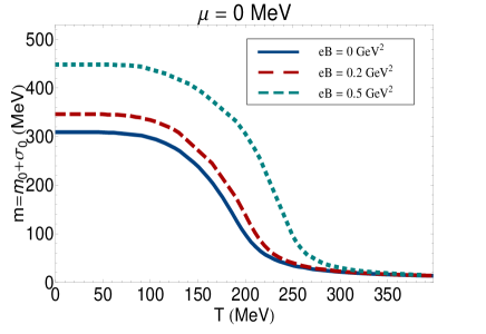
Figure 1: The $T$ dependence of constituent quark mass $m=m_{0}+\sigma_{0}$ for fixed $eB=0,0.2,0.5$ GeV² and fixed $\mu=0$. Here, $m_{0}\simeq 5$ MeV is the bare quark mass and $\sigma_{0}$ is the chiral condensate.

To determine $m_{\sigma}$ and $m_{\pi^{0}}$, we further developed in fayazbakhsh2012 the necessary technique to analytically evaluate the integrals (II.1) and (II.1) up to an integration over the $p_{3}$ momentum and a summation over Landau levels and eventually performed them numerically. In Fig. 2, the $T$ dependence of $m_{\sigma}$ and $m_{\pi_{\ell}},\ell=1,2,3$ is plotted for vanishing $\mu$ and $eB$. The free parameters of the theory, $m_{0},\Lambda$ and $G$, are chosen so that they reproduce the pion mass $m_{\pi}=137.7$ MeV and $m_{\sigma}\simeq 824.3$ MeV, for vanishing $(T,\mu)$ and $eB$ (see fayazbakhsh2012 and Sec. IV for more details). As it turns out, for $eB=0$, the pion masses are degenerate, i.e., $m_{\pi_{1}}=m_{\pi_{2}}=m_{\pi_{3}}$. In the chirally broken phase, the temperature dependence of pions, $m_{\vec{\pi}}$, is very weak. This is because, in this phase, the pions play the role of pseudo-Goldstone modes. In the symmetry restored phase, however, pions are no longer bound states but only $q\bar{q}$ resonances buballa2012 . In other words, they are expected to decay into (free) quarks and antiquarks. This can only happen when $m_{\pi}$ increases with the temperature so that $m_{\pi}\simeq 2m$ (see below for the definition of Mott temperature at which $m_{\pi}=2m$). This is why, for temperatures larger than the crossover temperature, $m_{\pi}$ increases with increasing $T$.

For nonvanishing $eB$, as it turns out, the pion masses are not degenerate anymore. We have $m_{\pi^{0}}\neq m_{\pi^{+}}=m_{\pi^{-}}$. Here, the global $SU(2_{f})$ symmetry breaks to a global $U(1)$ symmetry, where up and down quarks, because of their opposite electric charges, rotate with opposite angles. Thus, in the $U(1)$ symmetry broken phase and in the chiral limit, whereas charged pions become massive, the neutral pion is the only possible massless Goldstone mode shushpanov1997 . As we have shown in fayazbakhsh2012 , for $eB\neq 0$, the $T$ dependence of the neutral pion mass exhibits the same behavior as $m_{\vec{\pi}}(T)$ for $eB=0$ (see also Figs. 2 and 3).

As concerns the $\sigma$-meson mass, in the symmetry broken phase, $m_{\sigma}$ is large ($m^{2}_{\sigma}=4m^{2}+m_{\pi}^{2}$ for $eB=0$) and drops when approaching the crossover temperature buballa2012 . In the crossover region, the $\sigma$ meson dissociates into two pions (see below). For $eB=0$, a possible explanation for this effect is provided in klevansky1994 . Here, it is shown that the $\sigma$ dissociation in the crossover region is due to the occurrence of an $s$-channel pole in the scattering amplitude of the $\pi+\pi\to\pi+\pi$ scattering, in a process where a $\sigma$ meson is coupled to the external pions via quark triangles (see e.g., klevansky1994 ; buballa2012 for more details). For $eB\neq 0$, according to our results, the $T$ dependence of the $\sigma$-meson mass is the same as $m_{\sigma}(T)$ for $eB=0$ [see Fig. 3(a) and, in particular, Fig. 9(a)-(c) in fayazbakhsh2012 for more details]. Whether this behavior for $eB\neq 0$ is also related to the appearance of a certain pole in the $\pi\pi$-scattering amplitude is an open question, which shall be investigated in the future. In the chirally restored phase $m_{\sigma}$ and $m_{\vec{\pi}}$, become degenerate and increase with increasing $T$. These results are in agreement with the results for $eB=0$ and $T\neq 0$ recently presented in buballa2012 , where a possible definition of the crossover temperature is also provided. The latter is given by two characteristic temperatures, the $\sigma$-dissociation temperature $T_{\mbox{\tiny{diss.}}}$, defined by

$$m_{\sigma}(T_{\mbox{\tiny{diss.}}})=2m_{\pi}(T_{\mbox{\tiny{diss.}}}),$$ (II.37)

and the Mott temperature $T_{\mbox{\tiny{Mott}}}$, defined by

$$m_{\pi}(T_{\mbox{\tiny{Mott}}})=2m(T_{\mbox{\tiny{Mott}}}).$$ (II.38)

These temperatures were originally introduced in klevansky1994 . According to buballa2012 ; klevansky1994 , for $T<T_{\mbox{\tiny{diss.}}}$, the $\sigma$ meson can decay into two pions, and for $T>T_{\mbox{\tiny{Mott}}}$, the pion decays into a constituent quark and antiquark; i.e., it is no longer a bound state buballa2012 . In the chiral limit, both temperatures are equal to the critical temperature of the chiral phase transition $T_{c}$. In Table 1, we have listed $T_{\mbox{\tiny{diss.}}}$ as well as $T_{\mbox{\tiny{Mott}}}$ for $eB=0,0.03,0.2,0.3,0.5$ GeV² and for our set of parameters.

$eB$ in GeV2		$T_{\mbox{\tiny{diss.}}}$ in MeV		$T_{\mbox{\tiny{Mott}}}$ in MeV
0		175		190
0.03		175		190
0.2		193		205
0.3		206		210
0.5		250		255

Table 1: The $\sigma$ dissociation and Mott temperatures, $T_{\mbox{\tiny{diss.}}}$ and $T_{\mbox{\tiny{Mott}}}$, defined in (II.37) and (II.38), for vanishing and nonvanishing $eB$ and for our set of parameters, $m_{0}=0.005$ GeV, $\Lambda=0.6643$ GeV and $G=4.668$ GeV^-2.

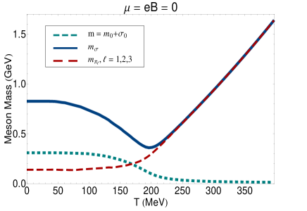
Figure 2: The $T$ dependence of $\sigma$ and $\vec{\pi}$ meson masses is demonstrated at $\mu=0$ and for a vanishing magnetic field (solid line for $m_{\sigma}$ and dashed line for $m_{\vec{\pi}}$). Comparing these curves with the $T$ dependence of the constituent quark mass $m=m_{0}+\sigma_{0}$ (dotted line) shows that a mass degeneracy between $m_{\sigma}$ and $m_{\vec{\pi}}$ occurs in the chirally restored phase $T>220$ MeV.

Comparing $T_{\mbox{\tiny{diss.}}}$ and $T_{\mbox{\tiny{Mott}}}$ for different nonvanishing $eB$ in Table 1, it seems that the crossover region is shifted to higher temperatures for increasing $eB$. In the chiral limit, where $T_{\mbox{\tiny{diss.}}}=T_{\mbox{\tiny{Mott}}}=T_{c}$, as mentioned above, this would mean that the critical temperature increases with increasing $eB$. This phenomenon is related to the magnetic catalysis of dynamical chiral symmetry breaking in the presence of external magnetic fields. Recent lattice results bali2011 show, however, a certain discrepancy with this conclusion. As it is shown in bali2011 , for certain $eB$, the critical temperature decreases with increasing $eB$. This shows that the $m$ dependence of $T_{c}$ is indeed not trivial. There are a number of attempts in the literature to resolve this disagreement inversemagnetic ; fukushima2012 , and to explain the so-called inverse magnetic catalysis rebhan2010 . Note, that, to the best of our knowledge, inverse magnetic catalysis was first observed in inagaki2003 within a two-flavor NJL model. In one of our previous papers fayazbakhsh2010 , we have also plotted the $T$-$eB$ phase diagram for different fixed chemical potential $\mu$. As it is shown in Fig. 14(a) and (b) of fayazbakhsh2010 (see also Fig. 2 in fayazbakhsh2012 ), there are some regions in $eB$ in which $T_{c}$ decreases with increasing $eB$ and the inverse magnetic catalysis occurs.

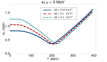
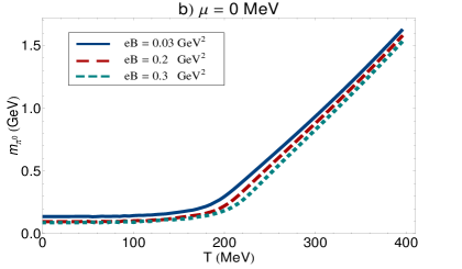
Figure 3: The $T$ dependence of $m_{\sigma}$ [panel (a)] and $m_{\pi^{0}}$ [panel (b)] is plotted for $eB=0.03,0.2,0.3$ GeV² and $\mu=0$ MeV.

In Fig. 3, the $T$ dependence of $m_{\sigma}$ [Fig. 3(a)] and $m_{\pi^{0}}$ [Fig. 3(b)] are plotted for fixed $\mu$ and $eB=0.03,0.2,0.3$ GeV². At a fixed temperature below (above) the crossover region, the $\sigma$-meson mass increases (decreases) with increasing $eB$. In contrast, $m_{\pi^{0}}$ decreases with increasing $eB$ in both symmetry broken and restored phases. The qualitative behavior of the $T$ dependence of $m_{\sigma}$ and $m_{\pi^{0}}$ for $\mu=0$ remains unchanged for zero and nonzero $eB$ (see Fig. 9 in fayazbakhsh2012 , where the $T$ dependence of $m_{\sigma}$ and $m_{\pi^{0}}$ is compared). In particular, $m_{\sigma}$ and $m_{\pi^{0}}$ are degenerate in the symmetry restored phase $T>220$ MeV.

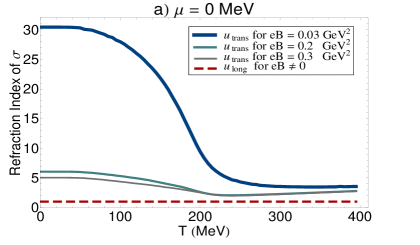
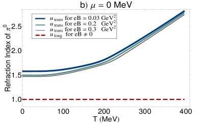
Figure 4: The $T$ dependence of the transverse and longitudinal refraction indices of $\sigma$ [panel (a)] and $\pi^{0}$ mesons [panel (b)] is plotted for various $eB$. The longitudinal refraction index of neutral mesons is equal to unity and independent of $T$ (red dashed lines). In contrast, the transverse refraction index of neutral mesons is larger than unity and decreases with increasing $eB$. For a $B$ field directed in the third direction, $u_{\mbox{\tiny{trans}}}\equiv u_{M}^{(1)}=u_{M}^{(2)}$ and $u_{\mbox{\tiny{long}}}\equiv u_{M}^{(3)}$ for $M\in\{\sigma,\pi^{0}\}$.

Let us finally consider the directional refraction indices of neutral mesons, $u_{M}^{(i)},M\in\{\sigma,\pi^{0}\}$, that appear in the energy dispersion relation (II.33). They are defined in (II.34). In what follows, we will briefly review the results appearing first in our previous paper fayazbakhsh2012 for $eB\neq 0$ and $T\neq 0$. In Fig. 4, the $T$ dependence of $u_{M}^{(i)}$ is plotted for fixed $\mu=0$ and nonvanishing $eB=0.03,0.2,0.3$ GeV². For $eB\neq 0$, the refraction indices of $\sigma$ and $\pi^{0}$ mesons in the longitudinal direction with respect to the direction of the external magnetic field turn out to be equal to unity, independent of $T$ and $\mu$ (see the red dashed lines in Figs. 4(a) and (b)]. In the transverse directions, however, the refraction indices of neutral mesons, $u_{\sigma}^{\mbox{\tiny{trans}}}$ and $u_{\pi^{0}}^{\mbox{\tiny{trans}}}$, are $T$ dependent and always larger than unity. It seems that, in the directions perpendicular to the direction of the external magnetic field, the neutral mesons move with a speed larger than the speed of light $c$. But, this is simply not true. Let us emphasize that, according to the dispersion relation (II.33), this conclusion is only valid for massless mesons, where directional group velocities coincide with $u_{M}^{(i)}$ defined in (II.34). Our mesons are, however, massive, and the fact that the transverse refraction index is larger than unity does not naturally lead to superluminal propagation. Having this in mind, the natural question is what are the consequences of $u_{\sigma}^{\mbox{\tiny{trans}}}>1$ and $u_{\pi^{0}}^{\mbox{\tiny{trans}}}>1$? One of our main motivations in this paper, is to answer this interesting question. In the next section, we will show that directional refraction indices play an important role in the low energy relations of neutral and massive pions, once we have a medium at $T\neq 0$ and/or $eB\neq 0$. But, before coming to this, let us consider again the plots in Fig. 4. As it turns out, for a fixed temperature, $u_{M}^{\mbox{\tiny{trans}}},M\in\{\sigma,\pi^{0}\}$ decrease with increasing $eB$. This effect is strongly related to the dynamics of fermions in an external magnetic field. As it is stated in miransky1995 , for very large magnetic fields, the motion of charged fermions is restricted in directions perpendicular to the magnetic field. A dimensional reduction from $3+1$ to $1+1$ dimensions occurs in the presence of very strong magnetic fields. Naively, one would expect that the properties of $\sigma$ and $\pi^{0}$ mesons are not affected by external magnetic fields, simply because they are neutral. But, as is also argued in our previous paper fayazbakhsh2012 , the way we have introduced the background magnetic field in the original Lagrangian (II.1) and the semibosonized Lagrangian (II.3) shows that the effects of the external magnetic field on neutral mesons arise mainly from its interaction with the constituent quarks of these mesonic bound states. According to this argument, the behavior of $u_{M}^{\mbox{\tiny{trans}}},M\in\{\sigma,\pi^{0}\}$ for fixed $T$ and with increasing $eB$ is a realization of the well-established dimensional reduction, appearing mainly in the lowest Landau level (LLL). Note that by increasing the magnetic field strength, the effect of higher Landau levels can be neglected, and the dynamics of fermions is solely determined by LLL, where the above-mentioned dimensional reduction occurs. This is the reason why at a fixed temperature $u_{M}^{\mbox{\tiny{trans}}},M\in\{\sigma,\pi^{0}\}$ decrease with increasing $eB$. The same property occurs at zero temperature, where the transverse velocity of neutral pions is determined within an effective chiral model in the LLL approximation fukushima2012 .

Coming back to the plots of Fig. 4, it turns out that for fixed $eB$, $u_{\sigma}^{\mbox{\tiny{trans}}}$ decreases with increasing $T$, while $u_{\pi^{0}}^{\mbox{\tiny{trans}}}$ increases with increasing $T$. The same behavior is also observed for the $T$ dependence of the mass of neutral mesons $m_{\sigma}$ and $m_{\pi^{0}}$ for a fixed $eB$ (see Fig. 2). In this paper, we do not intend to describe the nontrivial relation between $u_{M}^{\mbox{\tiny{trans}}}$ and $m_{M}$, with $M\in\{\sigma,\pi^{0}\}$. All we want to do is use the neutral pions’ directional refraction indices, and study the low energy GT and GOR relations satisfied by these neutral and massive pions. To do this, we will first modify, in the next section, the PCAC relation and prove the GT and GOR relations for $T\neq 0$ and/or $eB\neq 0$ in a model-independent way. In Sec. IV, we will then use the numerical data from the present section to prove the GT and GOR relations in a two-flavor magnetized NJL model at finite $T$. We will show, in particular, the role played by pions’ directional refraction indices in satisfying these relations.

III Directional weak decay constant of pions in random phase approximation

It is known that finite temperature and/or constant magnetic fields explicitly break the relativistic invariance. One of the main consequences of this explicit Lorentz symmetry breaking is that the massive free particles satisfy nontrivial anisotropic energy dispersion relations, including nontrivial directional energy refraction indices. As concerns the massive neutral pions, the anisotropic energy dispersion relation is given by (II.33) with $M=\pi^{0}$. Whereas at $T=eB=0$ all refraction indices are equal to unity, at $T\neq 0$ and $eB=0$, a single refraction index is defined by $u=u_{\pi^{0}}^{(1)}=u_{\pi^{0}}^{(2)}=u_{\pi^{0}}^{(3)}$, and at $T\neq 0$ and $eB\neq 0$, we have $u_{\pi^{0}}^{(1)}=u_{\pi^{0}}^{(2)}\neq u_{\pi^{0}}^{(3)}$.

It is the purpose of this paper to determine the weak decay constant of neutral pions, $f_{\pi}$, at $T\neq 0$ and $eB\neq 0$. To do this, we will generalize in this section the method presented in buballa2004 ; buballa2000 , where $f_{\pi}$ is computed at zero $T$ and $eB$ using a multiflavor NJL model. To do this, we will first review in Sec. III.1 the method presented in buballa2000 ; buballa2004 , by assuming that pions satisfy ordinary isotropic energy dispersion relations $E_{\pi}^{2}=q_{i}^{2}+m_{\pi}^{2}$. Combining the usual PCAC relation and the Feynman integral corresponding to a one-pion-to-vacuum matrix element in a random phase approximation (RPA), we arrive at the main relation leading to $f_{\pi}$ at zero $(T,\mu,eB)$. As a by-product the quark-pion coupling constant $g_{qq\pi}$ will also be defined in terms of a quark-antiquark polarization loop, in the pion channel. In buballa2004 , it is argued that in the chiral limit $m_{0}\to 0$, $f_{\pi}$ and $g_{qq\pi}$ satisfy the GT and GOR relations. We will review the method presented in buballa2000 , where these relations are proved in the leading and next-to-leading order $1/N_{c}$ expansion.

In Sec. III.2, we will then generalize the arguments in buballa2000 ; buballa2004 for free pions satisfying the anisotropic energy dispersion relation, $E_{\pi_{\ell}}^{2}=u_{\pi_{\ell}}^{(i)2}q_{i}^{2}+m_{\pi_{\ell}}^{2}$. To do this, we will first define the directional quark-pion coupling constant $g_{qq\pi_{\ell}}^{(\mu)},\mu=0,\cdots,3,$ in terms of nontrivial form factors ${\cal{F}}_{\ell\ell}^{\mu\nu}$ and refraction indices $u_{\pi_{\ell}}^{(\mu)}=(1,u_{\pi_{\ell}}^{(i)})$. We will then introduce a modified PCAC relation including ${\cal{F}}_{\ell\ell}^{\mu\nu}$, the directional refraction indices $u_{\pi_{\ell}}^{(\mu)}$ and a dimensionful proportionality factor $f_{b}$. The directional decay constant of pions, $f_{\pi_{\ell}}^{(\mu)}$, is then defined by combining ${\cal{F}}_{\ell\ell}^{\mu\nu}$ and $f_{b}$. Following the same method as in Sec. III.1, we will eventually arrive at the main relation leading to $f_{\pi_{\ell}}^{(\mu)}$. We will show that $f_{\pi_{\ell}}^{(\mu)}$ and $g_{qq\pi_{\ell}}^{(\mu)}$ satisfy modified GT and GOR relations.

III.1 Quark-pion coupling constant and pion decay constant from an isotropic energy dispersion relation

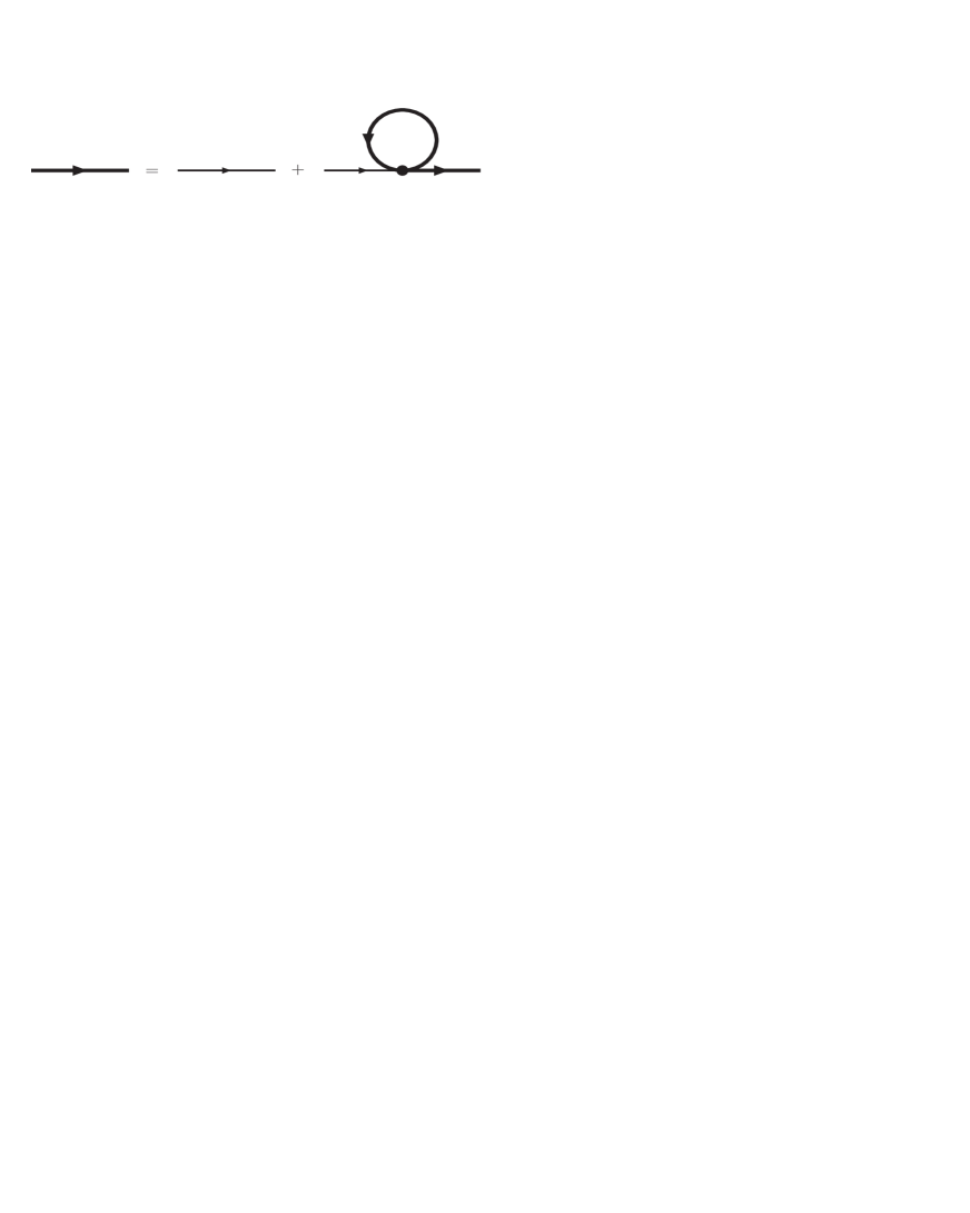
Figure 5: The Schwinger-Dyson gap equation for the quark propagator in the four-fermi NJL model in the Hartree approximation. The bare (dressed) propagator is denoted by thin (thick) lines.

Let us start with the Lagrangian density (II.1) of a two-flavor NJL model with $A_{\mu}^{\mbox{\tiny{ext.}}}=0$. As we have mentioned in the previous section, for sufficiently strong $G$, this model exhibits, in the chiral limit $m_{0}\to 0$, a dynamical mass generation. The resulting mass gap is determined via minimizing the effective (thermodynamic) potential (free energy), in a mean field approximation. Equivalently, it is given by solving the corresponding Schwinger-Dyson (SD) equation for the quark propagator. In the Hartree approximation, the constituent quark mass $m$ is given by

$$m=m_{0}+\Sigma_{H},$$ (III.1)

where $m_{0}$ is the bare quark mass and $\Sigma_{H}$ is the self-energy of quarks within the four-Fermi NJL model. In the lowest order perturbative expansion, Eq. (III.1) reduces to $m=m_{0}+\sigma_{0}$, where $\sigma_{0}=-2G\langle\bar{\psi}\psi\rangle$ is the quark condensate. This is also consistent with the diagrammatic representation of the SD equation, presented in Fig. 5. The SD relation leads to

$$m=m_{0}+\sigma_{0}\equiv m_{0}+2iG\int\frac{d^{4}p}{(2\pi)^{4}}\mbox{tr}_{sfc}S(p).$$ (III.2)

Here, $S(p)=(\gamma\cdot p-m)^{-1}$ is the dressed quark propagator. The nontrivial solution of the above integral equation leads to a mass gap $\Delta E=2m$ in the quark spectrum.

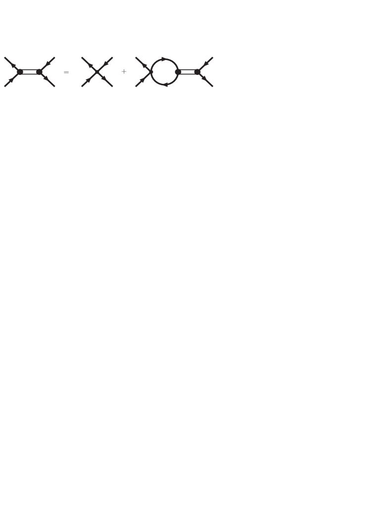
Figure 6: The Bethe-Salpeter equation for quark-antiquark scattering in RPA buballa2004 . The double lines denote the meson propagator $-(q^{2}-m_{M}^{2})^{-1}$ appearing in (III.5), and the solid lines indicate the dressed quark propagators $S(p)=(\gamma\cdot p-m)^{-1}$, including the constituent quark mass $m$. Fat vertices denote the quark-meson coupling constant defined in (III.7).

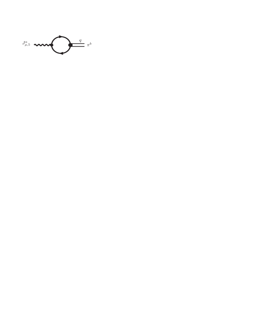
Figure 7: One-pion-to-vacuum matrix element, $\langle 0|J_{\mu,5}^{a}(0)|\pi^{b}(q)\rangle$, in RPA, leading to pion decay constant. Here, $J_{\mu,5}^{a}\equiv\bar{\psi}\gamma_{\mu}\gamma_{5}\lambda^{a}\psi$ is the axial vector current, with $\lambda^{a}\equiv\tau^{a}/2$. The solid lines are the dressed quark propagator, $S(p)=(\gamma\cdot p-m)^{-1}$, including the constituent quark mass $m$. The quark-pion coupling $g_{qq\pi_{a}}$ (fat vertex) is given in (III.7).

Similarly, mesons are described via a Bethe-Salpeter (BS) equation. In Fig. 6, the BS equation for quark-antiquark scattering is demonstrated in RPA. In this approximation, the quark-antiquark scattering matrix

$$T_{M}(q^{2})=\frac{2G}{1-2G\Pi_{M}(q^{2})},$$ (III.3)

is given in terms of the quark-antiquark polarization $\Pi_{M}(q^{2})$ in the $M\in\{\sigma,\pi\}$ channel

$$\Pi_{M}(q^{2})=i\int d^{4}x~{}\mbox{tr}_{sfc}\big{[}\Gamma_{M}S(x)\Gamma_{M}S(-x)\big{]}~{}e^{iq\cdot x}.$$

Here, $\Gamma_{\sigma}=1$ and $\Gamma_{\pi_{a}}=i\gamma_{5}\tau_{a}$. The scattering matrix $T_{M}(q^{2})$ can equivalently be written as an effective meson exchange between the external quark-antiquark legs [see the left-hand side (l.h.s.) of the relation appearing in Fig. 6],

$$T_{M}(q^{2})=-\frac{g^{2}_{qqM}}{q^{2}-m_{M}^{2}},$$ (III.5)

where $g_{qqM}$ is the quark-meson coupling constant and $m_{M}$ is the meson pole mass. Note that the denominator in (III.5) reflects the isotropic meson energy dispersion relation

$$E_{M}^{2}=q_{i}^{2}+m_{M}^{2},~{}~{}\mbox{for}~{}~{}M\in\{\sigma,\vec{\pi}\}.$$ (III.6)

Equating $T_{M}(q^{2})$ from (III.3) with (III.5) leads to the definition of the quark-meson coupling constant in terms of $\Pi_{M}(q^{2})$,

$$g_{qqM}^{-2}=\frac{d\Pi_{M}}{dq^{2}}\bigg{|}_{q^{2}=m_{M}^{2}},$$ (III.7)

as well as

$$1-2G\Pi_{M}(q^{2}=m_{M}^{2})=0,$$ (III.8)

which is equivalently given by buballa2000

$$2G\Pi_{M}(q^{2}=0)=\frac{\sigma_{0}}{m}\to 1,~{}~{}\mbox{for}~{}~{}m_{0}\to 0.$$ (III.9)

As it is argued in buballa2000 , relations (III.8) and (III.9) are consistent with Hartree approximation (III.1) as well as the RPA scheme. To determine the pion decay constant $f_{\pi}$, we consider the one-pion-to-vacuum matrix element $\langle 0|J_{\mu,5}^{a}(0)|\pi^{b}(q)\rangle$, which satisfies the usual PCAC relation

$$\langle 0|J_{\mu,5}^{a}(0)|\pi^{b}(q)\rangle=f_{\pi}q_{\mu}\delta^{ab}.$$ (III.10)

Here, $J_{\mu,5}^{a}\equiv\bar{\psi}\gamma_{\mu}\gamma_{5}\lambda^{a}\psi$ with $\lambda^{a}\equiv\tau^{a}/2$ is the axial vector current of an axial $SU(2_{f})$ global transformation. The matrix element appearing on the r.h.s. of (III.10) is demonstrated diagrammatically in Fig. 7. Note that in RPA, the quark propagator appearing in the quark-antiquark loop in Fig. 7 is the dressed quark propagator $S(p)=(\gamma\cdot p-m)^{-1}$, including the constituent quark mass $m$. Combining the PCAC relation (III.10) and the Feynman integral corresponding to the one-pion-to-vacuum amplitude demonstrated in Fig. 7, we arrive at

$$f_{\pi}q_{\mu}\delta^{ab}=g_{qq\pi}\Upsilon_{\mu}^{ab}(q),$$ (III.11)

with

$$\Upsilon_{\mu}^{ab}(q)\equiv i\int d^{4}x~{}\mbox{tr}_{sfc}\big{[}\gamma_{\mu}\gamma_{5}\lambda^{a}S(x)\gamma_{5}\tau^{b}S(-x)\big{]}e^{iq\cdot x}.$$

Contracting (III.11) with $q^{\mu}$ and using the energy dispersion relation (pion on-mass-shell condition) $q^{2}=m_{\pi}^{2}$, we arrive finally at $f_{\pi}$ in terms of $g_{qq\pi}$ and $\Upsilon_{\mu}^{ab}(q)$. As it is shown in buballa2000 , $f_{\pi}$ satisfies the GT relation

$$g_{qq\pi}f_{\pi}=m+{\cal{O}}(m_{0}^{2}),$$ (III.13)

and the GOR relation

$$m_{\pi}^{2}f_{\pi}^{2}=\frac{m_{0}\sigma_{0}}{2G}+{\cal{O}}(m_{0}^{2}),$$ (III.14)

up to second order in $m_{0}$. Let us emphasize again that the isotropic energy dispersion relation (III.6) plays an important role in proving (III.13) and (III.14) (see buballa2000 for more details). In the next section, we will show how the above relations shall be modified, when we start from a nontrivial anisotropic energy dispersion relation $q_{0}^{2}=u_{\pi_{\ell}}^{(i)2}q_{i}^{2}+m_{\pi_{\ell}}^{2}$ for free $\pi_{\ell},\ell=1,2,3$ mesons. In Sec. IV, we will use the results arising from this general consideration to determine the directional quark-pion coupling constant and decay constant for neutral pions in a hot and magnetized medium.

III.2 Directional quark-pion coupling constant and pion decay constant from an anisotropic energy dispersion relation

Let us consider the Lagrangian density

$${\cal{L}}_{\pi_{\ell}}=-\frac{1}{2}\Pi_{\ell}(x)\left(m_{\pi_{\ell}}^{2}+g^{\mu\mu}u_{\pi_{\ell}}^{(\mu)2}\partial_{\mu}^{2}\right)\Pi_{\ell}(x),$$ (III.15)

for each pion species $\pi_{\ell},\ell=1,2,3$. The above Lagrangian density is comparable to the Lagrangian of pion fields appearing in the effective action (II.15) for free mesons and leads to a nontrivial anisotropic energy dispersion relation

$$E_{\pi_{\ell}}^{2}=u_{\pi_{\ell}}^{(i)2}q_{i}^{2}+m_{\pi_{\ell}}^{2},\qquad\forall\ell=1,2,3,$$ (III.16)

similar to (II.33). In (III.15), we have introduced the “normalized” pion field $\Pi_{\ell}(x)\equiv|{\cal{F}}_{\ell\ell}^{00}|^{1/2}\pi_{\ell}(x)$, where the form factors ${\cal{F}}_{\ell\ell}^{00}$ appear in the effective action (II.15). Moreover, in analogy to (II.34) and (II.35), the mass $m_{\pi_{\ell}}$ and a four-vector for the refraction index, $u_{\pi_{\ell}}^{(\mu)}$, for each pion species $\ell=1,2,3$, are defined by the pion mass squared matrix $M_{\pi_{\ell}}^{2}$ and form factors ${\cal{F}}_{\ell\ell}^{\mu\nu}$,

$$m_{\pi_{\ell}}\equiv\bigg{|}\frac{M_{\pi_{\ell}}^{2}}{{\cal{F}}^{00}_{\ell\ell}}\bigg{|}^{1/2},\qquad u^{(\mu)}_{\pi_{\ell}}\equiv(1,u^{(i)}_{\pi_{\ell}})=\bigg{|}\frac{{\cal{F}}_{\ell\ell}^{\mu\mu}}{{\cal{F}}_{\ell\ell}^{00}}\bigg{|}^{1/2}.$$

Using ${\cal{L}}_{\pi_{\ell}}$ from (III.15), the pion propagator $D_{\pi_{\ell}}(x,y)\equiv\langle 0|T\left(\pi_{\ell}(x)\pi_{\ell}(y)\right)|0\rangle$ in the momentum space reads

$$\widetilde{D}_{\pi_{\ell}}(q)=-\frac{|{\cal{F}}_{\ell\ell}^{00}|^{-1}}{q_{0}^{2}-u_{\pi_{\ell}}^{(i)2}q_{i}^{2}-m_{\pi_{\ell}}^{2}}.$$ (III.18)

The metric $g=\mbox{diag}(1,-1,-1,-1)$. In contrast to (III.5), the denominator reflects the anisotropic pion on-mass-shell condition

$$q_{0}^{2}-u_{\pi_{\ell}}^{(i)2}q_{i}^{2}=m_{\pi_{\ell}}^{2},\qquad\forall\ell=1,2,3,$$ (III.19)

including the directional refraction indices $u_{\pi_{\ell}}^{(i)}$. The factor $|{\cal{F}}_{\ell\ell}^{00}|^{-1}$ in (III.18) arises from the normalization of pion fields, as the pion propagator can equivalently be defined by $D_{\Pi_{\ell}}(x,y)\equiv\langle 0|T\left(\Pi_{\ell}(x)\Pi_{\ell}(y)\right)|0\rangle$ with $D_{\Pi_{\ell}}=|{\cal{F}}_{\ell\ell}^{00}|D_{\pi_{\ell}}$. Using (III.18), the quark-antiquark scattering amplitude $T_{M}(q^{2})$ from (III.5) with $M=\pi_{\ell}$ is then modified as

$$T_{\pi_{\ell}}(q^{2})=-\frac{g_{qq\pi_{\ell}}^{2}|{\cal{F}}_{\ell\ell}^{00}|^{-1}}{g^{\mu\mu}u_{\pi_{\ell}}^{(\mu)2}q_{\mu}^{2}-m_{\pi_{\ell}}^{2}}.$$ (III.20)

Combining the “bare” quark-pion coupling constant $g_{qq\pi_{\ell}}$ and the normalization parameter (form factor) $|{\cal{F}}_{\ell\ell}^{00}|$ appearing also in the definition of normalized pion fields, a “normalized” coupling constant $g_{qq\Pi_{\ell}}$ is defined as

$$g_{qq\Pi_{\ell}}\equiv g_{qq\pi_{\ell}}|{\cal{F}}_{\ell\ell}^{00}|^{-1/2}.$$ (III.21)

Equating, at this stage, $T_{\pi_{\ell}}(q^{2})$ from (III.20) and the quark-antiquark scattering amplitude from (III.3) with $M=\pi_{\ell}$, we arrive first at

$$g^{\mu\mu}\frac{d\Pi_{\pi_{\ell}}(q^{2})}{dq_{\mu}^{2}}\bigg{|}_{\tilde{q}_{\pi_{\ell}}=(m_{\pi_{\ell}},\mathbf{0})}=u_{\pi_{\ell}}^{(\mu)2}|{\cal{F}}_{\ell\ell}^{00}|g_{qq\pi_{\ell}}^{-2},$$ (III.22)

$\forall\mu=0,\cdots,3$ and $\forall\ell=1,2,3$. Note that in contrast to (III.7), the expression on the l.h.s. of (III.22) is to be evaluated in the rest frame of $\ell$th pion species, i.e. in $\tilde{q}_{\pi_{\ell}}=(m_{\pi_{\ell}},{\mathbf{0}})$. Defining, at this stage, a directional quark-pion coupling constant $g_{qq\pi_{\ell}}^{(\mu)}$ by

$$\big{(}g_{qq\pi_{\ell}}^{(\mu)}(\tilde{q}_{\pi_{\ell}})\big{)}^{-2}\equiv g^{\mu\mu}\frac{d\Pi_{\pi_{\ell}}(q^{2})}{dq_{\mu}^{2}}\bigg{|}_{\tilde{q}_{\pi_{\ell}}=(m_{\pi_{\ell}},\mathbf{0})},$$ (III.23)

plugging this definition into the l.h.s. of (III.22), and using (III.2), we get

$$g^{(\mu)}_{qq\pi_{\ell}}=g_{qq\pi_{\ell}}|{\cal{F}}_{\ell\ell}^{\mu\mu}|^{-1/2}.$$ (III.24)

Similarly, the directional quark-sigma meson coupling constant is defined by

$$\big{(}g_{qq\sigma}^{(\mu)}(\tilde{q}_{\sigma})\big{)}^{-2}\equiv g^{\mu\mu}\frac{d\Pi_{\sigma}(q^{2})}{dq_{\mu}^{2}}\bigg{|}_{\tilde{q}_{\sigma}=(m_{\sigma},\mathbf{0})}.$$ (III.25)

It satisfies

$$g^{(\mu)}_{qq\sigma}=g_{qq\sigma}|{\cal{G}}^{\mu\mu}|^{-1/2}.$$ (III.26)

As it turns out, the directional coupling constant $g_{qq\pi_{\ell}}^{(\mu)}$ from (III.23) plays a crucial role in the definition of the directional weak decay constant of pions. This is determined by introducing the modified PCAC relation, which shall replace (III.10), whenever pions satisfy the anisotropic energy dispersion relation (III.16),

$$\langle 0|J_{\mu,5}^{\ell}(0)|\Pi^{m}(q)\rangle=f_{\ell}|{\cal{F}}_{\ell\ell}^{00}|^{1/2}u_{\pi_{\ell}}^{(\mu)2}q_{\mu}\delta^{\ell m},$$ (III.27)

$\forall\mu=0,\cdots,3$ and $\forall\ell,m=1,2,3$. Here, $f_{\ell}$ is an unknown dimensionful constant, which depends on $(T,\mu,eB)$, whenever they are nonvanishing. Later, we will show that, for neutral pions in the chiral limit $m_{0}\to 0$, $f_{3}=\sigma_{0}$, where $\sigma_{0}$ is the chiral condensate. For nonvanishing $m_{0}$, we get $f_{3}=m$, where $m=m_{0}+\sigma_{0}$. Note that in the chiral limit, where pions are (massless) Goldstone bosons, Eq. (III.27) leads to

$$0=\langle 0|\partial^{\mu}J_{\mu,5}^{\ell}(0)|\Pi^{m}(q)\rangle=f_{\ell}|{\cal{F}}_{\ell\ell}^{00}|^{1/2}m_{\pi_{\ell}}^{2}\delta^{\ell m},$$ (III.28)

in accordance with the Goldstone theorem. Here, the pion on-mass-shell condition (III.19) and the axial $SU(2_{f})$ invariance, $\partial^{\mu}J_{\mu,5}^{\ell}(x)=0$, are used. Using the Feynman diagram appearing in Fig. 7 for normalized pion fields, $\Pi_{\ell}$, the one-pion-to-vacuum matrix element $\langle 0|J_{\mu,5}^{\ell}(0)|\Pi^{m}(q)\rangle$ on the l.h.s. of (III.27) is given by

$$\langle 0|J_{\mu,5}^{\ell}(0)|\Pi^{m}(q)\rangle=g_{qq\Pi_{\ell}}\Upsilon_{\mu}^{\ell m}(q),$$ (III.29)

where $g_{qq\Pi_{\ell}}$ and $\Upsilon^{\ell m}(q)$ are given in (III.21) and (III.1), respectively. Relation (III.29) leads, upon using (III.21) and (III.24), as well as the modified PCAC relation (III.27), to

$$f_{\pi_{\ell}}^{(\mu)}q_{\mu}\delta^{\ell m}=g^{(\mu)}_{qq\pi_{\ell}}\Upsilon_{\mu}^{\ell m}(q),$$ (III.30)

$\forall\mu=0,\cdots,3$ and $\forall\ell,m=1,2,3$. Here, the directional pion decay constant $f_{\pi_{\ell}}^{(\mu)}$ for the $\ell$th pion species is defined by

$$f_{\pi_{\ell}}^{(\mu)}\equiv f_{\ell}|{\cal{F}}_{\ell\ell}^{\mu\mu}|^{1/2}.$$ (III.31)

In the next section, we will use (III.30) to determine $f_{\pi^{0}}^{(\mu)}$ for $\mu=0,\cdots,3$.

Similar to the previous section, the directional quark-pion coupling and decay constants satisfy the modified GT and GOR relations,

$$f_{\pi_{\ell}}^{(\mu)}g_{qq\pi_{\ell}}^{(\mu)}=m+{\cal{O}}(m_{0}^{2}),$$ (III.32)

and

$$m_{\pi_{\ell}}^{2}f_{\pi_{\ell}}^{(\mu)2}=u_{\pi_{\ell}}^{(\mu)2}\frac{m_{0}\sigma_{0}}{2G}+{\cal{O}}(m_{0}^{2}),$$ (III.33)

where $u_{\pi_{\ell}}^{(\mu)}$ is defined in (III.2). To prove these relations, we generalize the method described in buballa2000 for the case when pions satisfy nontrivial, anisotropic energy dispersion relation (III.16).

As concerns (III.32), let us consider the modified PCAC relation (III.27) and combine it with (III.29). Differentiating the l.h.s. of (III.27) and using buballa2004

$$\sum_{\mu=0}^{3}q^{\mu}\Upsilon_{\mu}^{\ell\ell}(q)=m[\Pi_{\pi_{\ell}}(q^{2})-\Pi_{\pi_{\ell}}(0)],$$ (III.34)

with the quark-antiquark polarization, $\Pi_{\pi_{\ell}}(q^{2})$ from (III.1), and $\Upsilon_{\mu}^{\ell m}=\Upsilon_{\mu}^{\ell\ell}\delta^{\ell m}$ from (III.1), we first get

$$f_{\ell}|{\cal{F}}_{\ell\ell}^{00}|m_{\pi_{\ell}}^{2}=mg_{qq\pi_{\ell}}[\Pi_{\pi_{\ell}}(q^{2})-\Pi_{\pi_{\ell}}(0)].$$ (III.35)

Expanding $\Pi_{\pi_{\ell}}(q^{2})$ on the r.h.s. of the above relation around $q=0$, and evaluating the resulting expression at $\tilde{q}_{\pi_{\ell}}$, we obtain

$$f_{\ell}|{\cal{F}}_{\ell\ell}^{00}|=mg_{qq\pi_{\ell}}\frac{d\Pi_{\pi_{\ell}}}{dq_{0}^{2}}\bigg{|}_{\tilde{q}_{\pi_{\ell}}=(m_{\pi_{\ell}},{\mathbf{0}})}+{\cal{O}}(m_{\pi_{\ell}}^{4}),$$ (III.36)

which leads, upon using (III.22) for $\mu=0$, to

$$g_{qq\pi_{\ell}}f_{\ell}=m+{\cal{O}}(m_{0}^{2}).$$ (III.37)

Plugging (III.24) as well as (III.31) into (III.37), we arrive finally at the GT relation (III.32), including directional quark-pion coupling and pion decay constants. To show the GOR relation (III.33), we use (III.8) in a slightly modified form,

$$1-2G\Pi_{\pi_{\ell}}(\tilde{q}_{\pi_{\ell}}=(m_{\pi_{\ell}},{\mathbf{0}}))=0.$$ (III.38)

This relation arises, similarly to (III.8), by equating (III.20) and (III.3) with $M=\pi_{\ell}$. Expanding the l.h.s. of (III.38) around $q^{2}=0$ and evaluating the resulting expression at $\tilde{q}_{\pi_{\ell}}=(m_{\pi_{\ell}},{\mathbf{0}})$, we get first

$$0 = 1-2G\Pi_{\pi_{\ell}}(0)-2Gm_{\pi}^{2}\frac{d\Pi_{\pi_{\ell}}(q^{2})}{dq_{0}^{2}}\bigg{|}_{\tilde{q}_{\pi_{\ell}}=(m_{\pi_{\ell}},{\mathbf{0}})}$$ (III.39)

$$+{\cal{O}}(m_{\pi_{\ell}}^{4}),$$

which yields

$$m_{\pi_{\ell}}^{2}=\frac{g_{qq\pi_{\ell}}^{2}m_{0}}{2Gm|{\cal{F}}_{\ell\ell}^{00}|}+{\cal{O}}(m_{\pi_{\ell}}^{4}).$$ (III.40)

Here, Eq. (III.9) and the definition of $g_{qq\pi_{\ell}}^{(\mu)}$ from (III.23) are used. Plugging further the GT relation (III.37) and (III.31), as well as the definition of $u_{\pi_{\ell}}^{(\mu)2}$ from (III.2) into the r.h.s. of (III.40), we arrive finally at the modified GOR relation (III.33), including $f_{\pi_{\ell}}^{(\mu)}$.

As it turns out, whereas (III.34) plays an important role in proving (III.13) and (III.14), it is not so crucial to derive (III.32) and (III.33). In the next section, we will first use the above results to derive a number of analytical expressions for the directional quark-pion coupling and decay constants for neutral pions. Using these expressions, together with the modified PCAC relation (III.27), we will then analytically prove the GT and GOR relations (III.32) and (III.33), without using (III.34). We will then verify these low energy relations for neutral pions numerically and eventually present numerical results for $g_{qq\pi^{0}}^{(\mu)}$ and $f_{\pi^{0}}^{(\mu)}$.

IV Directional quark-pion coupling and pion decay constants at finite $(T,\mu,eB)$

IV.1 Analytical results

IV.1.1 Directional quark-meson couplings for neutral mesons

Let us consider the quark-antiquark polarization $\Pi_{M}(q^{2})$ from (III.1) in the $M\in\{\sigma,\pi^{0}\}$ channel. In the presence of an external magnetic field the fermion propagators $S(x)$ appearing in (III.1) are to be replaced by Ritus propagators, $S_{Q}(x)$ from (II.1)-(II.29). Plugging (II.1) into (III.1), we arrive first at

$$\Pi_{M}(q)$$

$$=i\sum_{p,k=0}^{\infty}\int\ {\cal{D}}\tilde{p}\ {\cal{D}}\tilde{k}\int d^{4}x~{}e^{-i(\tilde{p}-\tilde{k}-q)\cdot x}\Lambda^{M}_{pk}(\bar{p},\bar{k},x_{1}),$$

where

$$\Lambda^{M}_{pk}(\bar{p},\bar{k},x_{1}) = \mbox{tr}_{sfc}\big{[}\Gamma_{M}P_{p}(x_{1})S_{Q}(\bar{p})P_{p}(0)\Gamma_{M}$$ (IV.2)

$$\times K_{k}(0)S_{Q}(\bar{k})K_{k}(x_{1})\big{]}.$$

Here, $\Gamma_{\sigma}=1$ and $\Gamma_{\pi^{0}}=i\gamma_{5}\tau^{3}$, and $\tau^{3}=\mbox{diag}(1,-1)$ is the third Pauli matrix. The momenta $\tilde{p}$ and $\bar{p}$ are defined below (II.1). In (IV.1.1), integrating first over $x_{0},x_{2},x_{3}$ and then over $p_{0},p_{2},p_{3}$ components, we arrive at the boundary conditions $p_{i}=k_{i}+q_{i}$ for $i=0,2,3$. In what follows, we will abbreviate these boundary conditions by a subscript “b.c.” Plugging $P_{p}(x_{1})$ from (II.25) into (IV.2), we arrive first at

$$\Pi_{M}(q)=i\sum_{p,k=0}^{\infty}\int\ \frac{dk_{0}dk_{3}}{(2\pi)^{3}}$$ (IV.3)

$$\times\int dk_{2}dx_{1}~{}e^{-iq_{1}x_{1}}\Lambda^{M}_{pk}(\bar{p},\bar{k},x_{1})\bigg{|}_{\mbox{\tiny{b.c.}}},$$

with

$$\Lambda^{M}_{pk}(\bar{p},\bar{k},x_{1}) = -12\sum_{q_{f}}\bigg{\{}\frac{\bar{k}.\bar{p}+\kappa_{M}m^{2}}{(\bar{p}^{2}-m^{2})(\bar{k}^{2}-m^{2})}[A^{+(0)}_{pk}\alpha^{+}_{pk}+A^{-(0)}_{pk}\alpha^{-}_{pk}]+\frac{2\bar{p}_{2}\bar{k}_{2}}{(\bar{p}^{2}-m^{2})(\bar{k}^{2}-m^{2})}A^{-(0)}_{pk}\alpha^{-}_{pk}\bigg{\}},$$ (IV.4)

where $\kappa_{\pi^{0}}=-1$ and $\kappa_{\sigma}=1$. From the decomposition

$$P_{p}(0)K_{k}(0) \equiv \alpha_{pk}^{+}(p_{2},k_{2})+is\gamma_{1}\gamma_{2}\alpha^{-}(p_{2},k_{2}),$$

$$K_{k}(x_{1})P_{p}(x_{1}) \equiv A_{pk}^{+(0)}(x_{1})+is\gamma_{1}\gamma_{2}A_{pk}^{-(0)}(x_{1}),$$

we have

$$\alpha_{pk}^{\pm(0)}(p_{2},k_{2}) \equiv \frac{1}{2}\big{[}f_{p}^{+s}(0)f_{k}^{+s}(0)$$ (IV.6)

$$\pm\Pi_{p}\Pi_{k}f_{p}^{-s}(0)f_{k}^{-s}(0)\big{]},$$

and

$$A_{pk}^{\pm(0)}(x_{1}) \equiv \frac{1}{2}\big{[}f_{p}^{+s}(x_{1})f_{k}^{+s}(x_{1})$$ (IV.7)

$$\pm\Pi_{p}\Pi_{k}f_{p}^{-s}(x_{1})f_{k}^{-s}(x_{1})\big{]}.$$

In (IV.4), the summation over $q_{f}\in\{2/3,-1/3\}$ replaces the trace in the flavor space. Moreover, we set $N_{c}=3$. In what follows, we will use $\Pi_{M}(q^{2})$ from (IV.3) to derive the directional quark-meson coupling $g_{qqM}^{(\mu)},M\in\{\sigma,\pi^{0}\}$ in the direction longitudinal, $\mu=(0,3)$, and transverse, $\mu=(1,2)$, with respect to the direction of the external magnetic field. Here, the definitions (III.23) with $\ell=3$ and (III.25), for $\big{(}g_{qqM}^{(\mu)}(\tilde{q}_{M})\big{)}^{-2},M\in\{\pi^{0},\sigma\}$ in the rest frame of mesons $\tilde{q}_{M}\equiv(m_{M},{\mathbf{0}})$, will be used.

Using $\Pi_{M}(q)$ from (IV.3) and plugging $\Lambda_{pk}^{M}(\bar{p},\bar{k},x_{1})$ from (IV.4) in

$$\big{(}g^{(\mu)}_{qqM}(\tilde{q}_{M})\big{)}^{-2}=i\sum_{p,k=0}^{\infty}\int\frac{dk_{0}dk_{3}}{(2\pi)^{3}}\int dk_{2}dx_{1}$$ (IV.8)

$$\times g^{\mu\mu}\frac{d}{dq^{2}_{\mu}}\bigg{[}e^{-iq_{1}x_{1}}\Lambda^{M}_{pk}(\bar{p},\bar{k},x_{1})\bigg{]}\bigg{|}_{\tilde{q}_{M},\mbox{\tiny{b.c.}}},$$

which arises from (III.23) and (III.25), choosing $\mu=0$, and eventually using

$$\int dk_{2}dx_{1}A_{pk}^{-(0)}\alpha_{pk}^{-}\bigg{|}_{p_{2}=k_{2}}=\frac{1}{4}|q_{f}eB|\delta_{p,k}\delta_{k,0},$$ (IV.9)

as well as

$$\int dk_{2}dx_{1}\big{[}A_{pk}^{+(0)}\alpha_{pk}^{+}+A_{pk}^{-(0)}\alpha_{pk}^{-}\big{]}\bigg{|}_{p_{2}=k_{2}}$$ (IV.10)

$$\hskip 28.45274pt=\frac{1}{2}|q_{f}eB|\alpha_{k}\delta_{p,k},$$

we arrive first at

$$\big{(}g^{(0)}_{qqM}(\tilde{q}_{M})\big{)}^{-2}=6i\sum_{q_{f}}|q_{f}eB|\sum_{k=0}^{\infty}\alpha_{k}\int_{0}^{1}dx~{}x(1-x)$$ (IV.11)

$$\times\int\frac{dk_{0}dk_{3}}{(2\pi)^{3}}\bigg{\{}\frac{3}{(\bar{k}^{2}+x(1-x)m_{M}^{2}-m^{2})^{2}}$$

$$-\frac{4\Xi_{M}(x)}{(\bar{k}^{2}+x(1-x)m_{M}^{2}-m^{2})^{3}}\bigg{\}},$$

with

$$\Xi_{\pi^{0}}(x) \equiv x(1-x)m_{\pi^{0}}^{2},$$

$$\Xi_{\sigma}(x) \equiv x(1-x)m_{\sigma}^{2}-m^{2},$$ (IV.12)

for a nonzero magnetic field and at $T=\mu=0$. In the above relations $\bar{k}^{2}={\mathbf{k}}_{\|}^{2}-2|q_{f}eB|k$ with ${\mathbf{k}}_{\|}^{2}=k_{0}^{2}-k_{3}^{2}$. To derive (IV.9) and (IV.10), we use the same technique, developed in fayazbakhsh2012 (A number of useful relations, that can be used to derive (IV.9) and (IV.10) are presented in the Appendix). At finite $(T,\mu,eB)$, we obtain

$$\big{(}g^{(0)}_{qqM}(\tilde{q}_{M})\big{)}^{-2}=-6\sum_{q_{f}}|q_{f}eB|\sum_{k=0}^{\infty}\alpha_{k}\int_{0}^{1}dxx(1-x)$$

$$\times\int\frac{dk_{3}}{(2\pi)^{2}}\bigg{\{}3{\cal{S}}^{(0)}_{2}(\omega^{M}_{k}(x))-4\Xi_{M}(x){\cal{S}}^{(0)}_{3}(\omega^{M}_{k}(x))\bigg{\}},$$

where $\Xi_{M}(x)$ is given in (IV.1.1). To introduce $(T,\mu)$, Eq. (II.30) is used. In the above relations $\omega_{k}^{M}(x),M\in\{\sigma,\pi^{0}\}$ is defined by

$$\omega_{k}^{M}(x)\equiv\big{[}k_{3}^{2}+2|q_{f}eB|k-x(1-x)m_{M}^{2}+m^{2}\big{]}^{1/2}.$$

Moreover, similar to the computation presented in fayazbakhsh2012 , we have used the functions

$${\cal{S}}_{\ell}^{(m)}(\omega)\equiv T\sum\limits_{n=-\infty}^{+\infty}\frac{(k_{0}^{2})^{m}}{(k_{0}^{2}-\omega^{2})^{\ell}},$$ (IV.15)

with $\ell\geq 1,m\geq 0$. Using

$${\cal{S}}_{1}^{(0)}(\omega)=\frac{1}{2\omega}[1-N_{f}(\omega)],$$ (IV.16)

with $N_{f}(\omega)\equiv n_{f}^{+}(\omega)+n_{f}^{-}(\omega)$ and the fermion distribution functions

$$n_{f}^{\pm}(\omega)\equiv\frac{1}{e^{\beta(\omega\mp\mu)}+1},$$ (IV.17)

the following recursion relations can be used to evaluate ${\cal{S}}_{\ell}^{(m)}(\omega)$, $\forall\ell\geq 1,m\geq 0$,

$${\cal{S}}_{\ell}^{(0)}(\omega) = \frac{1}{2(\ell-1)\omega}\frac{d{\cal{S}}_{\ell-1}^{0}(\omega)}{d\omega},\qquad\ell\geq 2,$$

$${\cal{S}}_{\ell}^{(m)}(\omega) = {\cal{S}}_{\ell-1}^{(m-1)}(\omega)+\omega^{2}{\cal{S}}_{\ell}^{(m-1)}(\omega).$$ (IV.18)

In Sec. IV.2, we will numerically evaluate the sum over Landau levels $k$ and the integration over $k_{3}$ momentum, appearing in (IV.1.1).

To determine $\big{(}g^{(1)}_{qqM}(\tilde{q}_{M})\big{)}^{-2}$, we use (IV.8) with $\mu=1$. To compute the differentiation with respect to $q_{1}^{2}$, we use the identity $\frac{df(q_{1})}{dq_{1}^{2}}|_{\tilde{q}_{M},\mbox{\tiny{b.c.}}}=\frac{1}{2}\frac{d^{2}f(q_{1})}{dq_{1}^{2}}|_{\tilde{q}_{M},\mbox{\tiny{b.c.}}}$, which is correct for $\tilde{q}_{M}=(m_{M},{\mathbf{0}})$. The integration over $k_{2}$ and $x_{1}$ can be carried out using

$$\int dk_{2}dx_{1}x_{1}A_{pk}^{\pm(0)}\alpha_{pk}^{\pm}\bigg{|}_{p_{2}=k_{2}}=0.$$ (IV.19)

We arrive first at

$$\big{(}g^{(1)}_{qqM}(\tilde{q}_{M})\big{)}^{-2}=\frac{i}{2}\sum\limits_{p,k=0}^{\infty}\int\frac{dk_{0}dk_{3}}{(2\pi)^{3}}$$ (IV.20)

$$\times\int dk_{2}dx_{1}~{}e^{-iq_{1}x_{1}}x_{1}^{2}\Lambda_{pk}^{M}(\bar{p},\bar{k},x_{1})\bigg{|}_{{\tilde{q}_{M},\mbox{\tiny{b.c.}}}},$$

for $M\in\{\sigma,\pi^{0}\}$. Plugging (IV.4) into (IV.20), and using

$$\int dk_{2}dx_{1}x_{1}^{2}\big{[}A_{pk}^{+(0)}\alpha_{pk}^{+}+A_{pk}^{-(0)}\alpha_{pk}^{-}\big{]}\bigg{|}_{p_{2}=k_{2}} = \frac{1}{2}C_{pk}^{(1)},$$

$$\int dk_{2}dx_{1}x_{1}^{2}A_{pk}^{-(0)}\alpha_{pk}^{-}\bigg{|}_{p_{2}=k_{2}} = -\frac{1}{4}C_{pk}^{(2)},$$

with $C_{pk}^{(i)},i=1,2,$ defined by

$$C_{pk}^{(1)} = \delta_{p,k}(4k+\delta_{k,0})-\Pi_{k}(2k-1)\delta_{p,k-1}$$

$$-(2k+1)\delta_{p,k+1},$$

$$C_{pk}^{(2)} = -\delta_{p,k}\delta_{k,0}+\Pi_{k}\left(2k-1-2\sqrt{k(k-1)}\right)\delta_{p,k-1}$$ (IV.22)

$$+\left(2k+1-2\sqrt{k(k+1)}\right)\delta_{p,k+1},$$

we first arrive for $B\neq 0$ and at $T=\mu=0$, at

$$\big{(}g^{(1)}_{qqM}(\tilde{q}_{M})\big{)}^{-2} = -3i\sum_{q_{f}}\sum_{p,k=0}^{\infty}\int_{0}^{1}dx\int\frac{dk_{0}dk_{3}}{(2\pi)^{3}}\bigg{\{}\frac{\big{[}{\mathbf{k}}_{\parallel}^{2}-x(1-x)m^{2}_{M}-\Delta_{pk}^{(M)}\big{]}}{\big{[}{\mathbf{k}}_{\parallel}^{2}+x(1-x)m^{2}_{M}-\Delta_{pk}\big{]}^{2}}C_{pk}^{(1)}$$ (IV.23)

$$-\frac{\bar{p}_{2}\bar{k}_{2}}{\big{[}{\mathbf{k}}_{\parallel}^{2}+x(1-x)m^{2}_{M}-\Delta_{pk}\big{]}^{2}}C^{(2)}_{pk}\bigg{\}},$$

with

$$\Delta_{pk}^{\pi^{0}} \equiv 2|q_{f}eB|\sqrt{pk}+m^{2},$$

$$\Delta_{pk}^{\sigma} \equiv 2|q_{f}eB|\sqrt{pk}-m^{2},$$

$$\Delta_{pk} \equiv 2|q_{f}eB|[(1-x)k+xp]+m^{2}.$$ (IV.24)

At finite $(T,\mu,eB)$, we therefore have

$$\big{(}g^{(1)}_{qqM}(\tilde{q}_{M})\big{)}^{-2}=3\sum_{q_{f}}\sum_{k=0}^{\infty}\int_{0}^{1}dx\int\frac{dk_{3}}{(2\pi)^{2}}\bigg{\{}(4k+\delta_{k0})\big{[}{\cal{S}}^{(0)}_{1}(\omega^{M}_{k}(x))-2\Xi_{M}(x){\cal{S}}^{(0)}_{2}(\omega^{M}_{k}(x))\big{]}$$ (IV.25)

$$-2(2k+1)\big{[}{\cal{S}}^{(0)}_{1}(\omega^{M}_{k+x}(x))-2\Xi_{M}(x){\cal{S}}^{(0)}_{2}(\omega^{M}_{k+x}(x))\big{]}+4|qeB|\left(k-x-2kx\right){\cal{S}}^{(0)}_{2}(\omega^{M}_{k+x}(x))\bigg{\}},$$

where $\Xi_{M}(x)$ and $\omega_{k}^{M}(x)$ are defined in (IV.1.1) and (IV.1.1), respectively. In the Appendix, we will present the method we have used to sum over $p$ in (IV.23) and to arrive at (IV.25).

As concerns $\big{(}g^{(2)}_{qqM}(\tilde{q}_{M})\big{)}^{-2}$, we set $\mu=2$ in (IV.8). Using $\frac{df(q_{2})}{dq_{2}^{2}}|_{\tilde{q}_{M},\mbox{\tiny{b.c.}}}=\frac{1}{2}\frac{d^{2}f(q_{2})}{dq_{2}^{2}}|_{\tilde{q}_{M},\mbox{\tiny{b.c.}}}$ and

$$\int dx_{1}dk_{2}\frac{d^{2}}{dq_{2}^{2}}\left(A_{pk}^{+(0)}\alpha_{pk}^{+}+A_{pk}^{-(0)}\alpha_{pk}^{-}\right)\bigg{|}_{p_{2}=k_{2}}=-\frac{1}{2}C_{pk}^{(1)},\qquad\int dx_{1}dk_{2}\frac{d^{2}}{dq_{2}^{2}}A_{pk}^{-(0)}\alpha_{pk}^{-}\bigg{|}_{p_{2}=k_{2}}=\frac{1}{4}C_{pk}^{(2)},$$ (IV.26)

with $C_{pk}^{(i)},i=1,2$ given in (IV.1.1), and eventually plugging these relations into the resulting expression, it turns out that

$$g^{(1)}_{qqM}(\tilde{q}_{M})=g^{(2)}_{qqM}(\tilde{q}_{M}),~{}~{}\mbox{for}~{}~{}M\in\{\sigma,\pi^{0}\}.$$ (IV.27)

At finite $(T,\mu,eB)$, the inverse squared value of $g^{(1)}_{qqM}(\tilde{q}_{M})$ is given in (IV.25). In the Appendix, we will present the necessary relations that can be used to derive (IV.26). To derive $g^{(3)}_{qqM}(\tilde{q}_{M})$, we set $\mu=3$ in (IV.8). Using (IV.9) and (IV.10), we arrive at

$$g^{(0)}_{qqM}(\tilde{q}_{M})=g^{(3)}_{qqM}(\tilde{q}_{M}),~{}~{}\mbox{for}~{}~{}M\in\{\sigma,\pi^{0}\},$$ (IV.28)

where, at finite $(T,\mu,eB)$, the inverse squared value of $g^{(0)}_{qqM}(\tilde{q}_{M})$ is given in (IV.1.1). Note that, at this stage, in the limit of $m_{\pi}\to 0$, $g_{qq\sigma}^{(\mu)}(\tilde{q}_{\sigma})$ and $g_{qq\pi^{0}}^{(\mu)}(\tilde{q}_{\pi^{0}})$, arising in (IV.1.1) and (IV.25), as well as (IV.27) and (IV.28), satisfy $g_{qq\sigma}^{(\mu)}=|{\cal{G}}^{\mu\mu}|^{-1/2}$ as well as $g_{qq\pi^{0}}^{(\mu)}=|{\cal{F}}^{\mu\mu}_{33}|^{-1/2}$. Here, the analytical expressions of ${\cal{G}}^{\mu\mu}$ and ${\cal{F}}^{\mu\mu}_{33}$ are explicitly presented in fayazbakhsh2012 . This is indeed expected from (III.24) and (III.26), which are valid for arbitrary meson masses $m_{\sigma}$ and $m_{\pi^{0}}$. This shows that $g_{qqM},M\in\{\sigma,\pi^{0}\}$ arising in (III.24) and (III.26) are, in the limit $m_{M}\to 0$, equal to unity. In Sec. IV.2, we will evaluate numerically the $k_{3}$ integration and the summation over Landau levels $k$, which appear in (IV.1.1) as well as (IV.25). We will present the $T$ dependence of directional quark-meson couplings $g_{qqM}^{(\mu)},\mu=0,\cdots,3,$ and $M\in\{\sigma,\pi^{0}\}$ at zero chemical potential and for $eB=0.03,0.2,0.3$ GeV². We will, in particular, verify (III.24) for all $T$-dependent pion masses. Moreover, we will use the data arising from these results for $g_{qqM}^{(\mu)},\mu=0,\cdots,3$, to determine the $T$ dependence of directional decay constants of neutral pions, $f_{\pi^{0}}^{(\mu)},\mu=0,\cdots,3$, at zero chemical potential and for finite and fixed magnetic fields. In what follows, we will present the analytical results for $f_{\pi^{0}}^{(\mu)},\mu=0,\cdots,3$, using (III.30) with $\ell=m=3$.

IV.1.2 Directional pion decay constant for neutral pions

Let us consider (III.30) with $\ell=3$ for neutral pions. Using the fact that $\Upsilon_{\mu}^{\ell m}(q)=\delta_{\ell m}\Upsilon_{\mu}^{\ell\ell},\forall\ell,m=1,2,3$, with $\Upsilon_{\mu}^{\ell m}$ given in (III.1), and setting $\ell=3$, we get

$$f_{\pi^{0}}^{(\mu)}q_{\mu}=g_{qq\pi^{0}}^{(\mu)}\Upsilon_{\mu}^{33}(q).$$ (IV.29)

As it turns out, Eq. (IV.29) is not appropriate to determine $f_{\pi^{0}}^{(\mu)}$ in the rest frame of neutral mesons, especially in the spatial directions. Later we will show that this is mainly because the spatial components of $\Upsilon_{\mu}^{33}(q)$ vanish in the rest frame of neutral mesons, i.e. $\Upsilon_{i}^{33}(\tilde{q}_{\pi^{0}})=0$ for $\tilde{q}_{\pi^{0}}=(m_{\pi^{0}},{\mathbf{0}})$. In what follows, after determining $\Upsilon_{\mu}^{33}(q)$ in the presence of external magnetic fields, we will present a method from which $f_{\pi^{0}}^{(\mu)}$ can be determined for all $\mu=0,\cdots,3$.

We start by plugging the Ritus propagators (II.1)-(II.29) into (III.1), to arrive at

$$\Upsilon_{\mu}^{33}(q)=\frac{i}{2}\sum\limits_{p,k=0}^{\infty}\int{\cal{D}}\tilde{p}~{}{\cal{D}}\tilde{k}$$ (IV.30)

$$\times\int d^{4}x~{}e^{-i(\tilde{p}-\tilde{k}-q)\cdot x}\Lambda_{pk}^{(\mu,3)}\left(\bar{p},\bar{k},x_{1}\right),$$

with

$$\Lambda^{(\mu,3)}_{pk}(\bar{p},\bar{k},x_{1})=\mbox{tr}_{sfc}\big{[}\gamma^{\mu}P_{p}(x_{1})S_{Q}(\bar{p})P_{p}(0)$$ (IV.31)

$$\times i\gamma_{5}\tau^{3}K_{k}(0)S_{Q}(\bar{k})K_{k}(x)i\gamma_{5}\tau^{3}\big{]}.$$

Integrating over $x_{0},x_{2},x_{3}$, and eventually over $p_{0},p_{2},p_{3}$ components, we arrive at the same boundary conditions $p_{i}=k_{i}+q_{i},i=0,2,3$, as described in the paragraph following (IV.2). Plugging $P_{p}(x_{1})$ from (II.25) into (IV.31), and using the decomposition $P_{p}(0)K_{k}(0)$, as given in (IV.1.1), and

$$K_{k}(x_{1})\gamma^{\mu}P_{p}(x_{1})$$ (IV.32)

$$=\gamma^{\mu}\big{[}(A_{pk}^{+(\mu)}(x_{1})+is\gamma_{1}\gamma_{2}A_{pk}^{-(\mu)}(x_{1})\big{]},$$

with

$$A_{pk}^{\pm(0)}=A_{pk}^{\pm(3)}$$

$$=\frac{1}{2}\big{[}f_{p}^{+s}(x_{1})f_{k}^{+s}(x_{1})\pm\Pi_{p}\Pi_{k}f_{p}^{-s}(x_{1})f_{k}^{-s}(x_{1})\big{]},$$

$$A_{pk}^{\pm(1)}=A_{pk}^{\pm(2)}$$

$$=\frac{1}{2}\big{[}\Pi_{k}f_{p}^{+s}(x_{1})f_{k}^{-s}(x_{1})\pm\Pi_{p}f_{p}^{-s}(x_{1})f_{k}^{+s}(x_{1})\big{]},$$

we arrive at

$$\Upsilon_{\mu}^{33}(q)=\frac{i}{2}\sum\limits_{p,k=0}^{\infty}\int\frac{dk_{0}dk_{3}}{(2\pi)^{3}}$$ (IV.34)

$$\times\int dk_{2}dx_{1}~{}e^{-iq_{1}\cdot x_{1}}\Lambda_{pk}^{(\mu,3)}\left(\bar{p},\bar{k},x_{1}\right)\bigg{|}_{\mbox{\tiny{b.c.}}},$$

with

$$\Lambda^{(\mu,3)}_{pk}(\bar{p},\bar{k},x_{1})=12m\sum_{q_{f}}\bigg{\{}\frac{(\bar{p}-\bar{k})_{\mu}{\cal{N}}_{pk}^{(\mu)}-isg^{\mu 1}\big{[}\bar{k}_{2}{\cal{M}}_{pk}^{+(\mu)}+\bar{p}_{2}{\cal{M}}_{pk}^{-(\mu)}\big{]}+2g^{\mu 2}\bar{p}_{2}{\cal{P}}_{pk}^{(\mu)}}{(\bar{p}^{2}-m^{2})(\bar{k}^{2}-m^{2})}\bigg{\}},$$ (IV.35)

and

$${\cal{N}}_{pk}^{(\mu)}\equiv A^{+(\mu)}_{pk}\alpha^{+}_{pk}+A^{-(\mu)}_{pk}\alpha^{-}_{pk},\qquad{\cal{M}}_{pk}^{\pm(\mu)}\equiv A_{pk}^{+(\mu)}\alpha_{pk}^{-}\pm A_{pk}^{-(\mu)}\alpha_{pk}^{+},\qquad{\cal{P}}_{pk}^{(\mu)}=\alpha^{-}_{pk}A^{-(\mu)}_{pk}.$$ (IV.36)

Using (IV.10) as well as

$$\int dk_{2}dx_{1}A_{pk}^{\pm(1)}\alpha_{pk}^{\pm}\bigg{|}_{p_{2}=k_{2}}=0,\qquad\int dk_{2}dx_{1}A_{pk}^{\pm(1)}\alpha_{pk}^{\mp}\bigg{|}_{p_{2}=k_{2}}=0,$$ (IV.37)

and performing the integration over $k_{2}$ and $x_{1}$ in (IV.34) for $q=\tilde{q}_{\pi^{0}}$, we get

$$\Upsilon_{i}^{33}(\tilde{q}_{\pi^{0}})=0,\qquad\mbox{for}\qquad i=1,2,3.$$ (IV.38)

Thus, in order to determine $f_{\pi^{0}}^{(\mu)}$ from (IV.29), especially in the spatial directions, we have to expand the r.h.s. of (IV.29) around $\tilde{q}_{\pi^{0}}$, and then evaluate both sides at $\tilde{q}_{\pi^{0}}$. Keeping in mind that $g_{qq\pi^{0}}^{(\mu)}$, appearing on the r.h.s. of (IV.29) and defined in (III.23), depends, in general, on $q$, we obtain

$$f_{\pi^{0}}^{(0)} = m_{\pi^{0}}^{-1}g_{qq\pi^{0}}^{(0)}(\tilde{q}_{\pi^{0}})\Upsilon_{0}^{33}(\tilde{q}_{\pi^{0}}),$$ (IV.39)

$$f_{\pi^{0}}^{(i)} = g_{qq\pi^{0}}(\tilde{q}_{\pi^{0}})\frac{d}{dq_{i}}\Upsilon_{i}^{33}(\tilde{q}_{\pi^{0}}),$$ (IV.40)

for $i=1,2,3$. In what follows, Eqs. (IV.39) and (IV.40) will be used to determine the analytical expressions for $f_{\pi^{0}}^{(\mu)},\mu=0,\cdots,3$.

Setting $\mu=0$ in (IV.34) with $\Lambda_{pk}^{(\mu,3)}$ given in (IV.35), and using (IV.10) to evaluate the integration over $k_{2}$ and $x_{1}$, $f_{\pi^{0}}^{(0)}$ from (IV.39) reads

$$f^{(0)}_{\pi^{0}}=3img^{(0)}_{qq\pi^{0}}(\tilde{q}_{\pi^{0}})\sum_{k=0}^{\infty}\alpha_{k}\sum_{q_{f}}|q_{f}eB|$$

$$\times\int_{0}^{1}dx\int\frac{dk_{0}dk_{3}}{(2\pi)^{3}}\frac{1}{\big{[}\bar{k}^{2}+x(1-x)m_{\pi^{0}}^{2}-m^{2}\big{]}^{2}},$$

for nonzero $eB$ and vanishing $T$ and $\mu$, as well as

$$f^{(0)}_{\pi^{0}}=-3m\ g^{(0)}_{qq\pi^{0}}\sum_{q_{f}}|q_{f}eB|\sum_{k=0}^{\infty}\alpha_{k}$$ (IV.42)

$$\times\int_{0}^{1}dx\int\frac{dk_{3}}{(2\pi)^{2}}S^{(0)}_{2}(\omega^{\pi^{0}}_{k}(x)),$$

at finite $(T,\mu,eB)$. Here, ${\cal{S}}_{2}^{(0)}(\omega_{k}^{\pi^{0}}(x))$ with $\omega_{k}^{\pi^{0}}(x)$ from (IV.1.1) is defined in (IV.15) and can be evaluated using the recursion relations in (IV.1.1).

Plugging $i=1$ into (IV.40), we arrive first at

$$f_{\pi^{0}}^{(1)}=6img_{qq\pi^{0}}^{(1)}(\tilde{q}_{\pi^{0}})\sum_{p,k=0}^{\infty}\sum_{q_{f}}s\int\frac{dk_{0}dk_{3}}{(2\pi)^{3}}$$

$$\times\int dk_{2}dx_{1}\frac{[\bar{k}_{2}{x_{1}\cal{M}}_{pk}^{+(1)}+\bar{p}_{2}x_{1}{\cal{M}}_{pk}^{-(1)}]}{(\bar{p}^{2}-m^{2})(\bar{k}^{2}-m^{2})}\bigg{|}_{\tilde{q}_{\pi^{0}},\mbox{\tiny{b.c.}}},$$

where ${\cal{M}}_{pk}^{\pm(1)}$ are defined in (IV.36) with $\mu=1$. The integrations over $k_{2}$ and $x_{1}$ can be performed using

$$\int dk_{2}dx_{1}x_{1}A_{pk}^{\pm(1)}\alpha_{pk}^{\mp}=-\frac{\sqrt{|q_{f}eB|}}{4\sqrt{2}}$$ (IV.44)

$$\times\big{[}\Pi_{k}\delta_{p,k-1}(\sqrt{k}\mp\sqrt{k-1})$$

$$\pm\Pi_{k+1}\delta_{p,k+1}(\sqrt{k+1}\mp\sqrt{k})\big{]}.$$

After plugging (IV.44) into (IV.1.2) and summing over $p$, by making use of the method described in the Appendix, we arrive, after some work, at

$$f_{\pi^{0}}^{(1)}=6img_{qq\pi^{0}}^{(1)}(\tilde{q}_{\pi^{0}})\sum_{k=0}^{\infty}\sum_{q_{f}}|q_{f}eB|\int\frac{dk_{0}dk_{3}}{(2\pi)^{3}}$$

$$\times\frac{1}{[{\mathbf{k}}_{\|}^{2}+x(1-x)m_{\pi^{0}}^{2}-m^{2}-2|q_{f}eB|(k+x)]^{2}},$$

for nonvanishing $eB$ and at zero $(T,\mu)$. At finite $(T,\mu,eB)$, we therefore get

$$f_{\pi^{0}}^{(1)}=-6mg_{qq\pi^{0}}^{(1)}(\tilde{q}_{\pi^{0}})\sum\limits_{k=0}^{\infty}\sum_{q_{f}}|q_{f}eB|$$ (IV.46)

$$\times\int_{0}^{1}dx\int\frac{dk_{3}}{(2\pi)^{2}}{\cal{S}}_{2}^{(0)}(\omega_{k+x}^{\pi^{0}}(x)).$$

To determine $f_{\pi^{0}}^{(2)}$, we use (IV.40) with $i=2$. Plugging (IV.34)-(IV.35) into the resulting expression, using

$$\int dk_{2}dx_{1}\alpha_{pk}^{\pm}\frac{d}{dk_{2}}A_{pk}^{\pm(1)}\bigg{|}_{p_{2}=k_{2}}=0,$$ (IV.47)

as well as

$$\int dk_{2}dx_{1}A_{pk}^{\pm(1)}\frac{d}{dk_{2}}\alpha_{pk}^{\pm}\bigg{|}_{p_{2}=k_{2}}=\frac{s|q_{f}eB|}{4\sqrt{2}}$$

$$\times\big{[}\Pi_{k}\delta_{p,k-1}(\sqrt{k}\pm\sqrt{k-1})\mp\delta_{p,k+1}(\sqrt{k+1}\pm\sqrt{k})\big{]},$$

and eventually summing over $p$, using the method presented in the Appendix, we arrive, after some algebraic computations, at

$$f_{\pi^{0}}^{(2)}=f_{\pi^{0}}^{(1)},$$ (IV.49)

with $f_{\pi^{0}}^{(1)}$ given in (IV.1.2) for nonvanishing $eB$ and at zero $(T,\mu)$, and in (IV.46) for finite $(T,\mu,eB)$. Finally, setting $i=3$ in (IV.40), and using (IV.10) to perform the integration over $k_{2}$ and $x_{1}$, keeping in mind that, according to (IV.1.2), $A_{pk}^{\pm(3)}=A_{pk}^{\pm(0)}$, we arrive easily at

$$f_{\pi^{0}}^{(3)}=f_{\pi^{0}}^{(0)},$$ (IV.50)

with $f_{\pi^{0}}^{(0)}$ given in (IV.1.2) for nonvanishing $eB$ and at zero $(T,\mu)$, and in (IV.42) for finite $(T,\mu,eB)$. Using (IV.42) and (IV.46) as well as (IV.49) and (IV.50) for $f_{\pi^{0}}^{(\mu)}$, it can easily be checked that, in the limit $m_{\pi^{0}}\to 0$, $f_{\pi^{0}}^{(\mu)}$ satisfies $f_{\pi^{0}}^{(\mu)}=m|{\cal{F}}_{33}^{\mu\mu}|^{1/2}$, with ${\cal{F}}_{33}^{\mu\mu}$ given explicitly in fayazbakhsh2012 . Comparing this relation with the definition of $f_{\pi^{0}}^{(\mu)}$ from (III.31) with $\ell=3$, it turns out that the dimensionful constant $f_{3}$, appearing originally in the Ansatz (III.27), is, in the limit of vanishing $m_{\pi^{0}}$, equal to the constituent mass $m$. In Sec. IV.2, after numerically computing $f_{\pi^{0}}^{(\mu)}$ from (IV.42) and (IV.46), we will determine the coefficient $f_{3}$ using (III.31) and compare its $T$ dependence for fixed $\mu$ and $eB$ with the $T$ dependence of the constituent mass $m$ for arbitrary $T$-dependent $m_{\pi^{0}}$. But, before doing this, let us analytically verify the modified GT relation (III.32). In Sec. III.2, we have used (III.36) to prove (III.32). For zero magnetic fields, the explicit form of $\Upsilon_{\mu}^{\ell m}$ as a function of the fermion propagator $S(p)$ is to be used to verify (III.35). In the presence of magnetic fields, however, where nontrivial Ritus propagators $S_{Q}(p)$ from (II.1) are to be used to determine $\Upsilon_{\mu}^{\ell m}$, relation (III.35) cannot be directly proved. To show the GT relation for neutral magnetized pions, we use, instead, the analytical results of $\Upsilon_{0}^{(33)}$ and $(g_{qq\pi^{0}}^{(0)})^{-2}$ and verify first the following relation:

$$\Upsilon_{0}^{(33)}(\tilde{q}_{\pi^{0}})=mm_{\pi^{0}}(g_{qq\pi^{0}}^{(0)})^{-2}+{\cal{O}}(m_{\pi^{0}}^{2}).$$ (IV.51)

Combining further (III.27) and (III.29) for $\ell=m=3$, and evaluating the resulting expression

$$g_{qq\Pi^{0}}\Upsilon_{\mu}^{33}(q)=f_{3}|{\cal{F}}_{33}^{00}|^{1/2}u_{\pi^{0}}^{(\mu)2}q_{\mu},$$

on the pion mass shell, i.e., for $q=\tilde{q}_{\pi^{0}}=(m_{\pi^{0}},{\mathbf{0}})$, we obtain

$$g_{qq\pi^{0}}\Upsilon_{0}^{(33)}(\tilde{q}_{\pi^{0}})=f_{3}|{\cal{F}}_{33}^{00}|m_{\pi^{0}},$$ (IV.52)

which leads, together with (III.24) and (IV.51), to

$$g_{qq\pi^{0}}f_{3}=m+{\cal{O}}(m_{\pi^{0}}),$$ (IV.53)

and eventually, upon using (III.24) and (III.31), to the GT relation

$$g_{qq\pi^{0}}^{(\mu)}f_{\pi^{0}}^{(\mu)}=m+{\cal{O}}(m_{\pi^{0}}),$$ (IV.54)

for neutral pions. Note that (IV.53) is the same as (III.37) with $\ell=3$. In Sec. III.2, we have shown how the GOR relation (III.33) for neutral pions,

$$m_{\pi^{0}}^{2}f_{\pi^{0}}^{(\mu)2}=u_{\pi^{0}}^{(\mu)2}\frac{m_{0}\sigma_{0}}{2G}+{\cal{O}}(m_{0}^{2}),$$ (IV.55)

can be derived from (IV.53) and (III.38). As concerns the proof of (IV.51), we use (IV.34) and (IV.35) with $\mu=0$. Using (IV.10) to perform the integration over $k_{3}$ and $x_{1}$, we arrive at

$$\Upsilon_{0}^{(33)}(\tilde{q}_{\pi^{0}}) = 3imm_{\pi^{0}}\sum\limits_{k=0}^{\infty}\alpha_{k}\sum_{q_{f}}\int\frac{dk_{0}dk_{3}}{(2\pi)^{3}}$$ (IV.56)

$$\times\frac{1}{[(k_{0}+m_{\pi^{0}})^{2}-k_{3}^{2}-2|q_{f}eB|k-m^{2}]}$$

$$\times\frac{1}{[{\mathbf{k}}_{\|}^{2}-2|q_{f}eB|-m^{2}]}.$$

Expanding the r.h.s. of this relation in orders of $m_{\pi^{0}}$, we get

$$\Upsilon_{0}^{(33)}(\tilde{q}_{\pi^{0}}) = -3mm_{\pi^{0}}\sum\limits_{k=0}^{\infty}\alpha_{k}\sum\limits_{q_{f}}\int\frac{dk_{3}}{(2\pi)^{2}}~{}{\cal{S}}_{2}^{(0)}(\omega_{k})$$ (IV.57)

$$+{\cal{O}}(m_{\pi^{0}}^{2}),$$

at finite $(T,\mu,eB)$. Here, ${\cal{S}}_{2}^{(0)}(\omega_{k})$ is defined in (IV.15) and $\omega_{k}^{2}=k_{3}^{2}+m^{2}+2|q_{f}eB|k$. On the other hand, let us consider $(g_{qqM}^{(0)}(\tilde{q}_{M}))^{-2}$ from (IV.1.1). For $M=\pi^{0}$, it consists of two terms. Neglecting the second term proportional to $m_{\pi^{0}}^{2}$, expanding ${\cal{S}}_{2}^{(0)}(\omega_{k}^{\pi^{0}}(x))$, appearing in the first term around $m_{\pi^{0}}=0$, and eventually integrating the resulting expression over the Feynman parameter $x$, we get

$$(g_{qq\pi^{0}}^{(0)}(\tilde{q}_{\pi^{0}}))^{-2} = -3\sum\limits_{k=0}^{\infty}\alpha_{k}\sum\limits_{q_{f}}\int\frac{dk_{3}}{(2\pi)^{2}}~{}{\cal{S}}_{2}^{(0)}(\omega_{k})$$ (IV.58)

$$+{\cal{O}}(m_{\pi^{0}}^{2}),$$

which, together with (IV.57), leads to (IV.51). This proves the GT and GOR relations in the limit $m_{\pi^{0}}\to 0$. In what follows, we will numerically verify, among others, these relations for arbitrary pion mass at finite $(T,\mu,eB)$.

IV.2 Numerical results

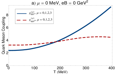
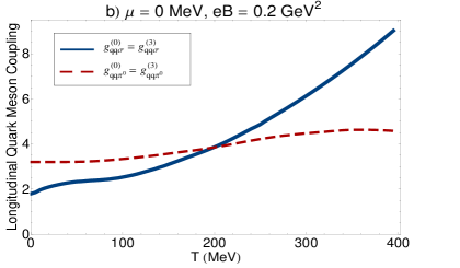
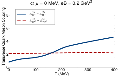
Figure 8: The $T$ dependence of directional quark-meson couplings is demonstrated for $eB=0$ [panel (a)] and $eB=0.2$ GeV² [panels (b) and (c)]. Solid blue curves are directional quark-sigma couplings $g_{qq\sigma}^{(\mu)}$, and the dashed red curves are the directional quark-pion couplings $g_{qq\pi^{0}}^{(\mu)}$. In contrast to $eB\neq 0$, for $eB=0$, there is no difference between the quark-meson couplings in longitudinal and transverse directions with respect to the direction of the external magnetic field $eB$.

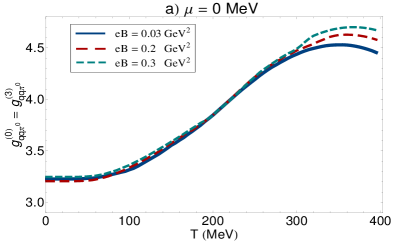
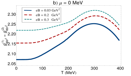
Figure 9: The $T$ dependence of directional quark-pion couplings $g_{qq\pi^{0}}^{(\mu)}$ are demonstrated for vanishing chemical potential and $eB=0.03,0.2,0.3$ GeV². In panels (a) and (b), the longitudinal coupling $g_{qq\pi^{0}}^{(0)}=g_{qq\pi^{0}}^{(3)}$ and transverse coupling $g_{qq\pi^{0}}^{(1)}=g_{qq\pi^{0}}^{(2)}$ are plotted, respectively. The couplings show different behaviors by increasing the strength of the magnetic field $eB$ at fixed $T$, and similar behaviors before and after the transition temperature $T_{c}\sim 200$ MeV.

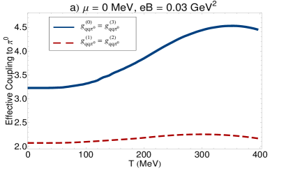
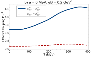
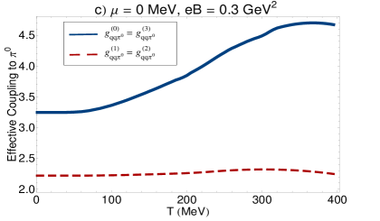
Figure 10: Longitudinal (blue solid curves) and transverse (red dashed curves) quark-pion couplings, $g_{qq\pi^{0}}^{(0)}=g_{qq\pi^{0}}^{(3)}$ and $g_{qq\pi^{0}}^{(1)}=g_{qq\pi^{0}}^{(2)}$, are compared in the interval $T\in[0,400]$ MeV for vanishing chemical potential and various $eB=0.03$ GeV² [panel (a)], $eB=0.2$ GeV² [panel (b)] and $eB=0.3$ GeV² [panel (c)]. As it turns out, the longitudinal coupling is always greater than the transverse coupling.

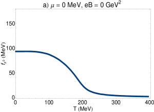
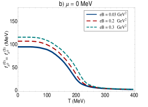
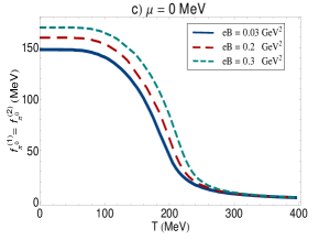
Figure 11: [Panel (a)] The $T$ dependence of $f_{\pi^{0}}$ for vanishing chemical potential and magnetic field. Panels (b) and (c): The $T$ dependence of longitudinal [panel (b)] and transverse [panel (c)] decay constants of neutral pions are plotted for zero chemical potential and nonvanishing $eB=0.03,0.2,0.3$ GeV².

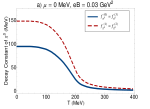
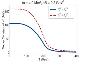
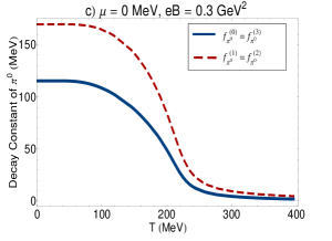
Figure 12: The $T$ dependence of longitudinal (blue solid curves) and transverse (red dashed curves) decay constants of neutral pions, $f_{\pi^{0}}^{(0)}$ and $f_{\pi^{0}}^{(1)}$, are compared for vanishing chemical potential and nonvanishing $eB=0.03,0.2,0.3$ GeV². As it turns out, $f_{\pi^{0}}^{(0)}<f_{\pi^{0}}^{(1)}$.

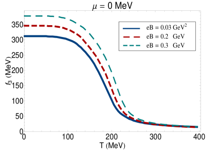
Figure 13: The $T$ dependence of $f_{3}$ appearing in the PCAC relation (III.27). Here, $f_{3}$ is determined using $f_{3}=f_{\pi^{0}}^{(0)}|{\cal{F}}_{33}^{00}|^{-1/2}$ from (III.31) with $\ell=3$. Comparing these results with the corresponding data from the $T$ dependence of the constituent quark mass $m$, it turns out that $f_{3}=m$ for an arbitrary value of $m_{\pi^{0}}$.

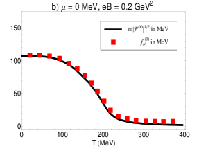
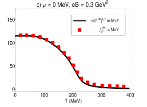
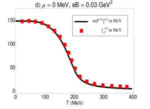
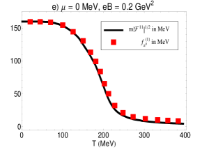
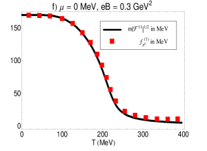
Figure 14: The $T$ dependence of $f_{\pi^{0}}^{(\mu)}$ (red squares) is compared with the $T$ dependence of $m|{\cal{F}}_{33}^{\mu\mu}|^{1/2}$ (black solid lines) for longitudinal $\mu=0,3$ [panels (a)-(c)] and transverse directions $\mu=1,2$ [panels (d)-(e)]. Together with the definition $f_{\pi^{0}}^{(\mu)}=f_{3}|{\cal{F}}_{33}^{\mu\mu}|^{1/2}$ from (III.31) with $\ell=3$, we obtain $f_{3}=m$, as expected also from the comparison of the data of $f_{3}$ in Fig. 13 and the constituent quark mass $m=m_{0}+\sigma_{0}$ in Fig. 1.

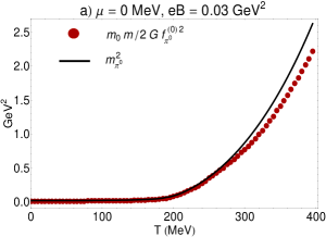
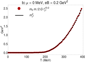
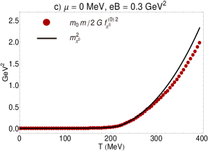
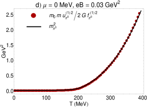
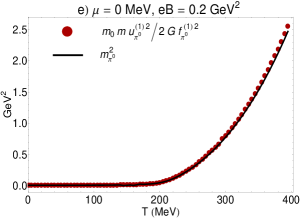
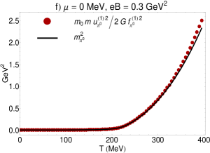
Figure 15: To verify the relation (IV.61), suggested by the GOR relation (IV.55), the $T$ dependence of $m_{\pi^{0}}^{2}$ (black solid lines) is compared with $\frac{m_{0}m}{2Gf_{\pi^{0}}^{(0)2}}$ (red dots) [panels (a)-(c)] and with $u_{\pi^{0}}^{(1)2}\frac{m_{0}m}{2Gf_{\pi^{0}}^{(1)2}}$ (red dots) [panels (d)-(f)]. Relation (IV.61) seems to be exact, especially at temperatures below the critical temperature and for small $eB$.

In the previous section, we determined analytically the directional neutral mesons coupling and decay constants, $g_{qqM}^{(\mu)},M\in\{\sigma,\pi^{0}\}$ and $f_{\pi^{0}}^{(\mu)}$, at finite $(T,\mu,eB)$ up to an integration over $k_{3}$ momentum and a summation over discrete Landau levels. Using these analytical results, it is possible to prove the GT and GOR relations in the limit of $m_{\pi^{0}}\to 0$. In the present section, we will numerically determine the $T$ dependence of $g_{qqM}^{(\mu)},M\in\{\sigma,\pi^{0}\}$ and $f_{\pi^{0}}^{(\mu)}$ for zero chemical potential and finite $eB=0.03,0.2,0.3$ GeV². We will compare $g_{qqM}^{(0)}$ with $g_{qqM}^{(1)}$, which corresponds to quark-meson couplings in the longitudinal and transverse directions with respect to the direction of the external magnetic field. We then present the results for the $T$ dependence of $f_{\pi^{0}}^{(\mu)}$ for vanishing chemical potential and fixed $eB$, and will compare $f_{\pi^{0}}^{(0)}$ with $f_{\pi^{0}}^{(1)}$. Using these numerical results, and the results from our previous paper fayazbakhsh2012 , we will numerically determine the dimensionful constant $f_{3}$, appearing in the definition (III.31) with $\ell=3$. We will show that, for arbitrary $m_{\pi^{0}}$, it is given by the constituent quark mass $m$. Finally, a numerical verification of the GOR relation will be presented.

Let us start by fixing the parameters of our specific model, $\Lambda,G$ and $m_{0}$. As in fayazbakhsh2010 ; fayazbakhsh2012 , we have used

$$\Lambda=0.6643 \mbox{GeV}, \qquad G=4.668~{}\mbox{GeV}^{2},$$

$$\qquad m_{0}=5 \mbox{MeV}.$$ (IV.59)

The UV momentum cutoff $\Lambda$ is necessary to perform the $k_{3}$ integrations in the results for $g_{qqM}^{(\mu)},M\in\{\sigma,\pi^{0}\}$ and $f_{\pi^{0}}^{(\mu)}$ from previous sections. It is also used to determine the upper limit $c$ for the summation over Landau levels. We will fix $c$ by building the ratio $\lfloor\frac{\Lambda^{2}}{|q_{f}eB|}\rfloor\equiv c$, where $\lfloor z\rfloor$ is the greatest integer less than or equal to $z$. To perform the momentum integrations over ${\mathbf{k}}$ and $k_{3}$, we use, as in fayazbakhsh2010 ; fayazbakhsh2012 , smooth cutoff functions

$$f_{\Lambda,0} = \frac{1}{1+\exp\left(\frac{|{\mathbf{k}}|-\Lambda}{A}\right)},$$

$$f_{\Lambda,B}^{k} = \frac{1}{1+\exp\left(\frac{\sqrt{k_{3}^{2}+2|q_{f}eB|k}-\Lambda}{A}\right)},$$ (IV.60)

which correspond to integrals with vanishing and nonvanishing magnetic fields. In $f_{\Lambda,B}^{k}$, the upper index $k$ labels the Landau levels. In (IV.2), $A$ is a free parameter, that determines the sharpness of the cutoff. It is fixed to be $A=0.05\Lambda$, with $\Lambda$ from (IV.2). As we have also mentioned in Sec. II, fixing the free parameters of the model as in (IV.2), the constituent mass $m$ at zero $(T,\mu,eB)$ turns out to be $m\sim 308$ MeV, as expected. Moreover, the pion mass and decay constant for vanishing $(T,\mu,eB)$ are given by $m_{\pi}\sim 139.6$ MeV and $f_{\pi}=93.35$ MeV, respectively. These values are expected from the phenomenology of a two-flavor NJL model buballa2004 . We will limit all our numerical computations in this section in the interval $T\in[0,400]$ MeV for vanishing $\mu$ and $eB=0,0.03,0.2,0.3$ GeV². As we have shown in fayazbakhsh2010 ; fayazbakhsh2012 , in this interval the chiral symmetry of the theory is broken and the quark condensate $\sigma_{0}\sim\langle\bar{\psi}\psi\rangle$, appearing in $m=m_{0}+\sigma_{0}$, plays the role of the order parameter of the transition from a chirally broken to a chirally symmetric phase.

In Figs. 8(a)-(c), we have plotted the $T$ dependence of the directional quark-meson coupling $g_{qq\sigma}^{(\mu)}$ (solid blue curves) and $g_{qq\pi^{0}}^{(\mu)}$ (red dashed curves) for $eB=0$ [Fig. 8(a)] and $eB=0.2$ GeV² [Figs. 8(b) and 8(c)]. Whereas for $eB=0$, there is no difference between $g_{qqM}^{(\mu)},M\in\{\sigma,\pi^{0}\}$ for different directions $\mu=0,\cdots,3$, for $eB\neq 0$, the longitudinal and transverse quark-meson couplings for $\sigma$ and $\pi^{0}$ are different [compare the solid blue and dashed red curves in Figs. 8(b) and 8(c)]. At certain temperature $T_{\mbox{\tiny{cross}}}$, the two curves cross, i.e., $g_{qq\sigma}^{(\mu)}$ becomes equal to $g_{qq\pi^{0}}^{(\mu)}$. For $T<T_{\mbox{\tiny{cross}}}$, $g_{qq\sigma}^{(\mu)}<g_{qq\pi^{0}}^{(\mu)}$ and for $T>T_{\mbox{\tiny{cross}}}$, $g_{qq\sigma}^{(\mu)}>g_{qq\pi^{0}}^{(\mu)}$. Moreover, as it turns out, for $eB=0$, $T_{\mbox{\tiny{diss.}}}<T_{\mbox{\tiny{cross}}}<T_{\mbox{\tiny{Mott}}}$. For $eB\neq 0$, however, we have to separate the longitudinal and transverse cases. Whereas for longitudinal couplings, we have $T_{\mbox{\tiny{diss.}}}<T_{\mbox{\tiny{cross}}}<T_{\mbox{\tiny{Mott}}}$, for transverse couplings, we get $T_{\mbox{\tiny{cross}}}<T_{\mbox{\tiny{diss.}}}<T_{\mbox{\tiny{Mott}}}$. Whether this temperature is of certain relevance, in particular, in the scattering length and the total cross section of meson-meson scattering, where the thermodynamic properties of quark-meson couplings play an important role is under investigation.

In Fig. 9, the $T$ dependence of directional quark-pion couplings, $g_{qq\pi^{0}}^{(\mu)}$, is plotted for vanishing chemical potential and various $eB=0,0.03,0.2,0.3$ GeV². The longitudinal quark-pion coupling $g_{qq\pi^{0}}^{(0)}=g_{qq\pi^{0}}^{(3)}$ from (IV.1.1) with $M=\pi^{0}$ is plotted in Fig. 9(a), and the transverse quark-pion coupling $g_{qq\pi^{0}}^{(1)}=g_{qq\pi^{0}}^{(2)}$ from (IV.25) with $M=\pi^{0}$ is plotted in Fig. 9(b). Whereas the behavior of longitudinal and transverse couplings is different by increasing the strength of the external magnetic field for a fixed temperature, it turns out to be similar when we increase the temperature from $T=0$ to $T=400$ MeV. An inflection point arises in directional quark-pion coupling constants around the critical temperature $T\sim 200$ MeV. Comparing the longitudinal and transverse quark-pion couplings in Fig. 10, it turns out that $g_{qq\pi^{0}}^{(0)}>g_{qq\pi^{0}}^{(1)}$ in the interval $T\in[0,400]$ MeV and for fixed chemical potential and magnetic fields. This is a direct consequence of the fact that the transverse refraction index of pions is larger than unity: As we have seen in Fig. 4, $u_{\pi^{0}}^{(1)}=u_{\pi^{0}}^{(2)}>1$. Using $g_{qq\pi^{0}}^{(\mu)}=g_{qq\pi^{0}}|{\cal{F}}_{33}^{\mu\mu}|^{-1/2}$ from (III.24) with $\ell=3$, and $u_{\pi^{0}}^{(\mu)}=\big{|}{{\cal{F}}_{33}^{\mu\mu}/{\cal{F}}_{33}^{00}}\big{|}^{1/2}$ from (III.2), we will get $g_{qq\pi^{0}}^{(0)}=g_{qq\pi^{0}}|{\cal{F}}_{33}^{00}|^{-1/2}$ as well as $g_{qq\pi^{0}}^{(1)}=g_{qq\pi^{0}}^{(0)}/u_{\pi^{0}}^{(1)}$. For $u_{\pi^{0}}^{(1)}>1$, it turns out that $g_{qq\pi^{0}}^{(0)}>g_{qq\pi^{0}}^{(1)}$, as is observed in Fig. 10.

Let us now consider the longitudinal and transverse pion decay constants, $f_{\pi^{0}}^{(0)}=f_{\pi^{0}}^{(3)}$ and $f_{\pi^{0}}^{(1)}=f_{\pi^{0}}^{(2)}$ from (IV.42) and (IV.46), respectively. In Fig. 11(a), the $T$ dependence of $f_{\pi^{0}}$ is plotted for vanishing chemical potential and magnetic fields. In Figs. 11(b) and 11(c), the $T$ dependence of longitudinal and transverse decay constants of neutral pions, $f_{\pi^{0}}^{(0)}$ and $f_{\pi^{0}}^{(1)}$, is plotted for zero chemical potential and nonvanishing magnetic fields $eB=0.03,0.2,0.3$ GeV². In both cases, $f_{\pi^{0}}^{(\mu)}$ is large below the critical temperature and decreases with increasing temperature. At a fixed temperature, the directional pion decay constants increase as the strength of the magnetic field increases. In Figs. 12(a)-12(c), we have compared the $T$ dependence of the longitudinal and transverse decay constants for $\mu=0$ and $eB=0.03,0.2,0.3$ GeV². As it turns out, $f_{\pi^{0}}^{(0)}<f_{\pi^{0}}^{(1)}$. This behavior is again related to $u_{\pi^{0}}^{(1)}>1$ from Fig. 4: Using the definition $f_{\pi^{0}}^{(\mu)}=f_{3}|{\cal{F}}_{33}^{\mu\mu}|^{1/2}$ from (III.31) with $\ell=3$, and $u_{\pi^{0}}^{(\mu)}=\big{|}{{\cal{F}}_{33}^{\mu\mu}/{\cal{F}}_{33}^{00}}\big{|}^{1/2}$ from (III.2), it turns out that $f_{\pi^{0}}^{(0)}=f_{3}|{\cal{F}}_{33}^{00}|^{1/2}$ and $f_{\pi^{0}}^{(1)}=f_{\pi^{0}}^{(0)}u_{\pi^{0}}^{(1)}$. For $u_{\pi^{0}}^{(1)}>1$, we have therefore $f_{\pi^{0}}^{(0)}<f_{\pi^{0}}^{(1)}$, as observed in Fig. 12. Note that combining $g_{qq\pi^{0}}^{(1)}=g_{qq\pi^{0}}^{(0)}/u_{\pi^{0}}^{(1)}$ and $f_{\pi^{0}}^{(1)}=f_{\pi^{0}}^{(0)}u_{\pi^{0}}^{(1)}$ yields the GT relation (III.32).

Using the corresponding data of $f_{\pi^{0}}^{(\mu)}$ and the definition of directional decay constant $f_{\pi^{0}}^{(\mu)}$ from (III.31) with $\ell=3$, it is possible to determine the $T$ dependence of $f_{3}$ defined by $f_{\pi^{0}}^{(\mu)}=f_{3}|{\cal{F}}_{33}^{\mu\mu}|^{1/2}$. To do this, we have also used the data corresponding to the $T$ dependence of ${\cal{F}}_{33}^{\mu\mu}$ from our previous paper fayazbakhsh2012 . In Fig. 13, we have presented the $T$ dependence of $f_{3}$ for vanishing chemical potential and various $eB=0.03,0.2,0.3$ GeV². Comparing these results with the corresponding data from the $T$ dependence of the constituent quark mass $m$, it turns out that $f_{3}=m$ for an arbitrary value of $m_{\pi^{0}}$. According to our arguments from fayazbakhsh2012 , for a fixed $T$ and $\mu$, the constituent quark mass increases with increasing strength of the magnetic field (see also Fig. 1). This is because of the phenomenon of magnetic catalysis klimenko1992 ; miransky1995 . We conclude therefore that the behavior of longitudinal and transverse pion decay constants in external magnetic fields at fixed temperature and chemical potential is mainly affected by this phenomenon.

Note that another way to verify $f_{3}=m$ is to compare the $T$ dependence of $f_{\pi^{0}}^{(\mu)}$ on the l.h.s. of the relation $f_{\pi^{0}}^{(\mu)}=m|{\cal{F}}_{33}^{\mu\mu}|^{1/2}$ with the $T$ dependence of $m|{\cal{F}}_{33}^{\mu\mu}|^{1/2}$ on the r.h.s. of this relation for longitudinal directions $\mu=0,3$ [Figs. 14(a)-14(c)], and transverse directions $\mu=1,2$ [Figs. 14(d)-14(f)]. The red squares denote the data for $f_{\pi^{0}}^{(\mu)},\mu=0,1$ and the black solid lines the combination $m|{\cal{F}}^{00}|^{1/2}$ for longitudinal $\mu=0,3$ and $m|{\cal{F}}^{11}|^{1/2}$ for transverse $\mu=1,2$ directions.

Let us now consider the GOR relation (IV.55) for neutral pions. In Sec. IV.1, we have analytically proved the GOR relation (IV.55) in the limit of vanishing $m_{\pi^{0}}$. In Fig. 15, however, we have compared the $T$ dependence of the expression $u_{\pi^{0}}^{(\mu)2}\frac{m_{0}m}{2Gf_{\pi^{0}}^{(\mu)}}$ (red dots) with the $T$ dependence of $m_{\pi^{0}}^{2}$ (black solid lines) for any value of $m_{\pi^{0}}$ for various $eB=0.03,0.2,0.3$ GeV². In Figs. 15(a)-15(c), we present the data for longitudinal directions, i.e. for $\mu=0$ with $u_{\pi^{0}}^{(0)}=u_{\pi^{0}}^{(3)}=1$ [see Fig. 4(b) for the longitudinal refraction index of neutral pions], and in Figs 15(d)-15(f) the data for transverse directions are presented. Note that, according to Fig. 4 fayazbakhsh2012 , the transverse refraction index of neutral pions is larger than unity. As it is shown in Fig. 15, the relation

$$m_{\pi^{0}}^{2}=u_{\pi^{0}}^{(\mu)2}\frac{m_{0}m}{2Gf_{\pi^{0}}^{(\mu)}},$$ (IV.61)

seems to be exact in the interval below the critical temperature. As we have explained in fayazbakhsh2012 , the critical temperature is defined by the temperature from which the neutral pion mass starts to increase. The deviations of the expression on the r.h.s. of (IV.61) from $m_{\pi^{0}}^{2}$ on the l.h.s. of this relation depend on $eB$ and $T$.

V Summary and Conclusions

Uniform magnetic fields affect the properties of mesons in a hot and dense quark matter. In our previous paper fayazbakhsh2012 , we systematically studied these effects on the pole and screening mass as well as the refraction index of pions. In the present paper, we continued with exploring the effect of constant magnetic fields on the pion weak decay constant. One of our first observations was that external magnetic fields break the isospin symmetry of pions, insofar as charged and neutral pions behave differently in the external magnetic fields. In contrast to the studies performed in andersen2011-pions ; anderson2012-2 , where chiral perturbation theory is used to study the effect of constant magnetic fields on the properties of charged pions, we focused on the properties of neutral pions in external magnetic fields.

In this paper, following the same method as in our previous paper fayazbakhsh2012 , we used an appropriate derivative expansion up to second order and derived the effective action of a two-flavor bosonized NJL model at finite $(T,\mu,eB)$ in this approximation. The resulting effective action is given as a functional of $\sigma$ and $\pi^{0}$ mesons and includes a kinetic and a potential part. To derive the mass and refraction indices of neutral mesons, we focused, in particular, on the nontrivial kinetic part of the effective action, including nontrivial form factors. They were evaluated in fayazbakhsh2012 using the method presented in Sec. II. As it turns out, they play an essential role in defining the pole and screening mass as well as the directional refraction indices of neutral pions. As concerns the pions’ refraction index, it turns out that in the presence of a constant magnetic field, aligned in a fixed direction, the refraction indices of neutral pions parallel to the direction of the external magnetic field and in the plane perpendicular to this direction are different. Within our approximation, where the contributions of pion-pion interactions are neglected, and at $T\neq 0$ and $eB\neq 0$, the longitudinal refraction index is unity for all nonvanishing $T$ and $eB$, while the transverse refraction index is larger than unity. This is in contrast to the case $T=0$ and $eB=0$, where the refraction index for neutral pions in all spatial directions is equal to unity. This is also in contrast to the case $T\neq 0$ and $eB=0$, where all spatial refraction indices are equal to and smaller than unity pisarski1996 ; son2000 ; ayala2002 . One of the possibilities to improve the results in this paper is to include pion self-interaction terms in the original Lagrangian for pions and to study the $T$ dependence of directional refraction indices in the longitudinal and transverse directions in that setup.

Our central analytical result in this paper is presented in Sec. III. In Sec. III.1, we briefly reviewed the method introduced in buballa2004 and derived the weak decay constant of pions at zero $T$ and $eB$. In this case, the pions satisfy an ordinary isotropic energy dispersion relation $E_{\pi}^{2}={\mathbf{q}}^{2}+m_{\pi}^{2}$, and the weak decay constant $f_{\pi}$ is given by combining the ordinary PCAC relation and the Feynman integral corresponding to a one-pion-to-vacuum amplitude. As a by-product, the momentum-dependent quark-pion coupling constant $g_{qq\pi}(q)$ is also defined. Our starting point in Sec. III.2, however, was an anisotropic energy dispersion relation, $E_{\pi}^{2}=u_{\pi}^{(i)2}q_{i}^{2}+m_{\pi}^{2}$, including directional refraction indices $u_{\pi}^{(i)},i=1,2,3$. Note that, according to the above arguments, the case of nonvanishing magnetic field and/or finite temperature can be viewed only as special cases of the general assumption of Sec. III.2. Introducing a modified PCAC relation with nontrivial four-vector $u_{\pi_{a}}^{(\mu)}=(1,u^{(i)}_{\pi_{a}})$, as given in (III.27), and following the same arguments as in Sec. III.1, we derived the modified GT and GOR relations, (III.32) and (III.33), including the directional pion weak decay constant $f_{\pi^{0}}^{(\mu)}$ and the directional quark-pion coupling constant $g_{qq\pi^{0}}^{(\mu)}$.

In Sec. IV, we then used the results arising from the general treatment presented in Sec. III.2 and determined $g_{qq\pi^{0}}^{(\mu)}$ as well as $f_{\pi^{0}}^{(\mu)}$ at finite $T$ and $eB$ first analytically in Sec. IV.1, and then numerically in Sec. IV.2. As it turns out, the longitudinal and transverse quark-pion coupling and weak decay constants satisfy $g_{qq\pi^{0}}^{(0)}=g_{qq\pi^{0}}^{(3)}\neq g_{qq\pi^{0}}^{(1)}=g_{qq\pi^{0}}^{(2)}$ and $f_{\pi^{0}}^{(0)}=f_{\pi^{0}}^{(3)}\neq f_{\pi^{0}}^{(1)}=f_{\pi^{0}}^{(2)}$. We determined numerically their $T$ dependence for various $eB$. We showed that, whereas $g_{qq\pi^{0}}^{(0)}>g_{qq\pi^{0}}^{(1)}$, we have $f_{\pi^{0}}^{(0)}<f_{\pi^{0}}^{(1)}$. This is a direct consequence of the fact that $1=u_{\pi^{0}}^{(0)}<u_{\pi^{0}}^{(1)}$, as it is shown in Fig. 4. Moreover, for a fixed $\mu$ and $eB$, whereas the mass of neutral pions increases with increasing $T$ [see Fig. 3(b)], the directional decay constants of pions decrease with $T$. At fixed $\mu$ and $T$, they increase with increasing strength of the external magnetic field (see Fig. 11). As concerns the behavior of pions, directional decay constants $f_{\pi^{0}}^{(\mu)},\mu=0,\cdots,3$ near the chiral transition point $T_{c}$, it turns out, that, independent of the direction, they are almost constant but large at $T\ll T_{c}$, start to decrease at $T\simeq T_{c}$ and remain constant but very small at $T\gg T_{c}$. Moreover, the slope of this decrease as a function of $T$ depends on the strength of the external magnetic field. The behavior of $g_{qq\pi^{0}}^{(\mu)}$ and $f_{\pi^{0}}^{(\mu)}$ in the external magnetic field and at finite $T$ is strongly related to the behavior of the constituent quark mass $m$ at finite $T$ and $eB$. This relationship is reflected in the low energy relations of neutral pions, the GT and GOR relations. We not only derived these relations analytically in Sec. IV.1, but also verified them numerically in Sec. IV.2. The behavior of the constituent quark mass $m$ at finite $T$ and $eB$ was discussed extensively in our previous paper fayazbakhsh2012 . Comparing Figs. 1 and 11(a)-11(c), it turns out that $m$ and $f_{\pi^{0}}^{(\mu)}$ have similar $T$ dependence for a fixed $eB$. The phenomenon of magnetic catalysis is reflected in the fact that at fixed $\mu$ and $T$, they both increase with increasing $eB$. As we have shown in Sec. III, $f_{\pi^{0}}^{(\mu)}$ and $m$ are proportional, and the proportionality factor is, according to the GT relation (III.32), $1/g_{qq\pi^{0}}^{(\mu)}$. Let us finally note that our results can be improved by improving the approximation we have used to determine the kinetic coefficients to higher order derivative expansion, or by making use of the functional renormalization group method, which was recently used in skokov2012 .

Appendix: Useful relations

In this appendix, we present a number of useful relations leading to the analytical results presented in Sec. IV. Let us start with the orthonormality relations of $f_{p}^{\pm s}$ appearing in (II.27),

$$\int dx_{1}\ f^{+s}_{p}(x)f^{+s}_{k}(x)\bigg{|}_{p_{2}=k_{2}} = \delta_{pk},$$

$$\int dx_{1}\ x_{1}\ f^{+s}_{p}(x)f^{+s}_{k}(x)\bigg{|}_{p_{2}=k_{2}} = \ell_{B}\bigg{\{}\Pi_{k}C_{k}\delta_{p,k-1}$$

$$+\Pi_{k+1}C_{k+1}\delta_{p,k+1}+s\ell_{B}k_{2}\delta_{p,k}\bigg{\}},$$

$$\int dx_{1}\ x_{1}^{2}\ f^{+s}_{p}(x)f^{+s}_{k}(x)\bigg{|}_{p_{2}=k_{2}}$$ (A.1)

$$=\ell_{B}^{2}\bigg{\{}(2C_{2k+1}^{2}+\ell_{B}^{2}k_{2}^{2})\delta_{pk}+\Pi_{k}\Pi_{k-1}C_{k}C_{k-1}\delta_{p,k-2}$$

$$+C_{k+1}C_{k+2}\delta_{p,k+2}+2\Pi_{k}C_{k}s\ell_{B}k_{2}\delta_{p,k-1}$$

$$+2\Pi_{k+1}C_{k+1}s\ell_{B}k_{2}\delta_{p,k+1}\bigg{\}},$$

and

$$\int dk_{2}\ f^{+s}_{p}(0)f^{+s}_{k}(0)\bigg{|}_{p_{2}=k_{2}} = \frac{\delta_{pk}}{\ell_{B}^{2}},$$

$$\int dk_{2}\ k_{2}\ f^{+s}_{p}(0)f^{+s}_{k}(0)\bigg{|}_{p_{2}=k_{2}} = -\frac{s}{\ell_{B}^{3}}\bigg{\{}C_{k+1}\delta_{p,k+1}$$

$$+\Pi_{k}C_{k}\delta_{p,k-1}\bigg{\}},$$

$$\int dk_{2}\ k_{2}^{2}\ f^{+s}_{p}(0)f^{+s}_{k}(0)\bigg{|}_{p_{2}=k_{2}} = \frac{1}{\ell_{B}^{4}}\bigg{\{}2C_{2k+1}^{2}\delta_{pk}$$

$$+\Pi_{k}\Pi_{k-1}C_{k}C_{k-1}\delta_{p,k-2}+C_{k+1}C_{k+2}\delta_{p,k+2}\bigg{\}}.$$

Here, $C_{k}\equiv\sqrt{\frac{k}{2}}$ and $\ell_{B}\equiv\frac{1}{\sqrt{|q_{f}eB|}}$. To derive these relations, we have used

$$x_{1}f_{p}^{+s}(x) = \ell_{B}\bigg{\{}\Pi_{p+1}C_{p+1}f_{p+1}^{+s}(x)+\Pi_{p}C_{p}f_{p-1}^{+s}(x)$$

$$+s\ell_{B}p_{2}f_{p}^{+s}(x)\bigg{\}},$$

$$p_{2}f_{p}^{+s}(x) = -\frac{s}{\ell_{B}}\bigg{\{}\Pi_{p+1}C_{p+1}f_{p+1}^{+s}(x)$$ (A.3)

$$+\Pi_{p}C_{p}f_{p-1}^{+s}(0)\bigg{\}}.$$

Apart from (IV.44), we have

$$\int dx_{1}dk_{2}x_{1}A_{pk}^{+(1)}\alpha_{pk}^{+}=\frac{1}{4\ell_{B}}\bigg{\{}2\Pi_{k}C_{k}\alpha_{k}$$ (A.4)

$$-\Pi_{k}\delta_{p,k-1}\left(C_{k}+C_{k-1}\right)$$

$$-\Pi_{k+1}\delta_{p,k+1}\left(C_{k+1}-C_{k}\right)\bigg{\}},$$

as well as

$$\int dx_{1}dk_{2}x_{1}A_{pk}^{-(1)}\alpha_{pk}^{-}$$ (A.5)

$$=-\frac{1}{4\ell_{B}}\bigg{\{}\Pi_{k}\delta_{p,k-1}\left(C_{k}-C_{k-1}\right)$$

$$-\Pi_{k+1}\delta_{p,k+1}\left(C_{k+1}-C_{k}\right)\bigg{\}},$$

which can be used to derive (IV.1.2) as well as

$$\int dx_{1}dk_{2}\frac{d}{dk_{2}}\bigg{[}\alpha_{pk}^{+}A_{pk}^{+(1)}+\alpha_{pk}^{-}A_{pk}^{-(1)}\bigg{]}\bigg{|}_{p_{2}=k_{2}}$$ (A.6)

$$= -\frac{s}{2\ell_{B}^{2}}\big{[}\Pi_{k}\delta_{p,k-1}+\delta_{p,k-1}\big{]}.$$

Similarly, we have

$$\int dx_{1}dk_{2}\frac{d}{dk_{2}}\bigg{[}\alpha_{pk}^{+}A_{pk}^{+(0)}+\alpha_{pk}^{-}A_{pk}^{-(0)}\bigg{]}\bigg{|}_{p_{2}=k_{2}}$$ (A.7)

$$= -\frac{s}{2\ell_{B}^{2}}\big{[}\Pi_{k}\delta_{p,k-1}+\delta_{p,k-1}\big{]}.$$

Finally, we present the method leading to $g_{qq\pi^{0}}^{(1)}$ from (IV.25) and to $f_{\pi^{0}}^{(1)}$ from (IV.1.2). The relations leading to (IV.25) and (IV.49) have the following general structure:

$$I \equiv \sum\limits_{p,k=0}^{\infty}\int_{0}^{1}dxf(p,k,x)$$ (A.8)

$$\times\big{[}\Pi_{k}\delta_{p,k-1}F(p,k)+\delta_{p,k+1}G(p,k)\big{]}.$$

The aim is to show

$$I=\sum\limits_{k=0}\int_{0}^{1}dxf(k+1,k,x)\big{[}F(k,k)+G(k+1,k)\big{]}.$$

Starting from (A.8) and summing over $p$, we arrive first at

$$I = \sum\limits_{k=0}^{\infty}\int_{0}^{1}dx\big{[}\Pi_{k}f(k-1,k,x)F(k-1,k)$$ (A.10)

$$+f(k+1,k,x)G(k+1,k)\big{]}.$$

Changing the variables in the first term and using the property of $f(p,k,x)$

$$f(k,k+1,x)=f(k,k+1,1-x),$$

we arrive at

$$I = \sum\limits_{k=0}^{\infty}\int_{0}^{1}dx\big{[}f(k,k+1,1-x)F(k)$$

$$+f(k+1,k,x)G(k+1)\big{]}.$$

Then using the symmetry property

$$\int_{0}^{1}dxf(k+1,k,1-x)=\int_{0}^{1}dxf(k+1,k,x),$$

we arrive at (Appendix: Useful relations). In all our examples in Sec. IV, $f(p,k,x)$ has the general form

$$f(p,k,x)=\frac{A+B\sqrt{pk}}{[C+x(1-x)m^{2}+D(px+k(1-x))]^{2}}.$$

References

- (1) J. W. Holt, N. Kaiser and W. Weise, Nuclear chiral dynamics and thermodynamics, arXiv:1304.6350 [nucl-th].
- (2) S. -i. Nam and H. -C. Kim, Pion weak decay constant at finite density from the instanton vacuum, Phys. Lett. B 666, 324 (2008), arXiv:0805.0060 [hep-ph].
- (3) M. Buballa, NJL model analysis of quark matter at large density, Phys. Rept. 407, 205 (2005), arXiv:hep-ph/0402234.
- (4) T. Hell, S. Rossner, M. Cristoforetti and W. Weise, Thermodynamics of a three-flavor nonlocal Polyakov-Nambu-Jona-Lasinio model, Phys. Rev. D 81, 074034 (2010), arXiv:0911.3510 [hep-ph].
- (5) K. G. Klimenko, Three-dimensional Gross-Neveu model at nonzero temperature and in an external magnetic field, Z. Phys. C 54, 323 (1992).
- (6) V. P. Gusynin, V. A. Miransky, I. A. Shovkovy, Dimensional reduction and catalysis of dynamical symmetry breaking by a magnetic field, Nucl. Phys. B 462, 249 (1996), arXiv:hep-ph/9509320.
- (7) D. E. Kharzeev, K. Landsteiner, A. Schmitt and H. -U. Yee, “Strongly interacting matter in magnetic fields”: an overview, Lect. Notes Phys. 871, 1 (2013), arXiv:1211.6245 [hep-ph].
- (8) R. Gatto and M. Ruggieri, Quark matter in a strong magnetic background, Lect. Notes Phys. 871, 87 (2013), arXiv:1207.3190 [hep-ph]. I. A. Shovkovy, Magnetic catalysis: A review, Lect. Notes Phys. 871, 13 (2013), arXiv:1207.5081 [hep-ph]. F. Preis, A. Rebhan and A. Schmitt, Inverse magnetic catalysis in field theory and gauge-gravity duality, Lect. Notes Phys. 871, 51 (2013), arXiv:1208.0536 [hep-ph]. E. J. Ferrer and V. de la Incera, Magnetism in dense quark matter, Lect. Notes Phys. 871, 399 (2013), arXiv:1208.5179 [nucl-th]. E. S. Fraga, Thermal chiral and deconfining transitions in the presence of a magnetic background, Lect. Notes Phys. 871, 121 (2013), arXiv:1208.0917 [hep-ph]. K. Fukushima, Views of the chiral magnetic effect, Lect. Notes Phys. 871, 241 (2013), arXiv:1209.5064 [hep-ph]. M. A. Andreichikov, B. O. Kerbikov, V. D. Orlovsky and Y. A. Simonov, Meson spectrum in strong magnetic fields, Phys. Rev. D 87, 094029 (2013), arXiv:1304.2533 [hep-ph]. A. Ayala, L. A. Hernandez, J. Lopez, A. J. Mizher, J. C. Rojas and C. Villavicencio, Phase diagram for charged scalars in a magnetic field at finite temperature, arXiv:1305.1583 [hep-ph]. C. S. Machado, F. S. Navarra, E. G. de Oliveira, J. Noronha and M. Strickland, Heavy quarkonium production in a strong magnetic field, Phys. Rev. D 88, 034009 (2013), arXiv:1305.3308 [hep-ph].
- (9) S. Fayazbakhsh, S. Sadeghian and N. Sadooghi, Properties of neutral mesons in a hot and magnetized quark matter, Phys. Rev. D 86, 085042 (2012), arXiv:1206.6051 [hep-ph].
- (10) N. O. Agasian and I. A. Shushpanov, Gell-Mann-Oakes-Renner relation in a magnetic field at finite temperature, JHEP 0110, 006 (2001), arXiv:hep-ph/0107128.
- (11) I. V. Selyuzhenkov [STAR Collaboration], Global polarization and parity violation study in Au + Au collisions, Rom. Rep. Phys. 58, 049 (2006), arXiv:nucl-ex/0510069. D. E. Kharzeev, L. D. McLerran and H. J. Warringa, The effects of topological charge change in heavy ion collisions: ’Event by event P and CP violation’, Nucl. Phys. A 803, 227 (2008), arXiv:0711.0950 [hep-ph]. A. Bzdak and V. Skokov, Event-by-event fluctuations of magnetic and electric fields in heavy ion collisions, Phys. Lett. B 710, 171 (2012), arXiv:1111.1949 [hep-ph].
- (12) V. Skokov, A. Y. Illarionov and V. Toneev, Estimate of the magnetic field strength in heavy-ion collisions, Int. J. Mod. Phys. A 24, 5925 (2009), arXiv:0907.1396 [nucl-th]. K. Tuchin, Time and space dependence of electromagnetic field in relativistic heavy-ion collisions, Phys. Rev. C 88, 024911 (2013), arXiv:1305.5806 [hep-ph].
- (13) E. V. Shuryak, Physics of the pion liquid, Phys. Rev. D 42, 1764 (1990).
- (14) D. T. Son and M. A. Stephanov, Pion propagation near the QCD chiral phase transition, Phys. Rev. Lett. 88, 202302 (2002), arXiv:hep-ph/0111100. D. T. Son and M. A. Stephanov, Real time pion propagation in finite temperature QCD, Phys. Rev. D 66, 076011 (2002), arXiv:hep-ph/0204226.
- (15) A. Ayala, P. Amore and A. Aranda, Pion dispersion relation at finite density and temperature, Phys. Rev. C 66, 045205 (2002), arXiv:hep-ph/0207081.
- (16) R. D. Pisarski and M. Tytgat, Propagation of cool pions, Phys. Rev. D 54, 2989 (1996), arXiv:hep-ph/9604404; ibid., Cool pions move at less than the speed of light, in Proceedings of the Continuous Advances in QCD, Minneapolis, MI, 196, (1996), arXiv:hep-ph/9606459; ibid. Scattering of soft, cool pions, Phys. Rev. Lett. 78, 3622 (1997), arXiv:hep-ph/9611206.
- (17) D. Toublan, Pion dynamics at finite temperature, Phys. Rev. D 56, 5629 (1997), arXiv:hep-ph/9706273. U. G. Meissner, J. A. Oller and A. Wirzba, In-medium chiral perturbation theory beyond the mean field approximation, Annals Phys. 297 (2002) 27, arXiv:nucl-th/0109026.
- (18) N. Bilic and H. Nikolic, Superluminal pions in a hadronic fluid, Phys. Rev. D 68, 085008 (2003), arXiv:hep-ph/0301275. J. Alexandre, J. Ellis and N. E. Mavromatos, On the Possibility of Superluminal Neutrino Propagation, Phys. Lett. B 706, 456 (2012), arXiv:1109.6296 [hep-ph].
- (19) V. I. Ritus, Radiative corrections in quantum electrodynamics with intense fields and their analytical properties, Ann. Phys. 69, (1972) 555.
- (20) K. Fukushima, D. E. Kharzeev and H. J. Warringa, Electric-current susceptibility and the chiral magnetic effect, Nucl. Phys. A 836, 311 (2010), arXiv:0912.2961 [hep-ph].
- (21) N. Sadooghi and F. Taghinavaz, Local electric current correlation function in an exponentially decaying magnetic field, Phys. Rev. D 85, 125035 (2012), arXiv:1203.5634 [hep-ph].
- (22) K. Heckmann, M. Buballa and J. Wambach, Chiral restoration effects on the shear viscosity of a pion gas, Prog. Part. Nucl. Phys. 67, 348 (2012), arXiv:1202.0724 [hep-ph].
- (23) I. A. Shushpanov and A. V. Smilga, Quark condensate in a magnetic field, Phys. Lett. B 402, 351 (1997), arXiv:hep-ph/9703201.
- (24) E. Quack, P. Zhuang, Y. Kalinovsky, S. P. Klevansky and J. Hufner, - scattering lengths at finite temperature, Phys. Lett. B 348, 1 (1995) , hep-ph/9410243.
- (25) G. S. Bali, F. Bruckmann, G. Endrodi, Z. Fodor, S. D. Katz, S. Krieg, A. Schafer and K. K. Szabo, The QCD phase diagram for external magnetic fields, JHEP 1202, 044 (2012), arXiv:1111.4956 [hep-lat]; ibid. PoS LATTICE 2011, 192 (2011), arXiv:1111.5155 [hep-lat]. G. S. Bali, F. Bruckmann, M. Constantinou, M. Costa, G. Endrodi, Z. Fodor, S. D. Katz, S. Krieg, H. Panagopoulos and A. Schafer, Thermodynamic properties of QCD in external magnetic fields, PoS ConfinementX , 198 (2012), arXiv:1301.5826 [hep-lat]. M. D’Elia, Lattice QCD simulations in external background fields, Lect. Notes Phys. 871, 181 (2013), arXiv:1209.0374 [hep-lat].
- (26) E. S. Fraga and L. F. Palhares, Deconfinement in the presence of a strong magnetic background: An exercise within the MIT bag model, Phys. Rev. D 86, 016008 (2012), arXiv:1201.5881 [hep-ph]. J. O. Andersen and A. A. Cruz, Two-color QCD in a strong magnetic field: The role of the Polyakov loop, Phys. Rev. D 88, 025016 (2013), arXiv:1211.7293 [hep-ph]. F. Bruckmann, G. Endrodi and T. G. Kovacs, Inverse magnetic catalysis and the Polyakov loop, JHEP 1304, 112 (2013), arXiv:1303.3972 [hep-lat]. N. Callebaut and D. Dudal, On the transition temperature(s) of magnetized two-flavour holographic QCD, Phys. Rev. D 87, 106002 (2013), arXiv:1303.5674 [hep-th]. J. Chao, P. Chu and M. Huang, Inverse magnetic catalysis induced by sphalerons, arXiv:1305.1100 [hep-ph]. W. -C. Syu, D. -S. Lee and C. N. Leung, External magnetic fields and the chiral phase transition in QED at nonzero chemical potential, arXiv:1307.8222 [hep-ph].
- (27) K. Fukushima and Y. Hidaka, Magnetic catalysis vs magnetic inhibition, Phys. Rev. Lett. 110, 031601 (2013), arXiv:1209.1319 [hep-ph].
- (28) F. Preis, A. Rebhan and A. Schmitt, Inverse magnetic catalysis in dense holographic matter, JHEP 1103, 033 (2011), arXiv:1012.4785 [hep-th].
- (29) T. Inagaki, D. Kimura and T. Murata, Four fermion interaction model in a constant magnetic field at finite temperature and chemical potential, Prog. Theor. Phys. 111, 371 (2004), hep-ph/0312005.
- (30) Sh. Fayazbakhsh and N. Sadooghi, Phase diagram of hot magnetized two-flavor color superconducting quark matter, Phys. Rev. D 83, 025026 (2011), arXiv:1009.6125 [hep-ph].
- (31) M. Oertel, M. Buballa and J. Wambach, Meson loop effects in the NJL model at zero and nonzero temperature, Phys. Atom. Nucl. 64, 698 (2001), [Yad. Fiz. 64, 757 (2001)] arXiv:hep-ph/0008131.
- (32) J. O. Andersen, Thermal pions in a magnetic background, Phys. Rev. D 86, 025020 (2012), arXiv:1202.2051 [hep-ph].
- (33) J. O. Andersen, Chiral perturbation theory in a magnetic background - finite-temperature effects, JHEP 1210, 005 (2012), arXiv:1205.6978 [hep-ph].
- (34) V. Skokov, Phase diagram in an external magnetic field beyond a mean-field approximation, Phys. Rev. D 85, 034026 (2012), arXiv:1112.5137 [hep-ph]. K. Fukushima and J. M. Pawlowski, Magnetic catalysis in hot and dense quark matter and quantum fluctuations, Phys. Rev. D 86, 076013 (2012), arXiv:1203.4330 [hep-ph]. J. O. Andersen and A. Tranberg, The Chiral transition in a magnetic background: Finite density effects and the functional renormalization group,” JHEP 1208, 002 (2012), arXiv:1204.3360 [hep-ph].