Optical control of scattering, absorption and lineshape in nanoparticles

Abstract

We find exact conditions for the enhancement or suppression of internal and/or scattered fields and the determination of their spatial distribution or angular momentum through the combination of simple fields. The incident fields can be generated by a single monochromatic or broad band light source, or by several sources, which may also be impurities embedded in the nanoparticle. We can design the lineshape of a particle introducing very narrow features in its spectral response.

Control of near and far field optical emission and the optimization of coupling between incident light and nanostructures are fundamental issues that underpin the ability to enhance sub-wavelength linear and nonlinear light-matter interaction processes in nanophotonics. Nonlinear Abb et al. (2011) and linear control based on pulse shaping Kubo et al. (2005); Durach et al. (2007), combination of adaptive feedbacks and learning algorithms Martin Aeschlimann et al. (2007), as well as optimization of coupling through coherent absorption Noh et al. (2012) and time reversal Pierrat et al. (2013) have all been recently investigated. Interference between fields was some time ago proposed in quantum optics as a way to suppress losses in lossy beam splitter Jeffers (2000) and has been recently applied to show control of light with light in linear plasmonic metamaterials Zhang et al. (2012).

In this paper we develop a general analytical theory for the control of the modes of scattered and internal fields in nanostructures of any shape and at any frequency which allow us to either enhance or suppress internal and/or scattered fields and determine their spatial distribution or angular momentum. Most importantly, we can design the lineshape of the particle and introduce very narrow features in its spectral response. This method requires varying the relative amplitudes and phases of $N+1$ incident fields in order to control $N$ channels. Modes of the internal and scattered fields of nanoparticles are coupled pairwise, each pair forming an interaction channel for the incident light Papoff and Hourahine (2011). Some of the scattering modes efficiently transport energy into the far field, while others are mostly limited to the near field region around their nanostructure Doherty et al. (2013). Depending on the channels involved, it is possible to determine the flow of energy outside the particle by controlling the scattered field in the far and/or in the near field regions, or the absorption of energy by the particle through controlling the amplitude of the internal field. The incident fields considered here are commonly available in experiments and can be monochromatic or broad band. A practical implementation requires simply the control of the relative phases of incident fields and can be achieved using only one source of light together with beam splitters and phase modulators, or a mixture of sources, which may also be impurities embedded in the nanoparticle, such as atoms, molecules or quantum dots. We provide simple sketches of experimental set-ups suitable to implement our theory in Figure 1. The coherence length of such sources has to be of the order of the size of the particle, so even conventional lamps may be used in some applications, as long as the difference between the optical paths from the sources to the particle is within the coherence length. The internal sources may emit radiation at the frequency under control not only through elastic scattering, but also through inelastic scattering and nonlinear processes such as harmonic generation and amplification of light at the nanoscale. Therefore our approach can be used to also optically control non-linear processes. In the following we review the theory of internal and scattering modes for smooth particles, derive the control conditions for fields at the surface of a particle, consider the types of light sources able to implement those conditions and show some numerical illustrations of these ideas. We also show that a simple parameter scan is sufficient to find the optimal control condition even without a detailed knowledge of the modes of the particles, as it is the case in most practical applications.

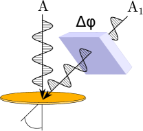
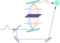
a) b) c)

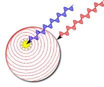
Figure 1: Suggested experimental geometries for control of optical channels. a) Geometry of monochromatic incident light fields approaching a disc shaped nanostructure to change the amplitudes of a specified principal mode, independent light sources with amplitudes $A$ and $A_{1}$ and a specified relative phase $\Delta\Phi$ are shown. b) A more general spatial-light modulator approach for changing phase and/or amplitude over a range of wavelengths for a broad-band source or applied pulse of light. c) Generation of phase controlled light from an internal source (driven in the blue) through a coherent process such as two photon decay or parametric down conversion, with external control light incident at the emission wavelength (in red). By exchanging red and blue, the same scheme can be used for second harmonic generation.

We can generalize Mie theory to non-spherical metallic and dielectric particles, provided that the particle does not posses sharp edges, and expand the electromagnetic field at any point in space (both inside and outside the structure) in terms of the intrinsic modes of the particle. These modes are in general combinations of different electric and magnetic multipoles Papoff and Hourahine (2011). As with the Mie modes of a sphere, the most important property here is that the projection on the surface of the particle of each scattering mode is spatially correlated to the projection of only one internal mode, and vice versa, where the spatial correlation is defined by an integral over the particle surface for the scalar product of the two projections (see Supplemental Material). Because of this property, the induced amplitudes of the $n^{\mathrm{th}}$ pair of principal modes of a nanostructure can be determined without need of noisy numerical inversion, by using the coupling of the surface projections of an incident field ($f$) to the internal ($i_{n}$) and scattered ($s_{n}$) mode pair as

$$a^{i}_{n}=\frac{i^{\prime}_{n}\cdot f}{i^{\prime}_{n}\cdot i_{n}},\;a^{s}_{n}=-\frac{s^{\prime}_{n}\cdot f}{s^{\prime}_{n}\cdot s_{n}},$$ (1)

here, $g\cdot h$ indicates the surface integral of the scalar product of the projected fields, $g$ and $h$. The sub-spaces of the internal and scattered modes are both orthonormal, i.e., $i_{n}\cdot i_{m}=s_{n}\cdot s_{m}=\delta_{nm}$ (with $\delta$ being the Kronecker delta), there are also associated dual modes:

$$i^{\prime}_{n}=\frac{i_{n}-(i_{n}\cdot s_{n})s_{n}}{\sqrt{1-(i_{n}\cdot s_{n})^{2}}},\;s^{\prime}_{n}=\frac{s_{n}-(i_{n}\cdot s_{n})i_{n}}{\sqrt{1-(i_{n}\cdot s_{n})^{2}}}$$ (2)

where $i^{\prime}_{n}\cdot i^{\prime}_{m}=s^{\prime}_{n}\cdot s^{\prime}_{m}=\delta_{nm}$, $i^{\prime}_{n}\cdot s_{n}=s^{\prime}_{n}\cdot i_{n}=0$ and $i^{\prime}_{n}\cdot i_{n}=s^{\prime}_{n}\cdot s_{n}$. Note that in this work that $i^{\prime}_{n}$ and $s^{\prime}_{n}$ are chosen to be unit vectors, as distinct from Ref. Papoff and Hourahine (2011). The spatial correlations between modes that appear in this theory can be interpreted geometrically, by introducing the principal cosines and sines, $i_{n}\cdot s_{n}=\cos{(\xi_{n})}$ and $i^{\prime}_{n}\cdot i_{n}=s^{\prime}_{n}\cdot s_{n}=\sin{(\xi_{n})}$. The relative orientation of the $n^{\mathrm{th}}$ set of modes are shown schematically in Figure 2. Correlations, princple vectors and coefficients $\{a^{i,s}\}$ depend on the wavelength parametrically through the frequency dependance of the dielectric and magnetic permittivity and permeability Papoff and Hourahine (2011).

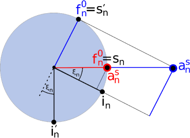
Figure 2: Induced amplitudes, $a_{n}^{s}$, of the $n^{\mathrm{th}}$ principal modes of a nanostructure, due to fields with projections parallel to $s_{n}$ (shown in red, corresponding to Eqn. 3) and $s^{\prime}_{n}$ (blue, matching Eqn. 4), all modes and incident fields have unit magnitide (marked circle).

From Eq. (1), one can see Papoff and Hourahine (2011) that strongly correlated, i.e., closely aligned modes are at the origin of resonances in nanoparticles as well as large transient gain and excess noise Firth and Yao (2005) in unstable optical cavities and classical or quantum systems governed by non-hermitian operators Papoff et al. (2008); Papoff and Robb (2012).

General geometrical considerations Farrell and Ioannou (1996) allow us to determine the surface fields which excite $s_{n}$ but not $i_{n}$ (or $i_{n}$ and not $s_{n}$), or that produce the largest amplitude for modes $s_{n}$ or $i_{n}$. We recall that any incident field can be decomposed as $f=f_{n}+f_{n_{\perp}}$, with $f_{n}$ the part of the incident field that couples only with the $n^{\mathrm{th}}$ modes and $f_{n_{\perp}}$ being the part that does not. We find that

$$f_{n}=s_{n}\rightarrow a^{s}_{n}=1,\;a^{i}_{n}=0,$$ (3)

$$f_{n}=s^{\prime}_{n}\rightarrow a^{s}_{n}=\frac{1}{\sin{(\xi_{n}})},\;a^{i}_{n}=-\frac{\cos{(\xi_{n})}}{\sin{(\xi_{n}})}.$$ (4)

Eqn. (3) give the requirement for incident fields that, irrespectively of $f_{n_{\perp}}$, produce excitation of only the scattering mode, i.e., null amplitude for the corresponding internal mode. Alternatively the largest amplitude of the scattering mode is obtained for fields with the form of Eq. (4). Note that we are considering only incident fields with $f_{n}\cdot f_{n}=1$ in Eqs. (3,4) to avoid trivial effects due to the overall amplitude of the incident fields. Figure 2 depicts the corresponding incident fields and the associated amplitudes of the scattered light in mode $s_{n}$ for both types of incident field. The analogous conditions for $i_{n}$ are found by exchanging $s$ with $i$ in Eqs. (3, 4).

Two points are worth noting. First, these are exact conditions for the surface fields that are valid at any frequency and have two possible applications: control of a mode (or modes) over a range of frequency and introduction of narrow band features in the spectral response of the particle. Second, the largest amplitude for a mode is not achieved through single mode excitation, but by an optimal excitation that produces amplitudes in the two principal modes of the channel. For physical applications it is necessary to generate incident fields which have tangent components that fulfill Eqs.(3), or (4). The case $f=s_{n}$ can be in principle realized through time reversal of the lasing mode of an amplifier with the same shape as the particle and gain opposite to the loss Noh et al. (2012) at the resonant frequency of the mode. To experimentally realize this is quite challenging, as radiation would need to converge towards the particle from all directions. We are instead interested in deriving general conditions for optimal excitation of modes at any frequency with easily accessible sources of radiation. In general, an incident field $F(\mathbf{r})$ with tangent components $f=i_{n}$ or $f=s_{n}$ cannot be realized using common sources of radiation external to the particle, such as laser beams or SNOM tips, or even internal sources such as fluorescent or active hosts. This is because these sources emit waves that are neither outgoing radiating waves in the external medium, as is the scattering mode, $s_{n}$, nor standing waves in the internal medium, such as the internal mode, $i_{n}$. However, by combining two or more of these sources with appropriate phases and amplitudes, it is possible to control in a simple and effective way the few dominant interaction channels of any nanoparticle. To construct fields to realise the conditions of Eqs. (3) or (4) requires two linearly independent incident fields, $Af$, and $A_{1}f^{1}$, both coupled to the channel $n$, such that

$$\frac{s_{n}\cdot f}{s_{n}\cdot f^{1}}\neq\frac{i_{n}\cdot f}{i_{n}\cdot f^{1}}.$$ (5)

The conditions for the suppression of $i_{n}$ or maximal excitation of $s_{n}$ are realized, up to a scale factor, by choosing $A_{1}$ as follows:

$$A_{1}=-A\frac{i_{n}\cdot f}{i_{n}\cdot f^{1}},$$ (6)

$$A_{1}=-A\frac{i^{\prime}_{n}\cdot f}{i^{\prime}_{n}\cdot f^{1}},$$ (7)

with $A$, $A_{1}$ being complex amplitudes that can be experimentally adjusted through phase plates and dicroic elements (Figure 1 suggests a geometry for constructing these fields, while Figure 4b) shows a numerical example of scanning the relative complex amplitude to produce specific scattered light). Analogous conditions for optimization of $i_{n}$ and suppression of $s_{n}$ can be found by swapping $i_{n},i^{\prime}_{n}$ with $s_{n},s^{\prime}_{n}$ in Eqs. (6, 7): the generalization of Eq. (6) to a larger number of modes is presented in the Supplemental Material.

We note that conservation of energy applies to the incident scattered and internal fields, but not necessarily to each interaction channel separately. However, if incident fields with $f_{n}\neq 0,f_{n_{\perp}}=0$ exist, the conservation of energy applies to the $n$ channel. From the Stratton-Chu representations Stratton and Chu (1939) (see Supplemental Information) we can show that in particles where the dependence of the electric (and magnetic) parts of $i_{n},s_{n},f_{n}$ on the surface coordinates is the same, such as for sphere and cylinders, the ratios in Eq. (5) depends on the flux of energy of the incident field into the particle, and Eq. (5) is always violated when the sources are both either outside or inside the particle. For instance, explicitly in the case of a sphere any external source can be expanded by the set of regular multipoles with angular indexes $l,m$, while any internal source is expanded by the set of radiating spherical multipoles, as shown in the Supplementary Material. In this case the amplitudes of internal and scattering modes cannot be controlled by independent external – or internal – sources: Eqs. (6,7) become equivalent and lead to the simultaneous suppression of both $i_{n}$ and $s_{n}$, while the maximization of the amplitudes of both scattering and internal modes is provided by ensuring that the contributions of the incident fields to the amplitudes add in phase. However, maximal excitation, Eq. (6), or suppression of a mode can be obtained also in these particles at any frequency provided one source is external and the other internal, or that one incident field is a regular wave with with a power flow of $W_{n}=0$ and the other an incoming wave with $W_{n}\neq 0$. Examples of internal sources important for applications are an impurity scattering inelastically at the same frequency as the external control beam or an active center excited non radiatively. Incoming waves are more difficult to realize, but could be in principle be obtained through time reversal techniques Pierrat et al. (2013).

We now show numerically how the theory developed here can be applied. In Figure 3 we show how we can suppress either the scattered or the internal mode of the resonant channel in a rounded rod-shaped particle, introducing in this way features that are much narrower than the resonance. The height and the position of this curves, the ”mode landscape” Papoff and Hourahine (2011) are a property of the particle, but the amplitude of the modes, which is color coded in the figure, depends also on the incident fields. The width of the narrow structure depends on the spectral resolution of the elements used in the set-up shown in Figure 1 b. This application leads to a much higher spectral resolution in surface enhanced spectroscopy and sensing. In Figure 4 we show how the angular momentum of the scattered light can be controlled in a gold disc. The disc has an electric dipole radiation pattern and by suppressing the channels with $m=\pm 1$, where $m$ is the eigenvalue of the angular momentum around the axis of the disc, we can make the disc virtually invisible in the far field. Using the same technique over a range of wavelengths we can control and manage the dipole resonance of this disc, introducing lines that have a full width half maximum one order of magnitude smaller than the width of the dipole resonance, see Figure 5.

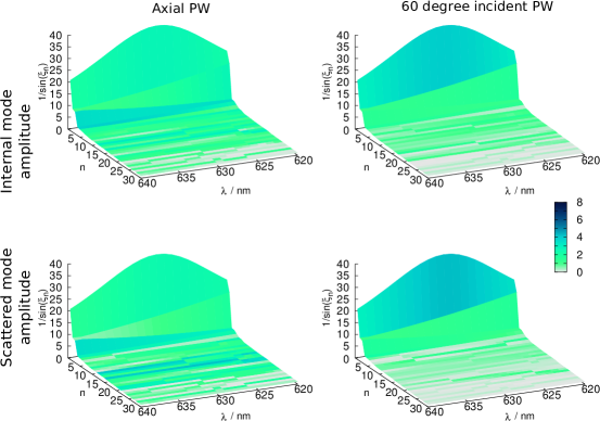
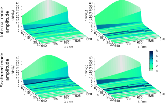
Figure 3: Internal and scattered mode amplitudes of a rounded rod-shaped dielectric ($n=1.5$) particle, of 2 $\mu$m length and 0.7 $\mu$m diameter around one of its (many) resonances at $\sim 630$ $nm$. The height of this landscape is $\sin^{-1}({\xi})$, i.e. the largest value of amplitude possible for $|f_{n}|=1$; while the shading of the traces overlaid on top show, for each wavelength ($\lambda$), the amplitude induced by the incident combinations for the first $n$ most aligned principle modes. For fields which obey Eqn. (5), the internal and scattered modes can be independently addressed. Here we use a second field with $60^{\circ}$ direction of incidence and polarisation, chosen to either cancel the peak of the resonant feature at the back of the landscape for the internal or scatted cases respectivly (leading to the disapearance of amplitude in only that particular mode).

a)

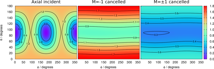
b)

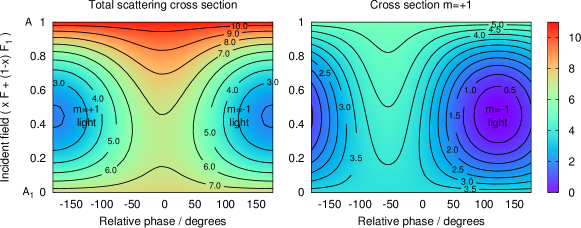
Figure 4: Differential scattering for a rounded disc shaped (20 nm thickness and 60 nm radius) gold disc, with a dominant single pair mode modes showing a dipolar resonance at 697 nm (in a surrounding medium Malitson (1965) with $\epsilon_{r}$ scaled by 0.75 to emulate support on a silica surface in air.) a) Scattering from an incident plane wave clearly shows a dipole radiation pattern, but this consists light with both $m=\pm 1$ angular momentum, by introducing a second and then third field with chosen complex amplitudes, the light in the $m=-1$ and then both $m\pm 1$ channels can be removed. b) Illustration of the effect of scanning for the condition to remove the $m=-1$ channel by adjusting the magnitude and phase of a second incident planewave. Experimentally, this example requires monitoring the orbital angular momentum of light emitted along the particle axis, to determine the relative amplitudes and phase where only the $m=-1$ dipolar resonance is active. Here we show the effect of scanning the relative amplitude and phase of axial and an additional $45^{\circ}$ direction (with respect to the particle axis) plane-polarised light, between being purely the axial ($x=1$, field A) and inclined ($x=0$, field $A_{1}$) incident light.

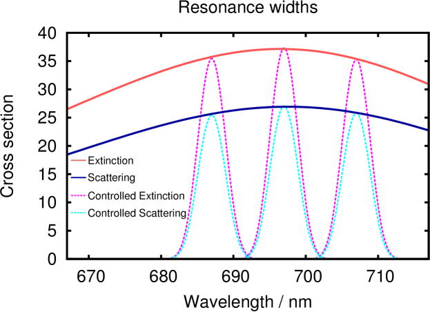
Figure 5: Cross sections of the gold disc from Figure 4 with standard axial incidence, leading to a broad feature in the extinction (red) and scattering (blue), this is compared again its response to illumination of light from three directions (axial, $45$ and $90^{\circ}$ incident) with their relative phases (but not amplitudes) modulated to cause constructive interference only at a chosen wavelength, then rotating the phase to cause destructive interference according to a gaussian envelope, producing a specified location and line width feature within the envelope of the original broad peak.

In conclusion we have shown that spatial distribution and angular momentum of internal and scattered fields of dielectric or metallic nanoparticles can be configured and optimized by controlling the amplitudes of a finite number of internal and scattered modes of the nanoparticle through the relative phases of coherent sources of light. This can be achieved using a single source of light of the type normally available in experiments, beam splitters and phase modulators, or combination of internal and external sources. The number of sources required is equal to the number of channels to control plus one, so this general approach is particularly simple to implement near resonances, where the response to light of nanoparticles is dominated by few modes. We have also been able to use optical control to reshape the spectral response of nanoparticles, introducing narrow spectral lines of a few nanometers width. In general, the width of the narrow lines depends on the spectral resolution of the control set-up, i.e. of the gratings and of the diffractive elements used and can be much narrower than the resonance peaks of the nanoparticle. This can significantly improve the spectral resolution of surface enhanced spectroscopy, which is based on the enhancement of surface fields near nanoparticles. The same control approach can be applied to light generated through linear and nonlinear processes by impurities embedded in the particle. In this case, controlling internal modes allows one the management of non-linear transitions in the impurities. Most of all, the potential of this work lies in its generality and in the fact that it does not requires complex spatial shaping of the incident fields, but only the control of their relative phases and amplitudes that can be provided by already available diffractive elements such as spatial light modulators.

Supplemental Information

We consider metallic and dielectric particles without sharp edges and use Holms et al. (2009) vectors, $F=[E,H]^{T}$, with three electric and three magnetic components for the electromagnetic fields; the corresponding surface field, $f$, is made up by the two electric and two magnetic components of $F$ tangent to the surface of the particle. In this notation, the boundary conditions are $f=f^{i}-f^{s}$, i.e. the tangent components $f$ of the incident field are equal to the difference between the tangent components of internal and scattered fields, $f^{i}$ and $f^{s}$ at the surface. We can find solutions of the Maxwell ’s equation in the internal and external media, the principal modes ${I_{n}},{S_{n}}$, such that the expansion of the scattered and internal fields converge to the exact fields for any incident field Rother et al. (2002); Holms et al. (2009); Papoff and Hourahine (2011). The tangent components of the principal modes, $\{i_{n}\}$ and $\{s_{n}\}$, form bases for the internal and scattered surface fields that are orthonormal with respect to the scalar product $f\cdot g=\sum_{j=1}^{4}\int_{S}f_{j}^{*}g_{j}ds$, where $j$ labels the components of the surface fields and the asterisk stands for the complex conjugate. Each pair $i_{n},s_{n}$ define an interaction channel for the particle that is independent from all the other pairs because each internal mode $i_{n}$ is orthogonal to all but the scattering mode $s_{n}$ and viceversa. The spatial correlations that appear in this theory can be interpreted geometrically. The principal cosine between $s_{n}$ and $i_{n}$ is defined by the overlap integral, or correlation Hannan (1961/1962), as $\cos{(\xi_{n})}\equiv i_{n}\cdot s_{n}$, with the arbitrary phases of $i_{n},s_{n}$ chosen so that the integral is either positive or null. The corresponding function $\sin{(\xi_{n})}$ is the orthogonal distance between $s_{n}$ and $i_{n}$. The angles ${\xi_{n}}$ characterize the geometry of the subspaces of the internal and scattered solutions and are invariant under unitary transformations Knyazev et al. (2010).

Given the importance of spheres in scattering, we show explicitly how the optimization or suppression of either scattering or internal modes can be obtained when one source is internal and the other external, but when not both sources are either internal or external. The internal and scattering modes used in this work are proportional to the usual Mie modes: writing explicitly the electric and magnetic component, the magnetic multipole modes are defined, up to an arbitrary phase factor, as

$$i_{lm}=\frac{e^{i\phi_{l}}}{(|i^{E}_{l}(r)|^{2}+|i^{H}_{l}(r)|^{2})^{1/2}}[m_{lm}(\Omega)i^{E}_{l}(r),n_{lm}(\Omega)i^{H}_{l}(r)]^{T},$$

$$s_{lm}=\frac{1}{(|s^{E}_{l}(r)|^{2}+|s^{H}_{l}(r)|^{2})^{1/2}}[m_{lm}(\Omega)s^{E}_{l}(r),n_{lm}(\Omega)s^{H}_{l}(r)]^{T}$$ (8)

where $r$ is the radius of the sphere, $\Omega$ the solid angle, $k_{i},k$ are the wavenumbers for internal and external medium, respectively, $m_{lm},n_{lm}$ vector spherical harmonics. $i^{E}_{l}(r)=j_{l}(k_{i}r)$, $i^{H}_{l}(r)=-i(\epsilon_{i}/\mu_{i})^{1/2}(k_{i}r)^{-1}\partial_{k_{i}r}k_{i}rj_{l}(k_{i}r)$, $s^{E}_{l}(r)=h_{l}(kr)$, $s^{H}_{l}(r)=-i(\epsilon/\mu)^{1/2}(kr)^{-1}\partial_{kr}krh_{l}(kr)$, $j_{l},h_{l}$ the spherical Bessel and Hankel functions of order $l$. $\phi_{l}=-Im\{\log{[{i^{E}_{l}(r)}^{*}s^{E}_{l}(r)+{i^{H}_{l}(r)}^{*}s^{H}_{l}(r)]}\}$ is such that

$$i_{lm}\cdot s_{lm}=\frac{{|i^{E}_{l}(r)}^{*}s^{E}_{l}(r)+{i^{H}_{l}(r)}^{*}s^{H}_{l}(r)|}{(|i^{E}_{l}(r)|^{2}+|i^{H}_{l}(r)|^{2})^{1/2}(|s^{E}_{l}(r)|^{2}+|s^{H}_{l}(r)|^{2})^{1/2}}.$$ (9)

Electric multipole modes are obtained as usual exchanging magnetic with electric parts. The incident fields generated by two external sources can be expanded in terms of electric and magnetic multipoles centered on the sphere; the only terms of these expansions that can couple to the modes in Eqs. (8) are $f=a[m_{lm}(\Omega)f_{l}^{E}(kr),n_{lm}(\Omega)f_{l}^{H}(kr)]^{T}$, $f^{1}=a_{1}[m_{lm}(\Omega)f_{l}^{E}(kr),n_{lm}(\Omega)f_{l}^{H}(kr)]^{T}$, where $f_{l}^{E}(kr),f_{l}^{H}(kr)$ are found by replacing $k_{i}r$ with $kr$ in $i^{E}_{l},i^{H}_{l}$ . Therefore we find that both terms in Eq. (5) are equal to $a/a_{1}$, i.e. the inequality is violated. On the contrary, the equality can be satisfied when the two sources are such that ${f_{l}^{1}}^{E}\neq f_{l}^{E},{f_{l}^{1}}^{H}\neq{f_{l}}^{H}$. This is the case when one source is external and the other is a radiating multipole inside the particle with $f^{1}=a_{1}[m_{lm}(\Omega){f_{l}^{1}}^{E}(k_{i}r),n_{lm}(\Omega){f_{l}^{1}}^{H}(k_{i}r)]^{T}$, where ${f_{l}^{1}}^{E}(k_{i}r),{f_{l}^{1}}^{H}(k_{i}r)$ are found by replacing $kr$ with $k_{i}r$ in $s^{E}_{l},s^{H}_{l}$. For this combination of internal and external sources Eqs. (6, 7), for suppression of $i_{lm}$ and maximal excitation of $s_{lm}$, can be applied and are

$$A_{1} = -A\frac{{f_{l}^{E}}^{*}i_{l}^{E}+{f_{l}^{H}}^{*}i_{l}^{H}}{{f_{l}^{1}}^{E*}i_{l}^{E}+{f_{l}^{1}}^{H*}i_{l}^{H}},$$ (10)

$$A_{1} = -A\frac{{f_{l}^{E}}^{*}(e^{i\phi_{l}}i_{l}^{E}-\cos{(\xi_{n})}s_{l}^{E})+{f_{l}^{H}}^{*}(e^{i\phi_{l}}i_{l}^{H}-\cos{(\xi_{n})}s_{l}^{E})}{{f_{l}^{1}}^{E*}(e^{i\phi_{l}}i_{l}^{E}-\cos{(\xi_{n})}s_{l}^{E})+{f_{l}^{1}}^{H*}(e^{i\phi_{l}}i_{l}^{H}-\cos{(\xi_{n})}s_{l}^{E})}.$$ (11)

The same analysis holds true also for infinite cylinders.

We consider here when an field generated by external source with $f_{n},\neq 0,f_{n_{\perp}}=0$ exist. Because $i_{n},s_{n},f_{n}$ are exact solutions of the Maxwell’s equations, the Stratton-Chu representation Stratton and Chu (1939) for particles with continuously varying tangents (particles of class $C^{1}$), and the corresponding jump relations Doicu et al. (2000) at the boundary of the particle

$$\int\nabla\times(n(y)\times i_{n}(y))g(x,y,k_{i})da(y)=\frac{1}{2}n(x)\times(n(x)\times i_{n}(x))$$ (12)

$$\int\nabla\times(n(y)\times s_{n}(y))g(x,y,k)da(y)=-\frac{1}{2}n(x)\times(n(x)\times s_{n}(x))$$ (13)

$$\int\nabla\times(n(y)\times f_{n}(y))g(x,y,k)da(y)=\frac{1}{2}n(x)\times(n(x)\times f_{n}(x)),$$ (14)

with $x,y$ points on the surface and $n(x)$ the outgoing normal at $x$. Using the Eqs.(12),(13) in Eq.(14) and the conservation of energy, we find

$$\int\nabla\times(n(y)\times i_{n}(y))g(x,y,k)da(y)=\frac{1}{2}n(x)\times(n(x)\times i_{n}(x))$$

$$-\frac{a^{s}_{n}}{a^{i}_{n}}n(x)\times(n(x)\times s_{n}(x))$$ (15)

$$W_{n}=|a^{i}_{n}|^{2}W^{i}_{n}+|a^{s}_{n}|^{2}W^{s}_{n}+$$

$$\frac{1}{2}Re[|a^{i}_{n}||a^{s}_{n}|e^{i\Delta}\int n(y)\cdot(i_{n}^{E}(y)\times s_{n}^{H*}(y))da(y)+$$

$$|a^{i}_{n}||a^{s}_{n}|e^{i\Delta}\int n(y)\cdot(s_{n}^{E}(y)\times i_{n}^{H*}(y))]da(y)=0,$$ (16)

where $\Delta$ is the phase difference between $a^{i}_{n},a^{s}_{n}$ and $W_{n},W^{i}_{n},W^{s}_{n}$ the power fluxes of $f_{n},i_{n},s_{n}$. Because $|a^{i}_{n}|,|a^{s}_{n}|$ and $\Delta$ do not depend on $x$, we can see that Eqs.(15),(16) can be solved only if the dependence on $x$ in all the terms in (15) can be factored out. This happens for spheres and cylinders.

The procedure in Eq. (6) is generalized to $m$ internal modes and $l$ scattering modes using $m+l$ incident fields, $A_{1}f^{1},\dots,A_{m+l}f^{m+l}$, each satisying Eq. (5), as follows

$$\left[\begin{array}[]{ccc}\frac{i^{\prime}_{1}\cdot f^{1}}{\sin{(\xi_{1})}}&\dots&\frac{i^{\prime}_{1}\cdot f^{m+l}}{\sin{(\xi_{1})}}\\ \vdots&&\vdots\\ \frac{s^{\prime}_{l}\cdot f^{1}}{\sin{(\xi_{l})}}&\dots&\frac{s^{\prime}_{l}\cdot f^{m+n}}{\sin{(\xi_{l})}}\end{array}\right]\left[\begin{array}[]{c}A_{1}\\ \vdots\\ A_{m+l}\end{array}\right]=-A\left[\begin{array}[]{c}\frac{i^{\prime}_{1}\cdot f}{\sin{(\xi_{1})}}\\ \vdots\\ \frac{s^{\prime}_{l}\cdot f}{\sin{(\xi_{l})}}\end{array}\right].$$ (26)

The solution for the amplitudes is unique if the determinant of the matrix is not null.

References

- Abb et al. (2011) Abb, M.; Albella, P.; Aizpurua, J.; Muskens, O. Nano Lett. 2011, 11,, 2457–2463.
- Kubo et al. (2005) Kubo, A.; Onda, K.; Petek, H.; Sun, Z.; Jung, Y.; Kim, H. Nano Lett. 2005, 5, 1123–1127.
- Durach et al. (2007) Durach, M.; Rusina, A.; Stockman, M. Nano Lett. 2007, 7, 3145–3149.
- Martin Aeschlimann et al. (2007) Martin Aeschlimann, M.; Bauer, M.; Bayer, D.; Tobias Brixner, T.; Garcı´a de Abajo, F.; Pfeiffer, W.; Rohmer, M.; Spindler, C.; Felix Steeb, F. Nature 2007, 446, 301–304.
- Noh et al. (2012) Noh, H.; Chomg, Y.; Stone, A.; Cao, H. Phys. Rev. Lett. 2012, 108, 186805.
- Pierrat et al. (2013) Pierrat, R.; Vandenbem, C.; Fink, M.; Carminati, R. Phys. Rev. A 2013, 87, 041801.
- Jeffers (2000) Jeffers, J. Journ. Mod. Opt. 2000, 47, 1819–1824.
- Zhang et al. (2012) Zhang, J.; MacDonald, K.; Zheludev, N. Light: Science & Appl. 2012, 1, e18.
- Papoff and Hourahine (2011) Papoff, F.; Hourahine, B. Opt.Express 2011, 19, 21432–21444.
- Doherty et al. (2013) Doherty, M.; Murphy, A.; Pollard, R.; Dawson, P. Phys. Rev. X 2013, 3, 011001.
- Firth and Yao (2005) Firth, W. J.; Yao, A. Phys. Rev. Lett. 2005, 95, 073903.
- Papoff et al. (2008) Papoff, F.; D’Alessandro, G.; Oppo, G.-L. Phys. Rev. Lett. 2008, 100, 123905.
- Papoff and Robb (2012) Papoff, F.; Robb, G. Phys. Rev. Lett. 2012, 108, 113902.
- Farrell and Ioannou (1996) Farrell, B. F.; Ioannou, P. J. Journ. of Atm. Sc. 1996, 53, 2025–2040.
- Stratton and Chu (1939) Stratton, J. A.; Chu, L. J. Phys. Rev. 1939, 56, 99–107.
- Malitson (1965) Malitson, I. Journal of the Optical Society of America 1965, 55, 1205–1209.
- Holms et al. (2009) Holms, K.; Hourahine, B.; Papoff, F. J. Opt. A: Pure Appl. Opt. 2009, 11, 054009.
- Rother et al. (2002) Rother, T.; Kahnert, M.; Doicu, A.; Wauer, J. Prog. Electromag. Res. 2002, 38, 47–95.
- Hannan (1961/1962) Hannan, E. J. Aust. Math. Soc. 1961/1962, 2, 229–242.
- Knyazev et al. (2010) Knyazev, A.; Jujusnashvili, A.; Argentati, M. Journ. of Func. Analys. 2010, 259, 1323–1345.
- Doicu et al. (2000) Doicu, A.; Eremin, Y.; Wreidt, T. Acoustic and Electromagnetic Scattering Analysis Using Discrete Sources; Accademic Press, 2000.