Temperature Modulation of the Transmission Barrier in Quantum Point Contacts

Abstract

We investigate near-equilibrium ballistic transport through a quantum point contact (QPC) along a GaAs/AlGaAs heterojunction with a transfer matrix technique, as a function of temperature and the shape of the potential barrier in the QPC. Our analysis is based on a three-dimensional (3D) quantum-mechanical variational model within the Hartree-Fock approximation that takes into account the vertical depletion potential from ionized acceptors in GaAs and the gate-induced transverse confinement potential that reduce to an effective slowly-varying one-dimensional (1D) potential along the narrow constriction. The calculated zero-temperature transmission exhibits a shoulder ranging from 0.3 to 0.6 depending on the length of the QPC and the profile of the barrier potential. The effect is a consequence of the compressibility peak in the 1D electron gas and is enhanced for anti-ferromagnetic interaction among electrons in the QPC, but is smeared out once temperature is increased by a few tenths of a kelvin.

I Introduction

A quantum point contact (QPC) is a narrow constriction in a two-dimensional electron gas (2DEG). QPCs are commonly realized in GaAs/AlGaAs heterostructures by applying a negative voltage to a split metallic gate placed on top of the device. This leads to the depletion of the electron gas directly underneath the gate, leaving only a narrow channel between two 2DEG reservoirs (acting as source and drain), with a width that can be modulated by the gate bias (see Figure 1, top left). Experiments have shown that the QPC conductance is quantized in units ofWharam et al., 1988; van Wees et al., 1988; Thomas et al., 1996 $G_{0}\equiv 2e^{2}/h$. This phenomenon is a direct consequence of quantum-mechanical 1D transmission through a saddle potential, for which the product of the carrier velocity and 1D density of states is energy independent. As a result, discrete steps appear whenever a new 1D channel (1D energy subband) becomes populated for conductionGlazman et al., 1988; Büttiker, 1990. In addition to the quantized conductance, an anomalous conductance plateau has been observed around $0.7G_{0}$Thomas et al., 1996; Nuttinck et al., 2000. Of particular interest is the fact that this plateau, dubbed the 0.7 structure or anomaly, becomes stronger as temperature increases above $0\,\mathrm{K}$, reaching its maximum strength at $T\sim 1-2\,\mathrm{K}$ and vanishing by $T\sim 10\,\mathrm{K}$ due to thermal smearingThomas et al., 1996, 1998.

There is substantial agreement that the 0.7 structure is a consequence of many-body effects, but the precise cause of this phenomenon is still the subject of significant debateBerggren and Pepper, 2010; Micolich, 2011. One possible explanation involves a Kondo-like effect due to the formation of a quasi-bound state in the QPCCronenwett et al., 2002; Meir et al., 2002. Alternatively, it has been proposed that a static spin polarization is present along the constrictionThomas et al., 1996, 1998; Rokhinson et al., 2006. However, theoretical calculations based on spin density-functional theory (DFT) have been inconclusive. While several works favor the formation of a bound stateMeir et al., 2002; Hirose et al., 2003; Rejec and Meir, 2006; Ihnatsenka and Zozoulenko, 2007; Meir, 2008, others argue against itStarikov et al., 2003; Berggren and Yakimenko, 2008 and support the presence of a static spin polarizationStarikov et al., 2003; Havu et al., 2004; Berggren and Yakimenko, 2008. To add to the controversy, it has been suggested that Kondo correlations may coexist with static spin polarization due to the presence of localized, ferromagnetically-coupled magnetic impurity states at the QPCSong and Ahn, 2011.

In this work, we re-examine the electron transmission through a QPC along a GaAs/AlGaAs heterojunction by using a three-dimensional (3D) self-consistent model that takes into account the lateral confinement and the potential barrier induced by the gates as well as the band bending near the GaAs/AlGaAs interface. The system is not treated as strictly two-dimensional, which allows us to consider the variation of the vertical confinement on the 2D constriction and the resulting changes in the conductance. A key issue in our approach is the assumption that the confinement along the 1D channel is slowly-varying (adiabatic). For this reason, we first solve the 3D many-body effects of a 1D channel in the Hartree-Fock approximation to show that tunneling of electrons through the QPC can be reduced to an effective 1D potential. In our model, variational wavefunction parameters and the effective potential are obtained self-consistently as a function of the gate voltage, confinement strength and temperature. We then use the transfer matrix techniqueJonsson and Eng, 1990 to obtain the transmission coefficient and the conductance through the QPC barrier. We show that, at $T=0$, the conductance through the QPC exhibits a kink or feature occurring between $0.3$ and $0.6G_{0}$, depending on the profile of the potential barrier. The kink is caused by a pinning of the effective potential when the electron gas in the region of the QPC is depleted, and disappears as temperature increases.

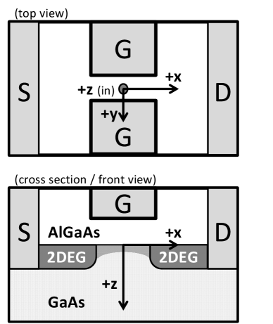
Figure 1: Schematic representation of a quantum point contact. S, D and G stand for source, drain and gate, respectively.

II QPC Structure Model

A quantum point contact is usually achieved along a GaAs/AlGaAs heterojunction, which consists of a layer of modulation-doped or delta-doped AlGaAs on top of a GaAs substrate. The heterojunction interface is about 200-300 nm below the surfaceThomas et al., 1995; Cronenwett, 2001. A cross-section of the structure is shown in Figure 1 with the $z$-axis perpendicular to the hetero-interface, oriented so that $z>0$ measures the depth in the GaAs substrate. Because of the doping, charge carriers are confined into a 2DEG underneath the GaAs/AlGaAs heterojunction interface (in the $x-y$ plane) by the depletion potential $U_{A}$ resulting from the GaAs ionized acceptors. Meanwhile, the tall hetero-barrier prevents electrons from tunneling into AlGaAs ($z<0$)Ando et al., 1982. Lateral confinement is achieved along the $y$-direction by applying a negative potential on the split-gate electrodes (Fig. 1). Electron energies are restricted to discrete subbands which, at zero temperature, will be occupied only if their energies are below the Fermi energy.

A top view of the transport configuration is shown schematically in Figure 1. The $x$-direction runs between the source and drain electrodes, while the $y$-axis extends from one gate to the other. The center of the QPC is at $\left(x,y\right)=\left(0,0\right)$. Electrons are injected into the QPC from the 2DEG on the source side of the structure and collected at the drain. As a consequence of the finite width of the negatively-biased gate electrodes, there is a saddle potential $U_{\mathrm{QPC}}\left(x,y\right)$ in the QPC that results from two contributions: first, the potential energy well $U_{\mathrm{well}}$, which we model as parabolic (see Fig. 2(a)), confines electrons to a narrow channel between the gates along the $y$-direction, and splits each of the 2DEG subbands (with energies $E_{z0}$, $E_{z1}$,… away from the QPC for $x\rightarrow-\infty$) into a new set of discrete 1D energy subbands with energies $E_{y0}$, $E_{y1}$,… above those of the 2DEG subbands. Second, there is also a smooth potential barrier $U_{x}$ running along the $x$-direction. Due to the saddle potential, the charge density at the QPC decreases, which in turn reduces the effect of electron-electron interactions and shifts the 2DEG subband energies downwards. The addition of the energy $E_{z0}$ of the lowest 2DEG subband (Fig. 2(b)), the (smallest) energy increase $E_{y0}$ from the parabolic confinement, and the QPC potential barrier $U_{x}$, results in an effective 1D potential $U_{\mathrm{eff}}$, as shown in Fig. 2(c).

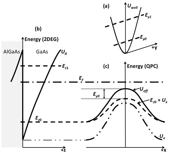
Figure 2: (a) Confinement potential well $U_{\mathrm{well}}$ induced by the gates, showing the energy sub-levels $E_{y0}$, $E_{y1}$, etc. (b) Potential in the 2DEG, showing the Fermi energy and the 2DEG subbands. (c) Contributions to the effective potential: energy of the lowest subband ($E_{z0}$), potential barrier ($U_{x}$) and energy due to the parabolic confinement ($E_{y0}$).

In our study we limit ourselves to the lowest-energy subband and include the Coulomb and exchange interactions ($U_{\mathrm{el}}$ and $U_{\mathrm{exch}}$, respectively) within the Hartree-Fock approximation. The Fermi energy $E_{F}$ is pinned at the source electrode, whereas the Fermi level at the drain is shifted from this value by a small applied source-drain bias. We neglect the spin-orbit (Rashba) interaction $\hat{H}_{so}=\alpha\left(\hat{\boldsymbol{\sigma}}\times\hat{\mathbf{p}}\right)_{z}/\hbar$ , as its contribution to the effective potential in GaAs will be much smaller than in other materials. The Rashba coupling constant in GaAs is $\alpha=\left(0.052\,\mathrm{e\cdot nm^{2}}\right)F_{z}$ (where $F_{z}$ is the electric field in the $z$-direction), which is significantly less than in InAs ($\left(1.17\,\mathrm{e\cdot nm^{2}}\right)F_{z}$) and in InSb ($\left(5.23\,\mathrm{e\cdot nm^{2}}\right)F_{z}$)Winkler, 2003. We also neglect the image potential, considering the relatively small difference between the dielectric constants of GaAs ($\kappa=12.9$) and $\mathrm{Al_{x}Ga_{1-x}As}$ ($\kappa=12.0$ for $x=0.3$).

III 3D Hartree-Fock Model of Modulation-Doped 1D GaAs Channels

Before solving for the electronic properties in the QPC we consider the case of a very long constriction, effectively a 1D channel or quantum wire. In this case, the system is translationally invariant along the $x$-direction and the QPC potential barrier $U_{x}$ in the wire is reduced to a constant value $U_{0}$.

In the absence of an applied split-gate voltage, the (2DEG) confinement potential in GaAs due to the depletion from ionized acceptors is well approximated byAndo et al., 1982 $U_{\mathrm{A}}\left(z\right)=\frac{q^{2}N_{A}}{\epsilon}z\left(z_{d}-\frac{z}{2}\right)$; here, $q$ is the electron charge, $\epsilon$ is the GaAs dielectric constant, $N_{A}$ is the acceptor density and $z_{d}=\sqrt{2\epsilon E_{C}/q^{2}N_{A}}$ is the width of the depletion region ($E_{C}$ being the bottom of the conduction band in the bulk of GaAs). This potential satisfies the boundary conditions $\left[\partial U_{A}/\partial z\right]\left(z=z_{d}\right)=0$ (i.e . the electric field is zero at $z=z_{d}$) and $U_{A}\left(z=0\right)=0$. The parabolic confining potential induced by the applied gate voltage is given by $U_{\mathrm{well}}\left(y\right)=m^{*}\omega_{y}^{2}y^{2}/2$, where $\omega_{y}$ represents the strength of the confinement.

With these confining potentials, the Schrödinger equation within the Hartree-Fock approximation reads

$$-\frac{\hbar^{2}}{2m^{*}}\nabla^{2}\psi_{\left\{i\right\}}\left(\vec{r}\right)+\left[U_{A}\left(z\right)+U_{\mathrm{well}}\left(y\right)+U_{x}+\right.\\ \left.U_{\mathrm{el}}\left(\vec{r}\right)\right]\psi_{\left\{i\right\}}\left(\vec{r}\right)+\hat{U}_{\mathrm{exch}}\left[\psi_{\left\{j\right\}}\left(\vec{r}\right)\right]=E_{\left\{i\right\}}\psi_{\left\{i\right\}}\left(\vec{r}\right)$$ (1)

where the quantum numbers $\left\{i\right\}=\left\{i_{x},i_{y},i_{z},\sigma_{i}\right\}$ ($\sigma$ being the electron spin) are associated with the eigenenergies $E_{\left\{i\right\}}$. The Hartree (direct) term $U_{\mathrm{el}}$ and the exchange term $\hat{U}_{\mathrm{exch}}$ read, respectively:

$$U_{\mathrm{el}}\left(\vec{r}\right)\psi_{\left\{i\right\}}\left(\vec{r}\right) = \hphantom{\textnormal{-}}\sum_{\left\{j\right\}}\int\mathrm{d}^{3}\vec{r}^{\,\prime}\left|\psi_{\left\{j\right\}}\left(\vec{r}^{\,\prime}\right)\right|^{2}U_{\mathrm{Coul}}\left(\vec{r},\vec{r}^{\,\prime}\right)\psi_{\left\{i\right\}}\left(\vec{r}\right)$$ (2)

$$\hat{U}_{\mathrm{exch}}\left[\psi_{\left\{j\right\}}\left(\vec{r}\right)\right] = \textnormal{-}\sum_{\left\{j\right\}}\int\mathrm{d}^{3}\vec{r}^{\,\prime}\,\psi_{\left\{j\right\}}^{*}\left(\vec{r}^{\,\prime}\right)U_{\mathrm{Coul}}\left(\vec{r},\vec{r}^{\,\prime}\right)\psi_{\left\{i\right\}}\left(\vec{r}^{\,\prime}\right)\psi_{\left\{j\right\}}\left(\vec{r}\right)\delta_{\sigma_{i}\sigma_{j}}$$ (3)

$U_{\mathrm{Coul}}$, the Coulomb interaction, is given by

$$U_{\mathrm{Coul}}\left(\vec{r},\vec{r}^{\,\prime}\right)=\frac{q^{2}}{4\pi\epsilon}\left(\frac{1}{\left|\vec{r}^{\,\prime}-\vec{r}\right|}-\frac{1}{\sqrt{\left(x^{\prime}-x\right)^{2}+\left(y^{\prime}-y\right)^{2}+\left(z^{\prime}+z\right)^{2}}}\right)$$ (4)

The second term on the right-hand side corresponds to mirror charges placed on the AlGaAs side of the interface. With this expression for $U_{\mathrm{Coul}}$, $U_{\mathrm{el}}\left(\vec{r}\right)$ satisfies boundary conditions similar to those of $U_{A}$, i.e. $U_{\mathrm{el}}\left(z=0\right)=0$ and $\left[\partial U_{\mathrm{el}}/\partial z\right]_{z=z_{d}}\approx\left[\partial U_{\mathrm{el}}/\partial z\right]_{z\rightarrow\infty}=0$. (This will also ensure that the expectation value $\left\langle U_{\mathrm{el}}\right\rangle$ remains finite.) The occupation number of a state with energy $E$ is given by the Fermi-Dirac distribution, $f_{T}\left(E\right)=\left\{1+\exp\left[\left(E-\mu\right)/k_{B}T\right]\right\}^{-1}$, where $\mu$ is the chemical potential (which equals $E_{F}$ at $T=0$).

Since $U_{x}\left(=U_{0}\right)$ is constant, the solution to Eq. (1) can be written as a product of a plane wave traveling along $x$ and a function depending on $y$ and $z$, i.e. $\psi_{\left\{k_{x},i_{y},i_{z},\sigma_{i}\right\}}=\left(\mathrm{e}^{\mathrm{i}k_{x}x}/\sqrt{L_{x}}\right)\Lambda_{i_{y},i_{z}}\left(y,z\right)$, where $L_{x}$ is the length of the wire. With this assumption, the $y$- and $z$-dependence in Eq. (1) can be separated, yielding

$$\left\{-\frac{\hbar^{2}}{2m^{*}}\left(\partial_{y}^{2}+\partial_{z}^{2}\right)U_{A}\left(z\right)+U_{\mathrm{well}}\left(y\right)+U_{x}+U_{\mathrm{el}}\left(y,z\right)\right\}\Lambda_{i_{y},i_{z}}\left(y,z\right)\\ +\hat{U}_{\mathrm{exch}}\left[\Lambda_{j_{y},j_{z}}\left(y,z;k_{x},\sigma_{j}\right)\right]=\left\{E\left(k_{x},i_{y},i_{z},\sigma_{i}\right)-\frac{\hbar^{2}k_{x}^{2}}{2m^{*}}\right\}\Lambda_{i_{y},i_{z}}\left(y,z\right)$$ (5)

where, after expanding $U_{\mathrm{Coul}}$ (Eq. (4)) in a Fourier series, the Hartree and exchange terms are respectively given by

$$U_{\mathrm{el}}\left(y,z\right)=\sum_{p_{x},j_{y},j_{z},\sigma_{j}}\int\mathrm{d}y^{\prime}\int\mathrm{d}z^{\prime}\left|\Lambda_{j_{y},j_{z}}\left(y^{\prime},z^{\prime}\right)\right|^{2}\frac{1}{L_{x}}\int\frac{\mathrm{d}p_{y}}{p_{y}}\mathrm{e}^{\mathrm{i}p_{y}\left(y^{\prime}-y\right)}\left[\mathrm{e}^{-p_{y}\left|z^{\prime}-z\right|}-\mathrm{e}^{-p_{y}\left(z^{\prime}+z\right)}\right]$$ (6)

$$\hat{U}_{\mathrm{exch}}\left[\Lambda_{j_{y},j_{z}}\left(y,z;k_{x},\sigma_{j}\right)\right] = \textnormal{-}\sum_{p_{x},j_{y},j_{z},\sigma_{j}}\delta_{\sigma_{i}\sigma_{j}}\int\mathrm{d}y^{\prime}\int\mathrm{d}z^{\prime}\,\Lambda_{j_{y},j_{z}}^{*}\left(y^{\prime},z^{\prime}\right)\Lambda_{i_{y},i_{z}}\left(y^{\prime},z^{\prime}\right)\Lambda_{j_{y},j_{z}}\left(y,z\right)$$ (7)

$$\cdot\frac{1}{L_{x}}\int\frac{\mathrm{d}p_{y}}{\bar{p}_{y}}\mathrm{e}^{\mathrm{i}p_{y}\left(y^{\prime}-y\right)}\left[\mathrm{e}^{-\bar{p}_{y}\left|z^{\prime}-z\right|}-\mathrm{e}^{-\bar{p}_{y}\left(z^{\prime}+z\right)}\right]$$

with $\bar{p}_{y}\equiv\sqrt{\left(p_{x}-k_{x}\right)^{2}+p_{y}^{2}}$. We take the expectation value of the left-hand side of Eq. (5) and we define two new potential energies: $E_{yz}$, which corresponds to the carrier kinetic energy and the confinement along the y- and z-directions, and $U_{\mathrm{ee}}$, which corresponds to electron-electron interactions:

$$E_{yz}\equiv\left\langle-\frac{\hbar^{2}}{2m^{*}}\left(\partial_{y}^{2}+\partial_{z}^{2}\right)\right\rangle+\left\langle U_{\mathrm{well}}\right\rangle+\left\langle U_{A}\right\rangle$$ (8)

$$U_{\mathrm{ee}}\equiv\left\langle U_{\mathrm{el}}\right\rangle+\left\langle\hat{U}_{\mathrm{exch}}\right\rangle$$ (9)

Then, we define the effective 1D potential as

$$U_{\mathrm{eff}}\left(k_{x},i_{y},i_{z},\sigma_{i}\right)=\\ U_{x}+E_{yz}\left(i_{y},i_{z}\right)+U_{\mathrm{ee}}\left(k_{x},i_{y},i_{z},\sigma_{i}\right)$$ (10)

so that the 1D electron energy reads

$$E\left(k_{x},i_{y},i_{z},\sigma_{i}\right)=\frac{\hbar^{2}k_{x}^{2}}{2m^{*}}+U_{\mathrm{eff}}\left(k_{x},i_{y},i_{z},\sigma_{i}\right)$$ (11)

To study the extreme quantum limit, when only the lowest-energy subband is occupied, we use the trial wave function defined as

$$\Lambda_{00}\left(y,z\right)=\left(\frac{a^{\nicefrac{{1}}{{2}}}}{\pi^{\nicefrac{{1}}{{4}}}}\mathrm{e}^{-a^{2}y^{2}/2}\right)\left(\frac{b^{\nicefrac{{3}}{{2}}}}{2^{\nicefrac{{1}}{{2}}}}z\mathrm{e}^{-bz/2}\right)$$ (12)

where the parameters $a$ and $b$ are determined by the variational method. The first term of the right-hand side is the ground state of the parabolic potential $U_{\mathrm{well}}$, while the second term approximates the ground state of the depletion potential $U_{A}$. Then, we obtain the following expectation values for the different terms in the effective potential $U_{\mathrm{eff}}$:

$$\left\langle-\frac{\hbar^{2}}{2m^{*}}\left(\partial_{y}^{2}+\partial_{z}^{2}\right)\right\rangle\equiv\left\langle\hat{T}_{yz}\right\rangle=\frac{\hbar^{2}}{8m^{*}}\left(2a^{2}+b^{2}\right)$$ (13a)

$$\left\langle U_{\mathrm{well}}\right\rangle+\left\langle U_{A}\right\rangle=\frac{m^{*}\omega_{y}^{2}}{4a^{2}}+\frac{3q^{2}N_{A}z_{d}}{\epsilon b}\left(1-\frac{2}{z_{d}b}\right)$$ (13b)

$$\left\langle U_{\mathrm{el}}\right\rangle=\frac{q^{2}}{16\pi^{2}\epsilon}\zeta_{ab}\left(0\right)\int_{-\infty}^{+\infty}\mathrm{d}p_{x}\,f_{T}\left[E\left(p_{x}\right)\right]=\frac{q^{2}\zeta_{ab}\left(0\right)}{16\pi\epsilon}n_{0}$$ (13c)

$$\left\langle\hat{U}_{\mathrm{exch}}\left(k_{x}\right)\right\rangle=-\frac{q^{2}}{32\pi^{2}\epsilon}\int_{-\infty}^{+\infty}\mathrm{d}p_{x}\,\zeta_{ab}\left(p_{x}-k_{x}\right)f_{T}\left[E\left(p_{x}\right)\right]$$ (13d)

Here, $n_{0}=\frac{1}{\pi}\int_{-\infty}^{+\infty}\mathrm{d}k\,f_{T}\left(E\left(k\right)\right)$ is the 1D electron density in the wire and $\zeta_{ab}$ is a dimensionless function given by

$$\zeta_{ab}\left(p_{x}-k_{x}\right)=b\int_{0}^{\infty}\mathrm{d}p_{y}\,e^{-p_{y}^{2}/2a^{2}}\frac{3\bar{p}_{y}^{4}+18b\bar{p}_{y}^{3}+44b^{2}\bar{p}_{y}^{2}+54b^{3}\bar{p}_{y}+33b^{4}}{\left(\bar{p}_{y}+b\right)^{6}}$$ (14)

Parameters $a$ and $b$ are obtained by minimizing the average effective energy per electron, $U_{\mathrm{avg}}=E_{yz}+\frac{1}{2}\left\langle U_{\mathrm{el}}\right\rangle+J_{\mathrm{avg}}$, where $J_{\mathrm{avg}}$ is the average exchange energy per electron:

$$J_{\mathrm{avg}}=-\frac{q^{2}}{64\pi^{3}\epsilon n_{0}}\int_{-\infty}^{+\infty}\mathrm{d}k_{x}\,f_{T}\left[E\left(k_{x}\right)\right]\int_{-\infty}^{+\infty}\mathrm{d}p_{x}\,f_{T}\left[E\left(p_{x}\right)\right]\zeta_{ab}\left(p_{x}-k_{x}\right)$$ (15)

As a way to check the validity of this model, we notice that the expressions for $\left\langle-\frac{\hbar^{2}}{2m^{*}}\partial_{z}^{2}\right\rangle\equiv\left\langle\hat{T}_{z}\right\rangle$ and$\left\langle U_{A}\right\rangle$ (Eq. (13a)-(13b)), in the zero-confinement case ($\omega_{y}=0$) reduce to the corresponding expressions for the 2DEG, which are given by $\left\langle\hat{T}_{z\mathrm{,2D}}\right\rangle=\frac{\hbar^{2}b^{2}}{8m^{*}}$ and $\left\langle U_{A\mathrm{,2D}}\right\rangle=\frac{3q^{2}N_{A}z_{d}}{\epsilon b}\left(1-\frac{2}{bz_{d}}\right)$. We also compare $\left\langle U_{\mathrm{el}}\right\rangle$ (Eq. (13c)) to its 2DEG counterpartAndo et al., 1982, $\left\langle U_{\mathrm{el,2D}}\right\rangle=\frac{33q^{2}n_{2D}}{16\epsilon b}$, by first expanding $\zeta_{ab}\left(0\right)$ in a series:

$$\zeta_{ab}\left(0\right)=\frac{33\sqrt{\pi}}{\sqrt{2}}\frac{a}{b}-144\left(\frac{a}{b}\right)^{2}+\frac{413\sqrt{\pi}}{\sqrt{2}}\left(\frac{a}{b}\right)^{3}+...$$ (16)

Then, to first order in $a/b$, $\left\langle U_{\mathrm{el}}\right\rangle=\frac{33q^{2}n_{0}a}{16\sqrt{2\pi}\epsilon b}$, which matches $\left\langle U_{\mathrm{el,2D}}\right\rangle$ if we identify $n_{2D}$ with $\frac{n_{0}a}{\sqrt{2\pi}}$.

In general, the effective potential $U_{\mathrm{eff}}\left(k_{x}\right)$ and the electron density $n_{0}$ are obtained self-consistently by solving the integral equation for $E\left(k_{x}\right)$ (Eq. (11)) numerically. However, we note that if the exchange term is negligible compared to the Hartree term (which is the case when $n_{0}$ is sufficiently large), an explicit solution for $n_{0}$ can be obtained at $T=0$:

$$n_{0}\left[T=0\right] = 2\sqrt{\frac{2m^{*}}{\pi^{2}\hbar^{2}}}\,\theta\left(E_{F}-U_{x}-E_{yz}\right)$$ (17)

$$\times\left\{-\sqrt{\frac{2m^{*}}{\pi^{2}\hbar^{2}}}\left(\frac{q^{2}\zeta_{ab}\left(0\right)}{16\pi\epsilon}\right)+\sqrt{\frac{2m^{*}}{\pi^{2}\hbar^{2}}\left(\frac{q^{2}\zeta_{ab}\left(0\right)}{16\pi\epsilon}\right)^{2}+\left(E_{F}-U_{x}-E_{yz}\right)}\right\}$$

For $T>0$, the solution is obtained by solving the following expression numerically:

$$n_{0}\left[T\right]=\sqrt{\frac{2m^{*}k_{B}T}{\pi^{2}\hbar^{2}}}F_{-1/2}\left[\frac{1}{k_{B}T}\left(\mu-U_{x}-E_{yz}-\frac{q^{2}\zeta_{ab}\left(0\right)}{16\pi\epsilon}n_{0}\right)\right]$$ (18)

Here, $F_{-1/2}$ is the Fermi-Dirac integral of order $-1/2$.

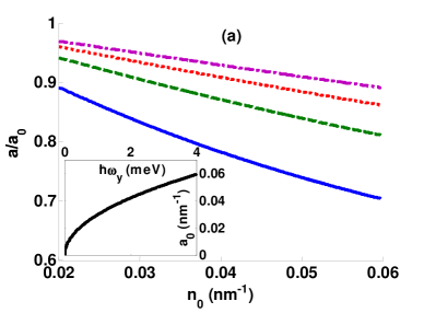
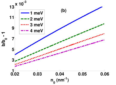
Figure 3: (Color online) (a) $a/a_{0}$ and (b) $b/b_{0}-1$ vs. electron density $n_{0}$ for different confinement strengths $\hbar\omega_{y}$ in the wire, from $1\,\mathrm{meV}$ (solid line) to $4\,\mathrm{meV}$ (dot-dashed line), for $N_{A}=10^{14}\,\mathrm{cm^{-3}}$, at $T=0$. Inset in (a): $a_{0}$ vs. $\hbar\omega_{y}$. For (b), $b_{0}=0.190\,\mathrm{nm^{-1}}$.

Meanwhile, if exchange effects are included, the zero-temperature solution for $n_{0}$ (written in terms of $k_{F}=\pi n_{0}/2$) is given by the solution of:

$$E_{F}=\frac{\hbar^{2}k_{F}^{2}}{2m^{*}}+U_{\mathrm{eff}}=\frac{\hbar^{2}k_{F}^{2}}{2m^{*}}+U_{x}+E_{yz}\\ +\frac{q^{2}}{32\pi^{2}\epsilon}\left[4k_{F}\zeta_{ab}\left(0\right)-\int_{0}^{2k_{F}}\mathrm{d}k_{x}\,\zeta_{ab}\left(k_{x}\right)\right]$$ (19)

For very small $k_{F}$, the integral in Eq. (19) above is approximately equal to $2k_{F}\zeta_{ab}\left(0\right)$, since $\zeta_{ab}\left(k\right)=\zeta_{ab}\left(0\right)+\mathrm{O}\left(k^{2}\right)$. Therefore, in this situation, $\left\langle\hat{U}_{\mathrm{exch}}\right\rangle\approx-\frac{1}{2}\left\langle U_{\mathrm{el}}\right\rangle$ and Eq. (17) can be used to obtain an approximate solution for $n_{0}$ in the presence of the exchange interaction, provided that $\zeta_{ab}\left(0\right)$ is replaced with $\zeta_{ab}\left(0\right)/2$.

Figures 3 (a) and (b) display the variational parameters $a$ and $b$ (normalized to their values when $n_{0}=0$, $a_{0}=\sqrt{m^{*}\omega_{y}/\hbar}$ and $b_{0}\approx\left[12m^{*}q^{2}N_{A}z_{d}/\hbar^{2}\epsilon\right]^{1/3}$) versus the electron density $n_{0}$ in the wire for different confinement strengths $\hbar\omega_{y}$. Calculations are carried out using the parameters for GaAsHess, 2009: $\epsilon=12.9\epsilon_{0}$, $m^{*}=0.067m_{0}$, $E_{C}=1.52\,\mathrm{eV}$. For a wire length of a few hundred nanometers, the calculated electron densities correspond to a population that varies from a few electrons to tens of electrons in the wire.

Figure 3 shows that, as $n_{0}$ increases, $a$ decreases relative to $a_{0}$ (and the characteristic length of the wavefunction along $y$, which is proportional to $1/a$, increases). This indicates that electron-electron interactions counteract the effects of the gate-induced lateral confinement and spread out the electrons over a wider region along the $y$-axis. $a_{0}$ itself increases with increasing confinement strength, as seen in the inset of Fig. 3(a). Meanwhile, $b$ increases relative to $b_{0}$ when $n_{0}$ increases, as seen in Figure 3(b), which means that electrons are confined to a narrower region near the heterojunction interface along the $z$-axis. The variation in both parameters relative to their zero-population values is more pronounced for smaller $\hbar\omega_{y}$, but $a$ is more sensitive to changes in the electron density than $b$, e.g. for $n_{0}=5\times 10^{5}\,\mathrm{cm^{-1}}$, Figures 3(a) and (b) show that $a$ decreases by up to 25% (for $\hbar\omega_{y}=1\,\mathrm{meV}$), while $b$ goes up by 1% at most for the same confinement strength. The small variation of $b$, coupled with the fact that $1/b$ (the characteristic length of the wavefunction along $z$) is of the order of a few nanometers and an order of magnitude smaller than $1/a$, is consistent with the quasi-2DEG nature of the electron layer in GaAs.

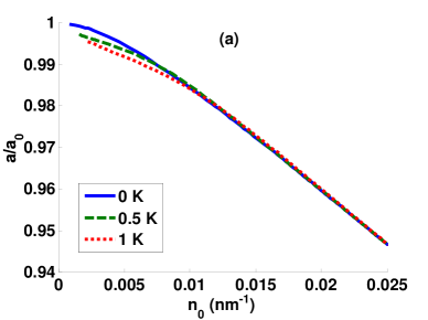
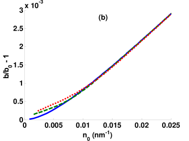
Figure 4: (Color online) (a) $a/a_{0}$ and (b) $b/b_{0}$ vs. $n_{0}$ for different temperatures, with $\hbar\omega_{y}=2\,\mathrm{meV}$ and $N_{A}=10^{14}\,\mathrm{cm^{-3}}$. $a_{0}=0.0419\,\mathrm{nm^{-1}}$ and $b_{0}=0.190\,\mathrm{nm^{-1}}$.

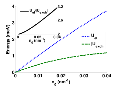
Figure 5: (Color online) Hartree and exchange terms, $U_{\mathrm{el}}$ and $U_{\mathrm{exch}}$, versus $n_{0}$ in a wire at $T=0$. $\hbar\omega_{y}=2\,\mathrm{meV}$ and $N_{A}=10^{14}\,\mathrm{cm^{-3}}$. Inset: $U_{\mathrm{el}}/\left|U_{\mathrm{exch}}\right|$ vs. $n_{0}$.

Figures 4 (a) and (b) show the temperature dependence of $a$ and $b$. Even at $1\,\mathrm{K}$, $a$ and $b$ do not vary significantly when compared to their zero-temperature values. The largest variations occur for very low electron densities, with $a$ varying by less than 0.5% (respect to its zero-temperature value) and $b$ by less than 0.05%. For high electron densities, the effect of temperature on the variational parameters is negligible.

Figure 5 displays the variation of the Hartree and exchange terms versus the electron density $n_{0}$ in the wire. As suggested by Eq. (13c), the Hartree term $U_{\mathrm{el}}$ grows approximately linearly with respect to $n_{0}$. Deviations from linearity are due to the fact that both $a$ and $b$ depend on $n_{0}$. The exchange term $\left|U_{\mathrm{exch}}\right|$ grows at a slower rate than $U_{\mathrm{el}}$ with increasing $n_{0}$. For low concentrations, $\left|U_{\mathrm{exch}}\right|$ is equal to one-half of $U_{\mathrm{el}}$, as predicted by Eq. (19).

IV Transport model for the QPC

When these results are extended to a QPC of finite length, $U_{x}$ does not take a constant value anymore, but rather depends on $x$. Additionally, the lateral confinement $U_{\mathrm{well}}$ will now drop to zero as $x$ increases. Thus, the Schrödinger equation (Eq. (1)) is no longer separable. However, if $U_{x}$ varies smoothly and slowly relative to $U_{\mathrm{well}}$ and $U_{A}$, an adiabatic approximation can be carried out in Eq. (1) to find local energy levels $E\left(k_{x};x\right)$, a local electron density $n_{0}\left(x\right)$ and $x$-dependent parameters $a$ and $b$.

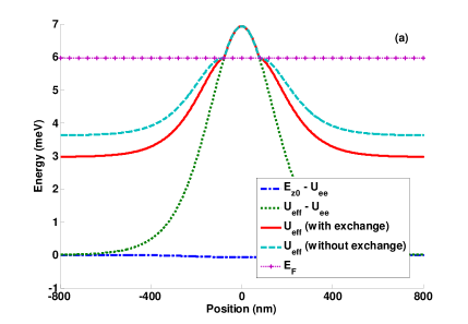
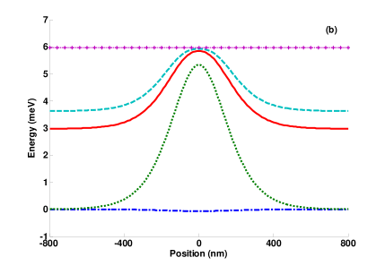
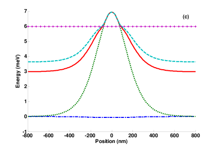
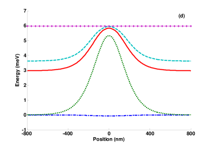
Figure 6: (Color online) Effective potential vs. position when: (a), (c) $U_{\mathrm{eff,max}}>E_{F}$ ($U_{0}=7\,\mathrm{meV}$); (b), (d) $U_{\mathrm{eff,max}}<E_{F}$ ($U_{0}=5.4\,\mathrm{meV}$). For (a) and (b), $T=0\,\mathrm{K}$; for (c) and (d), $T=1\,\mathrm{K}$. $\hbar\omega_{y,\mathrm{max}}=2\,\mathrm{meV}$, $N_{A}=10^{14}\,\mathrm{cm^{-3}}$, $n_{2D}=8.4\times 10^{10}\,\mathrm{cm^{-2}}$ and $x_{0}=200\,\mathrm{nm}$. All energies are measured with respect to $\left(E_{z0}-U_{\mathrm{ee}}\right)_{x\rightarrow-\infty}$.

Initially, we set $U_{x}\left(x\right)=U_{0}\textnormal{sech}^{2}\left(x/x_{0}\right)$, with $x_{0}$ growing as the length of the QPC increases, while the QPC barrier height $U_{0}$ is taller when the gate voltage is more negative. Ballistic transport occurs for $x_{0}$ of the order of a few hundred nanometers, given that the mean free path is of the order of several micronsWharam et al., 1988; van Wees et al., 1988. Given that the confinement length in the $y$-direction ($1/a$) is of the order of a few tens of nanometers, the adiabatic approximation remains valid for $x_{0}\gtrsim 100\,\mathrm{nm}$. Meanwhile, the lateral confinement becomes $U_{\mathrm{well}}\left(x,y\right)=m^{*}\left[\omega_{y}\left(x\right)\right]^{2}y^{2}/2$, where we assume $\omega_{y}\left(x\right)=\omega_{y,\mathrm{max}}\sqrt{U_{x}\left(x\right)/U_{0}}$. Once the effective potential $U_{\mathrm{eff}}\left(x,k_{x}\left(x\right)\right)$ (Eq. (10)) is found for sample points along the $x$-axis, the transmission coefficient $\mathrm{T}\left(E\left(k_{x},\sigma\right)\right)=\mathrm{T}_{\sigma}\left(E\right)$ is calculated by the transfer matrix methodJonsson and Eng, 1990. Finally, the conductance is obtained using the Landauer formulaDatta, 1997,

$$G=\frac{e^{2}}{h}\sum_{\sigma}\int\mathrm{d}E\,\left(-\frac{\partial f_{T}}{\partial E}\right)\mathrm{T}_{\sigma}\left(E\right)$$ (20)

The Fermi level $E_{F}$ is determined by the electron density $n_{2D}$ in the 2DEG far away from the QPC, where the effective potential is $U_{\mathrm{eff}}\left(x\rightarrow-\infty\right)=\left\langle\hat{T}_{z}\right\rangle+\left\langle U_{A}\right\rangle+U_{\mathrm{ee}}=E_{z0}\left(x\rightarrow-\infty\right)$:

$$E_{F}-U_{\mathrm{eff}\left(x\rightarrow-\infty\right)}=\frac{\pi\hbar^{2}n_{2D}}{m^{*}}$$ (21)

Of particular interest is the case of a very low carrier concentration in the QPC. Then, the effective potential, and therefore the transmission coefficient, depends on whether or not one of the electrons shares the same spin with the electron preceding it on the wire. If the electron spins are different, then the exchange term in the effective potential drops out and the interaction is anti-ferromagnetic.

V Results and discussion

Figures 6(a)-(d) show the profile of the effective potential $U_{\mathrm{eff}}\left(E=E_{F}\right)$ at $T=0$ along the $x$-direction when the maximum value of the effective potential, $U_{\mathrm{eff,max}}$ is, respectively, (a) greater than or (b) less than $E_{F}$. Here we assume that $n_{2D}=8.4\times 10^{10}\,\mathrm{cm^{-2}}$, so that for $x\rightarrow-\infty$ the Fermi energy is $3\,\mathrm{meV}$ above $U_{\mathrm{eff}}$, according to Eq. (21). Energies in the plot are measured relative to $\left(E_{z0}-U_{\mathrm{ee}}\right)_{x\rightarrow-\infty}$. The solid and dashed lines represent the effective potential when the exchange interaction is either included or ignored. The separation between the dotted and solid (or dashed) lines corresponds to the contribution of electron-electron interactions, $U_{\mathrm{ee}}$, to $U_{\mathrm{eff}}$, which is more significant far away from the QPC (i.e. where the QPC barrier height, $U_{x}$, drops to zero).

As $U_{x}$ increases near $x=0$, $U_{\mathrm{ee}}$ becomes smaller because fewer electron states are populated, and therefore $U_{\mathrm{eff}}$ increases less rapidly. In particular, when $U_{\mathrm{eff}}>E_{F}$, the electron channel is depleted and $U_{\mathrm{ee}}=0$. Figure 6 shows that, at the point where $U_{\mathrm{eff}}=E_{F}$, there is a kink or shoulder in the effective potential due to the onset of Coulomb interactions in $U_{\mathrm{eff}}$. Above $E_{F}$, $U_{\mathrm{eff}}$ varies at the same rate as $U_{x}$. The kink is not present in Figure 6(b), since the effective potential in that figure is below $E_{F}$ throughout the QPC, but $U_{\mathrm{ee}}$ is still smaller near the center of the QPC when compared to points that are farther away.

Figures 6(c) and (d) show the same plots for $T=1\,\mathrm{K}$. The kink in the effective potential is less pronounced in Fig. 6(c) compared to Fig. 6(a) because the electron concentration does not vanish anymore when $U_{\mathrm{eff}}>E_{F}$, and therefore the Hartree and exchange terms contribute to the effective potential, especially when $U_{\mathrm{eff}}$ is still very close to $E_{F}$. Far away from the QPC, the potential profiles are indistinguishable from their zero-temperature counterparts.

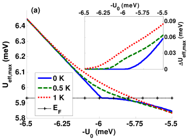
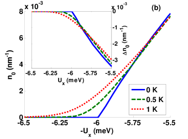
Figure 7: (Color online) (a) Maximum effective potential vs. $U_{0}$, including exchange effects, for different temperatures. Inset: $\Delta U_{\mathrm{eff,max}}=U_{\mathrm{eff,max}}\left(\textnormal{w/o exchange}\right)-U_{\mathrm{eff,max}}\left(\textnormal{w/exchange}\right)$ vs. $U_{0}$. (b) Electron density vs. $U_{x}$, including exchange effects, for different temperatures. Inset: $\Delta n_{0}=n_{0}\left(\textnormal{w/o exchange}\right)-n_{0}\left(\textnormal{w/exchange}\right)$. All parameters (except temperature) as in Figure 6.

In Figure 7 we plot $U_{\mathrm{eff,max}}$ versus the maximum QPC barrier height ($U_{0}$) for different temperatures. At zero temperature, the effective potential maximum decreases linearly with $U_{0}$ above the Fermi energy, i.e. when the QPC is “pinched-off” and there are no electrons in the 1D channel. When $U_{\mathrm{eff,max}}$ crosses the Fermi level at $U_{0}\approx 6\,\mathrm{meV}$, it remains practically constant (“pinned”) over a certain range of $U_{0}$ values while the channel opens. Then, it decreases at a slow rate for $U_{0}\lesssim 5.75\,\mathrm{meV}$, when the QPC channel becomes more populated with electrons. This pinning effect is a consequence of the compressibility peak in the 1D electron gas, in agreement with previous works*[][.Wenotice; however; thatthegeometryoftheconstrictionisdifferentfromthesingleQPCconsideredinouranalysis.Additionally; theeffectivepotentialinthatpaperreferstothepotentialofthedetectorgateandhasadifferentmeaningthaninthepresentwork; inwhich$U_eff$wasdefinedasthe1Dpotentialprofilealongtheconstriction.]Luscher2007; Hirose et al. (2001); Ihnatsenka and Zozoulenko (2009). It also occurs when $U_{\mathrm{eff}}$ crosses the Fermi level on both sides of the QPC when the 1D channel is still closed, and is responsible for the “kink” observed in the barrier profile (Fig. 6(a)). The pinning is less effective at non-zero temperatures because the electron density in the QPC is not zero. The dependence of $n_{0}$ on $U_{x}$ is shown in Figure 7(b). As predicted by Eq. (17), decreasing $U_{x}$ past the critical point at $U_{x}\approx 6\,\mathrm{meV}$ leads to an increase in $n_{0}$. Meanwhile, $n_{0}$ increases with rising temperature near the effective potential crossover, as expected.

The changes in $U_{\mathrm{eff,max}}$ and $n_{0}$ when exchange effects are neglected are shown in the insets of Figures 7(a) and (b). As can be seen in Fig. 7(a), neglecting the (negative) exchange term leads to an increase in the maximum effective potential below $E_{F}$, as explained in the comments of Fig. 6. In addition, $U_{\mathrm{eff,max}}$ also becomes less sensitive to variations in $U_{0}$, which indicates that the pinning of the effective potential is enhanced by the absence of the exchange interaction. The increase in $U_{\mathrm{eff,max}}$ becomes even more pronounced when temperature is increased. Since the effective potential is higher, the carrier concentration in the absence of exchange effects is lower relative to the case with exchange, as shown in the inset of Fig. 7(b).

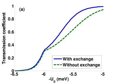
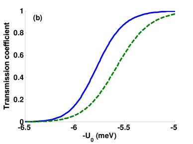
Figure 8: (Color online) Transmission coefficient vs. $U_{0}$ for (a) $T=0\,\mathrm{K}$; (b) $T=1\,\mathrm{K}$, showing the curves in the presence and in the absence of the exchange interaction. All other parameters as in Figure 6.

A plot of the transmission coefficient as a function of $U_{0}$ at $T=0$ (Figure 8(a)) reveals a kink or anomaly close to 0.35, when $U_{0}$ reaches the critical point of $\sim 6\,\mathrm{meV}$ and $U_{\mathrm{eff,max}}$ crosses $E_{F}$. This kink is a consequence of the pinning of the effective potential just below $E_{F}$ and is more pronounced when the exchange interaction is neglected (dashed curve) since the effective potential is enhanced, as mentioned in our discussion of the insets in Figs. 6 and 7. In Figure 8(b), we display the transmission coefficient at $T=1\,\mathrm{K}$ and show that the anomaly disappears with increasing temperature. This is caused by the thermal smearing of the effective potential pinning, as shown in Fig. 7. At zero temperature, when the gate voltage is sufficiently negative, the transmission coefficient drops rapidly because of the sudden increase in the height $U_{\mathrm{eff,max}}$ of the effective potential (Figures 7(a) and (c)). However, due to the modulation of the potential barrier with increasing temperature, the changes in $U_{\mathrm{eff,max}}$ are smoother and the transmission coefficient does not change as abruptly, thus softening the anomaly. By neglecting the (negative) exchange interaction (dashed curve), the effective potential barrier is taller, thereby resulting in a lower transmission coefficient, as can be seen both in Figure 8(a) (for $U_{0}$ below the critical value of $6\,\mathrm{meV}$) and 8(b).

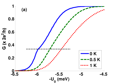
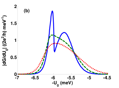
Figure 9: (Color online) (a) Conductance vs. $U_{0}$ for different temperatures. For clarity, each successive curve is shifted to the right by $0.25\,\mathrm{meV}$. The dot-dashed line indicates the location of the kink. (b) Slope of the conductance, $\left|dG/dU_{0}\right|$, vs. $U_{0}$. Exchange effects are included. All parameters as in Figure 6.

Figure 9(a) shows the QPC conductance as a function of $U_{0}$ for different temperatures. Here we included exchange effects on the barrier. At $T=0\,\mathrm{K}$, the kink in the transmission coefficient at $G\sim 0.35G_{0}$ is well reproduced in the conductance, but is smeared out as temperature increases, even by a few tenths of a kelvin. This thermal smearing is confirmed in Figure 9(b), where we plot the slope of the conductance as a function of $U_{0}$. At $T=0\,\mathrm{K}$, the conductance slope exhibits a double peak with a sharp maximum before $U_{0}=6\,\mathrm{meV}$, followed by a broader and lower maximum, which indicates that the kink in the conductance is not simply a slope change, but is rather due to the onset of the 1D compressibility of the electron gas. However, as temperature increases the dip in the double peak structure disappears to leave a single and broad peak.

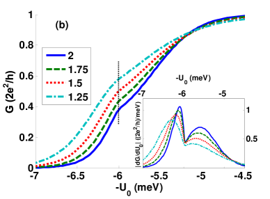
Figure 10: (Color online) (a) Conductance at $T=0$ vs. $U_{0}$ for: (a) $U_{x}=U_{0}\textnormal{sech}^{2}\left(x/x_{0}\right)$, for different $x_{0}$; (b) $U_{x}=U_{0}\left[1+\left(x/x_{0}\right)^{N}\right]^{-1}$, for different $N$. Exchange effects are included. All parameters (apart from $x_{0}$ in (a)) are the same as in Figure 6. The thin vertical dotted line shows the location of the kink. Insets: slope of the conductance vs. $U_{0}$.

In Figure 10(a), we display the sensitivity of the $T=0\,\mathrm{K}$ conductance as a function of the QPC length, which consists in varying $x_{0}$, the characteristic length of the potential barrier (defined as $U_{x}=U_{0}\textnormal{sech}^{2}\left(x/x_{0}\right)$). As can be seen, a decrease in $x_{0}$, corresponding to a shorter QPC, leads to a spread of the conductance with a lower slope over a broader $U_{0}$ potential range, and shifts the kink anomaly upwards, towards $G\sim 0.4G_{0}$. At the same time, the kink becomes softer and broader (Fig. 10(a), inset). This upward displacement of the kink is caused by the narrower barrier for which the transmission is enhanced at low energy compared to the conductance in longer QPCs. A more dramatic effect on the conductance is observed if the $U_{x}$-potential profile changes. In Figure 10(b), we use a barrier potential of the form $U_{x}=U_{0}\left[1+\left(x/x_{0}\right)^{N}\right]^{-1}$ (where $N$ is a positive exponent) to calculate the QPC conductance at $T=0\,\mathrm{K}$. Compared to the $\textnormal{sech}^{2}\left(x\right)$ potential shape, this function has a sharper drop at $x=0$ and a longer tail for $x>x_{0}$, especially when $N$ is small. As can be seen, a decrease in the value of the exponent $N$ leads to an upwards displacement of the anomaly since for $N=2$ the anomaly occurs at $G\sim 0.4G_{0}$, whereas for $N=1.25$ it rises up to $G\sim 0.6G_{0}$. The transmission is higher in this case compared to higher-$N$ potentials over the whole $U_{0}$ energy range. At the same time, the anomaly broadens and shifts to lower $U_{0}$ potential values (Fig. 10(b), inset).

VI Conclusions

We developed a 3D quantum mechanical model for near-equilibrium ballistic transport through a constriction in a 2D GaAs/AlGaAs electron gas by using a self-consistent variational approach. We were able to define an effective 1D potential ($U_{\mathrm{eff}}$) for the constriction, which takes into account the static potential arising from fixed acceptor charges, many-body effects, and the confinement and barrier potentials. Away from the constriction, the model reduces to that of a 2DEG with a fixed Fermi level. In the constriction, the gate-induced potential leads to a downward shift of the 2DEG subbands. Our model, based on a transmission matrix technique, predicts an anomaly in the range $0.3G_{0}<G<0.6G_{0}$, during the rise to the first conductance plateau at $T=0\,\mathrm{K}$. This anomaly is caused by a change of slope in the variation of the effective potential with the external gate voltage due to the charging of the 1D channel at the compressibility peak, in agreement with previous observationsLüscher et al., 2007; Hirose et al., 2001; Ihnatsenka and Zozoulenko, 2009. Our model also predicts an anomaly enhancement in the case of anti-ferromagnetic interaction in the QPC as the attractive exchange interaction lowers the potential barrier, thereby disqualifying the presence of any spontaneous spin polarization. Our main result, however, is that the exact conductance value for the anomaly depends on the length of the QPC and the shape of the potential barrier, i.e. long QPCs make the conductance sharper, while sharper potentials lead to a higher value of the conductance kink. These findings tend to be in agreement with experimental observations that show a shift of the 0.7 plateau toward higher conductance values under higher source–drain biasesCronenwett et al., 2002, which also sharpens the QPC potential. However, our self-consistent model also shows the barrier sensitivity to temperature that smears out the anomaly, unlike the enhancement of the 0.7 feature with increasing temperature that is observed experimentallyThomas et al., 1996; Nuttinck et al., 2000; Cronenwett et al., 2002. We believe this result is due to the approximation of a smooth QPC barrier, which may not well reproduce the potential landscape characterized by the AlGaAs substitutional disorder at the GaAs/AlGaAs interfaceThean et al., 1997, nor any possible bound states required for the occurrence of a Kondo-like effectCronenwett et al., 2002; Rejec and Meir, 2006. These issues, as well as the investigation of far-from-equilibrium transport in QPCs, will be the subject of a forthcoming paper.