Formation of Stable Magnetars from Binary Neutron Star Mergers

Abstract

By performing fully general relativistic magnetohydrodynamic simulations of binary neutron star mergers, we investigate the possibility that the end result of the merger is a stable magnetar. In particular, we show that, for a binary composed of two equal-mass neutron stars (NSs) of gravitational mass $M\sim 1.2M_{\odot}$ and equation of state similar to Shen et al. at high densities, the merger product is a stable NS. Such NS is found to be differentially rotating and ultraspinning with spin parameter $J/M^{2}\sim 0.86$, where $J$ is its total angular momentum, and it is surrounded by a disk of $\approx 0.1M_{\odot}$. While in our global simulations the magnetic field is amplified by about two orders of magnitude, local simulations have shown that hydrodynamic instabilities and the onset of the magnetorotational instability could further increase the magnetic field strength up to magnetar levels. This leads to the interesting possibility that, for some NS mergers, a stable and magnetized NS surrounded by an accretion disk could be formed. We discuss the impact of these new results for the emission of electromagnetic counterparts of gravitational wave signals and for the central engine of short gamma-ray bursts.

1. Introduction

Binary neutron stars (BNSs) are the leading candidates for the central engine of short gamma-ray bursts (SGRBs; Blinnikov et al. 1984; Paczynski 1986; Eichler et al. 1989). They are also one of the most powerful sources of gravitational waves (GWs), and advanced interferometric detectors are expected to observe these sources at rates of $\sim 0.4-400$ events per year (Abadie et al., 2010).

Fully general-relativistic simulations have shown how such mergers can lead to the formation of hypermassive neutron stars (HMNSs), i.e., of NSs with masses larger than the maximum mass that can be supported by uniform rotation. Due to loss of angular momentum via GW emission and magnetic fields, the HMNS eventually collapses in less than $\sim 1\,{\rm s}$ to a black hole (BH) surrounded by an accretion disk (Baiotti et al., 2008; Kiuchi et al., 2009; Giacomazzo et al., 2011a; Faber & Rasio, 2012). When magnetic fields are present, they can provide a mechanism to extract energy from the BH and disk, and power collimated relativistic jets (Rezzolla et al., 2011).

A source of uncertainty in BNS simulations is due to the lack of detailed knowledge of the equation of state (EOS) of NSs (see Hebeler et al. 2013 for a recent discussion of EOSs). Current observations have shown that NSs with masses of $\sim 2M_{\odot}$ exist (Demorest et al., 2010; Antoniadis et al., 2013), and therefore the NS EOS must support a mass at least as large as that. This opens the interesting possibility that the merger of BNSs could produce not only HMNSs, but also NSs which are stable against gravitational collapse. This possibility has interesting applications for observations of SGRBs (Dai et al., 2006; Belczynski et al., 2008; Rowlinson et al., 2013), as well as for the possible emission of long periodic GW signals (Dall’Osso et al., 2009) and their electromagnetic counterparts (Zhang, 2013; Gao et al., 2013; Fan et al., 2013). In particular, Rowlinson et al. (2013) found that several of the SGRBs that show a plateau phase in the X-ray lightcurve may be explained with the formation of a stable magnetar after the BNS merger. X-ray lightcurves indeed suggest a long-lived central engine (Margutti et al., 2011), which is hard to explain if all the BNS mergers produce an HMNS which collapses to a BH in less than $\sim 1{\rm s}$; the remnant torus is also expected to be completely accreted on the same timescale (Rezzolla et al., 2011), unless magnetic or gravitational instabilities set in (Proga & Zhang, 2006; Perna et al., 2006). The formation of a stable magnetar could also explain the extended emission observed in several SGRBs (Metzger et al., 2008).

In this Letter we investigate, for the first time and in fully general-relativistic MHD, the regime in which BNSs may lead to the formation of a stable NS. By considering models with and without magnetic fields, and by performing the longest (to date) general relativistic simulations of magnetized BNS mergers, we show that stable magnetized NSs can indeed be formed for some range of masses, and we discuss the implications of these new results for the electromagnetic signals that they may emit. Note that the formation of a stable magnetar is a non-trivial outcome; in fact, even if the total mass of a BNS system is below the maximum mass, collapse to BH may still happen if the central density of the merger product is above a certain value (depending on the EOS). NSs with masses below the maximum mass can indeed collapse to BHs (e.g., model D0 in Baiotti et al. 2007), and the stability properties of NSs are defined by both their masses and central densities (Friedman et al., 1988). In this Letter, together with presenting the first simulation of the formation of a stable NS from a binary merger, we also discuss the NS final spin, the formation of a disk, magnetic field amplification, the GW signal, and possible electromagnetic counterparts.

Table 1Initial Data

Binary	$\rho_{\rm max}~{}({\rm g\,cm^{-3}})$	$M^{\infty}_{1,2}~{}(M_{\odot})$	${\cal C}^{\infty}_{1,2}$	$d/M_{\rm ADM}$	$M_{\rm ADM}~{}(M_{\odot})$	$J~{}({\rm g}\,{\rm cm}^{2}\,{\rm s}^{-1})$	$\Omega_{0}~{}({\rm rad\,ms^{-1}})$	$B_{0}~{}({\rm G})$
B0	$4.40\times 10^{14}$	$1.22$	$0.13$	$15.6$	$2.42$	$5.42\times 10^{49}$	$1.70$	$0$
B12	$4.40\times 10^{14}$	$1.22$	$0.13$	$15.6$	$2.42$	$5.42\times 10^{49}$	$1.70$	$1.0\times 10^{12}$

Section 2 details our numerical methods and the initial models. Section 3 describes evolution and dynamics of these systems, while in Section 4 we discuss their gravitational and electromagnetic signals. Section 5 summarizes our main results. For convenience, we use a system of units in which $c=G=M_{\odot}=1$, unless explicitly stated otherwise.

2. Numerical Methods and Initial Data

The simulations presented here were performed using the publicly available Einstein Toolkit (Löffler et al., 2012), coupled with our fully general relativistic MHD code Whisky (Giacomazzo & Rezzolla, 2007; Giacomazzo et al., 2011a). Details about the numerical methods can be found in Giacomazzo et al. (2011a), except that in our work the spacetime evolution is obtained using the McLachlan code (Löffler et al., 2012), and Whisky now implements the modified Lorenz gauge to evolve the vector potential and the magnetic field (Farris et al., 2012). The simulations presented here use adaptive mesh refinement with six refinement levels; the finest grid covers completely each of the NSs during the inspiral and merger, while the coarsest grid extends up to $\sim 777\,{\rm km}$. Our fiducial runs have a resolution of $\sim 225\,{\rm m}$ on the finest grid, but convergence tests have been performed using both a coarser ($\sim 360\,{\rm m}$) and a finer resolution ($\sim 180\,{\rm m}$).

The initial data were produced using the publicly available code LORENE (Taniguchi & Gourgoulhon, 2002). The initial solutions for the binaries were obtained assuming a quasi-circular orbit, an irrotational fluid-velocity field, and a conformally-flat spatial metric. The matter is modeled using a polytropic EOS $p=K\rho^{\Gamma}$, where $p$ is the pressure, $\rho$ the rest-mass density, $K=30000$ and $\Gamma=2.75$, in which case the maximum gravitational mass is $M\simeq 2.43\,M_{\odot}$ for a non-rotating NS, and $M\simeq 2.95\,M_{\odot}$ for a uniformly maximally-rotating star, in agreement with recent observations of NS masses (Demorest et al., 2010; Antoniadis et al., 2013). An ideal-fluid EOS with $\Gamma=2.75$ is used during the evolution in order to allow for shock heating during merger. This EOS has been chosen since it fits very well the Shen nuclear EOS (Shen et al., 1998a, b) at high densities (Oechslin et al., 2007), and hence it provides a more accurate description of the evolution of the plasma in the high-density regions than the simpler $\Gamma=2$ polytrope used in our previous simulations (Giacomazzo et al., 2009, 2011a; Rezzolla et al., 2011). In this work we consider an equal-mass system both with and without a magnetic field, and with a total gravitational mass $M_{\rm ADM}=2.42M_{\odot}$. When a magnetic field is present, its initial configuration is purely poloidal and aligned with the angular momentum of the binary as in Giacomazzo et al. (2011a). Details about the initial configurations are provided in Table 1.

3. Dynamics

We first evolved the unmagnetized case (model B0) with three different resolutions: $h=0.24M_{\odot}\sim 360\,{\rm m}$ (low), $h=0.15M_{\odot}\sim 225\,{\rm m}$ (medium), and $h=0.12M_{\odot}\sim 180\,{\rm m}$ (high). In all cases, the binary inspirals for five orbits before merging. The main aspects of the dynamics are illustrated in Figure 1, where we show the rest-mass density on the equatorial plane for the high resolution case. One important point to note is that, as observed in previous simulations of BNS mergers, the compact object that is formed after the inspiral is differentially rotating. However, while in previous simulations it was an HMNS, in the current simulations the NS is well below that limit ($M\simeq 2.95\,M_{\odot}$ for our EOS), and hence it does not collapse to BH. At the end of our simulation, the differentially-rotating NS has a mass $M\sim 2.36M_{\odot}$ and is surrounded by a disk of $\approx 0.1M_{\odot}$.

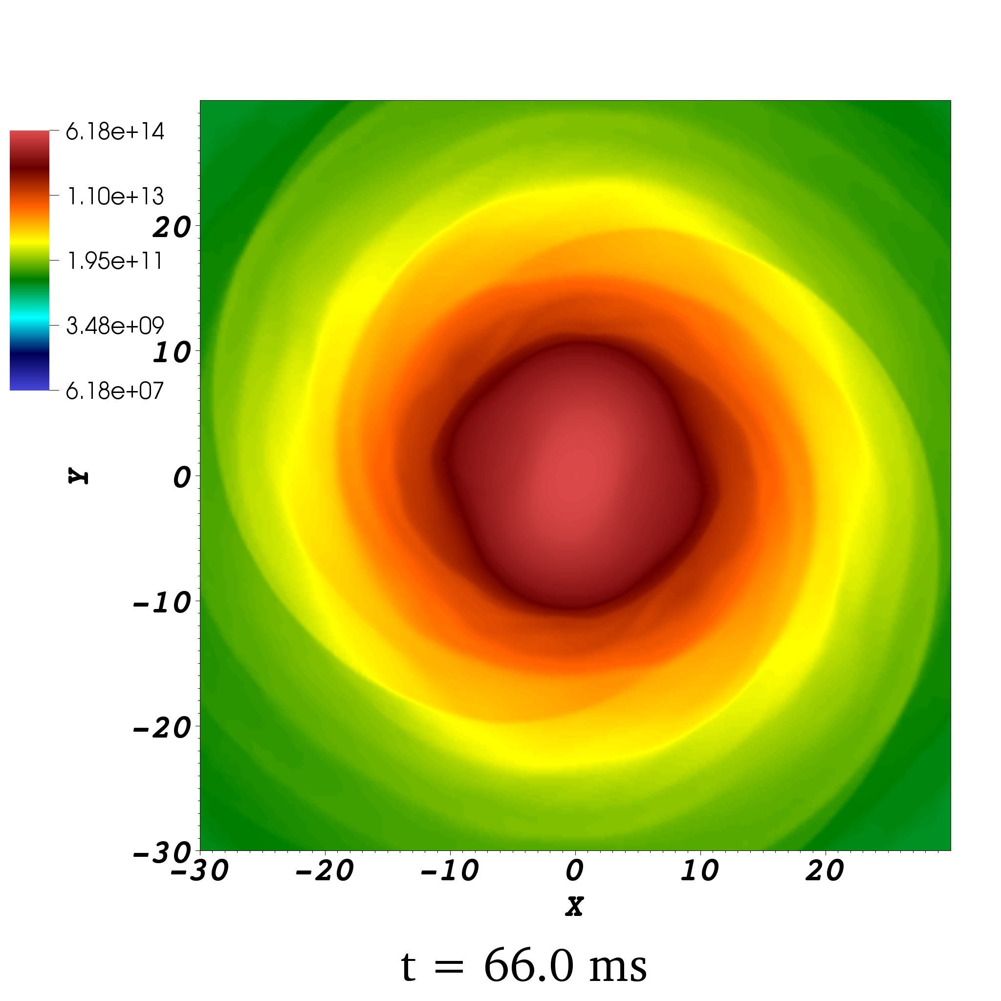
Figure 1.— Evolution of the rest-mass density in ${\rm g\,cm^{-3}}$ on the equatorial plane for model B0 evolved with the highest resolution ($h\sim 180{\rm m}$). The different panels show respectively the initial conditions ($t=0$), the inspiral, the time of the merger ($t\sim 15\,{\rm ms}$), the post-merger phase, and the formation of the “ultraspinning” NS (last two panels). The units of distance are $M_{\odot}\sim 1.5\,{\rm km}$ and the time in ${\rm ms}$ is reported at the bottom of each panel.

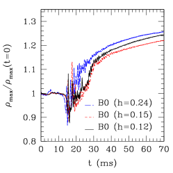
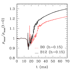
Figure 2.— Top left panel: evolution of the maximum of the rest-mass density $\rho$ normalized to its initial value for model B0 evolved with three different resolutions. The blue long-dashed line refer to $h=0.24M_{\odot}\sim 360\,{\rm m}$, the red short-dashed line to $h=0.15M_{\odot}\sim 225\,{\rm m}$, and the black solid line to $h=0.12M_{\odot}\sim 180\,{\rm m}$. Top right panel: same quantity as in the left panel, but for models B0 (red short-dashed line) and B12 (black solid line) evolved with our fiducial resolution ($h=0.15M_{\odot}\sim 225\,{\rm m}$). Bottom left panel: evolution of the maximum of the magnetic field for model B12. The black solid line shows the maximum of the total magnetic field, the blue dotted line the maximum of its poloidal component, and the red dashed line the maximum of its toroidal component. Bottom right panel: evolution of the total magnetic energy as a function of time. In the last two panels the vertical dashed line shows the time of the merger of the two NS cores.

This can also be seen in the top left panel of Figure 2, where we show the evolution of the maximum of the rest-mass density normalized to its initial value for the three resolutions. Following an initial transient after the merger at $t\sim 15\,{\rm ms}$, when the rest mass density increases by $\sim 15\%$ due to the compression of the NS cores, the rate of the rest-mass increase diminishes, and the central density approaches a finite value. Simulations of unstable HMNSs, on the other hand, show a clear increase in the rest-mass density (see, e.g., the left panel of Figure A1 in Rezzolla et al. 2010).

Since these objects are differentially rotating NSs, it is interesting to further explore what happens when magnetic fields are added to the simulation, as they may redistribute angular momentum (Giacomazzo et al., 2011a). The top right panel of Figure 2 shows a comparison between the evolution of the maximum of the rest-mass density for models B0 and B12. While model B12 shows a larger increase after the merger, due to redistribution of angular momentum by the magnetic field, its maximum density is also converging toward a constant value. In the bottom left panel of Figure 2, we show the evolution of the maximum of the magnetic field for model B12. As already observed in our previous simulations (Giacomazzo et al., 2011a), the magnetic field grows by one order of magnitude during the merger because of hydrodynamic instabilities such as the Kelvin-Helmholtz (KH; see also Price & Rosswog 2006; Baiotti et al. 2008), and because of compression of the cores. The KH also causes an increase of the toroidal component of the magnetic field. This component is further amplified by magnetic winding due to differential rotation. The amplification of the magnetic field can also be observed in the bottom right panel of Figure 2, where we show the total magnetic energy $E_{\rm MHD}$ as a function of time. At the end of the simulation, $E_{\rm MHD}\sim 10^{44}\,{\rm erg}$, but the $E_{\rm MHD}(t)$ slope suggests that further growth is expected if the simulation were continued for a longer time. We also note that local simulations show that the KH instability can further amplify the magnetic field up to $\sim 10^{16}{\rm G}$, i.e, well into magnetar levels (Zrake & MacFadyen, 2013). Unfortunately, the resolutions required to correctly resolve such small scale dynamics and other instabilities, such as the magnetorotational instability (MRI), are far above what can be obtained in these global simulations. We also note that differential rotation can cause a further increase of the magnetic field at later times (Thompson & Duncan, 1993) and hence magnetar field levels could be reached via several mechanisms.

For a clearer interpretation of our results, in Figure 3 we show equilibrium curves for uniformly rotating NSs. The two black solid lines show non-rotating and maximally-rotating NSs that are stable against gravitational collapse, while the two red-dashed lines straddle the region of uniformly rotating models which are unstable. NSs with densities larger than $\sim 1.2\times 10^{15}\,{\rm g\,cm^{-3}}$ are unstable and collapse to BHs (this is true also for differentially rotating NSs, see Giacomazzo et al. 2011b). The filled blue circle shows the position of the two NSs composing our binary, while the blue square indicates the position of the NS produced by the merger at the end of the simulation, for model B0 at medium resolution. First, as mentioned before, its mass and central density are lower than the maximum value for a stable uniformly-rotating NS, hence it does not form an HMNS. This object is differentially rotating with spin parameter $J/M^{2}\sim 0.86$; its total angular momentum $J$ is higher, by a factor $J/J_{\rm max}\sim 1.11$, than the maximum angular momentum $J_{\rm max}$ which can be obtained for a rigidly rotating NS with the same rest mass. This is why it is located above the top black curve.

Duez et al. (2006) studied the evolution of several stable differentially rotating and magnetized NS models in two dimensions and at much higher resolutions than what can be afforded in three-dimensional simulations of BNS mergers. One of their models, which they call “ultraspinning”, is very similar to the end product of our BNS merger simulations. In particular, Duez et al. (2006) studied the impact of the magnetic field on the long-term evolution of this model. Their simulations showed an amplification of the magnetic field due to the onset of the MRI instability, and found that the final configuration was an uniformly rotating NS surrounded by a differentially rotating and magnetized disk.

4. Gravitational Waves and Short Gamma-Ray Bursts

Here we discuss the impact of our simulations for the detection of GW signals, as well as for the possible connection with current observations of SGRBs.

Figure 4 shows the amplitude of the $l=2,m=2$ mode of the GW signal for our models B0 and B12, run at medium resolution. As already observed in Giacomazzo et al. (2009) and in Giacomazzo et al. (2011a), the magnetic field does not have an impact on the inspiral, but it affects the signal after the merger. In particular, due to the slightly larger compactness of the magnetized NS, the GW signal is slightly larger in amplitude.

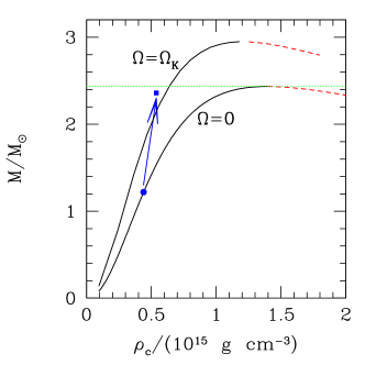
Figure 3.— The gravitational mass of an NS as a function of the central value of its rest-mass density $\rho_{c}$. The solid and dashed lines represent equilibrium solutions for uniformly rotating NSs. The bottom black solid line refers to stable non-rotating NSs (i.e, TOVs), while the bottom red dashed line to gravitationally unstable non-rotating NSs (note that they have masses below the maximum mass). The top black-solid and red-dashed lines refer respectively to stable and unstable NSs rotating at the mass shedding limit. Uniformly rotating NSs located in the region between the two red dashed lines are unstable and will collapse to BH. The filled blue circle shows the position of the NSs composing our binary, while the filled blue square indicates the NS formed at the end of the simulation of model B0. The horizontal green dotted line shows the maximum mass for a non-rotating NS. As one can easily see, the NS formed after the merger has a mass lower than the maximum mass for a non-rotating NS and it is located in the stable region.

As already mentioned in the previous section, long-term simulations of “ultraspinning”, magnetized, differentially rotating NSs (similar to the ones produced at the end of our BNS merger simulations) have shown that the end product of the evolution is an uniformly-rotating NS surrounded by a differentially rotating magnetized disk (Duez et al., 2006). In addition, those simulations were able to resolve the MRI and showed the formation of a mainly poloidal and collimated magnetic field aligned with the spin axis of the NS. Such a configuration could emit relativistic jets and power SGRBs (Meier et al., 2001). This possibility is especially interesting in light of the recent observations of extended emission following SGRBs (Metzger et al., 2008). An analysis of Swift-detected SGRBs by Rowlinson et al. (2013) has showed that all SGRBs with one or more breaks in their X-ray light curves display a plateau phase, which can be interpreted as the luminosity of a relativistic magnetar wind (Zhang & Mészáros, 2001; Fan & Xu, 2006; Metzger et al., 2011). Under the assumption of energy loss by pure dipole radiation, and neglecting, to first approximation, the enhanced angular momentum losses due to neutrino-driven mass loss, the duration of the plateau and its luminosity can be used to infer the magnetic field of the magnetar and its birth period. The observed range of values (plateau durations $\sim 10^{2}-10^{4}$ s, and [$1-10^{4}$ keV] luminosities $\sim 10^{46}-10^{49}$ erg s^-1) yielded typical periods on the order of a few milliseconds, and magnetic field strengths in the range $B\sim 10^{15}-10^{16}$ G. Following the initial rapidly spinning magnetar phase, two outcomes are possible, depending on how steep the post-plateau decay phase is. If the magnetar is unstable and decays to a BH, then the post plateau emission, only due to curvature radiation, fades away very quickly. On the other hand, the $\sim t^{-2}$ decay of the stable magnetar emission gives a more prolonged energy injection, and hence brighter fluxes at later times. The detailed analysis by Rowlinson et al. (2013) identified a handful of SGRBs whose late X-ray emission is consistent with that of a stable magnetar. Moreover, X-ray and optical afterglow emitted by a magnetar (Dall’Osso et al., 2011; Zhang, 2013) may not be collimated, and hence they may be observed even without a SGRB detection (Gao et al., 2013).

Figure 4.— The $l=2,m=2$ mode of the GW signal for model B0 (red dashed line) and B12 (black solid line).

Other numerical simulations of magnetized HMNSs have further demonstrated the possibility of producing outflows with energy of $\sim 10^{51}{\rm erg}$ for magnetic fields of $\sim 10^{15}{\rm G}$ (Kiuchi et al., 2012). As already discussed before, such magnetic fields can be naturally formed in our scenario via KH and MRI instabilities. According to Kiuchi et al. (2012), a magnetic field of $\sim 10^{15}{\rm G}$ could give rise to an electromagnetic emission observable in the radio band and hence provide an interesting electromagnetic counterpart to the GW signal even if a SGRB is not observed.

5. Summary

We have presented the first general relativistic magnetohydrodynamic simulations that show the possible formation of a stable magnetar. The NS formed after the merger is found to be differentially rotating and ultraspinning. Since our computational resources are not enough to fully resolve the MRI, the magnetic field is amplified by about two orders of magnitude, but further amplification is possible and indeed observed in two and three-dimensional simulations of differentially rotating NSs (Duez et al., 2006; Siegel et al., 2013). Moreover, long term evolution of such models has shown that the magnetic field can impact the angular velocity profile of the NS leading to the formation of an uniformly rotating NS surrounded by an accretion disk and with a collimated magnetic field (Duez et al., 2006). While it will be difficult to differentiate the GW signal between the magnetized and the unmagnetized scenarios, strong electromagnetic counterparts that would be suppressed in collapsing NSs could be easily produced and observed in radio (Kiuchi et al., 2012), optical (Dall’Osso et al., 2011; Zhang, 2013; Gao et al., 2013), X-rays (Rowlinson et al., 2013), and gamma-rays (Gompertz et al., 2013).

While our simulations focused on equal-mass systems, the same scenario may be produced after the merger of unequal-mass BNSs. In this case, matter ejected during the inspiral due to the tidal disruption of the less massive components, may later fall back on the magnetar and trigger its collapse to BH (Giacomazzo & Perna, 2012). More detailed observations of the early afterglow phase, as expected with the planned future mission LOFT (Amati et al., 2013), will be especially useful in discriminating among various formation scenarios. Last, simultaneous detections of GWs and SGRBs will fully unveil the mechanism behind the central engine and help constrain its properties (Giacomazzo et al., 2013).

References

- Abadie et al. (2010) Abadie, J., Abbott, B. P., Abbott, R., et al. 2010, CQGra, 27, 173001
- Amati et al. (2013) Amati, L., Del Monte, E., D’Elia, V., et al. 2013, ArXiv:1302.5276
- Antoniadis et al. (2013) Antoniadis, J., Freire, P. C. C., Wex, N., et al. 2013, Sci, 340, 448
- Baiotti et al. (2008) Baiotti, L., Giacomazzo, B., & Rezzolla, L. 2008, Phys. Rev. D, 78, 084033
- Baiotti et al. (2007) Baiotti, L., Hawke, I., & Rezzolla, L. 2007, CQGra, 24, 187
- Belczynski et al. (2008) Belczynski, K., O’Shaughnessy, R., Kalogera, V., et al. 2008, ApJ, 680, L129
- Blinnikov et al. (1984) Blinnikov, S. I., Novikov, I. D., Perevodchikova, T. V., & Polnarev, A. G. 1984, SvAL, 10, 177
- Dai et al. (2006) Dai, Z. G., Wang, X. Y., Wu, X. F., & Zhang, B. 2006, Sci, 311, 1127
- Dall’Osso et al. (2009) Dall’Osso, S., Shore, S. N., & Stella, L. 2009, MNRAS, 398, 1869
- Dall’Osso et al. (2011) Dall’Osso, S., Stratta, G., Guetta, D., et al. 2011, A&A, 526, A121
- Demorest et al. (2010) Demorest, P. B., Pennucci, T., Ransom, S. M., Roberts, M. S. E., & Hessels, J. W. T. 2010, Nature, 467, 1081
- Duez et al. (2006) Duez, M. D., Liu, Y. T., Shapiro, S. L., Shibata, M., & Stephens, B. C. 2006, Phys. Rev. D, 73, 104015
- Eichler et al. (1989) Eichler, D., Livio, M., Piran, T., & Schramm, D. N. 1989, Nature, 340, 126
- Faber & Rasio (2012) Faber, J. A., & Rasio, F. A. 2012, LRR, 15, 8
- Fan et al. (2013) Fan, Y.-Z., Wu, X.-F., & Wei, D.-M. 2013, arXiv:1302.3328
- Fan & Xu (2006) Fan, Y.-Z., & Xu, D. 2006, MNRAS, 372, L19
- Farris et al. (2012) Farris, B. D., Gold, R., Paschalidis, V., Etienne, Z. B., & Shapiro, S. L. 2012, PhRvL, 109, 221102
- Friedman et al. (1988) Friedman, J. L., Ipser, J. R., & Sorkin, R. D. 1988, ApJ, 325, 722
- Gao et al. (2013) Gao, H., Ding, X., Wu, X.-F., Zhang, B., & Dai, Z.-G. 2013, arXiv:1301.0439
- Giacomazzo & Perna (2012) Giacomazzo, B., & Perna, R. 2012, ApJ, 758, L8
- Giacomazzo et al. (2013) Giacomazzo, B., Perna, R., Rezzolla, L., Troja, E., & Lazzati, D. 2013, ApJ, 762, L18
- Giacomazzo & Rezzolla (2007) Giacomazzo, B., & Rezzolla, L. 2007, CQGra, 24, S235
- Giacomazzo et al. (2009) Giacomazzo, B., Rezzolla, L., & Baiotti, L. 2009, MNRAS, 399, L164
- Giacomazzo et al. (2011a) Giacomazzo, B., Rezzolla, L., & Baiotti, L. 2011a, Phys. Rev. D, 83, 044014
- Giacomazzo et al. (2011b) Giacomazzo, B., Rezzolla, L., & Stergioulas, N. 2011b, Phys. Rev. D, 84, 024022
- Gompertz et al. (2013) Gompertz, B. P., O’Brien, P. T., Wynn, G. A., & Rowlinson, A. 2013, MNRAS, 431, 1745
- Hebeler et al. (2013) Hebeler, K., Lattimer, J. M., Pethick, C. J., & Schwenk, A. 2013, arXiv:1303.4662
- Kiuchi et al. (2012) Kiuchi, K., Kyutoku, K., & Shibata, M. 2012, Phys. Rev. D, 86, 064008
- Kiuchi et al. (2009) Kiuchi, K., Sekiguchi, Y., Shibata, M., & Taniguchi, K. 2009, Phys. Rev. D, 80, 064037
- Löffler et al. (2012) Löffler, F., Faber, J., Bentivegna, E., et al. 2012, CQGra, 29, 115001
- Margutti et al. (2011) Margutti, R., Chincarini, G., Granot, J., et al. 2011, MNRAS, 417, 2144
- Meier et al. (2001) Meier, D. L., Koide, S., & Uchida, Y. 2001, Sci, 291, 84
- Metzger et al. (2011) Metzger, B. D., Giannios, D., Thompson, T. A., Bucciantini, N., & Quataert, E. 2011, MNRAS, 413, 2031
- Metzger et al. (2008) Metzger, B. D., Quataert, E., & Thompson, T. A. 2008, MNRAS, 385, 1455
- Oechslin et al. (2007) Oechslin, R., Janka, H.-T., & Marek, A. 2007, A&A, 467, 395
- Paczynski (1986) Paczynski, B. 1986, ApJ, 308, L43
- Perna et al. (2006) Perna, R., Armitage, P. J., & Zhang, B. 2006, ApJ, 636, L29
- Price & Rosswog (2006) Price, D. J., & Rosswog, S. 2006, Sci, 312, 719
- Proga & Zhang (2006) Proga, D., & Zhang, B. 2006, MNRAS, 370, L61
- Rezzolla et al. (2010) Rezzolla, L., Baiotti, L., Giacomazzo, B., Link, D., & Font, J. A. 2010, CQGra, 27, 114105
- Rezzolla et al. (2011) Rezzolla, L., Giacomazzo, B., Baiotti, L., et al. 2011, ApJ, 732, L6
- Rowlinson et al. (2013) Rowlinson, A., O’Brien, P. T., Metzger, B. D., Tanvir, N. R., & Levan, A. J. 2013, MNRAS, 430, 1061
- Shen et al. (1998a) Shen, H., Toki, H., Oyamatsu, K., & Sumiyoshi, K. 1998a, NuPhA, 637, 435
- Shen et al. (1998b) Shen, H., Toki, H., Oyamatsu, K., & Sumiyoshi, K. 1998b, PThPh, 100, 1013
- Siegel et al. (2013) Siegel, D. M., Ciolfi, R., Harte, A. I., & Rezzolla, L. 2013, ArXiv:1302.4368
- Taniguchi & Gourgoulhon (2002) Taniguchi, K., & Gourgoulhon, E. 2002, Phys. Rev. D, 66, 104019
- Thompson & Duncan (1993) Thompson, C., & Duncan, R. C. 1993, ApJ, 408, 194
- Zhang (2013) Zhang, B. 2013, ApJ, 763, L22
- Zhang & Mészáros (2001) Zhang, B., & Mészáros, P. 2001, ApJ, 552, L35
- Zrake & MacFadyen (2013) Zrake, J., & MacFadyen, A. I. 2013, ApJ, 769, L29