A Radiation-Hydrodynamics Code Comparison for Laser-Produced Plasmas:
FLASH versus HYDRA and the Results of Validation Experiments

Abstract

The potential for laser-produced plasmas to yield fundamental insights into high energy density physics (HEDP) and deliver other useful applications can sometimes be frustrated by uncertainties in modeling the properties and expansion of these plasmas using radiation-hydrodynamics codes. In an effort to overcome this and to corroborate the accuracy of the HEDP capabilities recently added to the publicly available FLASH radiation-hydrodynamics code, we present detailed comparisons of FLASH results to new and previously published results from the HYDRA code used extensively at Lawrence Livermore National Laboratory. We focus on two very different problems of interest: (1) an Aluminum slab irradiated by 15.3 and 76.7 mJ of “pre-pulse” laser energy and (2) a mm-long triangular groove cut in an Aluminum target irradiated by a rectangular laser beam. Because this latter problem bears a resemblance to astrophysical jets, Grava et al., Phys. Rev. E, 78, (2008) performed this experiment and compared detailed x-ray interferometric measurements of electron number densities to HYDRA simulations. Thus, the former problem provides an opportunity for code-to-code comparison, while the latter provides an opportunity for both code-to-code comparison and validation. Despite radically different schemes for determining the computational mesh, and different equation of state and opacity models, the HYDRA and FLASH codes yield results that are in excellent agreement for both problems and with the experimental data for the latter. Having validated the FLASH code in this way, we use the code to further investigate the formation of the jet seen in the Grava et al. (2008) experiment and discuss its relation to the Wan et al. (1997) experiment at the NOVA laser.

IM Release Number: LLNL-JRNL-636375 (Distribution Unlimited)

I Introduction

The potential for laser experiments to yield fundamental insights into High-Energy-Density Physics (HEDP) is in many ways limited by the sophistication and accuracy of current-generation “three-temperature” (3T) radiation-hydrodynamics codes that simulate the heating, conduction and radiation of laser-irradiated fluids. In deconstructing the results from ultra-high intensity, short-pulse laser experiments, for example, Particle-In-Cell (PIC) simulations of the ultra-intense pulse interaction with the target may depend sensitively on radiation-hydrodynamics simulations of the heating and ionizing effect of stray “pre-pulse” laser energy in the nanoseconds before the arrival of the main pulse. Interferometric instruments to measure electron number densities in the “pre-plasma” created by this pre-pulse are often unavailable or, in some cases, the target geometry disallows probe beams from directly accessing the pre-plasma (e.g. in cone targets as in Akli et al. (2012)), and so the pre-plasma properties must be predicted from a radiation-hydrodynamics code. The uncertainties in these simulations may frustrate efforts to gain a better understanding of ion acceleration or electron transport that could prove to be valuable for a variety of applications, such as radiation therapy, x-ray generation or the activation and detection of fissile materials.

Another important use of these codes is in modeling inertial confinement fusion experiments at facilities like Omega and the National Ignition Facility (NIF) Boehly et al. (1997); Moses et al. (2009); Lindl et al. (2011). Rosen et al. Rosen et al. (2011) describe some of the subtleties encountered in understanding indirect-drive experiments and a recent panel report by Lamb & Marinak et al. Lamb and Marinak (2012) outlines a number of remaining uncertainties in simulating ignition-relevant experiments on NIF. Lamb & Marinak et al. Lamb and Marinak (2012) emphasize the need for code-to-code comparisons and validation in a wider effort to reproduce the diagnostics of NIF implosions. Although there have been some recent investigations with other codes Bellei et al. (2013); Thomas and Kares (2012), the HYDRA code Marinak et al. (1996, 1998, 2001), developed at Lawrence Livermore National Laboratory (LLNL), is the canonical choice for radiation-hydrodynamics modeling of these experiments. Simulations using the HYDRA code were integral to achieving orders-of-magnitude larger fusion yields than initially produced on NIF Callahan et al. (2012).

Uncertainties and inaccuracies in radiation-hydrodynamics modeling can also frustrate the design and interpretation of experiments to investigate fundamental plasma properties (e.g., opacities, equation of state, hydrodynamic instabilities) at HEDP-relevant densities and temperatures Harding et al. (2009); van der Holst et al. (2012); Taccetti et al. (2012). Both Omega and NIF, among other facilities, have completed a number of experiments in this category, and will continue to do so in the future DOE (2011).

With these concerns in mind, and in an effort to confirm the accuracy of the HEDP capabilities recently added to the FLASH radiation-hydrodynamics code, we compare the predictions of FLASH to previously-published and new results from the HYDRA code. FLASH is a finite-volume Eulerian code that operates on a block-structured mesh using Adaptive Mesh Refinement (AMR) MacNeice et al. (2000), whereas the HYDRA code uses an Arbitrary-Lagrangian-Eulerian (ALE) scheme to determine the computational grid Hirt et al. (1974); Castor (2004); Kucharik (2006), which can deform and stretch in response to the movement and heating of the fluid. We show results for the 15.3-76.7 mJ (a.k.a. “pre-pulse”) irradiation of Aluminum slab targets over a period of 1.4 ns. This problem tests the codes in 2D cylindrical geometry. We also show results for a mm-long triangular groove cut in an Aluminum target irradiated by a rectangular beam. The results of this experiment, which maintains translational symmetry along the grove as a test of plasma expansion in 2D cartesian geometry, were reported and modeled with HYDRA simulations in Grava et al. 2008 Grava et al. (2008). They investigated the problem for its resemblance to astrophysical jets where radiative cooling plays an important dynamical role, and as a miniature version of similarly-motivated experiments at the Nova laser Wan et al. (1997); Stone et al. (2000). The experiment was performed at Colorado State University and, importantly, they present x-ray interferometric measurements of electron number density from 1-20 ns after the target irradiation that afford a powerful validation test. We therefore compare the results of FLASH to both the HYDRA simulations they present and to the experimental data. Using publicly and commercially-available equation of state (EOS) and opacity models with FLASH, we find excellent agreement between FLASH and HYDRA, and confirm the resemblance of the FLASH results to the experimental measurements presented in Grava et al. Grava et al. (2008).

In the next section we provide an overview of the physics FLASH and HYDRA have in common in modeling the problems just described. § III emphasizes differences between the physics in the two codes and how the equations of radiation-hydrodynamics are solved. § IV describes and presents detailed results from two pre-pulse problems. § V presents comparisons of FLASH predictions to the experiments and modeling in Grava et al. Grava et al. (2008). § VI uses FLASH simulations to investigate the formation of the jet in the Grava et al. experiment. § VII discusses and synthesizes the results from both code-to-code comparisons and comments on some of the minor discrepancies that arose. § VIII recapitulates our findings, and points to future code development and validation efforts with FLASH.

II Requisite Physics in Modeling Laser-Produced Plasmas

This section gives an overview of the physics required to model the laser-produced plasmas we are concerned with here and describes the commonalities of the FLASH and HYDRA codes. Both FLASH and HYDRA are built on the premise that, except at ultra-high intensities ($\gtrsim 10^{18}\,\rm{W}/\rm{cm}^{2}$), laser interactions with solid density targets can be treated as a hydrodynamic problem with the laser rays acting as a source of energy on the grid. This laser energy is absorbed by electrons at a rate specified by the inverse bremsstrahlung approximation, after which this energy can be transferred to ions so that, in the absence of other heating (or cooling), the ion and electron temperatures will equilibrate on the electron-ion equilibration timescale, $\tau_{e,i}$ Spitzer (1963); Lee and More (1984). In 3T treatments (as in HYDRA and FLASH), this fluid is allowed to radiate and the diffusion of this radiation can be modeled by tracking the radiation energy densities in a fixed number of photon energy groups. The equations of energy conservation for this 3T fluid (with hydrodynamic terms dropped for simplicity) are then

$$\frac{\partial(\rho e_{\rm{ele}})}{\partial t}=\rho\frac{c_{v,\rm{ele}}}{\tau_{e,i}}(T_{\rm{ion}}-T_{\rm{ele}})-\nabla\cdot\vec{q}_{\rm{ele}}+Q_{\rm{las}}+Q_{\rm{abs}}-Q_{\rm{emis}}$$ (1)

and

$$\frac{\partial(\rho e_{\rm{ion}})}{\partial t}=\rho\frac{c_{v,\rm{ele}}}{\tau_{e,i}}(T_{\rm{ele}}-T_{\rm{ion}}),$$ (2)

where $e_{\rm{ele}}$ and $e_{\rm{ion}}$ are the electron and ion specific internal energies, $T_{\rm{ele}}$ and $T_{\rm{ion}}$ are the electron and ion temperatures, $c_{v,\rm{ele}}$ is the electron heat capacity computed from the EOS, $\vec{q}_{\rm{ele}}$ is the heat flux from electron thermal conduction, $Q_{\rm{las}}$ is the laser heating and

$$\frac{\partial u_{g}}{\partial t}=\nabla\cdot\vec{q}_{{\rm rad},g}-Q_{{\rm abs},g}+Q_{{\rm emis},g};\,\,g=1,...,N_{g}$$ (3)

and

$$Q_{\rm abs}=\sum_{g=1}^{N_{g}}Q_{{\rm abs},g},\,\,\,Q_{\rm emis}=\sum_{g=1}^{N_{g}}Q_{{\rm emis},g}$$ (4)

are the equations of radiative transfer for $N_{g}$ energy groups. $Q_{\rm abs}$ and $Q_{\rm emis}$ represent the total radiation energy absorbed or emitted. For the present discussion we omit the equations of mass and momentum conservation, as well as equations connecting $Q_{{\rm abs},g}$ and $Q_{{\rm emis},g}$ to the opacity and temperature of the plasma, all of which can be found in a number of more-complete presentations of the equations of radiation-hydrodynamics Mihalas and Mihalas (1984); Castor (2004); The Flash Center for Computational Science (2012).

Implicit in Eqs. 1-4, as already mentioned, is an EOS model that is needed to determine the electron heat capacity as well as the relevant pressure for the fluid in whatever density and temperature state it may achieve during the course of the simulation. Also important is a model for the electron thermal heat flux into or out of a cell relative to the surrounding temperature gradient,

$$\vec{q}_{\rm ele}=-K_{\rm ele}\nabla T_{\rm ele}.$$ (5)

$K_{\rm ele}$ can be a complicated function of density, temperature and the material properties, such as the Lee & More 1984 Lee and More (1984) model used in the FLASH & HYDRA simulations presented here, and some codes implement $K_{\rm ele}$ as a tabulated quantity. However, near or significantly above 100 eV, $K_{\rm ele}$ typically asymptotes to the classical Spitzer formula Spitzer (1963). In cases where a large value of $|\nabla T_{\rm ele}|$ would give rise to unphysically large heat fluxes, $\vec{q}_{\rm ele}$ is capped to some fraction of the maximum physically-allowable heat flux, e.g.,

$$\vec{q}_{\rm max,ele}=\alpha_{\rm ele}n_{\rm ele}k_{\rm B}T_{\rm ele}\sqrt{\frac{k_{\rm B}T_{\rm ele}}{m_{\rm ele}}},$$ (6)

where $n_{\rm ele}$ is the electron number density, $k_{\rm B}$ is Boltzmann’s constant, $m_{\rm ele}$ is the mass of the electron, and $\alpha_{\rm ele}$ is a dimensionless number much less than one Atzeni and Meyer-Ter-Vehn (2004). For sake of comparison the HYDRA and FLASH simulations presented here both assume $\alpha_{\rm ele}=0.05$ for the flux limiter.

Both FLASH and HYDRA incorporate the aforementioned equations, coupling them with a hydrodynamics solver and a ray-trace algorithm to model the propagation and deflection of laser rays through the grid. This coupling is sufficient to model a wide range of laser-produced plasmas, including both the pre-plasma test problems and the validation experiments considered in Grava et al. Grava et al. (2008) that we investigate here. In the next section we consider the subtle and not-so-subtle differences in the way that FLASH and HYDRA solve these equations.

III Differences between FLASH & HYDRA implementations

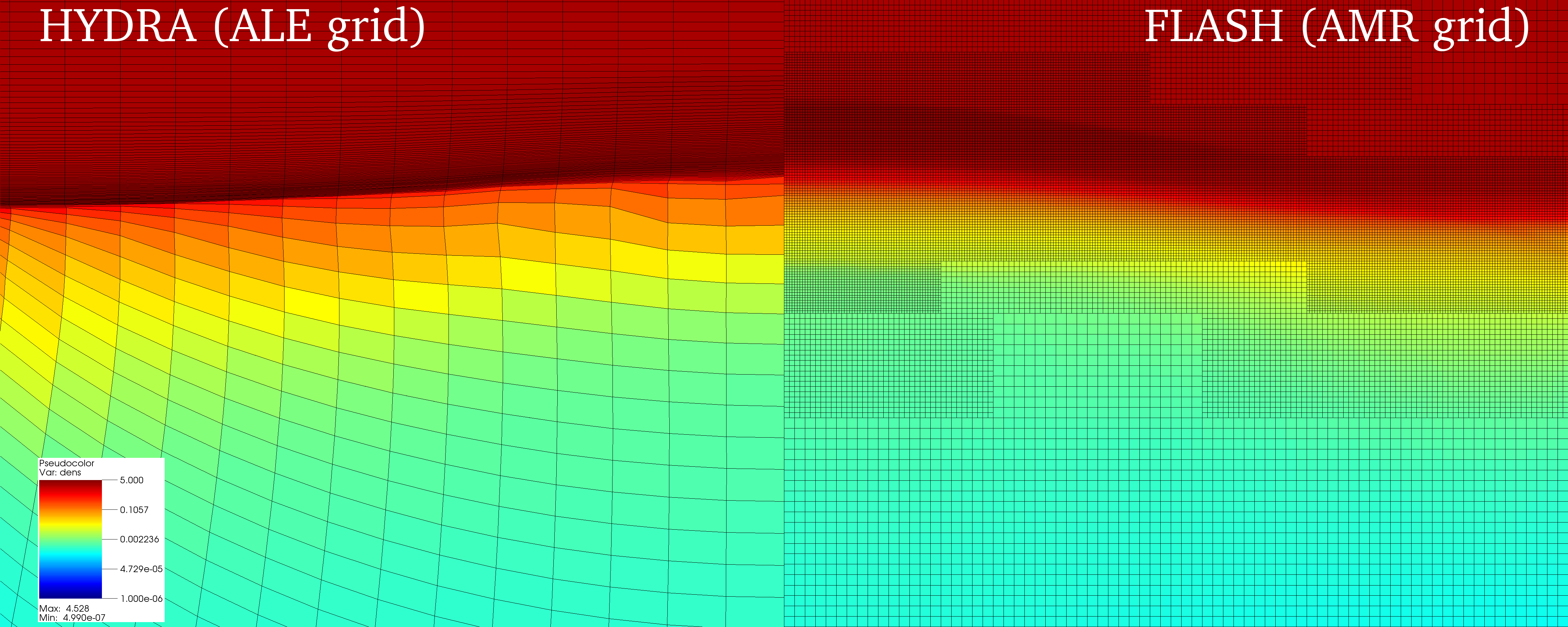
Figure 1: Snapshots of the density from a HYDRA (left) and a FLASH (right) pre-pulse simulation with the computational mesh overlayed. Results shown are for the 15.3 mJ pre-pulse at $t=1.0$ ns; density units are in g cm^-3 and total grid dimensions are 30 $\mu$m x 75 $\mu$m. Laser rays travel from the bottom to the top, irradiating target material at the top center of the plot.

III.1 ALE versus Eulerian AMR

Apart from the subtle differences in the physics implemented in HYDRA and FLASH, by design the codes have radically different approaches to defining and evolving the computational mesh and solving the equations of hydrodynamics. Whereas FLASH performs its hydrodynamic calculations on a fixed, finite volume Eulerian grid that can be refined (or de-refined) on the fly to maintain high resolution in interesting areas using AMR, by contrast the ALE approach used by HYDRA allows the grid to distort and move with the fluid flow with (preferably) minor deviations from this Lagrangian behavior to prevent severe tangling of the mesh. As an illustration of these two methods, Fig. 1 shows a density snapshot from the 15.3 mJ pre-pulse test (described in § IV) at $t=1$ ns with the grid overlayed.

Choosing one grid scheme over another also substantially changes the forms of the differential equations solved. We highlight the ramifications of choosing one scheme over another using the continuity equation; i.e.,

$$\frac{\partial\rho}{\partial t}+\nabla\cdot(\rho\vec{v})=0,$$ (7)

where $\rho$ is the mass density of the fluid and $\vec{v}$ is the vector field of the fluid velocity. An AMR grid scheme is an essentially Eulerian approach; therefore at each cell the density is represented at a fixed point in space in a fixed volume, $V_{i}$, so that the total cell mass, $m_{i}$ increases or decreases with the cell density, $\rho_{i}=m_{i}/V_{i}$, as fluid moves into or out of the cell. With this in mind the continuity equation at a cell can be rephrased as

$$\frac{\partial\rho_{i}}{\partial t}=\frac{\partial}{\partial t}\left(\frac{m_{i}}{V_{i}}\right)=\frac{1}{V_{i}}\frac{\partial m_{i}}{\partial t}=-\left[\nabla\cdot(\rho\vec{v})\right]_{i},$$ (8)

where the right hand side is the divergence of the mass flux into the cell.

This result can be compared to an ALE grid scheme, which is an essentially Lagrangian approach that instead keeps the mass in each cell, $m_{i}$, (at least approximately) fixed as the mesh expands and flows with the fluid. In examining the consequences of this approach, it is helpful to recast Eq. 7 in a more suggestively Lagrangian form,

$$\left(\frac{\partial}{\partial t}+\vec{v}\cdot\nabla\right)\rho+\rho\nabla\cdot\vec{v}=0.$$ (9)

The term in the parenthesis is readily identified as the time derivative in the frame of the moving fluid $(\equiv D/Dt)$. The continuity equation for a cell moving with the fluid flow becomes

$$\frac{D\rho_{i}}{Dt}=-\rho_{i}\left[\nabla\cdot\vec{v}\right]_{i},$$ (10)

and once again, $\rho_{i}=m_{i}/V_{i}$, so that the left hand side of this expression becomes

$$\frac{D\rho_{i}}{Dt}=\frac{D}{Dt}\left(\frac{m_{i}}{V_{i}}\right)=m_{i}\frac{D}{Dt}\left(\frac{1}{V_{i}}\right).$$ (11)

Using Eq. 11 in Eq. 10,

$$\frac{1}{V_{i}}\frac{DV_{i}}{Dt}=\left[\nabla\cdot\vec{v}\right]_{i}.$$ (12)

This result has important consequences because it means that a strong divergence of the fluid flow, as is generic in laser ablation, will expand the cells and consequently lower the resolution near the critical density where most of the laser energy is deposited. Conventionally, and, for example, in the HYDRA simulation presented in Fig. 1, users of purely-Lagrangian and ALE codes will initialize a simulation with significantly higher resolution in the solid or near-critical-density regions that will absorb most of the laser energy in order to maintain modest resolution throughout the grid after these cells have become stretched by the ablative flow.

To be absolutely precise, Eqs. 10-12 are exact for purely-Lagrangian codes but are only approximately true for ALE codes such as HYDRA. A fuller presentation would describe how ALE codes can apply a “re-zoning” operation to prevent severe tangling of the mesh, which will result in a (preferably small) change to the mass in each cell (Knupp et al., 2002; Kucharik, 2006, and references therein).

The loss of resolution in purely Lagrangian and ALE meshes does not automatically mean that the AMR approach is better suited to computationally efficient modeling of ablation-driven plasmas. For example, the literature has documented problems where the AMR scheme can yield poor results Quirk (1994); Tasker et al. (2008); Springel (2010). Suffice it to say that neither the ALE nor the AMR scheme has been definitively proven to be better-suited for modeling laser ablation. In this paper we hope to gain some insight into this question; however, as discussed in the next section, the physics in the two codes is not exactly the same. Also, any discrepancies stemming directly from the choice of grid scheme should disappear at sufficiently high resolution Robertson et al. (2010). It may be that the fine meshes shown in Fig. 1 are already in this regime. The principal difference between the two methods may simply be in making different decisions for the spatially-varying and time-varying resolution of the computational grid. (The FLASH simulations presented here, for example, determine the refinement level based on changes in mass density and electron temperature.) As in a recent astrophysical code comparison for modeling galaxy formation (Scannapieco et al. (2012) and commentary in Hopkins (2012)), we expect that the hydrodynamic behavior is well-captured by both schemes but that other assumptions – such as those discussed in the next section – are where more important differences can emerge.

III.2 EOS & Opacity Models

An obvious place where discrepancies can arise is in the different EOS models used by the two codes. Without any special reasons to prefer one EOS model for Aluminum over another, we present FLASH simulations using the SESAME model Lyon and Johnson (1992), and the commercially-available PROPACEOS model Macfarlane et al. (2006). These well-respected models can at least highlight the EOS dependence of the FLASH results relative to HYDRA, which uses either the QEOS More et al. (1988) or LEOS model. (The Al slab pre-pulse tests were performed with the LEOS model while the V-shaped groove validation experiment was modeled using QEOS.) Intuitively, it is important to note that the EOS model controls not only the pressure of the plasma, given a density and temperature, but also affects the efficiency of heat conduction by determining the mean ionization fraction, $\bar{Z}$, as well as the specific heat in Eqs. 1 & 2. Aside from subtleties in interpolation, these models can disagree on the quantities of interest by up to factors of a few in some density-temperature regimes Heltemes and Moses (2012).

Discrepancies may also arise from differences in opacity models. The FLASH results presented here use only the PROPACEOS model for the opacity of Aluminum, while the HYDRA results discussed here use an average-atom opacity model developed at LLNL. However, the opacities can only be a source of discrepancy in cases where radiation-energy loss plays an important role. Since the atomic number of Al is still relatively low, the usual channel for energy loss through Bremsstrahlung (Zel’dovich and Raizer, 1967, Ch. V.) is not necessarily a large effect. So although the opacity models from different research groups can disagree at the level of a few to tens of percent, we regard the opacity model to be of secondary importance when searching for the cause of differing results.

III.3 Treatment of the Laser

For both of the problems investigated here, the laser model in FLASH differs from HYDRA in that HYDRA includes the ponderomotive force (a.k.a. light pressure) of the laser as an extra term in the momentum equation Berger et al. (1998). However, the ponderomotive force for the most intense laser pulse we consider here ($10^{13}$ W/cm²) is smaller than atmospheric pressure and should be overwhelmed by the plasma pressure for any solid-density plasma hotter than room temperature. Therefore the lack of ponderomotive force in FLASH should be a negligible source of error at these intensities.

Both FLASH and HYDRA deposit the laser energy on the grid using the inverse bremsstrahlung approximation in the sub- to near-critical density regions where the laser rays propagate. Both codes use the Kaiser Kaiser (2000) algorithm to calculate the trajectories of the rays and interpolate the deposited energy to the computational mesh at each timestep. For the 2D cartesian geometry of the V-shaped groove problem the setup and refraction of these rays should be nearly identical in the two codes. For the 2D cylindrical Aluminum slab simulations described in the next section, there are some differences in the simulation setup. In FLASH, a few thousand laser rays, each weighted by the spatial profile of the laser spot, enter the grid parallel with each other and are not actually permitted to refract laterally in order to ensure that the laser energy is deposited as smoothly as possible. (Earlier tests in which the rays were allowed to refract laterally gave very similar results but with somewhat more noise in the energy deposition.) By contrast, the rays in HYDRA converge with an f/3 ratio and refraction away from the laser axis is allowed. Essentially, the FLASH code is set up with the aim of maximizing the smoothness of the energy deposition (as the Flash Center currently encourages its users to do) while HYDRA is set up to maximize the correspondence between simulated rays and real laser rays, as is the customary way of modeling pre-pulses at LLNL.

III.4 Remaining Minor Differences

While the HYDRA simulations discussed here include heat conduction via both electrons (Eq. 5) and ions, the FLASH simulations neglect the contribution from ions. Heat conduction is proportional to the thermal velocity of the species, therefore the contribution from ions is suppressed relative to that of electrons by a factor of $\sqrt{m_{\rm ele}/m_{\rm ion}}\sim 0.0045$ for Al. Although the next FLASH release will include this effect, we neglect it here.

Finally, as a stand-in for vacuum, the FLASH & HYDRA simulations include very low density Helium ($5\cdot 10^{-7}$ g cm^-3 unless noted otherwise) outside the target. There may be subtle differences in the way that FLASH & HYDRA treat the Al/He interface as the ablated aluminum expands into the low density He. As the ablated Al moves away from the target, some of the kinetic energy of the high-velocity Al is transferred to the He ions, which, being low density, are super-heated, creating an out-of-equilibrium (a.k.a. 3T) shock Shafranov (1957); Mihalas and Mihalas (1984); Fatenejad et al. (2011). But since the super-heated Helium is very low density the properties of the expanding Al further upstream from this interface are, in practice, insensitive to the specific value for the density of the vacuum-like He. Nevertheless, for completeness, it bears mentioning that the treatment of this shock is another place where the codes may yield different behavior.

IV Code-to-Code Comparisons for an Aluminum Slab Target Irradiated by a Laser Pre-Pulse

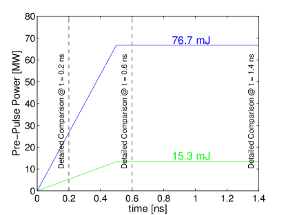
Figure 2: Total laser power versus time for the pre-pulse tests. We present detailed comparisons of the results at $t=$0.2 ns, 0.6 ns, and 1.4 ns for the 15.3 mJ pre-pulse in Fig. 4 and for the 76.7 mJ pre-pulse in Fig. 5.

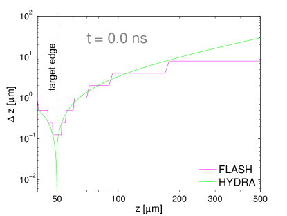
Figure 3: Comparing the initial spatial resolution through the laser axis ($r=0,z$). The Aluminum slab target edge is at 50 $\mu$m and extends leftward of this mark.

In this section, we describe code-to-code comparisons between FLASH and HYDRA for a problem in which an Al slab is irradiated by a laser pre-pulse.

IV.1 Design and Simulation Setup

We chose to compare the two codes for two different pre-pulse energies, 15.3 mJ & 76.7 mJ, using a 0.5 ns linear ramp up and 0.9 ns of constant power as in the temporal profile shown in Fig. 2. During the first few tens of femtoseconds, the laser energy deposition will heat and ionize the target, taking it from room temperature all the way to the plasma regime. The fluid approximation is at least partially invalid during these first few moments, but since ionization and heating happens quickly this (possibly inaccurate) phase only occurs for a brief interval after which the familiar ablation front and hot corona have formed, which can adequately be described by the approximations discussed earlier (§ II). Conceivably, then, the two codes may differ in these first few instants but agree well for much of the later evolution. We highlight the results at $t=0.2$ ns as a gauge of how various quantities appear early on but after this transition has taken place. The choice of highlighting $t=1.4$ ns, by contrast, is motivated to show the results after 0.9 ns of steady laser power, while the $t=0.6$ ns comparison shows the plasma properties fairly soon after the ramp-up has reached the plateau. We show results at these three times for both the 15.3 mJ and 76.7 mJ pre-pulse levels assuming a 20 $\mu$m full width at half maximum (FWHM) gaussian beam. For reference, the pre-pulse of the Titan laser (LLNL) is estimated to be 8.5 mJ deposited in 2.3 ns, with most of the energy deposition occurring in the last $\sim$1.0 ns Ma et al. (2012) while the 76.7 mJ pre-pulse is somewhat more akin to deliberate pre-pulses or intrinsic pre-pulses at large laser facilities MacPhee et al. (2010). Note that Akli & Orban et al. Akli et al. (2012) used FLASH to successfully model the pre-pulse of the Titan laser interacting with an Aluminum cone target in order to create initial conditions for Particle-in-Cell modeling of the ultra-intense pulse interaction. The FLASH simulation in Akli et al. (2012) was run in an analogous way to the FLASH simulations presented in this section, with 2D cylindrical geometry, similar laser intensities and pulse durations and the same version of the FLASH code.

Already, at $t=0$, before any evolution has been computed, the codes are set up in different ways to handle the problem. Fig. 3 compares the resolutions of the two codes through the laser axis at $r=0$. The AMR scheme in FLASH gives rise to the jagged appearance of the line showing the FLASH resolution. These simulations employ six levels of mesh refinement to span resolutions from 0.125 $\mu$m to 8 $\mu$m. In HYDRA the resolution changes smoothly except close to the edge of the target at $z=50$ $\mu$m where it becomes extremely fine, $\approx 10^{-3}\mu$m for the smallest cell. Although this might seem excessive, it is common practice to set up ALE grids in this way, anticipating that the ablation will coarsen the grid because of the many orders of magnitude change in density that will occur.

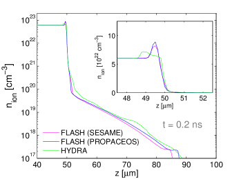
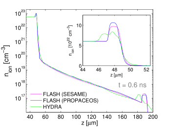
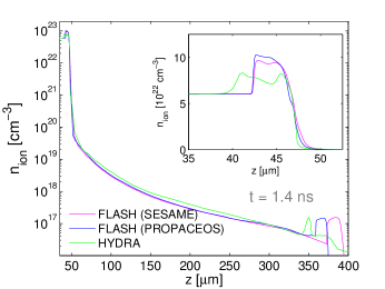
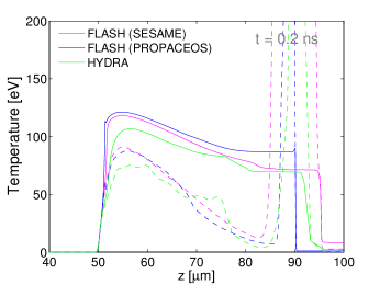
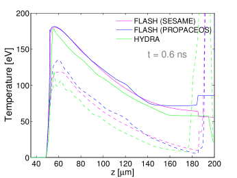
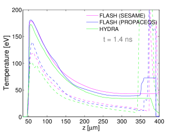
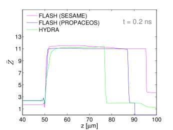
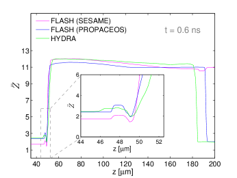
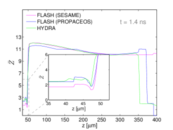
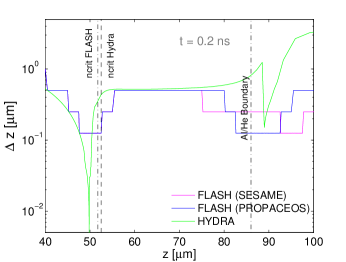
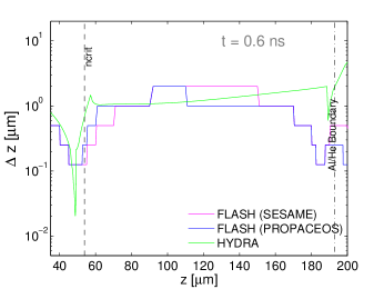
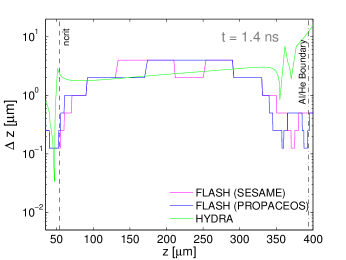
Figure 4: Results from simulations of 15.3 mJ pre-pulse irradiation of an Aluminum slab target. Panels show HYDRA results (green) and FLASH results using two different EOS models (magenta for SESAME, blue for PROPACEOS). Left-column panels are for $t=0.2$ ns, middle-column panels are $t=0.6$ ns, right-column panels are $t=1.4$ ns. The top panels show ion densities, the next-to-top row panels show electron temperatures in solid lines and ion temperatures in dashed lines, the next-to-bottom row of panels show the mean ionization state of the plasma and the bottom row of panels compare the resolutions of the computational meshes. All plots compare quantities along the laser axis ($r=0,z$).

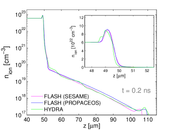
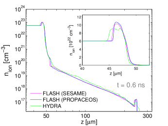
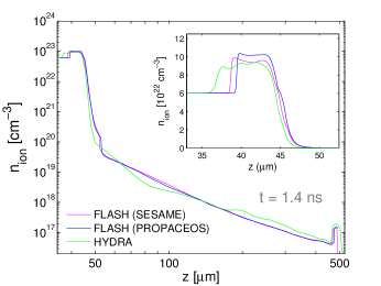
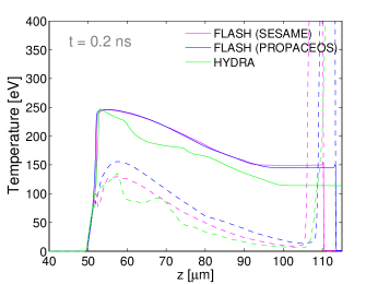
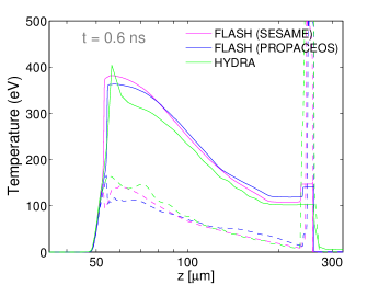
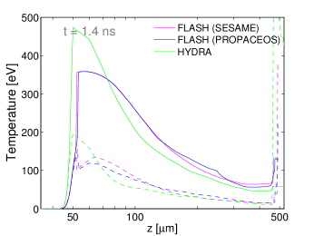
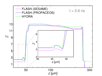
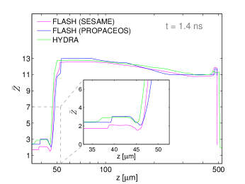
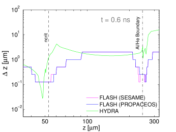
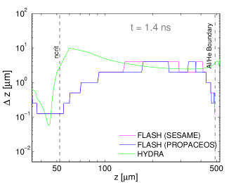
Figure 5: Results from simulations of 76.7 mJ pre-pulse irradiation of an Aluminum slab target. Panels are as described in Fig. 4.

IV.2 Results

Fig. 4 presents detailed profiles of the plasma properties through the laser axis at $t=0.2$ ns, 0.6 ns, and 1.4 ns for the 15.3 mJ pre-pulse simulations. Fig. 5 presents this same information for the 76.7 mJ pre-pulse. HYDRA results are shown with green lines while FLASH results are shown for with two different EOS models: magenta for SESAME and blue for PROPACEOS. All FLASH simulations use opacity data from PROPACEOS.

Surveying the top three panels in both figures, it is clear that the plasma expansion proceeds quite similarly in both codes and mostly independent of the choice of EOS in FLASH. For the purpose of using these pre-pulse simulations as initial conditions for PIC simulations of short-pulse laser interactions, the plasma expansion with time and change in density profile are the single most important aspects of the resulting pre-plasma properties. While Figs. 4 & 5 also show the electron and ion temperatures and mean ionization states, the ion motion due to the pre-pulse alone will be negligible over the duration of a short-pulse ultra-intense laser-matter interaction and hence the results of the PIC simulation should be insensitive to the initial ion temperature. Likewise, the field and electron-impact ionization from the ultra-intense pulse are likely to be strong enough that the sensitivity, at fixed ion density, to the mean ionization state or the initial electron temperature will also be low. This being the case, the second-highest rows, which compare electron (solid lines) and ion (dashed lines) temperatures show a great deal of similarity between the FLASH and HYDRA results. Well away from the Al/He interface at low densities, FLASH gives slightly hotter results. This may stem from increased absorption or slightly lower heat capacity. The electron temperatures in HYDRA deviate more from the FLASH results in the 76.7 mJ test. However the HYDRA resolution at the critical surface coarsens to $\Delta z\sim 10\mu$m by the end of this simulation, and so the spike in the electron temperature at the $t=1.4$ ns output is unphysical.

At very low plasma densities and around the Al/He interface, the ion temperatures skyrocket as the Al blowoff plasma shock heats the cold, low density helium initially at rest outside the Al target. The relatively long timescale of electron-ion thermal equilibrium and the comparatively rapid timescale of electron heat conduction prevent the electrons from becoming super-heated as well, as discussed in Mihalas and Mihalas (1984), and originally investigated in Shafranov (1957). This essential physics is in both codes and although there may be differences in how this shock is handled, we focus our attention on the results at higher densities since He is merely a stand-in for vacuum conditions.

Regarding the mean ionization state results in the second from the bottom columns in Figs. 4 & 5, the $\bar{Z}$ values are typically consistent to within $\pm 0.5$, except at the Al/He interface. In the under-dense corona, away from the target, the PROPACEOS and SESAME models do about equally well in matching the $\bar{Z}$ from HYDRA, while the near-or-slightly-above solid density $\bar{Z}$ results highlighted by the inset figures strongly favor the PROPACEOS model as the most HYDRA-like way of running FLASH (at least for Aluminum plasmas).

The bottom row of panels in Figs. 4 & 5 compare the spatial resolutions in FLASH and HYDRA. The most striking result is that the resolution at the critical surface in HYDRA quickly becomes an order of magnitude coarser than in FLASH. The HYDRA error bars in Fig. 6, where we highlight the motion of the critical density along the laser axis, reflect this result with the large size of the 76.7 mJ error bars especially apparent. As discussed earlier, the cell stretching in HYDRA is closely coupled to the divergence of the fluid velocity whereas in FLASH the resolution is decided by other means. Regardless, the motion of the critical density in FLASH and HYDRA is consistent to within $\lesssim 2\mu$m with neither the use of PROPACEOS nor SESAME models for the EOS standing out as agreeing better with the HYDRA result.

Overall, FLASH and HYDRA agree reasonably well for densities significantly away from where the Al/He interface occurs and in moderate-to-high resolution regions. Despite important differences between the AMR and ALE schemes for determining the computational mesh and other details discussed in Sec. III, most of the remaining differences seem attributable to the different EOS models employed in the simulations. A possible exception to this are the near-solid-density regions shown by the inset figures in the upper panels of Figs. 4 & 5. In both the 15.3 mJ and 76.7 mJ cases the above-solid-density feature in HYDRA is lower in density and further into the target at all outputs. This discrepancy is still to be adequately explained and we discuss it further in Sec. VII.

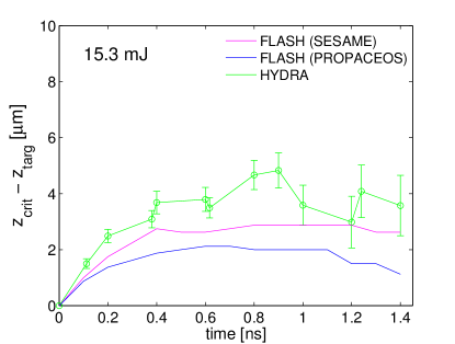
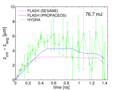
Figure 6: Position of critical density ($n_{c}=1.1\cdot 10^{21}$ cm^-3) along the laser axis versus time relative to its initial position at the target edge ($z_{\rm targ}=50\,\mu$m). Upper panel shows results for the 15.3 mJ pre-pulse while the lower panel shows results for the 76.7 mJ pre-pulse. Since the resolution at the critical density in the HYDRA results (green) is generally much coarser than in FLASH (magenta or blue, depending on the EOS model) we show the HYDRA results with error bars to indicate the cell size at critical density.

V Code-to-Code Comparisons and Validation for an Aluminum Slab Target With a V-Shaped Groove Irradiated by a Rectangular Laser Beam

This section describes code-to-code comparisons between FLASH and HYDRA for an experiment that was carried out at Colorado State University and modeled using HYDRA in which an Al target with a V-shaped groove is irradiated by a rectangular laser beam Grava et al. (2008). The data from the experiment was used as a powerful validation test for HYDRA in Grava et al. (2008). In this section the data will be used as a validation test for FLASH for the first time.

The Grava et al. Grava et al. (2008) study is unique in both the quality of the experimental data collected and in the sophistication of the radiative-hydrodynamic modeling with HYDRA, which is described in some detail. In the experiment, the V-shaped groove target is irradiated by a rectangular 360 $\mu$m FWHM laser pulse with peak intensity $\sim 10^{12}$ W/cm². The temporal behavior of this pulse, approximately 120 ps FWHM, is shown in Fig 10 of Grava et al. (2008).

The geometry of the groove-shaped target, which is reminiscent of a well-known validation experiment on the NOVA laser Wan et al. (1997); Stone et al. (2000), allows interferometric measurements of the electron density in the blowoff plasma with a few-ns cadence. Importantly Grava et al. Grava et al. (2008) use soft x-ray (46.9 nm wavelength) interferometry to conduct this measurement, which implies a critical density of $5\cdot 10^{23}$ cm^-3. Taking into account instrumental resolution and other details puts the largest measurable electron density at $5\cdot 10^{20}$ cm^-3.

Grava et al. Grava et al. (2008) pursued the experiment as a scaled version of astrophysically occurring radiative shocks, explaining that the radiative energy loss timescale in the problem, $\tau_{\rm rad}$, is comparable to hydrodynamic expansion timescale, $\tau_{\rm hydro}$. It was also significant that earlier NOVA experiments along these lines led to some puzzling results, raising the question whether collisionless Particle-In-Cell (PIC) codes might actually be more appropriate to the experimental regime than rad-hydro codes Wan et al. (1997). Grava et al. and later work by that collaboration Filevich et al. (2009); Purvis et al. (2010) showed that rad-hydro codes can indeed be trusted for these experiments, and for a variety of different elements.

Grava et al. focused on an experiment with Aluminum, the same target material as in the pre-pulse investigation in § IV. Restricting our investigation to Aluminum greatly simplifies the task of doing code-to-code comparisons and validating the HEDP extensions of FLASH. We hope to investigate other validation experiments with other target materials in the near future Filevich et al. (2009); Purvis et al. (2010).

V.1       Non-Radiative Results:
Electron Number Density

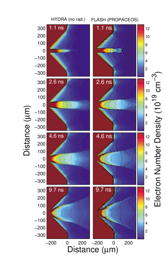
Figure 7: Electron number densities at various times from a HYDRA simulation of the irradiation of a V-shaped groove without including radiation diffusion (left panels) and results from the same setup with FLASH using the PROPACEOS equation of state, also without radiation transport (right panels). HYDRA panels are adapted with permission from Fig. 9 in Grava et al. Grava et al. (2008) (copyrighted by the American Physical Society).

Grava et al. present HYDRA results with and without multi-group radiation diffusion to demonstrate the effect of radiation on their simulation results. We use the non-radiative HYDRA simulations as a starting point for our code-to-code comparison since it removes any dependence on the opacity model. Fig. 7 shows our primary result for simulations without radiation transport. For brevity, we only show FLASH results in this section with the PROPACEOS EOS, which produced better agreement with HYDRA in the previous section and came closest to resembling the HYDRA results in Fig. 7. The simulation results in Fig. 7 show that the two codes do qualitatively agree. There are no important features in the HYDRA results that do not appear in the FLASH results and many of the contours from the simulations bear a remarkable resemblance to each other. The FLASH results in the blowoff plasma, for reasons connected to earlier discussions regarding the stretching of ALE cells, are somewhat higher resolution than the HYDRA results and therefore there may be slight differences between the results merely because FLASH is resolving the plasma in more detail. Convergence with resolution could be explored in more depth; however, the purpose of the comparison in Fig. 7 is merely to show that the FLASH simulation is realistic enough to pursue results including radiative effects. It is clear from Fig. 7 that FLASH passes this test.

V.2   Results including Radiation:
Electron Number Density

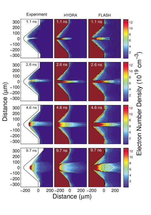
Figure 8: Comparing inferred electron number density from soft x-ray interferometry (left column) to HYDRA (center column) and FLASH (right column) simulations, both including multi-group radiation diffusion. The FLASH simulation uses PROPACEOS opacity and EOS data. Left and center columns are adapted with permission from Fig. 9 in Grava et al. Grava et al. (2008) (copyrighted by the American Physical Society).

As discussed earlier, the simulations discussed here use a diffusion approximation to model the effect of radiation Castor (2004), which provides a channel for energy to escape from the hot plasma, thus lowering the temperature and consequently the pressure. As a result, plasmas with large radiative-energy fluxes can be compressed to higher densities than non-radiating plasmas. This physics is evident in comparing the non-radiative results in Fig. 7 to the radiative results in Fig. 8, which includes the experimental measurements of electron number density in the left hand column. The ablating plasma is colliding with itself at 1.1 ns (as in Fig. 7), creating a relatively thin line of high density, high temperature Aluminum extending from the target. But instead of rebounding from the high pressure, thus creating the feature in Fig. 7 at 2.6 ns and 4.6 ns, the Aluminum stays compressed for longer so that at 4.6 ns in Fig. 8 an only slightly broadened version of this feature remains. Only between the 4.6 ns and 9.7 ns snapshots is there time enough for the pressure to broaden the feature beyond recognition. For a more extreme example of the effect of radiation in this problem see the Cu or Mo results in Purvis et al. (2010).

Despite the possibility of important differences arising from either the implementation of multi-group diffusion or in the opacity models used, the radiative results shown in Fig. 8 exhibit agreement between HYDRA and FLASH at essentially the same level as the non-radiative results shown in Fig. 7. Importantly, the agreement with the experimental data is qualitatively good as well.

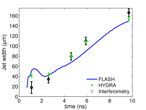
Figure 9: A quantitative comparison of the jet width versus time as inferred from the electron number density (Fig. 8) on a line perpendicular to the laser axis that is centered at (0,0). HYDRA results (green points) and interferometric measurements (black points) from Grava et al. Grava et al. (2008) are presented at 1.1, 2.6, 4.6, 5.9 and 9.7 ns. Measurements from the FLASH simulation (solid blue line) are more finely spaced in time. For brevity, the comparison at 5.9 ns is not shown in Fig. 8.

As a quantitative comparison, Fig. 9 compares the width of the jet versus time. The jet width is measured as the distance between the most steeply rising features in the electron density along a line perpendicular to the laser axis centered at (0,0). This definition is convenient for inferring the jet width from the figures in Grava et al. Grava et al. (2008) since the point of steepest rise is simply where the electron number density contours are closest together. The HYDRA results in Fig. 9 are assigned an error bar of $\pm$ 2.5 $\mu$m which is a typical distance between these two closest contours. Likewise, the jet width from the interferometric measurements is measured from the contours of electron number density in the same way. The error bars for the interferometric jet width are estimated as roughly half the distance between the fringes ($\pm 7.5\,\mu$m), except at 1.1 ns when the jet is still forming. The true resolution of the interferometric data may be slightly smaller than indicated in Fig. 9, although, in principle, a slight misalignment of the laser on target would be an additional source of uncertainty Purvis et al. (2010). In the FLASH simulations the jet width can be inferred in a precise way according to the definition above and at a number of outputs.

Fig. 9 shows that the HYDRA result is typically closer to the interferometry than the FLASH result which slightly underpredicts the jet width at 4.6 ns and 5.9 ns. The reason for this is unclear. The lower resolution of the HYDRA simulation may have enlarged the jet to some degree. Interestingly, both FLASH and HYDRA overpredict the width of the jet at 1.1 ns.

V.3 Results including Radiation:
Electron Temperature and Mean Ionization State

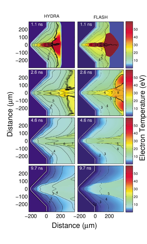
Figure 10: Comparing electron temperatures in radiation-hydrodynamics simulations from HYDRA (left column) to results from FLASH (right column); the FLASH simulation uses PROPACEOS opacity and EOS data. Contours for the mean ionization state, $\bar{Z}$, are overplotted. HYDRA panels are adapted with permission from Fig. 6 in Grava et al. Grava et al. (2008) with permission (copyrighted by the American Physical Society).

Fig. 10 compares the electron temperatures in FLASH and HYDRA at the same times reported in Fig. 8. In comparing these results, it is important to note that the interface between the Aluminum blowoff plasma and the vacuum density Helium is visible in the 1.1 ns and 2.6 ns results. The $\bar{Z}$ contours in Fig. 10 show where this boundary occurs because the plasma goes from significantly ionized Al to a region where $\bar{Z}$ can at most be equal to two. As a result there is a kind of pileup of contours moving steadily away from the target; by 4.6 ns this transition is off the grid. Rightward of this interface at 1.1 ns, Fig. 10 indicates that the FLASH simulation has somewhat higher He temperatures than the HYDRA simulation. Without giving credence to the idea that this difference is especially meaningful, it could stem from a difference in handling the non-equilibrium (i.e. $T_{\rm ele}\neq T_{\rm ion}$) nature of the shock interface or, more prosaically, the He density in FLASH may simply be lower than what was assumed but not reported in Grava et al. Grava et al. (2008). The FLASH simulation assumes the same He density, $\rho=5\cdot 10^{-7}$ g/cm³, as in the pre-pulse tests in Sec. IV.

Leftward of this Al/He interface, in the Al blowoff plasma, the results are again qualitatively similar with the FLASH results being slightly hotter than HYDRA at 1.1 ns. Some combination of this slightly higher temperature and differences in the tabulated data for the mean ionization state make the FLASH blowoff plasma slightly more ionized than the HYDRA result. The $\bar{Z}$ contours in Fig. 10 are consistent with an overall $\Delta\bar{Z}\sim 1$ difference between the two simulation results. A closer look at the FLASH output for 1.1 ns reveals that this is true for the highest ionization state as well, and we find some regions where $\bar{Z}\sim 11$. Grava et al. state that the highest mean ionization state in their simulations is $\bar{Z}\sim 10$ and that this result is confirmed by the absence of signatures of more-highly-ionized charge states in extreme UV spectroscopy. Nevertheless, both FLASH and HYDRA simulations agree that the mean ionization state never reaches $\bar{Z}\sim 12$, which would require much higher temperatures.

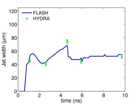
Figure 11: A quantitative comparison of jet width versus time as measured from the distance between the peaks in the mean ionization state ($\bar{Z}$) on a line perpendicular to the laser axis that is centered on (0,0). The HYDRA measurements (green points) come from the $\bar{Z}$ contours in Fig. 10, which are derived from Grava et al. Grava et al. (2008). Measurements from the FLASH simulation (solid blue line) are presented at finely spaced intervals in time.

To quantify the level of agreement in Fig. 10, the mean ionization state contours can be used as another measure of the width of the jet versus time. Material ablated from the walls will expand and collide with the plasma on axis which, up to and before 5 ns, creates a unique feature where the temperature and mean ionization state peaks just above and below the laser axis instead of on the laser axis itself. The two-finger-like appearance of the mean ionization state contours in Fig. 10 arises from this interaction. By drawing a line between the “fingers” in the contours, the distance between these peaks in the mean ionization state on the line perpendicular to the laser axis centered at (0,0) can be inferred for each output. Fig. 11 compares this measurement from the HYDRA simulations to a very precise measurement of distance between these peaks in $\bar{Z}$ from the FLASH simulation for a number of outputs. At 4.6 ns and earlier this definition of the jet width gives similar results as Fig. 9, however at around 5 ns and later the $\bar{Z}$ feature is much less pronounced because a transition is taking place in which the plasma arriving at the center is no longer plasma that was directly heated by the laser (c.f. Fig. 10 in Grava et al. Grava et al. (2008)). The speed and momenta of the impact from plasma arriving from the walls at the center has decreases significantly and a new maxima in $\bar{Z}$ forms closer to the laser axis. The abrupt transition to smaller jet width in Fig. 11 around 5 ns comes from transitioning to this new maxima.

Having explained the features and subtleties of Fig. 11, it is clear that the two codes agree well on the jet width according to the peak in the mean ionization state. This is in spite of the overall $\Delta\bar{Z}\sim 1$ difference in the mean ionization state mentioned earlier. Since there is no experimental measurement of the mean ionization state of the plasma, Fig. 11 is strictly a comparison of the two codes.

V.4 Results including Radiation: Total Pressure

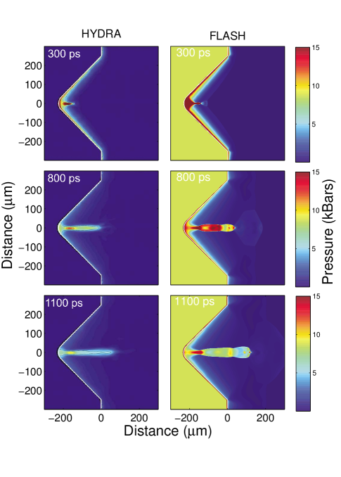
Figure 12: Comparing total plasma pressure at early times from radiation-hydrodynamics simulations from HYDRA (left column) and FLASH (right column). The FLASH simulation was performed using PROPACEOS opacity and EOS data. HYDRA panels are adapted from Fig. 8 in Grava et al. Grava et al. (2008) with permission (copyrighted by the American Physical Society).

Fig. 12 presents a comparison of the total plasma pressure at early times in the radiation-hydrodynamics simulations. While both FLASH and HYDRA use EOS data that are the same as or related to the QEOS model constructed by More et al. More et al. (1988), the implementations are clearly somewhat different. In HYDRA the total pressure at solid density (i.e. well into the target) is vanishingly small, as one would expect for a cold solid. FLASH uses the (QEOS-based) PROPACEOS equation of state which achieves vanishingly small total pressures for cold solids, in part, by allowing the electron pressures to be negative. Currently, FLASH requires positive electron and ion pressures in solving the momentum equation and in interpolating EOS data. So we set to a very small, positive value the few negative electron pressures that exist in the PROPACEOS table. The $\sim 7$ kBar (olive-colored) pressures well into the target in the FLASH results thus reflect only the ion pressure reported from PROPACEOS. Bearing in mind that, from a hydrodynamic point of view, only pressure differences matter, and that laser-heated Aluminum will quickly enter a regime where the total pressure is naturally well above zero, it is understandable why this detail seems not to have affected the agreement between the two codes, given the level of agreement that we have seen in this section and in the earlier pre-pulse tests.

Morphologically, the total pressures in the blowoff plasma are qualitatively similar in the FLASH and HYDRA simulations. Since the resolution of the FLASH simulation is very likely somewhat higher than the HYDRA simulation in this region it is reasonable that the FLASH results show more detailed features. Overall, the total pressures in FLASH are slightly higher than HYDRA, probably due to slightly higher temperatures, but, again, only the pressure differences matter to the hydrodynamics and therefore the plasma expansion is very similar.

Figure 13: Lineouts along the laser axis of the component of the velocity parallel to the laser axis at various times. The thick solid lines show measurements from the FLASH simulation of a V-shaped groove target described in § V. These thick solid lines become dotted lines at the point where the cell material is mostly very low density Helium instead of Aluminum. Thin solid lines (which become dashed lines at the Al/He transition) show the same measurements from a simulation where a flat target of the same material is irradiated with the Grava et al. laser pulse.

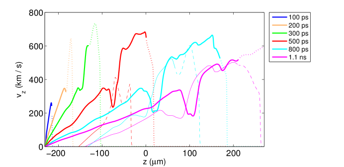
Figure 14: Lineouts along the laser axis of the component of the velocity parallel to the laser axis at various times. The thick solid lines show measurements from the FLASH simulation of a V-shaped groove target described in § V. These thick solid lines become dotted lines at the Al/He transition. Thin solid lines (which likewise become dashed lines at the Al/He transition) show the same measurements from a simulation where, similar to the target geometry of Wan et al. Wan et al. (1997), a large gap of material is missing from the center of the V-shaped groove. This target is irradiated by the Grava et al. laser pulse.

VI Formation and Properties of the Jet in the Grava et al. Experiment

The Grava et al. Grava et al. (2008) experiment had two objectives: (1) to obtain data that would make possible an important additional validation test of radiative hydrodynamics codes in the wake of the apparent failure of LASNEX Zimmerman and Kruer (1975) simulations to reproduce a similar experiment done using the Nova laser Wan et al. (1997); and (2) to create a jet analogous to astrophysics jets, following Stone et al. Stone et al. (2000). So far we have used the data from Grava et al. Grava et al. (2008) to validate the FLASH code. Here we consider the Grava et al. experiment with the second objective in mind.

Having validated FLASH for the Grava et al. experiment, we now use the FLASH simulations of the experiment to better understand the formation and properties of the jet seen in it. We focus on early times ($\leq$ 1.1 ns) and to inform our discussion we use comparisons between (1) the FLASH simulations of this experiment presented in § V, (2) FLASH simulations of a flat Aluminum target irradiated by the same rectangular laser beam used in the Grava et al. experiment, and (3) FLASH simulations of the Grava et al. experiment but with the inner $\pm 75\mu$m section of the target removed. This latter configuration resembles an earlier experiment done by Wan et al. Wan et al. (1997) in which two slabs with a gap between them were oriented perpendicular to each other and irradiated by beams of the NOVA laser. Grava et al. Grava et al. (2008) cite this experiment as an important motivation for their work.

A number of questions naturally arise in drawing parallels between the self-colliding blowoff plasma in Grava et al. and astrophysical jets. While the radiative cooling timescale may be similar in magnitude to the hydrodynamic expansion timescale (and therefore the adiabatic cooling timescale) in both problems, how similar are they in other respects? Here we address three specific questions about the formation and properties of the jets seen in the laser experiments whose answers enable us to compare them with astrophysical jets:

1. What determines the physical conditions (e.g., the density, temperature, and velocity) in the core of the jet?

2. Is the collimating effect of the the plasma ablating from the angular sides of the groove due to thermal pressure (i.e., the internal energy of the ablating plasma) or ram pressure (i.e., the component of the momentum of the ablating plasma perpendicular to the mid-plane of the experiment)?

3. Does the collimation of the flow by the plasma ablating from the angular sides of the groove and the entrainment of this plasma in the resulting jet increase or decrease the velocity of the jet?

VI.1 What determines the physical conditions in the core of the jet?

Figures 9 & 11 show that the width of the jet at early times ($\leq$ 1.1 ns) is similar to the width of the rounded region of the groove in the Al slab at the mid-plane, which is relatively flat and so relatively perpendicular to the laser beam illuminating the target. The incident laser beam has a Gaussian cross section with a full width such that most of the laser energy is deposited within $\pm 100\mu$m of the laser axis. Accordingly, the intensity of the laser beam will be much greater on the relatively flat portion of the target than on the sloping sides of the V-shaped groove. This suggests that the velocity in the core of the jet might be produced by the same physical mechanism that produces the velocity of the flow when an Al slab target is illuminated by a laser (e.g. as in § IV); namely, heating of the Al target by the laser followed by free expansion of the heated target material due to the thermal pressure of the hot electrons.

To investigate this possibility, we have compared lineouts of the velocity along the mid-plane for the two problems at five relatively early times ($\leq$ 1.1 ns). Figure 13 shows the results. Ignoring the very high ($v_{z}~{}\gtrsim~{}350$ km/s) velocities of very low density gas and focusing on $v_{z}\lesssim 350$ km/s, the velocity profiles for the two problems agree closely at all five times, supporting our conjecture that the mechanism producing them is the same. The differences seen between the two simulations at very high velocities ($v_{z}\gtrsim 350$ km/s) are at very low densities, as already mentioned, and near or approaching the transition from cells that are mostly Aluminum to cells that are mostly very low density Helium. This transition is marked by a change in line type from thick solid to dotted lines for the V-shaped target or from thin solid to dashed lines for the flat target. Because the Helium serves only as an approximation to vacuum conditions, the results at this very low density interface are both questionable and irrelevant to the questions we are concerned with in this section.

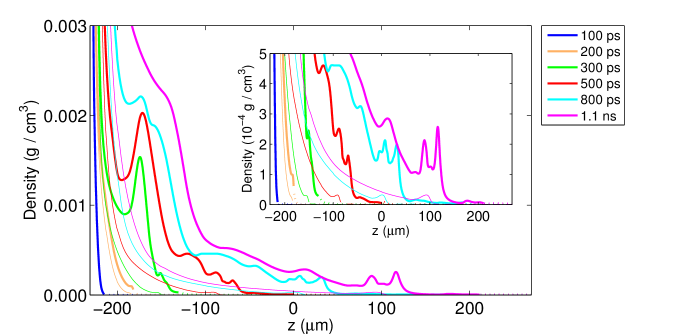
Figure 15: Lineouts of the mass density along the laser axis at various times. The thick solid lines show measurements from the FLASH simulation of a V-shaped groove target described in § V. Thin solid lines show the same measurements from a simulation where a flat target of the same material is irradiated with the Grava et al. laser pulse. As in Fig. 13, a change in line type to dotted or dashed indicates the Al/He transition.

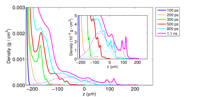
Figure 16: Lineouts of the mass density along the laser axis at various times. The thick solid lines show measurements from the FLASH simulations of a V-shaped groove target described in § V. Dashed lines show the same measurements from a simulation where, similar to the target geometry of Wan et al. Wan et al. (1997), a large gap of material is missing from the center of the V-shaped groove. This target is irradiated by the Grava et al. laser pulse. As in Fig. 14, a change in line type to dotted or dashed indicates the Al/He transition.

We have also compared these same lineouts of the velocity along the mid-plane for an Al target with a V-shaped groove, which was used in the Grava et al. Grava et al. (2008) experiment, and for a target consisting of two Al slabs oriented perpendicular to each other with a gap between them, similar to the Wan et al. Wan et al. (1997) experiment. This comparison allows us to contrast the properties of the jet produced by an Al target with a V-shaped groove that has a relatively flat portion near the mid-plane and one that does not. Figure 14 shows the results with the V-shaped groove simulation with thick solid lines of various colors depending on the output and the Wan et al.-like simulation shown likewise with thin solid lines. As in Fig. 13 a change of line type indicates the transition from mostly Aluminum to mostly Helium. Again ignoring the high velocities ($v_{z}\gtrsim 350$ km/s) that occur at low densities, the two velocity profiles differ greatly. The absence of a relatively flat portion of the target near the mid-plane means that formation of the jet is delayed until the plasma ablating from the sloping sides of the target has had time to meet at the mid-plane. Furthermore, the velocity profile of the jet is much shallower and its maximum velocity is much smaller. The results provide further support for the hypothesis that the physical mechanism producing the jet in the Grava et al. experiment is the same as in the slab problem.

Figure 15 compares lineouts of the density along the mid-plane for the V-shaped groove target used in the Grava et al. experiment (thick solid lines) and an Al slab target (thin solid lines), while Fig. 16 compares the same quantity from the V-shaped groove target (thick solid lines) and for a target consisting of two Al slabs oriented perpendicular to each other with a gap between them (thin solid lines), similar to the Wan et al. (1997) experiment. As in Figs. 13 & 14 these lines become dotted or dashed when the cells are mostly He instead of Al.

Clearly, ablation from the sloping sides of the V-shaped groove confines the flow, as discussed by Wan et al. Wan et al. (1997) and Grava et al. Grava et al. (2008), greatly increasing the density in the jet relative to the density in the case of the Al slab target, where the flow can expand laterally as well as away from the surface of the target. Collimation of the flow by the plasma ablating from the sloping sides of the V-shaped groove in the Grava et al. experiment raises the question of whether the collimation is due primarily to thermal pressure or to ram pressure. We now address this question.

VI.2 Is the collimating effect of the plasma ablating from the angular sides of the groove due to thermal pressure or ram pressure?

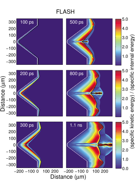
Figure 17: Plotting the ratio of $e_{\rm kin}/e_{\rm int}$ at various times for the FLASH simulation of the V-shaped groove described in § V. The original target location is shown with a white line. The transition from mostly Al to mostly He cells is indicated with a solid black line in each panel.

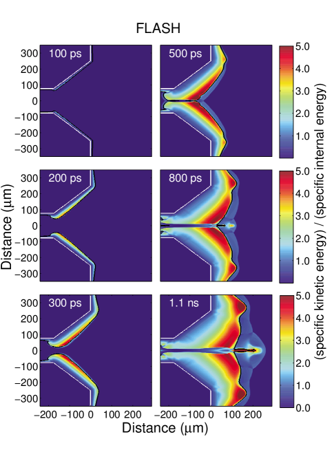
Figure 18: Plotting the ratio of $e_{\rm kin}/e_{\rm int}$ at various times for a FLASH simulation of a target with a gap in the center (similar to Wan et al. 1997) that is irradiated by the Grava et al. laser pulse. The original target location is shown with a thick white line. The transition from mostly Al to mostly He cells is indicated with a solid black line in each panel.

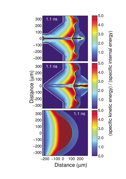
Figure 19: Plotting the ratio of $e_{\rm kin}/e_{\rm int}$ at 1.1 ns for three different FLASH simulations: (Top) the V-shaped groove simulation described in § V, (middle) results from a V-shaped groove with a gap as in Wan et al. (bottom) results from a FLASH simulation of a flat target that is likewise irradiated by the Grava et al. laser pulse. In each plot the original target location is shown with a thick white line. The transition from mostly Al to mostly He cells is indicated with a solid black line in each panel.

To address this question, we calculate the ratio of the specific kinetic energy,

$$e_{\rm kin}=\frac{1}{2}|\vec{v}|^{2}$$ (13)

to the total specific internal energy,

$$e_{\rm int}=e_{\rm ele}+e_{\rm ion}.$$ (14)

If $e_{\rm kin}/e_{\rm int}\gg 1$, the kinetic energy of the ablation flow is dominant; if instead, $e_{\rm kin}/e_{\rm int}\lesssim 1$ the internal energy due to the temperature of the plasma is dominant.

Figure 17 shows the ratio $e_{\rm kin}/e_{\rm int}$ throughout the computational domain at six different times for the Al slab target with a V-shaped groove, while Figure 18 shows the same quantity at the same times for the Al target comprised of two slabs oriented perpendicularly to each other with a gap in between, similar to the Wan et al. experiment. Figure 19 compares the same quantity for an Al slab target, and the Grava et al. and Wan et al.-like targets at 1.1 ns. In all three figures, we see a similar behavior: even at very early times, in the plasma very near the target, the internal energy of the plasma dominates the kinetic energy of the bulk flow away from the target, but further out the kinetic energy of the bulk flow dominates the internal energy. Once the laser turns off, the region where the kinetic energy of the bulk flow dominates the gas internal energy begins to grow substantially larger.

Examining the properties of the ablation flow as it approaches the mid-plane, we see that the internal energy of the plasma dominates at distances $<~{}50~{}\mu$m from the target, but the kinetic energy of the bulk flow dominates at all larger distances. This indicates that the collimation of the jet is due primarily to ram pressure except very near the target, where it is due primarily to thermal pressure of the hot plasma.

The plasma in the jet is heated when the plasma ablating from the sloping sides of the target in both the Grava et al. and the Wan et al.-like experiments collides with it and the kinetic energy in the bulk flow of the ablating plasma is released. The ratio $e_{\rm kin}/e_{\rm int}$ is small where this happens. However, the ratio is large in the mid-plane because the outward velocity in the jet is so large. The result is a complex lateral structure within the jet in which $e_{\rm kin}/e_{\rm int}$ is large in the core of the jet and small at its edges, and large again in the ablating plasma above and below the jet. This is the origin of the double-horn structure evident at very late times in the electron density, which can be seen in Figures 7-9 and in the ionization state, which can be seen in Figures 10-11.

While the complex lateral structure of the jet in these experiments is qualitatively similar to astrophysical jets, it differs in that the ratio $e_{\rm kin}/e_{\rm int}$ in astrophysical jets is expected to be large in the core of the jet and progressively smaller values further away from the jet axis with $e_{\rm kin}/e_{\rm int}\rightarrow 0$ in the ambient medium (e.g. Stone and Norman, 1993).

VI.3 Does the ablation from the angular sides of the groove increase or decrease the velocity of the jet?

We are now in a position to address whether the ablating plasma from the angular sides of the groove in the target increases or decreases the velocity of the jet. A key piece of information is that the velocity of the jet is much smaller in the Wan et al.-like experiment in which the target is two Al slabs oriented perpendicular to each other with a gap in between than in the Grava et al. experiment in which the target is an Al slab with a V-shaped groove it it. We can now understand the reason why from the answer we obtained to the previous question. The energy density of the ablating plasma is dominated by its bulk kinetic energy by the time it approaches the mid-plane, except at very small distances ($<50~{}\mu$m) from the target. The component of the momentum of the ablating plasma that is perpendicular to the mid-plane will go into heating the jet, while the component parallel to the mid-plane will add to the velocity of the jet. However, because the laser intensity is much lower away from the mid-plane, due both to the profile of the laser beam and the slanted angle of the surface of the groove, the specific internal energy (i.e., the internal energy per gram) generated by the component of the momentum of the ablating plasma when the ablating plasma collides with the jet, and the specific component of the momentum of the accreting plasma parallel to the mid-plane (i.e., the momentum per unit mass) are both smaller than in the jet flow itself, which is generated by the most intense part of the laser beam illuminating the nearly flat part of the groove near the mid-plane. This suggests that the entrainment in the jet of the plasma ablating from the sloping sides of the groove will decrease slightly the velocity of the jet compared to the velocity along the mid-plane of the freely expanding plasma in the case of a slab target. This expectation is consistent with the results shown in Figure 13.

VII Discussion of Code-to-Code Comparisons

We find excellent agreement between the FLASH and HYDRA simulations for both the pre-pulse problem described in Sec. IV and the V-shaped groove-target problem investigated in Sec. V. In this section, we consider the differences between the two codes that are described in Sec. III and comment on the remaining discrepancies or differences found in both suites of tests generally rather than focusing on any particular result.

As already noted, the two codes were not run with the same EOS and opacity data, and therefore the small discrepancies that do exist can reasonably be attributed to this fact, rather than to anything more fundamental, such as the different computational mesh schemes they use, which we described in Sec. III.1. We consider that differences in the EOS models are likely to be a larger source of uncertainty than the opacity data: comparing Figs. 7 and 8, the effect of including radiative-energy loss is still relatively subtle, and FLASH simulations of the pre-pulse tests without radiation (not shown) gave very similar results to the simulations that include radiation transport that we described in Sec. IV.

To explore the extent to which different EOS models affect the results, we presented FLASH simulations from both the PROPACEOS and SESAME EOS models for the pre-pulse problem. For the V-shaped groove targets, we presented only the PROPACEOS EOS for brevity, but we did perform FLASH simulations with the SESAME EOS. The results did not agree nearly as well with the experimental measurements of electron number density and the HYDRA simulations. This result, taken together with the finding in Figs. 4 and 5 that the PROPACEOS $\bar{Z}(\rho,T)$ model near solid density agrees much better with HYDRA than does the SESAME model, indicates that using the PROPACEOS model is the most HYDRA-like way of running FLASH and, of course, validation using the interferometry data from Grava et al (2008) implies that it is also the most accurate approach, at least for Aluminum plasmas at these densities and temperatures.

The only systematic difference between the FLASH and HYDRA results that cannot be attributed to the EOS models is the near-solid-density results in the pre-pulse problem, highlighted by the inset figures in the upper panels of Figs. 4 & 5. Regardless of the EOS, the above-solid-density features are typically somewhat more pronounced in FLASH and are not as far into the target as with HYDRA, although the resolution in this region is reasonably high for both codes.

Of all the differences between FLASH and HYDRA discussed in Sec. III, the lack of the ponderomotive force in FLASH would seem to be a likely culprit, since by $t=0.2$ ns the above-solid-density feature is already further into the target in HYDRA, and it is at very early times when the plasma pressure is low that the ponderomotive force may become a non-negligible effect. However, HYDRA pre-pulse simulations without the ponderomotive force (not shown) gave identical results for the early-time plasma properties. The lack of the ponderomotive force in FLASH is therefore unlikely to be the explanation of the discrepancy. Conceivably, as discussed in Sec. III.3, the difference could arise from the convergence of the laser rays on the target in HYDRA as opposed to the initially parallel rays in FLASH. However, Fig. 6 indicates $\lesssim 5\mu$m movement of the critical surface over the duration of the simulation, and the discrepancy appears at early times (even before $t=0.2$ ns), so this hypothesis seems unlikely, and the differences remain unexplained.

Unfortunately, the simulations of the Al target with a V-shaped groove, which involve electron densities below the $\sim 5\cdot 10^{20}$ cm^-3 experimental threshold of detection, add little to the discussion. Despite this lingering issue, the properties of the Aluminum blowoff plasma are in reasonably good agreement between the codes and with the experimental data. Since PIC simulations of short-pulse laser interactions with pre-formed plasmas depend crucially on the plasma properties near or below the critical density ($n_{c}\sim 10^{21}$ cm^-3), this level of agreement is sufficient to use the output from either FLASH or HYDRA radiation-hydrodynamics simulations as initial conditions for these codes. Equivalently, the predictive accuracy of the pre-plasma properties seems to be limited only by the quality of the EOS and opacity data, and the accuracy of the measurements of the pre-pulse properties.

VIII Conclusions

We carried out a series of studies comparing the FLASH code to previously-published and new simulations from the HYDRA code used extensively at LLNL. These tests include a comparison of results at pre-pulse intensities and energies (15.3 mJ and 76.7 mJ) for an Aluminum slab target in 2D cylindrical geometry over 1.4 ns of evolution. We also compared the results of FLASH to previously-published experimental results and HYDRA modeling for the irradiation of a mm-long V-shaped groove cut into an Aluminum target as a test of the code in a 2D cartesian geometry Grava et al. (2008). Importantly, these experiments, conducted at Colorado State University, included soft x-ray interferometric measurements of the electron density in the Al blowoff plasma as a powerful validation test.

In all cases the FLASH results bore a remarkable resemblance to results from HYDRA. This is especially true for the properties of the underdense Al blowoff plasma, which matters most for the use of these codes in calculating pre-plasma properties as initial conditions for PIC simulations of ultra-intense, short-pulse laser-matter interactions.

These code comparisons were performed without using the same EOS and opacity models. To assess the extent to which differences in EOS models can change the results, we presented simulations with FLASH using both the PROPACEOS and SESAME EOS models. While these simulations gave similar results, the PROPACEOS model gave the most HYDRA-like way of running the code and also agreed better with the interferometric measurements of the electron number density in the V-shaped groove experiment.

One difference between the FLASH and HYDRA results could not be attributed to differences in EOS: the above-solid-density ablation front moving into the target in the pre-pulse tests typically peaked at slightly higher density in FLASH, and typically had moved slightly further into the target in HYDRA. We were able to rule out the lack of ponderomotive force (a.k.a. light pressure) in FLASH as the explanation for this by looking closely at HYDRA pre-pulse simulations with and without the ponderomotive force which yielded identical results. This confirmed our intuition that the ponderomotive force is negligible for pre-pulse intensities and energies, and therefore the FLASH treatment of the laser as a source of energy deposition only should be an exceedingly good approximation in the pre-pulse regime.

Having validated the FLASH simulations for the Al target with a V-shaped groove, we have also used these FLASH simulations to better understand the formation and properties of the jet in the experiment. We show that the velocity of the jet is produced primarily by the heating of the target in the relatively flat region of the V-shaped groove at the mid-plane, as in standard slab targets. We show that the jet is collimated primarily by the ram pressure of the plasma that ablates from the sloping sides of the groove. We find that the interaction of the plasma ablating from the sloping sides of the groove with the jet produces the observed complex lateral structure in it, a structure that is qualitatively similar to astrophysical jets but differs significantly from them, quantitatively. Finally, we show that the entrainment in the jet of the plasma ablating from the sloping sides of the groove slightly decreases the velocity in the jet compared to the velocity along the mid-plane of the freely expanding plasma in the case of a slab target.

For the FLASH code, which has historically been used primarily for astrophysics, this full-physics code comparison and validation of a number of new HEDP-relevant algorithms, and investigation into the physics of the laboratory-produced jet represents a milestone in the realization of FLASH as a well-tested open-source tool for radiation-hydrodynamics modeling of laser-produced plasmas. More testing can and should be done. We focused on laser-irradiated Aluminum plasmas. High-quality interferometric data also exists for C, Cu and Mo Filevich et al. (2009); Purvis et al. (2010). Any future FLASH investigations using these materials would do well to start with these validation tests.

References

- Akli et al. (2012) K. U. Akli, C. Orban, D. Schumacher, M. Storm, M. Fatenejad, D. Lamb, and R. R. Freeman, Phys. Rev. E 86, 065402 (2012).
- Boehly et al. (1997) T. R. Boehly, D. L. Brown, R. S. Craxton, R. L. Keck, J. P. Knauer, J. H. Kelly, T. J. Kessler, S. A. Kumpan, S. J. Loucks, S. A. Letzring, et al., Optics Communications 133, 495 (1997).
- Moses et al. (2009) E. I. Moses, R. N. Boyd, B. A. Remington, C. J. Keane, and R. Al-Ayat, Physics of Plasmas 16, 041006 (2009).
- Lindl et al. (2011) J. D. Lindl, L. J. Atherton, P. A. Amednt, S. Batha, P. Bell, R. L. Berger, R. Betti, D. L. Bleuel, T. R. Boehly, D. K. Bradley, et al., Nuclear Fusion 51, 094024 (2011).
- Rosen et al. (2011) M. D. Rosen, H. A. Scott, D. E. Hinkel, E. A. Williams, D. A. Callahan, R. P. J. Town, L. Divol, P. A. Michel, W. L. Kruer, L. J. Suter, et al., High Energy Density Physics 7, 180 (2011).
- Lamb and Marinak (2012) D. Lamb and M. Marinak, Panel Report on Integrated Modeling, Workshop on Science of Fusion Ignition on NIF, LLNL-TR-570412 (2012), URL https://lasers.llnl.gov/workshops/science_of_ignition/.
- Bellei et al. (2013) C. Bellei, P. A. Amendt, S. C. Wilks, M. G. Haines, D. T. Casey, C. K. Li, R. Petrasso, and D. R. Welch, Physics of Plasmas 20, 012701 (2013).
- Thomas and Kares (2012) V. A. Thomas and R. J. Kares, Phys. Rev. Lett. 109, 075004 (2012), URL http://link.aps.org/doi/10.1103/PhysRevLett.109.075004.
- Marinak et al. (1996) M. M. Marinak, R. E. Tipton, O. L. Landen, T. J. Murphy, P. Amendt, S. W. Haan, S. P. Hatchett, C. J. Keane, R. McEachern, and R. Wallace, Physics of Plasmas 3, 2070 (1996).
- Marinak et al. (1998) M. M. Marinak, S. W. Haan, T. R. Dittrich, R. E. Tipton, and G. B. Zimmerman, Physics of Plasmas 5, 1125 (1998).
- Marinak et al. (2001) M. M. Marinak, G. D. Kerbel, N. A. Gentile, O. Jones, D. Munro, S. Pollaine, T. R. Dittrich, and S. W. Haan, Physics of Plasmas 8, 2275 (2001).
- Callahan et al. (2012) D. A. Callahan, N. B. Meezan, S. H. Glenzer, A. J. MacKinnon, L. R. Benedetti, D. K. Bradley, J. R. Celeste, P. M. Celliers, S. N. Dixit, T. Döppner, et al., Physics of Plasmas 19, 056305 (2012).
- Harding et al. (2009) E. C. Harding, J. F. Hansen, O. A. Hurricane, R. P. Drake, H. F. Robey, C. C. Kuranz, B. A. Remington, M. J. Bono, M. J. Grosskopf, and R. S. Gillespie, Phys. Rev. Lett. 103, 045005 (2009).
- van der Holst et al. (2012) B. van der Holst, G. Tóth, I. Sokolov, L. Daldorff, K. Powell, and R. Drake, High Energy Density Physics 8, 161 (2012), ISSN 1574-1818.
- Taccetti et al. (2012) J. M. Taccetti, P. A. Keiter, N. Lanier, K. Mussack, K. Belle, and G. R. Magelssen, Review of Scientific Instruments 83, 023506 (2012).
- DOE (2011) DOE, Basic Research Directions for User Science at the National Ignition Facility (2011).
- MacNeice et al. (2000) P. MacNeice, K. M. Olson, C. Mobarry, R. de Fainchtein, and C. Packer, Computer Physics Communications 126, 330 (2000).
- Fatenejad et al. (2013) M. Fatenejad, A. R. Bell, A. Benuzzi-Mounaix, R. Crowston, R. P. Drake, N. Flocke, G. Gregori, M. Koenig, C. Krauland, D. Lamb, et al., High Energy Density Physics 9, 172 (2013).
- Scopatz et al. (2013) A. Scopatz, M. Fatenejad, N. Flocke, G. Gregori, M. Koenig, D. Q. Lamb, D. Lee, J. Meinecke, A. Ravasio, P. Tzeferacos, et al., High Energy Density Physics 9, 75 (2013).
- Hirt et al. (1974) C. W. Hirt, A. A. Amsden, and J. L. Cook, Journal of Computational Physics 14, 227 (1974).
- Castor (2004) J. I. Castor, Radiation Hydrodynamics (2004).
- Kucharik (2006) M. Kucharik, Ph. D. Thesis, Czech Technical University in Prague 27, 1273 (2006).
- Grava et al. (2008) J. Grava, M. A. Purvis, J. Filevich, M. C. Marconi, J. J. Rocca, J. Dunn, S. J. Moon, and V. N. Shlyaptsev, Phys. Rev. E 78, 016403 (2008).
- Wan et al. (1997) A. S. Wan, T. W. Barbee, R. Cauble, P. Celliers, L. B. Da Silva, J. C. Moreno, P. W. Rambo, G. F. Stone, J. E. Trebes, and F. Weber, Phys. Rev. E 55, 6293 (1997), URL http://link.aps.org/doi/10.1103/PhysRevE.55.6293.
- Stone et al. (2000) J. M. Stone, N. Turner, K. Estabrook, B. Remington, D. Farley, S. G. Glendinning, and S. Glenzer, ApJS 127, 497 (2000).
- Spitzer (1963) L. Spitzer, American Journal of Physics 31, 890 (1963).
- Lee and More (1984) Y. T. Lee and R. M. More, Physics of Fluids 27, 1273 (1984).
- Marinak et al. (2009) M. M. Marinak, G. D. Kerbel, J. M. Koning, M. V. Patel, S. M. Sepke, P. N. Brown, B. Chang, R. Procassini, and D. Larson, in APS Meeting Abstracts (2009), p. 8100P.
- Mihalas and Mihalas (1984) D. Mihalas and B. W. Mihalas, Foundations of radiation hydrodynamics (1984).
- The Flash Center for Computational Science (2012) The Flash Center for Computational Science, User Guide Version-4.0-beta (2012).
- Atzeni and Meyer-Ter-Vehn (2004) S. Atzeni and J. Meyer-Ter-Vehn, The Physics of Inertial Fusion: Beam Plasma Interaction, Hydrodynamics, Hot Dense Matter, International Series of Monographs on Physics (Oxford University Press, 2004), ISBN 9780198562641.
- Knupp et al. (2002) P. Knupp, L. G. Margolin, and M. Shashkov, Journal of Computational Physics 176, 93 (2002).
- Quirk (1994) J. J. Quirk, International Journal for Numerical Methods in Fluids 18, 555 (1994).
- Tasker et al. (2008) E. J. Tasker, R. Brunino, N. L. Mitchell, D. Michielsen, S. Hopton, F. R. Pearce, G. L. Bryan, and T. Theuns, MNRAS 390, 1267 (2008), eprint 0808.1844.
- Springel (2010) V. Springel, MNRAS 401, 791 (2010), eprint 0901.4107.
- Robertson et al. (2010) B. E. Robertson, A. V. Kravtsov, N. Y. Gnedin, T. Abel, and D. H. Rudd, MNRAS 401, 2463 (2010), eprint 0909.0513.
- Scannapieco et al. (2012) C. Scannapieco, M. Wadepuhl, O. H. Parry, J. F. Navarro, A. Jenkins, V. Springel, R. Teyssier, E. Carlson, H. M. P. Couchman, R. A. Crain, et al., MNRAS 423, 1726 (2012), eprint 1112.0315.
- Hopkins (2012) P. F. Hopkins, ArXiv e-prints (2012), eprint 1206.5006.
- Lyon and Johnson (1992) S. P. Lyon and J. D. Johnson, SESAME: The Los Alamos National Laboratory Equation of State Database (Los Alamos National Laboratory Report, LA-UR 92-3407, 1992).
- Macfarlane et al. (2006) J. J. Macfarlane, I. E. Golovkin, and P. R. Woodruff, JSQRT 99, 381 (2006).
- Heltemes and Moses (2012) T. A. Heltemes and G. A. Moses, Computer Physics Communications 183, 2629 (2012).
- More et al. (1988) R. M. More, K. H. Warren, D. A. Young, and G. B. Zimmerman, Physics of Fluids 31, 3059 (1988).
- Zel’dovich and Raizer (1967) Y. B. Zel’dovich and Y. P. Raizer, Physics of shock waves and high-temperature hydrodynamic phenomena (1967).
- Seaton et al. (1994) M. J. Seaton, Y. Yan, D. Mihalas, and A. K. Pradhan, MNRAS 266, 805 (1994).
- Mendoza et al. (2007) C. Mendoza, M. J. Seaton, P. Buerger, A. Bellorín, M. Meléndez, J. González, L. S. Rodríguez, F. Delahaye, E. Palacios, A. K. Pradhan, et al., MNRAS 378, 1031 (2007), eprint 0704.1583.
- Berger et al. (1998) R. L. Berger, C. H. Still, E. A. Williams, and A. B. Langdon, Physics of Plasmas 5, 4337 (1998).
- Kaiser (2000) T. B. Kaiser, Phys. Rev. E 61, 895 (2000), URL http://link.aps.org/doi/10.1103/PhysRevE.61.895.
- Shafranov (1957) V. D. Shafranov, Sov. Phys. JETP 5, 1183 (1957).
- Fatenejad et al. (2011) M. Fatenejad, C. Fryer, B. Fryxell, D. Lamb, E. Myra, and J. Wohlbier, in APS Meeting Abstracts (2011), p. 8004.
- Ma et al. (2012) T. Ma, H. Sawada, P. K. Patel, C. D. Chen, L. Divol, D. P. Higginson, A. J. Kemp, M. H. Key, D. J. Larson, S. Le Pape, et al., Phys. Rev. Lett. 108, 115004 (2012).
- MacPhee et al. (2010) A. G. MacPhee, L. Divol, A. J. Kemp, K. U. Akli, F. N. Beg, C. D. Chen, H. Chen, D. S. Hey, R. J. Fedosejevs, R. R. Freeman, et al., Phys. Rev. Lett. 104, 055002 (2010).
- Filevich et al. (2009) J. Filevich, M. Purvis, J. Grava, D. P. Ryan, J. Dunn, S. J. Moon, V. N. Shlyaptsev, and J. J. Rocca, High Energy Density Physics 5, 276 (2009).
- Purvis et al. (2010) M. A. Purvis, J. Grava, J. Filevich, D. P. Ryan, S. J. Moon, J. Dunn, V. N. Shlyaptsev, and J. J. Rocca, Phys. Rev. E 81, 036408 (2010).
- Zimmerman and Kruer (1975) G. B. Zimmerman and W. L. Kruer, Comments Plasma Phys. Controlled Fusion 2, 51 (1975).
- Stone and Norman (1993) J. M. Stone and M. L. Norman, ApJ 413, 198 (1993).