Theory of Fluctuating Charge Ordering in the Pseudogap Phase of the Cuprates Via A Preformed Pair Approach

Abstract

We study the static and dynamic behavior of charge ordering within a $d$-wave pair pseudogap (pg) scenario. This is addressed using a density-density correlation function derived from the standard pg self energy, $\Sigma$ and compatible with the longitudinal and transverse sum rules. The broadening factor $\gamma$ in $\Sigma$ reflects the breaking of pairs into constituent fermions. We apply this form for $\Sigma$ (derived elsewhere for high fields) to demonstrate the existence of quantum oscillations in a non-Fermi liquid pg state. Our conclusion is that the pseudogap-induced pairbreaking, via $\gamma$, allows the underlying fermiology to be revealed; in YBCO, finite $\omega$ and $\gamma$ enable antinodal fluctuations, despite the competition with a $d$-wave gap in the static and superconducting limits.

Introduction One of the most exciting developments in the field of high temperature superconductivity has arisen recently with the growing evidence for charge ordered states Saw ; Achkar et al. (2013); Wise et al. (2008); LaForge et al. (2010); Haug et al. (2009) now evident for a range of hole concentrations in the underdoped regime. Some of the earliest indications for this charge ordering were associated with reconstructed Fermi surfaces inferred from quantum oscillations Doiron-Leyraud et al. (2007). While static charge ordering signatures appear most clearly at these high magnetic fields LeBoeuf et al. (2013), there is evidence that even in zero field there is a fluctuating or dynamic propensity Wu et al. (2011); Saw for the same charge ordering. Central to these observations is the uncertainty over the charge ordering wave-vector, which may differ in different cuprate families. There are claims that it is associated with both nodal nesting (NN) as well as anti-nodal (AN) nesting Riggs et al. (2011); Doiron-Leyraud et al. (2007); Harrison and Sebastian (2011). (Here the nomenclature reflects the nodal/antinodal anisotropy inherent in a $d$-wave order parameter.) It could be argued that a discovery of this new form of order in the cuprates presents evidence against a preformed pair interpretation of the pseudogap. Also problematic for a preformed pair scenario is the growing evidence Wise et al. (2008); Harrison and Sebastian (2011) that the charge ordering is antinodal, since the same $\mathbf{k}$ states participate in both the $d$-wave pseudogap and the AN ordering.

In this paper, because of its importance, we look more deeply into charge ordering within a scenario in which the pseudogap derives from $d$-wave preformed pairs. We do so by calculating the associated density-density correlation functions, $P_{\rho,\rho}(\mathbf{q},\omega)$ and demonstrate how dynamic charge ordering fluctuations are a reflection of the underlying fermiology in the presence of a gap. Importantly, our work begins with the widely accepted Mal ; Norman et al. (1998) form of zero field self energy which is known to give rise to Fermi arcs (with bandstructure $\xi_{\mathbf{p}}$)

$$\Sigma(P)=-i\gamma^{\prime}-\Delta_{pg}^{2}G_{0}^{\gamma}(-P)\equiv-i\gamma^{\prime}+\frac{\Delta_{pg}^{2}}{i\epsilon+\xi_{\mathbf{p}}+i\gamma}.$$ (1)

A key contribution of this paper is that we establish the form of the density-density correlation function associated with this self energy, in a manner analytically consistent with the longitudinal and transverse sum rules. Using this we investigate the zero field, $H=0$, possible instabilities (dynamic and static) in the presence of a $d$-wave pseudogap. Depending on the fermiology we find both nodal and anti-nodal dynamic charge ordering tendencies. Our work emphasizes the latter. Coexistence of (albeit, dynamic) anti-nodal charge ordering and the pseudogap is shown to derive from the “pairbreaking” contribution (associated with $\gamma$ in Eq. (1)) to the density-density correlation function. This pair breaking dominates the quasi-particle scattering (or nesting) contribution to the spectral weight at low $T$. Stated alternatively, pairs need to be broken into their composite fermions in order to contribute to the charge correlation function. Finite frequency enables this pairbreaking. Since $\gamma$ is necessarily absent in the superconducting self energy where the condensate pairs are infinitely long lived, we conclude that the pseudogap (with $\gamma\neq 0$) plays an important role in enabling antinodal charge fluctuations.

We secondarily address the implications of this self energy (Eq. (1)) for quantum oscillation experiments. We show that oscillatory behavior is found in thermodynamics for this non-Fermi liquid pseudogap phase, due primarily to the pairbreaking associated with $\gamma$. In this paper we include this study because of its relevance to charge ordering and to counter the belief that such oscillations imply Fermi liquid behavior. It should be stressed, however, that this paper is otherwise devoted to $H=0$ behavior. In earlier work we have shown Scherpelz et al. (2013) using Gor’kov theory that the same self energy applies to the very high field limit.

Our approach can be compared with others in the literature Senthil and Lee (2009); Ran where it is claimed that quantum oscillations are a signature of a high field Fermi liquid state, and argue for a three peaked spectral function Micklitz and Norman (2009).

Theory We next show how the self energy in Eq. (1) leads to a form for the diamagnetic current $\frac{\tensor{n}}{m}$ which can be used to make an ansatz for the current-current correlation function; from this one can readily infer the density-density correlation function in the pseudogap phase. From the definition of $\frac{\tensor{n}}{m}$ and by integration by parts, we can write the diamagnetic contribution in terms of the full Green’s function $G(P)$ as

$$\frac{\tensor{n}}{m} = 2\sum_{K}\frac{\tensor{1}}{m}G(K)=2\sum_{K}\frac{\partial^{2}\xi_{\mathbf{k}}}{\partial\mathbf{k}\partial\mathbf{k}}G(K)$$ (2)

$$= 2\sum_{K}G^{2}(K)\frac{\partial\xi_{\mathbf{k}}}{\partial\mathbf{k}}\frac{\partial\xi_{\mathbf{k}}}{\partial\mathbf{k}}\big{(}1-\Delta_{pg}^{2}(G_{0}^{\gamma})^{2}(-K)\big{)}.$$

Here $K=(i\omega_{n},\mathbf{k})$ and $\sum_{K}=T\sum_{n}\sum_{\mathbf{k}}$.

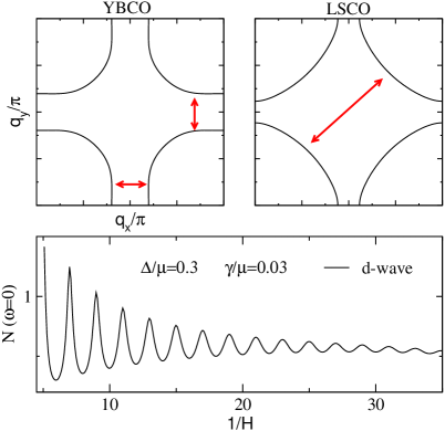
Figure 1: Fermi surfaces for YBCO and LSCO with arrows indicating the dominant nesting vectors. The lower panel shows quantum oscillations persist in a non-Fermi liquid pseudogap state, due to the finite pair lifetime reflected in $\gamma^{-1}$. Their amplitude is reduced by a factor of about 5 from the standard Lifshitz-Kosevich theory.

Now we use the constraint that there is no Meissner effect in the normal state to first determine the current-current correlation function at four-vector $Q=0$, $P_{JJ}(0)$, and then reconstruct $P_{JJ}(Q)$. This latter ansatz however will be tested against two sum rules. Using Eq. (2) a reasonable inference is

$${\tensor{P}_{JJ}}(Q) = 2\sum_{K}\frac{\partial\xi_{\textbf{k}+\textbf{q}/2}}{\partial\textbf{k}}\frac{\partial\xi_{\textbf{k}+\textbf{q}/2}}{\partial\textbf{k}}\Big{[}G_{K}G_{K+Q}$$ (3)

$$- \Delta_{pg}^{2}G_{0,-K-Q}^{\gamma}G_{0,-K}^{\gamma}G_{K+Q}G_{K}\Big{]}.$$

This expression can be written in a more suggestive notation as

$$2\displaystyle{\sum_{K}}\frac{\partial\xi_{\textbf{k}+\textbf{q}/2}}{\partial\bf k}\frac{\partial\xi_{\textbf{k}+\textbf{q}/2}}{\partial\bf k}\Bigg{(}G_{K}G_{K+Q}-F_{pg,K}F_{pg,K+Q}\Bigg{)}$$ (4)

with $F_{pg,K}\equiv\Delta_{pg,\textbf{k}}G^{\gamma}_{0,-K}G_{K}$. Interestingly, we have found a similar result for the local density of states in an STM-based experiment Wulin et al. (2009), but with a different sign in front of the ${pg}$ contribution.

Thus far, we have discussed the current-current correlation function. The density-density correlation function should necessarily have the same electromagnetic-vertex function structure which leads to a generalized particle-hole susceptibility

$$P_{\rho\rho}(\omega,\mathbf{q})=\sum_{\mathbf{k}}\int\frac{d\epsilon_{1}d\epsilon_{2}}{2\pi^{2}}\frac{f(\epsilon_{2})-f(\epsilon_{1})}{\omega-(\epsilon_{1}-\epsilon_{2})+i\delta}$$

$$\times \Big{[}A_{G}(\mathbf{k}+\mathbf{q},\epsilon_{1})A_{G}(\mathbf{k},\epsilon_{2})+A_{F}(\mathbf{k}+\mathbf{q},\epsilon_{1})A_{F}(\mathbf{k},\epsilon_{2})\Big{]}.$$

Here $A_{G}$ and $A_{F}$ are the spectral functions for $G$ and $F_{pg}$. This expression for $P_{\rho,\rho}$ can only be generalized below $T_{c}$ by including the important contribution from collective modes, often omitted in the literature Marra et al. (2013). Above $T_{c}$, it is complete.

The sum rules on the longitudinal (L) and transverse (T) components of the current-current correlation function are a central constraint on our ansatz. These are given by:

$$\int^{+\infty}_{-\infty}\frac{d\omega}{\pi}\big{(}-\frac{\textrm{Im}P_{JJ}^{L}(\omega,\mathbf{q})}{\omega}\big{)} = \frac{n}{m}$$

$$\textrm{and}\leavevmode\nobreak\ \leavevmode\nobreak\ \leavevmode\nobreak\ \lim_{q\rightarrow 0}\int_{-\infty}^{+\infty}\frac{d\omega}{\pi}\big{(}-\frac{\textrm{Im}P_{JJ}^{T}(\omega,\mathbf{q})}{\omega}\big{)} = \frac{n}{m}.$$ (5)

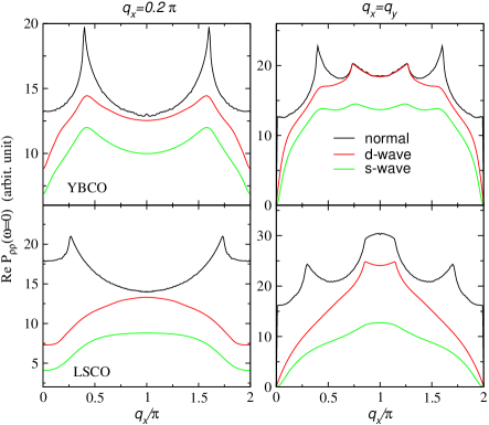
Figure 2: Static studies: Vertical and diagonal cuts plotting Re$P_{\rho,\rho}(\omega=0)$ vs $\mathbf{q}$ for YBCO and LSCO. The black, red and green lines are for normal gas, $d$-wave and $s$-wave pseudogaps, respectively. The $d$-wave gap is compatible with nodal peaks but suppresses anti-nodal peaks. Here $\gamma\approx 0$.

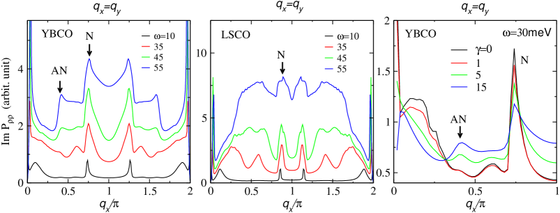
Figure 3: Dynamical studies: Left and Central Figures show diagonal cuts of Im$P_{\rho,\rho}$ vs $\mathbf{q}$ for $d$-wave with YBCO and LSCO bandstructure, and $\gamma\approx 0$. The peaks located at $q_{x}=q_{y}\approx 0.75\pi$ and $q_{x}=q_{y}\approx 0.4\pi$ become visible between $10-\leavevmode\nobreak\ 35\leavevmode\nobreak\$meV, and correspond to the nodal (N) and anti-nodal (AN) peaks we observed in Re$P_{\rho,\rho}$ of the (gapless) normal gas. There is also a small peak which appears at $q_{x}=q_{y}\approx 0.6\pi$ in the $d$-wave curves for $\omega\approx\Delta$. The plot on the right shows the effect (for YBCO) of varying $\gamma$ at fixed frequency where one sees that larger $\gamma$ enhances the anti-nodal $q_{x}\approx 0.4\pi$ peak while decreasing the relative height of the nodal $q_{x}\approx 0.75\pi$ peak.

Importantly, these sum rules can be analytically proved using Eq. (1) and Eq. (3). The second of these is the weaker condition, as it provides no real check on the finite $Q$ behavior of the correlation functions. Indeed, above $T_{c}$ it can be thought of as an equivalent condition to the requirement that there is no Meissner effect. The longitudinal sum rule represents a more stringent test and is equivalent to proving a current conservation condition.

To see this Not , note that the electromagnetic vertex function can be extracted from the ansatz in Eq. (3). This vertex satisfies $\Gamma^{\mu}(K+Q,K)-\gamma^{\mu}(K+Q,K)$

$$=\Delta_{pg}^{2}\gamma^{\mu}(-K-Q,-K)G^{\gamma}_{0}(-K-Q)G^{\gamma}_{0}(-K)$$ (6)

which is consistent Not with the Ward Identity $q_{\mu}\Gamma^{\mu}(K+Q,K)=G^{-1}(K+Q)-G^{-1}(K)$. With this full vertex and Ward identity, one can verify that the correlation functions satisfy the current conservation condition $q^{\mu}Q^{\mu\nu}=0$, so that, for example

$$\Omega{\bf Q}_{\rho J}-\mathbf{q}\cdot\tensor{Q}_{JJ}=0.$$ (7)

Here $\tensor{Q}_{JJ}\equiv\tensor{P}+\frac{\tensor{n}}{m}$, and ${\bf Q}_{\rho J}\equiv 2\sum_{K}\frac{\partial\xi_{\mathbf{k}+\mathbf{q}/2}}{\partial\mathbf{k}}G(K+Q)G(K)$. Using Eq. (7), with $\Omega=0$, we find $\frac{\mathbf{q}\cdot\tensor{Q}_{JJ}(0,\mathbf{q})\cdot\mathbf{q}}{q^{2}}=P^{L}_{JJ}(0,\mathbf{q})+\frac{n}{m}=0$. It then follows that $P^{L}_{JJ}(0,\mathbf{q})=\int^{+\infty}_{-\infty}\frac{d\omega}{\pi}\frac{\textrm{Im}P^{L}_{JJ}(\omega,\mathbf{q})}{\omega}=-\frac{n}{m}$. which proves consistency between Eq. (3) and the longitudinal sum rule.

Quantum Oscillations To address the theory of quantum oscillations, we make use of the fact that specific heat data Riggs et al. (2011) suggest that even in the high magnetic fields the pseudogap persists. Moreover, we have earlier shown Scherpelz et al. (2013) from Gor’kov theory that at high fields, when there is only intra-Landau level pairing Dukan et al. (1991), a BCS-like dispersion persists. Notably, the gap or pseudogap parameter is inhomogeneous, but for some purposes Stephen (1992), this inhomogeneity can be averaged over in a vortex liquid or a pseudogap phase. A major effect of non-zero field is to replace the dispersion $\xi_{\mathbf{p}}$ by the appropriate Landau level quantization. With this replacement, one can compute an extension of the usual Lifshitz-Kosevich (LK) formula (based on Eq. (1)) to arrive at an analytic formula for the density of states as a function of magnetic field. The density of states at the Fermi energy is then given by $N(0)=\frac{H}{(2\pi)^{2}}\sum_{n,k_{z}}\frac{\gamma}{\pi(E_{n,k_{z}}^{2}+\gamma^{2})}$ with $E_{n,k_{z}}=\sqrt{\xi_{n,k_{z}}^{2}+\Delta^{2}}$ and $\xi_{n,k_{z}}=(n+\frac{1}{2})\omega_{c}+\frac{k_{z}^{2}}{2m}-\mu$, with $\omega_{c}=eH/m$. Using the Poisson sumation formula, one finds a simple (for the $s$-wave case) analytic expression for the oscillatory contribution which depends on non-zero $\gamma$. A similar analysis follows for the $d$-wave case, although the result is less compact.

Numerical Results Henceforward, in order not to have too many distinct parameters we take $\gamma^{\prime}=\gamma$, although our qualitative findings are robust for general $\gamma^{\prime}$. To begin with, in addressing numerics one can gain analytical intuition by first considering the limit in which $\gamma=0$

$$P_{\rho,\rho}(\textbf{q},\omega)=\sum_{\mathbf{k}}\Bigg{[}\Big{(}1-\frac{\xi^{+}\xi^{-}+\Delta_{pg}^{2}}{E^{+}E^{-}}\Big{)}$$

$$\qquad\times\frac{(E^{+}+E^{-})(1-f_{+}-f_{-})}{\omega^{2}-(E^{+}+E^{-})^{2}}$$

$$-\Big{(}1+\frac{\xi^{+}\xi^{-}+\Delta_{pg}^{2}}{E^{+}E^{-}}\Big{)}\frac{(E^{+}-E^{-})(f_{+}-f_{-})}{\omega^{2}-(E^{+}-E^{-})^{2}}\Bigg{]}.$$ (8)

Here $E_{\pm}=E_{\mathbf{k}\pm\mathbf{q}/2}$, $\xi_{\pm}=\xi_{\mathbf{k}\pm\mathbf{q}/2}$ and $f_{\pm}=f(E_{\pm})$.

Importantly, this density response consists of a scattering term in the third line and (in the second line) a pair breaking or pair forming term involving $1-2f$. At the lowest temperatures, the pair breaking term dominates the spectral weight. Thus the particle-hole response of a low $T$ system with a pseudogap is only possible when pairs are broken.

In Figures 2 and 3, we plot the real and imaginary parts of the susceptibility $P_{\rho,\rho}(\omega,\mathbf{q})$ with the band structure $\xi_{k}=t_{0}+t_{1}(\cos k_{x}+\cos k_{y})/2+t_{2}\cos k_{x}\cos k_{y}+t_{3}(\cos 2k_{x}+\cos 2k_{y})/2$. Since cuprate bandstructures are somewhat variable Si et al. (1993) we consider two different parameter sets. For YBCO we take: $t_{0}=160\mbox{meV},\leavevmode\nobreak\ \leavevmode\nobreak\ \leavevmode\nobreak\ t_{1}=-600\mbox{meV},\leavevmode\nobreak\ \leavevmode\nobreak\ \leavevmode\nobreak\ t_{2}=200\mbox{meV},\leavevmode\nobreak\ \leavevmode\nobreak\ \leavevmode\nobreak\ t_{3}=-80\mbox{meV}$. For LSCO we take $t_{0}=130\mbox{meV},\leavevmode\nobreak\ \leavevmode\nobreak\ \leavevmode\nobreak\ t_{1}=-600\mbox{meV},\leavevmode\nobreak\ \leavevmode\nobreak\ \leavevmode\nobreak\ t_{2}=160\mbox{meV},\leavevmode\nobreak\ \leavevmode\nobreak\ \leavevmode\nobreak\ t_{3}=0\mbox{meV}$. This yields a square shaped Fermi surface for YBCO and a rounded shape Fermi surface for LSCO. We assume the $d$-wave pairing gap is $\Delta_{k}=\Delta_{0}(\cos k_{x}-\cos k_{y})/2$, with $\Delta_{0}=35$meV, for definiteness.

In Figure 1, we plot (from left to right) the Fermi surfaces of a normal state YBCO and normal state LSCO system. It should be clear that the preferred nesting is more antinodal in YBCO, while more nodal in LSCO. The lower figure shows quantum oscillations in YBCO via a plot of the density of states at the Fermi energy as a function of frequency in the pseudogap phase. Important here is the fact that non-zero $\gamma$ (representing the dynamic equilibrium between pairs and fermions) enables these oscillations in the presence of a pseudogap.

Figure 2 presents a study of the real part of the density-density correlation function in the static limit. The maxima in this function are generally associated with a static, i.e., true, instability of the charge disordered phase. These plots represent varying $\mathbf{q}$ along the vertical (left column) as well as diagonal (right column) directions in Re$P_{\rho,\rho}(\mathbf{q},\omega=0)$. The upper panel corresponds to YBCO and the lower to LSCO. Going from top to bottom (black, red and green) indicates the behavior for the gapless normal phase, and for the $d$- and $s$-wave paired states. The peaks for the gapless normal phase in the left panels represent the antinodal nestings and they are more apparent for YBCO. The peaks in the gapless normal phase on the right include nodal nesting and this tends to dominate in LSCO. An important observation is that static $d$-wave (or $s$-wave) pairing is highly destructive to the antinodal peak, whereas the nodal peak (particularly in YBCO) is very little affected by the $d$-wave pairing gap. In some respects this seems rather straightforward, and such competition between pairing and charge ordering in the same regime of $\mathbf{k}$ space has been discussed much earlier Levin et al. (1974). Nevertheless, this underlines the strong competition between a $d$-wave pseudogap and static antinodal charge ordering.

In Figure 3, plots are presented for the behavior of the dynamic charge susceptibility in the presence of a $d$-wave pseudogap, for diagonal cuts and a range of frequencies. The figure on the left represents YBCO (with $\gamma\approx 0$), in the center, LSCO, while the figure on the right shows the effect of variable $\gamma$ in the YBCO case. In YBCO, the antinodal (AN) peak appears somewhere between $\omega=10\leavevmode\nobreak\$meV, and $\omega=35\leavevmode\nobreak\ \mbox{meV}=\Delta_{0}$, becoming more apparent as frequency increases. (The broad feature below the nodal maximum (N) in LSCO is not a true anti-nodal peak.) At intermediate $\omega$, over a narrow range, a new peak appears, midway between, and reflecting a mixture of the nodal and anti-nodal peaks.

Important to the physical picture are the plots in the right-most panel showing $\textrm{Im}\leavevmode\nobreak\ P_{\rho,\rho}$ vs. $\mathbf{q}$ at $\omega=30\leavevmode\nobreak\$meV with varying $\gamma$. The figure demonstrates that as $\gamma$ increases the anti-nodal peak becomes relatively more important. Physically, bigger $\gamma$ can be interpreted as reflecting shorter lived pairs. That is, the size of $\gamma$ reflects the ease with which the finite-lived pairs break up into their separate fermionic components. We see in this figure that increasing $\omega$ also assists in breaking pairs, thus enabling coexistence of dynamic anti-nodal charge ordering with a $d$-wave pseudogap.

Conclusions The starting point for this paper is Eq. (1) which was derived from a microscopic t-matrix scheme Mal independent of later ARPES phenomenological arguments Norman et al. (1998). Using Gor’kov theory, we find Scherpelz et al. (2013) Eq. (1) is valid in the presence of a pseudogap in a very high magnetic field (albeit with $\gamma$ and $\Delta_{pg}$ dependent on $H$). Our microscopic model Mal was based on a particular form for the t-matrix (naturally associated with Gor’kov theory, which involves one bare and one dressed Green’s function). Importantly because of a gap in the fermionic spectrum, this form leads to long lived pairs and a two-peaked spectral function, thereby distinguishing it from other (3-peaked) models in the literature Micklitz and Norman (2009); Senthil and Lee (2009); Ran . A crucial finding here is that $H\neq 0$ quantum oscillations persist in a non-Fermi liquid phase.

We conclude quite generally that the pseudogap-phase-derived pairbreaking through the parameter $\gamma$, enables the underlying LDA-based fermiology to be revealed. Importantly, at finite $\omega$, coexistence of anti-nodal fluctuating order and a $d$-wave pseudogap becomes possible. That is, the nesting vectors seen in Figure 1 are evident in the pseudogap state with non-zero $\omega$ and $\gamma$. This underlying fermiology was seen in Fermi arcs Chien et al. (2009) and we have found it here for charge fluctuations and quantum oscillations. For the former we have shown that static nodal order coexists more readily with $d$-wave pairing, while anti-nodal ordering is more problematic. We speculate that finite, large $H$ plays a similar role as $\omega$ and $\gamma$ in enabling, through the breaking of metastable pairs, the coexistence of (in this case) a static antinodal charge ordering and a $d$-wave pseudogap, as observed LeBoeuf et al. (2013).

Work supported by NSF-MRSEC Grant 0820054. P.S. acknowledges support from the Hertz Foundation.

References

- (1) G. Ghiringhelli et al, Science 337, 821 (2012).
- Achkar et al. (2013) A. J. Achkar, F. He, R. Sutarto, J. Geck, H. Zhang, Y.-J. Kim, and D. G. Hawthorn, Phys. Rev. Lett. 110, 017001 (2013).
- Wise et al. (2008) W. D. Wise, M. C. Boyer, K. Chatterjee, T. Kondo, T. Takeuchi, H. Ikuta, Y. Wang, and E. W. Hudson, Nature Physics 4, 696 (2008).
- LaForge et al. (2010) A. D. LaForge, A. A. Schafgans, S. V. Dordevic, W. J. Padilla, K. X. Burch, Z.-Q. Li, K. Segawa, S. Komiya, Y. Ando, J. M. Tranquada, et al., Phys. Rev. B 81, 064510 (2010).
- Haug et al. (2009) D. Haug, V. Hinkov, A. Suchaneck, D. S. Inosov, N. B. Christensen, C. Niedermayer, P. Bourges, Y. sidis, P. J. T, I. A, et al., Phys. Rev. Lett. 103, 017001 (2009).
- Doiron-Leyraud et al. (2007) N. Doiron-Leyraud, C. Proust, D. leBoeuf, J. Levallois, J.-P. Bonnemaison, R. Liang, D. A. Bonn, W. N. Hardy, and L. Taillefer, Nature 447, 565 (2007).
- LeBoeuf et al. (2013) D. LeBoeuf, S. Kramer, W. N. Hardy, R. Liang, D. A. Bonn, and C. Proust, Nature Physics 9, 79 (2013).
- Wu et al. (2011) T. Wu, H. Mayaffre, M. Horvatic, C. Berthier, W. N. Hardy, R. Liang, D. A. Bonn, and M.-H. Julien, Nature 477, 191 (2011).
- Riggs et al. (2011) S. C. Riggs, V. O, J. B. Kemper, J. B. Betts, A. Migliori, F. F. Balakirev, W. N. Hardy, R. Liang, D. A. Bonn, and G. S. Boebinger, Nature Physics 7, 332 (2011).
- Harrison and Sebastian (2011) N. Harrison and S. E. Sebastian, Phys. Rev. Lett. 106, 226402 (2011).
- (11) B. Jankó, J. Maly, and K. Levin, Phys. Rev. B 56, R11407, (1997); J. Maly, B. Jankó, and K. Levin, Physica C 321, 113 (1999) and cond-mat/9710187.
- Norman et al. (1998) M. R. Norman, M. Randeria, H. Ding, and J. C. Campuzano, Phys. Rev. B 57, 11093(R) (1998).
- Scherpelz et al. (2013) P. Scherpelz, D. Wulin, K. Levin, and A. K. Rajagopal, Phys. Rev. A 87, 063602 (2013).
- Senthil and Lee (2009) T. Senthil and P. A. Lee, Phys. Rev. B 79, 245116 (2009).
- (15) S. Banerjee, Shizhong Zhang and M. Randeria: ArXiV 1210.2466.
- Micklitz and Norman (2009) T. Micklitz and M. R. Norman, Phys. Rev. B 80, 220513 (2009).
- Wulin et al. (2009) D. Wulin, Y. He, C.-C. Chien, D. K. Morr, and K. Levin, Phys. Rev. B 80, 134504 (2009).
- Marra et al. (2013) P. Marra, S. Sykora, K. Wohlfeld, and J. van den Brink, Phys. Rev. Lett. 110, 117005 (2013).
- (19) One may wonder why this self energy model so readily satisfies the 2 sum rules. This arises because the calculations parallel those for the spin response in conventional BCS theory. A sign flip in correlation functions occurs in the gap squared term involving the pseudogap, in order to avoid a Meissner effect. This leads to (a somewhat accidental) similarity with a spin response. We note there is a problem with the compressibility sum rule for the pseudogap. A more microscopic scheme arriving at the response functions discussed here first appeared in Chen et al, Phys. Rev. B 61, 11662(2000).
- Dukan et al. (1991) S. Dukan, A. V. Andreev, and A. Tesanovic, Physica C 183, 355 (1991).
- Stephen (1992) M. J. Stephen, Phys. Rev. B 45, 5841 (1992).
- Si et al. (1993) Q. Si, Y. Zha, K. Levin, and J. P. Lu, Phys. Rev. B 47, 9055 (1993).
- Levin et al. (1974) K. Levin, S. L. Cunningham, and D. L. Mills, Phys. Rev. B 10, 3821 (1974).
- Chien et al. (2009) C.-C. Chien, Y. He, and K. Levin, Phys. Rev. B 79, 214527 (2009).