LyMAS: Predicting Large-Scale Ly Forest Statistics from the Dark Matter Density Field
Abstract
We describe LyMAS (Ly Mass Association Scheme), a method of predicting
clustering statistics in the Ly forest on large scales from moderate
resolution simulations of the dark matter distribution, with calibration from
high-resolution hydrodynamic simulations of smaller volumes. We use the
“Horizon MareNostrum” simulation, a comoving volume evolved with the
adaptive mesh hydrodynamic code RAMSES, to compute the conditional probability
distribution of the transmitted flux , smoothed
(1-dimensionally) over the spectral resolution scale, on the dark matter
density contrast , smoothed (3-dimensionally) over a similar scale. In
this study we adopt the spectral resolution of the SDSS-III Baryon Oscillation
Spectroscopic Survey (BOSS) at , and we find optimal results for a dark
matter smoothing length (comoving). In its simplest form,
LyMAS draws randomly from the hydro-calibrated to convert
dark matter skewers into Ly forest pseudo-spectra, which are then used to
compute cross-sightline flux statistics. In extended form, LyMAS exactly
reproduces both the 1-dimensional power spectrum and 1-point flux distribution
of the hydro simulation spectra. Applied to the MareNostrum dark matter field,
LyMAS accurately predicts the 2-point conditional flux distribution and flux
correlation function of the full hydro simulation for transverse
sightline separations as small as , including redshift-space distortion
effects. It is substantially more accurate than a deterministic density-flux
mapping (“Fluctuating Gunn-Peterson Approximation”), often used for
large volume simulations of the forest. With the MareNostrum calibration, we
apply LyMAS to N-body simulations of a and
cube to produce large, publicly available catalogs of
mock BOSS spectra111
The LyMAS website can be found at:
http://www2.iap.fr/users/peirani/lymas/lymas.htm
![[Uncaptioned image]](/html/1306.1533/assets/x1.png) that probe a large comoving volume. LyMAS will be a powerful tool for interpreting
3-d Ly forest data, thereby transforming measurements from BOSS and other
massive quasar absorption surveys into constraints on dark energy, dark matter,
space geometry, and IGM physics.
that probe a large comoving volume. LyMAS will be a powerful tool for interpreting
3-d Ly forest data, thereby transforming measurements from BOSS and other
massive quasar absorption surveys into constraints on dark energy, dark matter,
space geometry, and IGM physics.
Subject headings:
large-scale structure of universe – quasars: absorption lines – intergalactic medium – methods: n-body simulations1. Introduction
The Ly forest – fluctuating absorption produced by intergalactic neutral hydrogen atoms in the spectra of background quasars – is the most powerful probe of cosmic structure at redshifts . The physics of Ly forest absorption is relatively well understood, thanks to numerical simulations (e.g., Cen et al. 1994; Zhang, Anninos & Norman 1995; Hernquist et al. 1996; Miralda-Escudé et al. 1996 and related analytic methods (e.g., Bi & Davidsen 1997; Hui, Gnedin, & Zhang 1997) that accurately predict its statistical properties with minimal assumptions beyond those of the standard cosmological model. The power spectrum, correlation function, and probability distribution function (PDF) of Ly forest flux have been used to constrain the underlying matter power spectrum and the thermal state of the intergalactic medium (IGM), with corresponding constraints on cosmological parameters and dark matter properties (e.g., Croft et al. 1998, 1999, 2002; McDonald et al. 2000, 2005; Zaldarriaga, Hui, & Tegmark 2001; Viel, Haehnelt, & Springel 2004; Seljak et al. 2005). These analyses have treated each sightline in isolation, as a collection of individual 1-dimensional tracks through the intergalactic gas distribution. The Baryon Oscillation Spectroscopic Survey (BOSS) of SDSS-III (Eisenstein et al., 2011; Dawson et al., 2013) is opening a new “3-dimensional” frontier in Ly forest cosmology by measuring absorption on a grid of sightlines (150,000 quasars over 10,000 square degrees) that is large enough and dense enough to enable accurate measurements of transverse correlations across sightlines separated by tens of 222Throughout the paper, we quote comoving distances in , where .. BOSS and potential successor surveys (e.g., BigBOSS, Schlegel et al. 2011) present a new theoretical challenge. For instance, the recent first measurements of Baryon Acoustic Oscillations (BAO) in the Ly forest fluctuations in the BOSS Data Release 9 (Busca et al., 2012; Slosar et al., 2013) have opened new perspectives in constraining cosmological models, but the analysis and interpretation of such data require the development of efficient theoretical tools. In particular, to accurately predict the statistics of the Ly forest at large scales for specified cosmological parameters, one must model physics on the pressure-support scale (a.k.a. the “Jeans scale”) of the IGM — about for typical values and roughly at overdensity of 10 (comoving at , see Peeples et al. 2010) — while simulating volumes many hundreds of on a side. This paper proposes and tests a new method of meeting this challenge.
Most Ly forest absorption arises in diffuse, highly photoionized gas, which is heated by photoionization and cooled adiabatically by expansion of the universe, leading to a tight correlation between temperature and density (Katz, Weinberg, & Hernquist, 1996; Hui & Gnedin, 1997). This correlation enables the Fluctuating Gunn-Peterson Approximation (FGPA; Weinberg, Katz, & Hernquist 1998; Croft et al. 1998), where the Ly optical depth is tied to the local dark matter overdensity assuming photoionization equilibrium and the Gunn & Peterson (1965) formula for neutral hydrogen absorption. The FGPA can be applied to a log-normal density field created from Gaussian initial conditions (Gnedin & Hui, 1996; Bi & Davidsen, 1997) or to the dark matter density field of an N-body simulation, with pressure effects incorporated by smoothing the field at the gas Jeans scale or by using an approximate technique (Gnedin & Hui, 1998) to incorporate pressure into the N-body evolution. Most efforts to systematically model large scale Ly forest measurements and their dependence on cosmological parameters have used some variant of this approach, with full hydrodynamic simulations used to calibrate and test it (e.g., Croft et al. 1998, 1999, 2002; Zaldarriaga, Hui, & Tegmark 2001; McDonald et al. 2005). Growing computer power enables more ambitious approaches, and Viel, Haehnelt, & Springel (2006, 2010) used grids of hydrodynamic simulations to model Ly forest statistics, but even these simulations ( on a side) are tiny compared to the volume probed by BOSS.
There are several reasons that the N-body or log-normal approaches are unsatisfactory as a tool for modeling the 3-d Ly forest. First, even without hydrodynamics, it is not currently feasible to model Gpc3 volumes while retaining good resolution on the gas Jeans scale. For example, even the heroic 30003-particle simulations analyzed by Slosar et al. (2009) have an initial particle spacing of , while smoothed particle hydrodynamic (SPH) simulations require initial separations of to yield fully converged results (Lidz et al., 2010; Peeples et al., 2010). Second, the choice of smoothing scale for the dark matter inevitably produces some ambiguity in the predictions (Zaldarriaga, Hui, & Tegmark, 2001); Ly forest statistics are insensitive to this choice, but not perfectly so (Viel et al., 2002; Peeples et al., 2010). Third, the FGPA assumes a deterministic relation between dark matter overdensity and continuum-normalized Ly flux (, hereafter simply “flux”), of the form , where is the index of the gas temperature-density relation and is a normalization constant that depends on several physical parameters (see Croft et al. 1998; Weinberg, Katz, & Hernquist 1998; Peeples et al. 2010). In practice, there is scatter around this relation because of peculiar velocities, shock heating of the gas above the temperature-density relation, and pressure-induced differences between the gas and dark matter distributions. Peculiar velocities, the largest source of scatter (Croft et al., 1997; Weinberg et al., 1999; Viel et al., 2002), can be incorporated into dark matter-based approaches, but the latter two effects require a hydrodynamic treatment. Finally, even if the FGPA were a perfect approximation on some scale (e.g., the gas Jeans scale), smoothing does not commute with the non-linear transformation between density and flux, so one cannot simply apply it to a lower resolution dark matter simulation and recover a lower resolution version of the transmitted Ly flux.
We expect that the FGPA and log-normal methods, and even linear perturbation theory with effective bias factors calibrated on hydrodynamic simulations (McDonald, 2003) are adequate on sufficiently large scales, e.g., for predicting the baryon acoustic oscillation (BAO) feature at (White, 2003; McDonald & Eisenstein, 2007; Slosar et al., 2009; White et al., 2010; Le Goff et al., 2011; Greig, Bolton & Wyithe, 2011), which is the primary target of BOSS. Font-Ribera, McDonald & Miralda-Escudé (2012) have developed an efficient semi-analytic method for generating mock data sets for the large-scale Ly forest, tailored to reproduce the observed power spectrum and PDF, which allows tests for systematics in analysis methods and calculation of statistical errors and covariance matrices. But BOSS and other 3-d Ly forest surveys will also enable precise measurements of flux correlations at scales of a few to a few tens of , where these approximations may not be accurate relative to the measurement precision. Large simulation volumes are still needed in this regime, both to eliminate systematic effects of the finite box size and to ensure that statistics are limited by the available data not by the available simulation volume. Deriving constraints and error bars requires making predictions as a function of cosmological and IGM parameters. Angulo & White (2010) have proposed an elegant and accurate method for remapping non-linear dark matter distributions from one cosmology to another, so these parameter explorations can be kept inexpensive if one can carry them out with moderate resolution N-body simulations.
In this paper, we make explicit the separation-of-scale philosophy that is already implicit in these alternative methods to predict large-scale Ly forest statistics. We concentrate on the conditional flux probability distribution (PDF), the probability of finding flux in a spectral pixel at location 2 given that the flux has the value in a pixel with transverse (projected) separation (see Miralda-Escudé et al. 1997). Other two-point statistics such as the flux correlation function can be computed by integrating over this distribution and the unconditional PDF (see §3). It seems reasonable in principle that to predict this distribution on large scales we should only need to resolve the matter distribution on scales . High-resolution hydrodynamic simulations are needed to compute the relation between the flux , smoothed (1-dimensionally) on the scale of instrumental resolution or some deliberately chosen larger scale, and the matter density contrast , smoothed (3-dimensionally) on a scale larger than the simulation resolution but smaller than the separations being probed. For the reasons discussed above, this relation is not deterministic but stochastic, described by a conditional probability distribution .
Our conjecture is that one can predict for a given cosmological and IGM model by using a moderate resolution N-body simulation to compute and convolving this with the local conditional distribution computed from high-resolution hydro simulations, evaluated for and . Physically, we are assuming that the fluxes at positions 1 and 2 are correlated because the matter densities at these positions are correlated, and that the deviation from the conditional mean is uncorrelated with the deviation . The assumption of uncorrelated deviations will certainly fail for closely neighboring pixels, whose fluxes will lie above or below the conditional mean for the same reason, but we expect it to become accurate quickly at larger separations.
We test this conjecture explicitly using a large, adaptive mesh refinement (AMR) simulation of a comoving volume, realized with dark matter particles and a top-level hydro grid, evolved with the AMR hydro code RAMSES (Teyssier, 2002). We use this simulation to calibrate the relation for several choices of dark matter and Ly smoothing scales. We then compare the Ly forest statistics computed from the gas distribution of the simulation to those computed from the dark matter distribution by the procedure described above, which we refer to as LyMAS for Ly Mass Association Scheme333French readers may appreciate the resonance with MoLUSC (Sousbie, Courtois, Bryan, & Devriendt, 2008), which utilizes a similar style of dual-level calculation to predict large scale galaxy clustering.. We also compare results to the deterministic FGPA approach applied on the same smoothing scales, finding that LyMAS is significantly more accurate at small separations. For compactness, we will sometimes abbreviate Ly forest to LyaF in the remainder of the paper.
In the next section we describe the hydro simulation and our methods for creating LyaF spectra and for extracting skewers of the smoothed dark matter density field. Section 3 presents LyMAS in its simplest form, which is designed to predict flux statistics across sightlines but does not produce realistic artificial spectra, because it ignores correlated deviations of along an individual line of sight. In §4 we describe an extended scheme that produces artificial spectra with a 1-d flux power spectrum and 1-point PDF that (almost) exactly match those of the full spectra from the hydro simulation while retaining the accurate performance of LyMAS for cross-sightline statistics. In §5 we describe the application of LyMAS to N-body simulations of a and comoving volume, illustrating the impact of finite box size on flux correlation statistics. We summarize our results and look towards future applications in §6. Finally, in the website dedicated to LyMAS, we describe several sets of electronic tables being made available with this paper, presenting the conditional flux PDFs computed from the MareNostrum hydro simulation and the mock spectra extracted from the large N-body simulations.
2. Hydrodynamic simulation and creation of spectra
In this section, we introduce the “Horizon-MareNostrum” simulation, a high resolution cosmological N-body and hydrodynamics simulation we have analyzed to generate our calibrations. We will then describe our procedures to extract from this simulation the LyaF spectra as well as DM density fields.
2.1. The “Horizon-MareNostrum” simulation
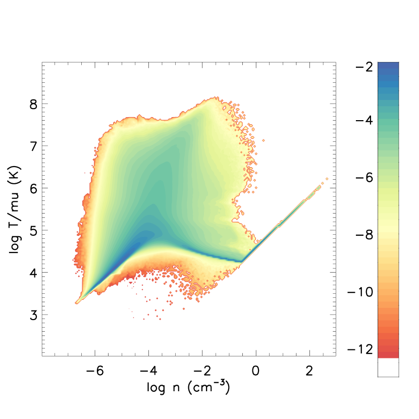
The Horizon-MareNostrum simulation (which we hereafter refer to simply as MareNostrum) was run for a CDM universe using WMAP1 parameters (Spergel et al., 2003), namely , , , km/s/Mpc, and . The simulation was performed in a periodic box of side Mpc with dark matter particles (e.g. with mass resolution of ) and an adaptive mesh refinement (AMR) technique (Teyssier, 2002) was used to keep the spatial resolution fixed at kpc in physical units. The evolution of the thermodynamic properties of the gas depends on a wide range of physical processes. In particular, MareNostrum incorporates metal-dependent cooling and photoionization heating from a UV background computed via the prescriptions of Haardt & Madau (1996), starting at a reionization redshift . A model of supernova feedback and metal enrichment has also been incorporated using the implementation described by Dubois & Teyssier (2008). The high-redshift Ly forest arises mainly in gas with overdensity , whose thermal evolution is governed primarily by photoionization heating and adiabatic cooling from the expansion of the universe. For reference, Figure 1 shows the evolution of the mean temperature of the IGM at the mean density (from to ), and Figure 2 shows the mass-weighted temperature-density diagram of the MareNostrum simulation at our analysis redshift . At densities one sees the usual sharp locus of photoionized gas, with a small fraction of gas shock heated above this relation. At higher densities one sees shock-heated gas in halos and the locus of radiatively cooled and star-forming gas in galaxies. For further details of the MN simulation, we refer the readers to previous papers that have used it for other analyses (Ocvirk et al., 2008; Devriendt et al., 2010).

2.2. Extracting LyaF spectra
We compute Ly absorption spectra along about one million lines of sight cast through the output of the MareNostrum simulation. At this redshift, the simulated volume allows us to probe Ly absorption lines over a range of Å around the observed wavelength Å. For a given sight-line, the opacity at observer-frame frequency is , where the sum extends over all (leaf) cells traversed by the ray444In practice, we actually extend this sum further by replicating the periodic simulated volume at both ends of the rays., is the numerical density of neutral H atoms in each cell, is the cross section of Hydrogen to Ly photons, and is the physical cell size. We compute as:
| (1) |
where is the Ly oscillator strength, and are the electron’s charge and mass, is the Doppler frequency width due to thermal motions of atoms at temperature , and is the ratio of the natural line width () to the Doppler frequency width. The cross section is a function of frequency in the rest-frame of the absorbing gas cell (where is the cell’s line-of-sight velocity), which we use to define the dimensionless frequency offset . Finally, the Hjerting function is:
| (2) |
In practice, for each sight-line, we compute the opacity due to all cells on a high-resolution grid of observer-frame wavelength (with Å). We then compute a high-resolution normalized flux , which we integrate down to the targeted 1024 -bins. At the observed frame wavelength Å, the resolution of the BOSS spectrographs (Eisenstein et al., 2011; Smee et al., 2012) is , where is the FWHM of the line-spread function, implying Å. The corresponding Gaussian dispersion is Å, which translates to a comoving distance of . To mimic the effects of BOSS spectral resolution, therefore, we convolve our extracted LyaF spectra with a 1-d Gaussian of dispersion .
Note also that when generating our grid of flux, the MareNostrum simulation leads to a mean flux decrement with a slightly too high value. Following standard practice in Ly forest modeling, we match the observed mean decrement at (Faucher-Giguère et al., 2008) by changing the UV background intensity in post-processing, increasing its intensity by a factor of about 1.3. The results should be virtually identical to those of a simulation run with this higher intensity background during evolution, since at IGM densities the photoionization heating rate is insensitive to the UV background intensity (Thoul & Weinberg, 1996; Katz, Weinberg, & Hernquist, 1996).
2.3. Extracting dark matter skewers
To extract dark matter skewers, we follow a 3-step process:
-
•
Adaptive interpolation of the DM particle distribution on a high resolution grid (here a grid for the Horizon-MareNostrum simulation and a grid for the GADGET simulations of Section 5). Note that this interpolation is performed after projection into redshift space if needed. Redshift space projection is performed along the coordinate, so that we work in the distant observer limit.
-
•
Smoothing with a Gaussian window in Fourier space, using the fact that even when working in redshift space, periodicity of the box is preserved because we use the distant observer limit.
-
•
Extraction of the skewers from a grid of lines of sight aligned along the axis and positioned at random otherwise.
The adaptive interpolation method we use is described by Colombi, Chodorowski & Teyssier (2007), so we give here only a quick sketch of it. It is similar to SPH interpolation except that it is not a direct projection of the particles as an ensemble of round clouds on the grid. Indeed, the SPH interpolation method, if used as is, can behave poorly in underdense regions, where it can leave totally empty grid sites. To avoid this defect, each grid site is considered as a virtual particle and the closest particles to it are found (here ). Then we perform a calculation of the density at the center of the cell using a weight for each particle that is roughly proportional to , where is the distance of the particle to the center of the cell and where is a standard SPH kernel function (Monaghan, 1992). We use the term “roughly” because the actual interpolation scheme is more complex than that: (i) special treatment is performed when the number of particles in the cell, , exceeds : in this case, we perform the interpolation over the particles instead of : this is to minimize the deviation from total mass conservation discussed below; (ii) to make sure that the total contribution of each particle equals its mass , a renormalization of its local contribution to each cell is performed a posteriori (i.e., after calculating its contribution to each individual cell). Our scheme does not guarantee that all the particles contribute: there might be some cases where a particle could not contribute to any grid site, which means that the total mass is not conserved exactly. This effect is however small, usually of the order of percent (it is fixed by an overall renormalization of the grid density).
The adaptive interpolation scheme is relatively expensive, but it preserves high-resolution information in overdense regions of the dark matter field. We have not tested LyMAS with simpler density assignment methods such as cloud-in-cell, so we caution that our favorable findings below might not apply in this case.

3. Predicting conditional flux distributions
Our approach to predicting LyaF flux statistics is based on the conditional distribution of flux given density. Figure 3 plots the unconditional flux PDF of the LyaF spectra extracted from the hydro simulation, in real space and in redshift space, where the spectra have been smoothed to BOSS resolution. Figure 4 plots contours of the joint distribution of optical depth and overdensity , where the subscript emphasizes that the flux is smoothed (in one dimension) to the BOSS spectral resolution and the density contrast is smoothed with a 3-d Gaussian of radius (top panels) or (bottom panels). The top left panel shows a tight correlation between the real space smoothed overdensity and the “real space” LyaF flux, i.e., the flux computed with all gas peculiar velocities (but not thermal broadening) set to zero. This tight correlation, first noted by Croft et al. (1997), provided the initial motivation for the FGPA. Croft et al. noted that the scatter in the correlation goes up when one includes peculiar velocities of the gas, which shift the line of sight location of absorption features and raise or lower optical depths through convergence or divergence in velocity space. We see this effect in the top middle panel of Figure 4. However, in the right panels we show the correlation when the dark matter distribution is also computed in redshift space: the scatter decreases, producing a correlation that is essentially just as tight as the one obtained in real space.
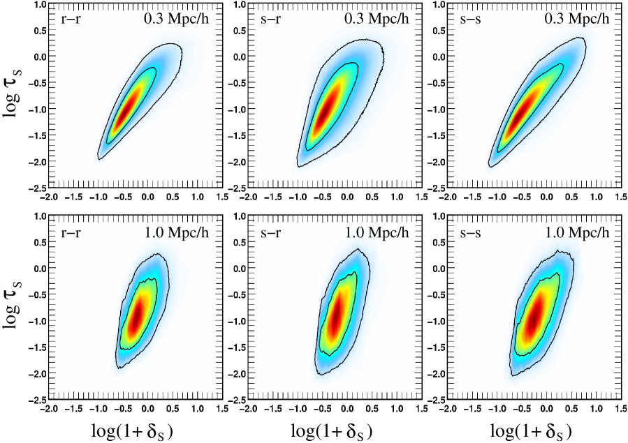
The same trends hold for a smoothing length (lower panels), but in this case the range of densities is compressed, and the correlation is steeper. As a result, the scatter in optical depth has larger impact relative to the trend with density. For our calculations below, we have experimented with a range of smoothing lengths, and we find that the best results (i.e., the most accurate predictions for flux statistics) are obtained with a smoothing length in the range . This is comparable to the Jeans scale for (Peeples et al., 2010) and somewhat smaller than the BOSS spectra resolution scale of . We have not tested whether smaller smoothing lengths would give better results for higher resolution spectra. However, we also carry out most of our tests for smoothing, as this still works quite well, and it can be applied to N-body simulations with lower resolution.
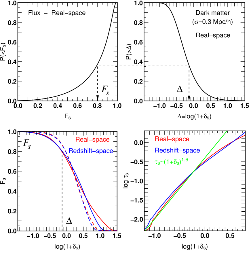
The FGPA converts DM density to optical depth using a physical model motivated by photoionization equilibrium assuming that all gas contributing to the LyaF lies on a temperature-density relation , leading to This relation makes sense for modeling high-resolution spectra, but it does not necessarily apply at low resolution because of the non-linear relation between flux and optical depth, and even in the high-resolution case it omits some physical effects. Alternatively, one can derive an “optimal” deterministic relation between smoothed density and smoothed flux that is calibrated on hydro simulations, a strategy advocated by Gallerani et al. (2011). A straightforward choice for an “optimal” mapping is to find the unique monotonic relation between the smoothed matter density and the smoothed flux such that the spectra generated from the dark matter have the same unconditional 1-point flux PDF as the spectra from the hydro simulation. We do so by matching the corresponding cumulative distributions to a pixel with DM contrast we assign a flux such that
| (3) |
where and are the 1-point PDFs of flux and DM density measured from the simulation. Figure 5 illustrates this procedure graphically and shows the resulting mapping, which is slightly different in real space and redshift space because the PDFs are different in the two cases (see Fig. 3). The mapping is also different if we consider the DM smoothing rather than the smoothing. Well after reionization, the interplay between photoionization heating and adiabatic cooling produces a temperature-density relation in the diffuse photo-ionized medium that dominates the LyaF (Katz, Weinberg, & Hernquist, 1996; Hui & Gnedin, 1997), and in this case (which applies in our simulation) the FGPA predicts . Our deterministic relations for smoothing have this logarithmic slope at low density, but the relation flattens somewhat at higher density, with lower optical depth than the extrapolation predicts. This flattening may be partly a consequence of working at BOSS resolution rather than high resolution. We will use the deterministic mappings plotted here as a foil for evaluating the success of the LyMAS probabilistic scheme.
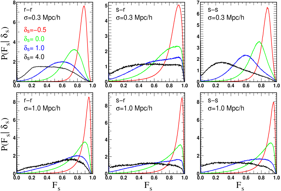
The scatter in Figure 4 shows that the relation between DM density and flux is not, in fact, deterministic. Figure 6 plots the conditional probability distributions for dark matter density contrasts , 0, 1, and 4; each curve represents a vertical cut through the corresponding panel of Figure 4. Beginning with the top row, for DM smoothing length , we see that these conditional distributions are quite broad, though they always show the expected trend of lower average flux for higher DM density. The middle panel, based on redshift-space spectra but real-space DM densities, has broader distributions as expected. However, when we use redshift-space DM densities (right panel), the distributions are if anything sharper and more differentiated than those obtained for real-space spectra and real-space DM densities (left panel). The bottom row, for DM smoothing , shows similar trends, but the curves are less differentiated than those for . The distributions for , 0, and 1 have maxima at nearly the same flux level ( in the right panel), and in redshift-space the curve is nearly flat over a wide range of flux, so its maximum is poorly defined. This difference is not surprising, since the smoothing scale is larger than the BOSS spectral resolution scale, and smoothing the DM density to this scale therefore loses information that is relevant to predicting the BOSS-resolution flux. We will nonetheless find that the LyMAS scheme with DM smoothing outperforms the deterministic scheme with smoothing.
As described already in the introduction, the philosophy of LyMAS is to assume that the fluxes along separate lines of sight can be drawn independently from the conditional probability distributions , with the flux correlations across lines of sight arising from correlations in the underlying DM density field (coherent fluctuations in the UV background or the IGM equation-of-state could also produce large scale flux correlations; these effects can be incorporated into LyMAS simulations, but we have not done so here). To compute 2-point flux statistics via LyMAS, we create artificial spectra along each of the DM skewers extracted from the simulation, assigning to each pixel a flux that is randomly drawn from the conditional distribution that we have computed from the hydro simulation and illustrated in Figure 6. The creation of artificial spectra is not strictly necessary for computing these flux statistics; it is effectively a convenient Monte Carlo method of doing the relevant integrals over the probability distributions. As discussed in §4 below, the artificial spectra created in this simple manner are unrealistic because they ignore additional correlations (beyond those from DM alone) that arise in neighboring pixels along a single line of sight. In §4 we present a method for creating realistic artificial spectra that have the correct degree of coherence along individual lines of sight, but this more complex method is not needed for predicting flux statistics in the idealized case, with no contribution from observational effects such as noise and continuum fitting errors.
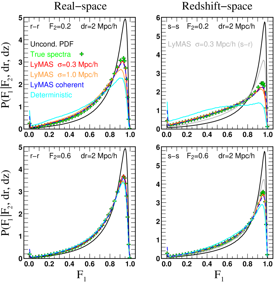
Figure 7 plots conditional PDFs for fluxes of pixels at the identical redshift along lines of sight with transverse comoving separation of : is the probability of finding flux given that the pixel at , has flux (top panels) or 0.6 (bottom panels). In practice, we compute these distributions for pixels with or . Left panels show the case with spectra and DM densities both computed in real space (i.e., with all peculiar velocities set to zero), and right panels show the case with both spectra and density fields computed in redshift space. In each panel, the solid black curve shows the unconditional 1-point PDF. As expected, imposing the condition , i.e., strong absorption along the neighboring line of sight, increases the probability of being low. The peak of the conditional distribution is depressed in amplitude, but it is only slightly shifted in location relative to the unconditional PDF. Interestingly, the impact of the condition is stronger in redshift space than in real space, presumably reflecting the additional effects of coherence in the velocity field. For , which still represents fairly strong absorption (about 15th-percentile in the cumulative distribution), we see similar effects but reduced in magnitude.
Even for this fairly small transverse separation, the LyMAS scheme with reproduces the results from the true hydro spectra555We hereafter refer “true hydro spectra” or “true spectra” to as spectra derived from the MareNostrum hydro simulation. almost perfectly, with the most noticeable error being a small deviation in the height of the peak. The deterministic scheme is considerably less accurate, especially in redshift space and for the lower . Remarkably, despite the broader conditional distributions seen in Figure 6, LyMAS with is nearly as accurate as with when computing the conditional flux PDF at these separations, and it is again much more accurate than the deterministic relation. The blue-dashed curve in all panels shows results for the “coherent” pseudo-spectrum method described in §4; for now, we simply note that they are essentially identical to those from our “minimal” LyMAS scheme with the same DM smoothing length. Grey curves in the right panels show the effect of using the real-space DM density to predict the redshift-space flux. The performance is much worse than using the redshift-space density field, as expected given our previous results. For all future plots, we will use only the redshift-space hydro spectra and the redshift-space DM density fields.
We note that all four of the schemes shown in Figure 7 reproduce the unconditional 1-point PDF of the true spectra by construction, up to tiny statistical fluctuations associated with the finite number of spectra that we have created.
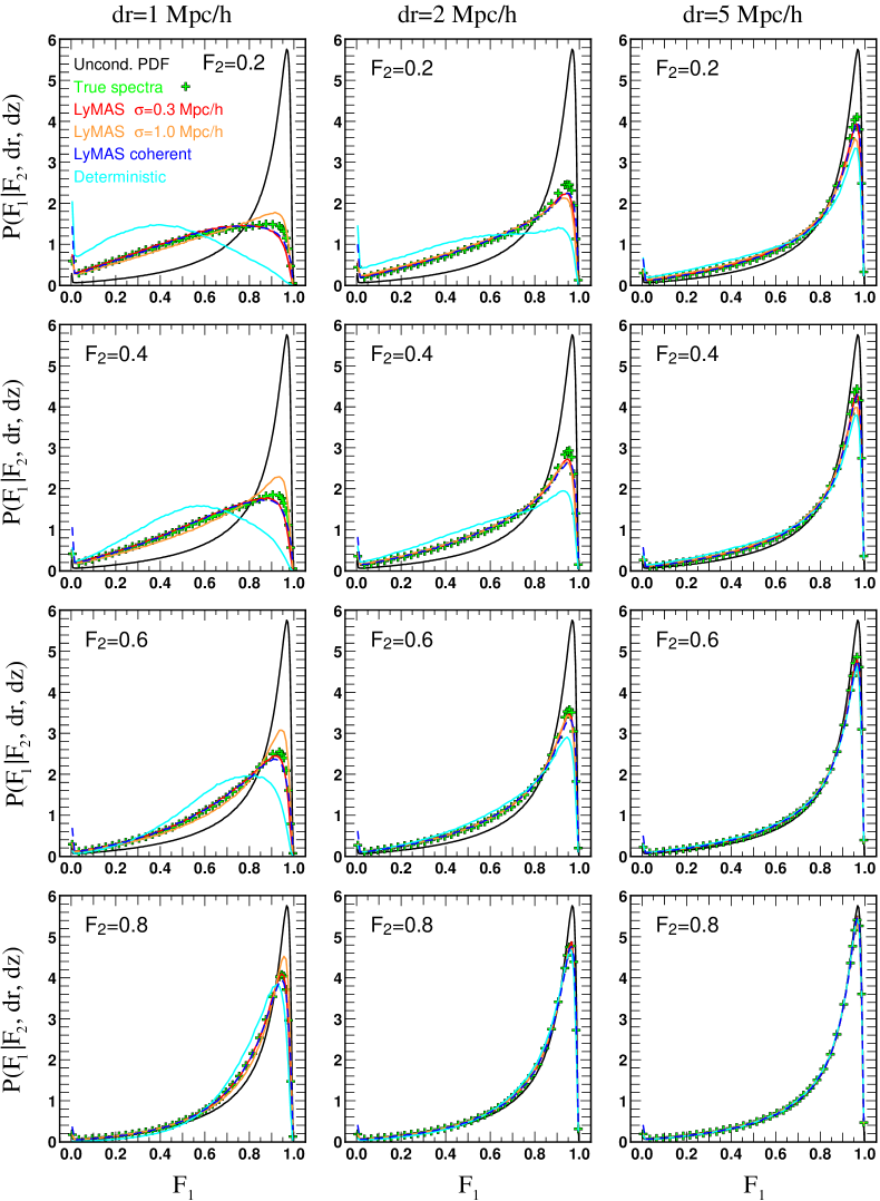
Figure 8 presents a broader view of the the conditional flux distributions. We now consider three different transverse separations, , 2, and , and four different conditioning flux values, , 0.4, 0.6, and 0.8. Two of the panels in the middle column repeat the two right-hand panels of Figure 7. We can see a number of trends, all in qualitative agreement with expectations. The impact of the conditioning flux is strongest when the transverse separation is small, though it is still noticeable at . As the conditioning flux is increased, the conditional PDF of shifts towards higher flux values. For and , the conditional PDF nearly matches the unconditional PDF. LyMAS predictions are more accurate than those from the deterministic scheme in every case, though the difference becomes smaller as the conditional PDF approaches the unconditional PDF. For , LyMAS is impressively accurate even for a transverse separation . For , the predictions are noticeably less accurate at than at , though still much more accurate than those of the deterministic scheme. The coherent spectrum method of §4 gives results that are essentially indistinguishable from those of the minimal LyMAS in all cases.
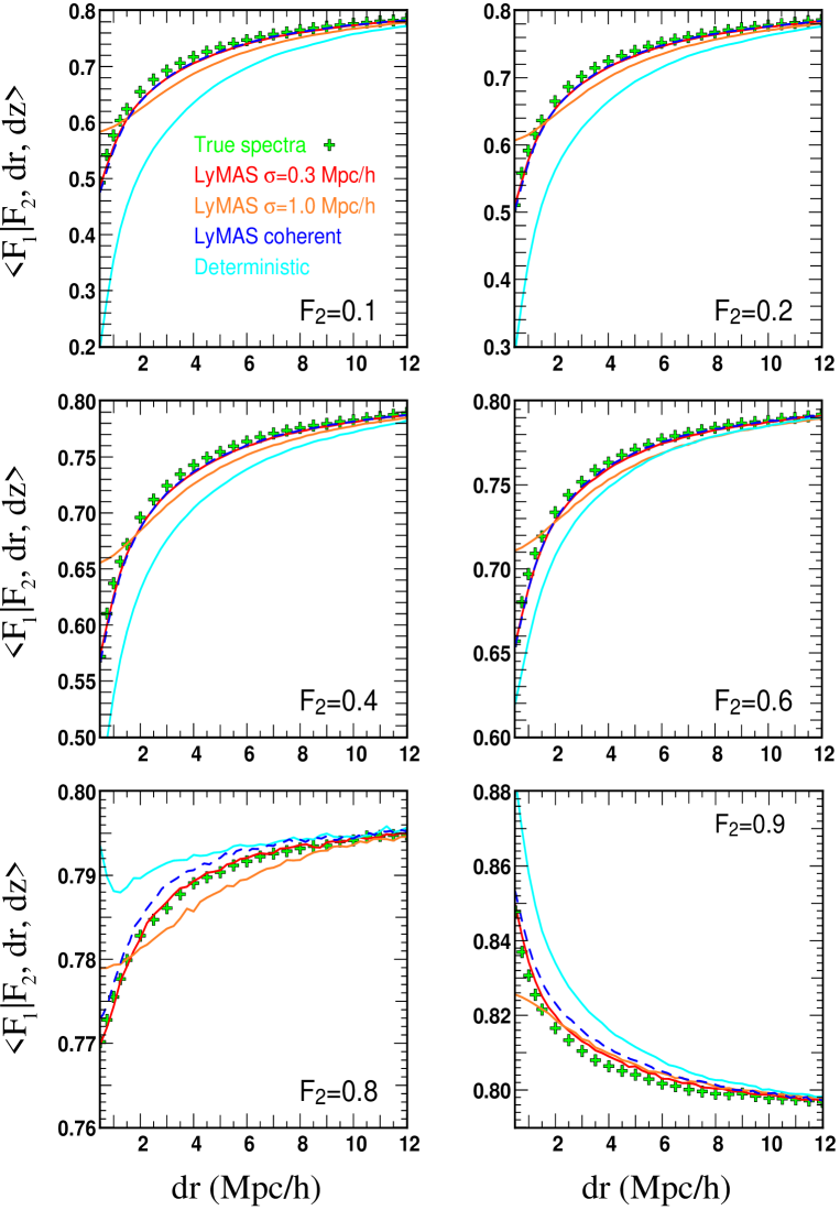
Conditional distributions like those in Figure 8 provide a comprehensive description of the two-point correlations in the LyaF flux field. However, they are difficult to measure from spectra with significant noise, since the underlying flux PDFs are convolved with the noise distribution. Figure 9 shows a higher-level summary statistic, the conditional mean flux , plotted as a function of transverse separation for various choices of the conditioning flux . The effects of noise on the PDF of should average to zero when computing the conditional mean, making this a more easily measurable statistic (it also requires fewer lines of sight to give a useful measurement). However, a proper comparison to observations would have to account for the effects of noise on the conditioning flux , which do not cancel by averaging; we ignore these effects here. Note that the vertical scales are different in each panel. As expected, the conditional mean flux approaches the unconditional mean at large , and it dips (or, in the case of , rises) towards the value of for small transverse separation. Starting from the value at , the conditional mean has typically recovered about halfway towards the unconditional value by . LyMAS with reproduces the results from the true hydro spectra accurately in all cases even down to . It is substantially more accurate than the deterministic scheme, which tends to strongly overestimate the impact of the condition at small transverse separations. With the finer discrimination allowed by this summary statistic, we see that the smoothing length makes LyMAS noticeably less accurate even at separations of , though the largest discrepancy arises at , and even with the larger smoothing length LyMAS is almost always more accurate than the deterministic scheme computed with the optimal smoothing length.
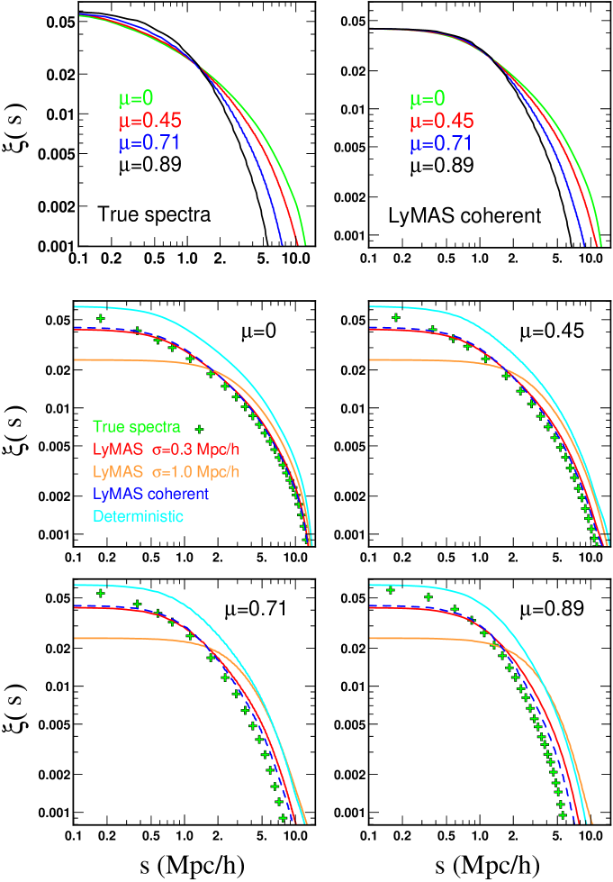
Finally, Figure 10 shows the variations in redshift space of the correlation function as a function of the separation and angle defined for a pair of pixels (, ) by , where and the component along the line of sight. In the present case, we have considered four distinct angles: (i.e. ), (), () and (). Again, we find that results obtained from the coherent LyMAS scheme with are in good agreement with those from the true hydro spectra apart from very small separations () where LyMAS tends to underestimate the correlation function computed from the true spectra. As shown in the top panels, the -dependence of is quite strong, the signature of redshift-space distortions in the Ly forest. This effect is seen in the observational analysis of BOSS spectra by Slosar et al. (2011). With , LyMAS predicts this redshift-space distortion accurately, though it performs somewhat worse at high values of . With , LyMAS overpredicts at large and , though it outperforms the deterministic scheme for . It is perhaps somewhat surprising that the discrepancy persists at large , a point that would be useful to revisit with hydro simulations of a still larger volume. The trends in Figure 10 agree qualitatively with those found by Slosar et al. (2011) in BOSS (their figure 17), but quantitative assessment will require reproducing the continuum removal method of Slosar et al., and it probably requires a larger box to accurately represent large scale flows.
4. Creating Pseudo-Spectra
As presented in §3, LyMAS is a tool for predicting flux statistics from a dark matter distribution, not for creating realistic artificial LyaF spectra. However, it is often useful to create such artificial spectra so that one can assess the impact of noise, continuum fitting errors, and other aspects of the observational analysis, and incorporate any biases from these effects into the model predictions before comparing to observations. In this Section we develop a method for creating “pseudo-spectra” with realistic line of sight properties that also have accurate large-scale, 3-d correlations like those predicted by LyMAS.
Figure 11 illustrates the challenge. In the upper panel, the black curve shows the true LyaF spectrum along a line of sight through the hydro simulation. The red curve shows the result of taking a skewer through the smoothed DM density field along the same line of sight, then drawing flux values at each pixel from our calibrated conditional distribution . This curve is much “noisier” than the true spectrum because the LyMAS assumption that separate pixels are represented by independent draws from this conditional distribution obviously breaks down when we are examining neighboring pixels along the same line of sight. The second panel of Figure 11 demonstrates this point explicitly by plotting the “percentile spectrum”: for each pixel, we plot the fractional position of the flux value in the true hydro spectrum in the cumulative distribution of . Specifically, for a pixel with smoothed flux and smoothed redshift-space density , we plot
| (4) |
(To truly make this a “percentile” spectrum we should multiply by 100, but we instead retain the more natural normalization so that runs from zero to one.) We see from Figure 11 that when one pixel has a high value of , and thus a high flux relative the conditional mean expected given the local DM density, then its neighboring pixels also have high values of . The coherence of the “percentile field” dies away gradually with separation, but independent draws from lose this coherence entirely.
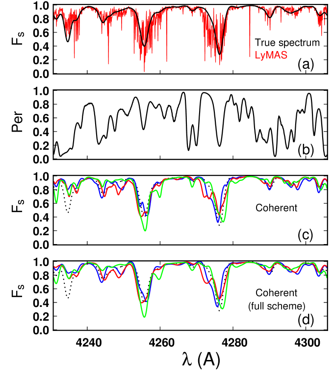
Figure 11 also suggests a strategy for creating more realistic pseudo-spectra: for each skewer through the smoothed DM density field (where represents redshift-space position along the line of sight), first generate a percentile spectrum with the correct statistical properties, then draw the flux in each pixel from the conditional distribution at the location in this distribution implied by . The dotted curves in Figures 12a and 12b show, respectively, the line of sight autocorrelation function of and its Fourier transform, the 1-d power spectrum, both computed from the full set of 100,000 spectra from the hydro simulation. Here we have subtracted the mean and divided by the standard deviation to create a normalized field. The normalized autocorrelation function drops rapidly from 1.0 at zero separation to 0.1 at , then drops slowly towards large separations. The power spectrum is approximately flat from (the fundamental of the box) up to , then drops rapidly at higher .
To create percentile spectra, we first Gaussianize , applying a monotonic mapping that preserves the rank order of pixel values but imposes a Gaussian 1-point PDF — i.e., we replace with
| (5) |
Gaussianization was introduced by Weinberg (1992) as a method to map the present-day galaxy density field back to cosmological initial conditions, and it was introduced for LyaF analysis by Croft et al. (1998). In our case, it ensures that the field has a Gaussian 1-point PDF, though it does not ensure that is actually a Gaussian field, which requires all multi-point PDFs to be multi-variate Gaussians. Note that we apply the Gaussian mapping collectively to the full ensemble of percentile spectra extracted from the hydro simulation, not one line of sight at a time. By construction, has zero mean and unit standard deviation. Solid curves in Figures 12a and 12b show the autocorrelation function and 1-d power spectrum of this Gaussianized percentile field. They differ only moderately from those of itself.

For any dark matter skewer, we can now generate a Gaussian field with same 1-d power spectrum as in the usual way, by drawing the real and imaginary parts of each Fourier mode from independent Gaussian distributions with variance , enforcing the Hermitian condition , and Fourier transforming to get a real-valued field (We use lower case to distinguish these realizations of Gaussian fields from the original Gaussianized field derived from the hydro simulation). After generating fields for an ensemble of skewers, we “de-Gaussianize” them to create a realization of a percentile field along each line of sight — i.e., we monotonically map the values of to match the uniform PDF that by definition describes a percentile field. (We again use lower case to distinguish our realization of from the field measured from the hydro simulation.) Finally, we create an actual spectrum along each line of sight by drawing the smoothed flux from at the location in the cumulative PDF implied by the realization , assigning each pixel the value of satisfying
| (6) |
This procedure is reasonably successful. The third panel of Figure 11 shows three realizations of spectra from this procedure along the same line of sight, which can be compared to the true spectrum in the top panel. The three realizations differ only in the random number seed used to generate . In contrast to the red curve in the top panel, these pseudo-spectra all display a coherence similar to that of the true spectrum. In an ensemble of pseudo-spectra, the values of will still be uniformly distributed, and we will therefore sample fairly from despite introducing correlations to our draws for pixels along the same line of sight. By construction, therefore, an ensemble of pseudo-spectra created in this way has the same 1-point PDF as the original hydro spectra and makes the same predictions for the two-point conditional flux PDFs and flux correlation functions as the LyMAS scheme described in §3. (We have confirmed numerically that we do indeed get identical results from the two approaches, up to statistical fluctuations from the finite number of spectra.) We emphasize that this procedure is not the same as simply generating Gaussian fields and monotonically mapping them to the flux PDF of the original hydro spectra, as that approach would not use the information in the dark matter skewers along each line of sight and would therefore not build in large scale correlations.
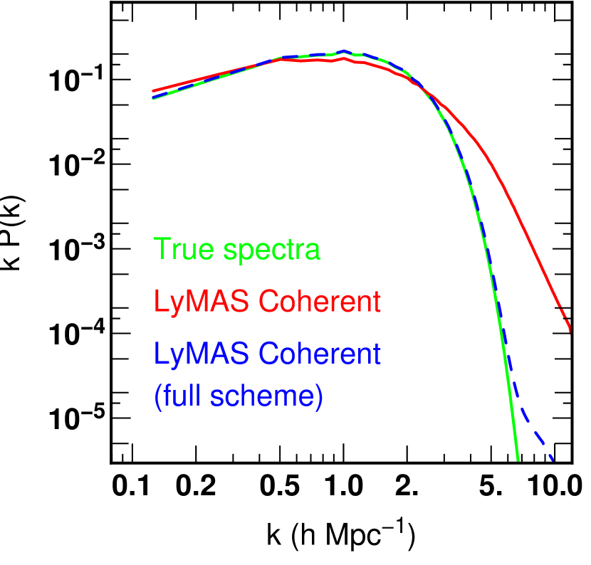
Unfortunately, the 1-d power spectrum of pseudo-spectra generated in this way is not a perfect match to the 1-d power spectrum of the original hydro spectra. Figure 13 shows this comparison, demonstrating that the pseudo-spectra have more power on small scales and slightly less power on large scales; they are not quite coherent enough. To solve this problem we borrow a scheme from Weinberg & Cole (1992), who were attempting to create non-Gaussian fields with specified power spectra via local transformations of Gaussian fields. In our case, we have a well-defined target power spectrum — that of the ensemble of true hydro spectra — and we have a set of pseudo-spectra whose 1-d power spectrum deviates from the target , primarily at high . We repair the discrepancy by computing a 1-d Fourier transform of each pseudo-spectrum, multiplying each Fourier mode by the ratio , and inverse transforming. The ensemble of modified pseudo-spectra now has the same average 1-d power spectrum as the original hydro spectra, by construction.666We use the values of and computed from the ensembles of hydro spectra and pseudo-spectra, so that we do not artificially force the 1-d power spectrum of each individual skewer through the simulation box to match the same global power spectrum. As noted by Weinberg & Cole (1992), this power spectrum modification alters the 1-point PDF, but the change is small. For our purposes, we would like to have spectra that have both the correct 1-d power spectrum and the correct 1-point PDF, and we therefore apply one more monotonic transformation to the fluxes of the pseudo-spectra to match the 1-point PDF of the hydro spectra. This transformation slightly alters the 1-d power spectrum, and in principle one could iterate back and forth between these two steps. In practice, we find that a single iteration already produces excellent agreement with the target 1-d power spectrum up to quite high , as shown by the dotted curve in Figure 13. The 1-point PDF is perfect by construction. We therefore stop after this single iteration. We emphasize that our procedure imposes a global match to the hydro simulation’s flux PDF and 1-d but does not impose this match spectrum-by-spectrum; each individual spectrum has the expected random fluctuations about the global mean statistics.
In Figures 7-10 we have shown the quantitative predictions of this “coherent” LyMAS scheme with blue dashed curves, and they are almost indistinguishable from those of the simpler procedure described in §3. Therefore, our more elaborate procedure provides a method to create ensembles of pseudo-spectra that have the same 1-d power spectrum and 1-point PDF as those from the hydro simulation and that accurately reproduce the predicted cross-sightline correlations for transverse separations larger than . Note that we have also verified that the coherent scheme with smoothing generates results similar to the simple scheme with .
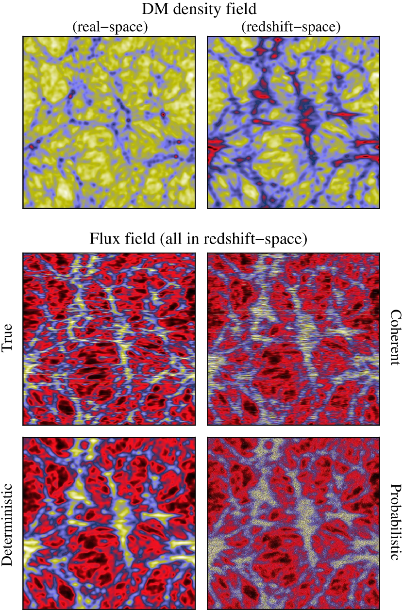
Figure 14 illustrates the relation between the DM density field and the “flux field” that could in principle be measured on an extremely high density grid of LyaF sightlines. Upper panels show slices through the density field in real space and redshift space, smoothed with . Lower panels show the flux field in the same slice computed using the true gas distribution of the hydro simulation, using the deterministic mapping or the simple LyMAS scheme (here labeled “probabilistic”) described in §3, or using the coherent scheme described in this section. It is visually apparent that the true flux field resembles the redshift-space density field more than the real-space density field, as one would expect. In this large scale view, the differences among the three flux assignment schemes are subtle, though one can see that the probabilistic scheme loses some of the fine structure in the true flux field because of its incoherent sampling of .
We close this section with a technical recap of the full LyMAS recipe for creating an ensemble of pseudo-spectra from a dark matter simulation. The inputs needed from the hydro simulation are: 1. The conditional flux distributions for whatever 3-d smoothing length will be applied to the DM simulation. For BOSS resolution spectra, we find that is an optimal choice, but still yields good results for transverse separations above . 2. The 1-d power spectrum and unconditional PDF of the hydro spectra. 3. The 1-d power spectrum of the Gaussianized percentile spectra . In the website dedicated to LyMAS, we provide tabulations of these quantities derived from the RAMSES simulation so that others can use these calibrations to create pseudo-spectra from their own DM simulations.
With these inputs, the steps for creating pseudo-spectra are: 1. Extract skewers through the smoothed DM density field. Our tests in this paper are based on the fairly sophisticated smoothing scheme described in §2, and we have not tested whether simpler methods give adequate results. 2. For each DM skewer, create a realization of a 1-d Gaussian field with the hydro-calibrated power spectrum of . The computed from our hydro simulation necessarily cuts off at , but the coherence scale of is clearly much smaller than this, about in the autocorrelation function (Fig. 12), so we recommend smoothly truncating the power to zero for the lower values that arise in larger simulations. 3. Along each skewer, create an initial flux field by drawing the flux at each pixel from the location in implied by the value of (eq. 6). 4. Measure the 1-d flux power spectrum of the ensemble of pseudo-spectra created in this way. Then Fourier transform each pseudo-spectrum, multiply each of its Fourier components by the ratio , and inverse transform to get modified pseudo-spectra that have the same 1-d flux power spectrum as that from the true hydro spectra. 5. Monotonically map the flux values of so that their unconditional PDF matches that of the hydro spectra, obtaining the final realization of the smoothed flux spectra .
While one could iterate steps 4 and 5, in our test the final monotonic mapping barely alters the 1-d flux power spectrum, so an iteration is unnecessary. For some purposes, one may prefer pseudo-spectra calibrated to match observations rather than representing the prediction of a theoretical model. In this case, one could use empirical estimates of the flux power spectrum and unconditional PDF in place of the hydro simulation results in steps 4 and 5, while still using the DM simulation to build in realistic large scale flux correlations. One could potentially use an approximate method in place of an N-body simulation to generate the redshift-space DM density field, such as a log-normal transformation of a linear theory, Gaussian realization. One caveat is that this density field will not have the same density PDF as that of the hydro simulation used for calibration, so the pseudo-spectra created in step 3 will not have the correct flux PDF. The results after steps 4 and 5 may still be good, but we have not tested such a case.
5. Application to large cosmological dark matter simulations
In this section we apply our full LyMAS recipe for creating an ensemble of pseudo-spectra from a large volume dark matter simulation. However, our calibrations of are based on the dark matter distribution of a high-resolution hydro simulation. Two potential complications in applying LyMAS to a larger volume dark matter simulation are that the dark matter in the hydro simulation is affected by gravity of the dissipative baryons and that the PDF of the smoothed dark matter field may be affected by lower resolution. We expect the first effect to be small at the smoothing scales and moderate overdensities relevant to the Ly forest. To address the resolution question we ran several cosmological N-body simulations with Gadget2 (Springel 2005) with different box lengths and similar cosmological parameters to those used in the MareNostrum simulation. We found that the PDF of the smoothed dark matter density contrast agrees well with that from the MareNostrum simulation if the mean inter-particle distance is similar to the considered smoothing length, as illustrated in Figure 15.
In the following, we analyze two cosmological dark matter simulations performed with Gadget2. In order to produce and analyze a reasonable amount of data, each simulation is run with dark matter particles. Thus, to apply our scheme for and , appropriate box lengths are respectively and . Initial conditions have been generated using the MPgrafic code (Prunet et al. 2008). The and simulations start at and , respectively, and end at where we create our ensembles of pseudo-spectra. In each simulation, the Plummer-equivalent force softening adopted is 5% of the mean inter-particle distance ( and respectively), kept constant in comoving units. We generate redshift-space dark matter density fields on a grid. While the PDFs of are already close to those obtained from the hydro simulation (Figure 15), we monotonically remap to enforce perfect agreement before generating our pseudo-spectra.
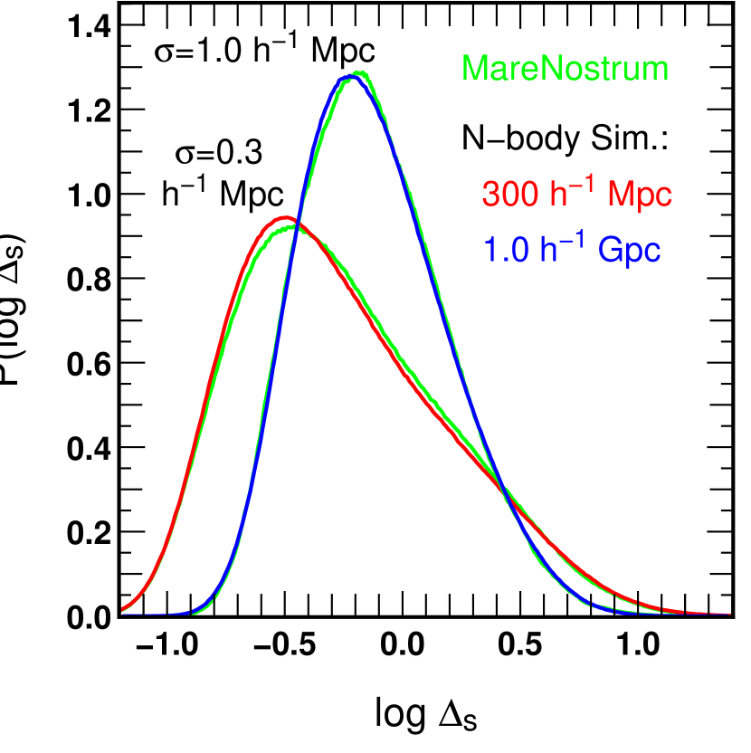
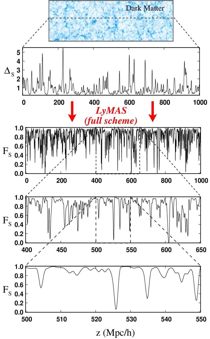
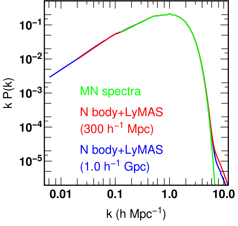
Figure 16 illustrates a pseudo-spectrum through the simulation. The full line of sight has a redshift path length , comfortably larger than the between the Ly and Ly emission lines of a quasar. The lowest, zoomed panel is the same length as a single line of sight through the MareNostrum box, corresponding to an observed-frame wavelength range of 75Å. Figure 17 compares the ensemble-average 1-d power spectrum of the MareNostrum hydro spectra and the LyMAS pseudo-spectra from the and box. By construction, the power spectra agree essentially perfectly over the common range, with the larger boxes continuing out to lower . Because we use only a single iteration, there are discrepancies at , but the power on these scales is too weak to noticeably affect the flux spectra. We have also confirmed that the unconditional flux PDFs of the three sets of spectra match perfectly. Figure 18 shows six spectra extracted from the box at intervals of transverse separation. Across a separation, the coherence of structure along neighboring lines of sight is visually evident. By , there is little coherence still obvious to the eye, though flux statistics do reveal correlations at these scales and larger.
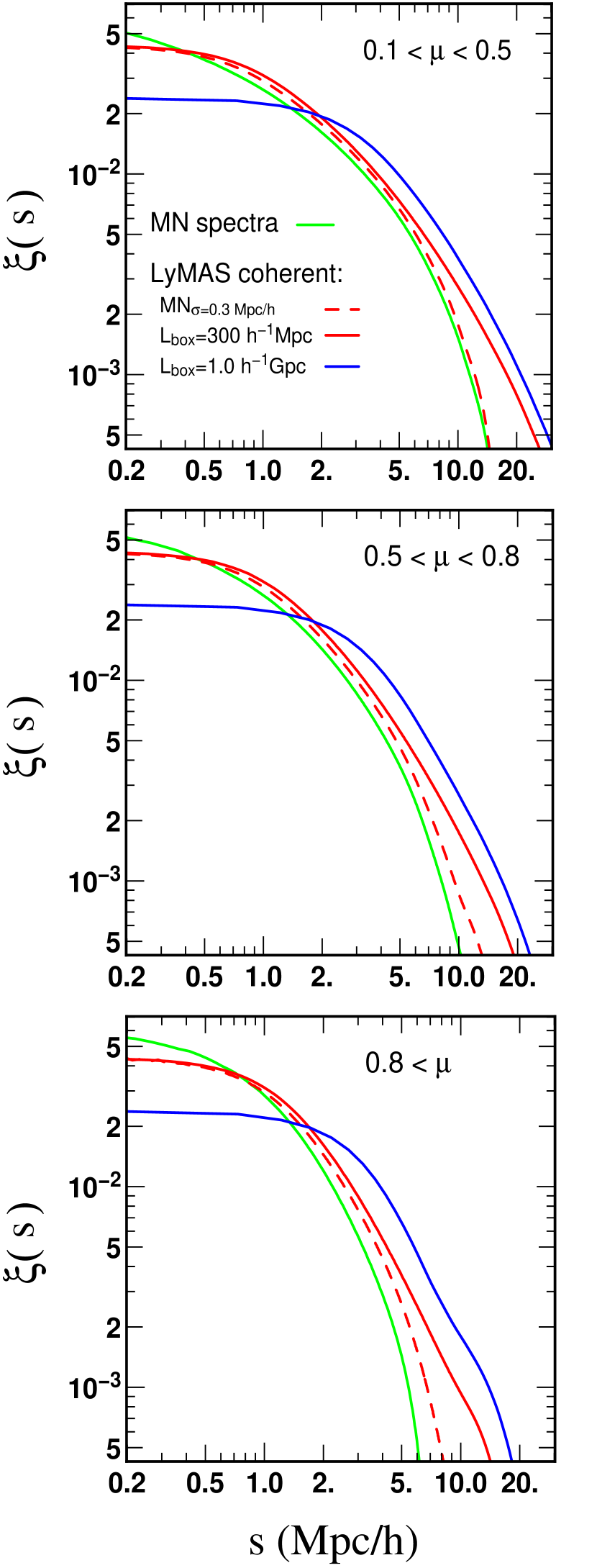
The left panel of Figure 19 shows the correlation functions (3-d, redshift-space) of the smoothed dark matter density fields from the MareNostrum simulation and from the and N-body simulations. The correlation function of the MareNostrum box is noticeably suppressed at and driven to zero at . The correlation functions of the N-body simulations remain positive to . In this plot, the results from the simulation should be the most realistic because they are least affected by cutoff of power at the box scale.
The right panel of Figure 19 shows the redshift-space flux correlation function , averaged over angles and excluding pixel pairs along the same line of sight. The correlation function of the MareNostrum spectra goes negative at , reflecting the behavior of the dark matter correlation function in the left panel. The dashed red line in this panel show the flux correlation function computed from LyMAS pseudo-spectra in the MareNostrum box, with . This accurately tracks from the true hydro spectra, as expected based on the previous results in Figure 10. The red curve shows computed by applying LyMAS to the box, again with ; now remains positive to . The blue curve shows from the box with . While the larger simulation has better representation of large scale power, the predictions are not necessarily more realistic, because smoothing yields less accurate results for than smoothing (Fig. 10), and the smoothing effect is likely more important than the box size effect on these scales. By contrast, the prediction of the simulation is almost certainly more realistic than that of the MareNostrum simulation, as LyMAS with yields accurate predictions of and the box size effects are much weaker for than for .
Dotted and dashed cyan curves in this panel show results from applying the deterministic mapping prescription to the two simulations, with the same smoothing lengths. In each case, the deterministic mapping significantly overpredicts the flux correlation function relative to the more accurate LyMAS scheme, as seen previously for specific values in Figure 10. This difference is not surprising, as the stochasticity in the relation between density and flux should suppress the correlation function of the latter with respect to the former. It is important to take these stochastic effects into account when predicting large scale flux correlations from a cosmological model.
Figure 20 plots the flux correlation function averaged in three broad bins of the angle , defined as described at the end of Section 3. The amplitude of decreases with increasing at fixed , as seen previously in Figure 10. Comparison of the red lines and the dashed red ones shows the influence of box size between the and simulation volumes. As shown previously in Figure 10, LyMAS is less accurate for high values of , indicating some shortcomings at modeling redshift-space distortion for lines of sight with small transverse separations. Nonetheless, the box predictions are likely more realistic than those of the MareNostrum hydro spectra because of the larger simulation volume and the good but not perfect accuracy of LyMAS. The higher amplitude correlation function of the box could be partly due to its larger simulation volume, but comparison to Figure 10 suggests that the dominant effect is the lower accuracy of LyMAS with smoothing.
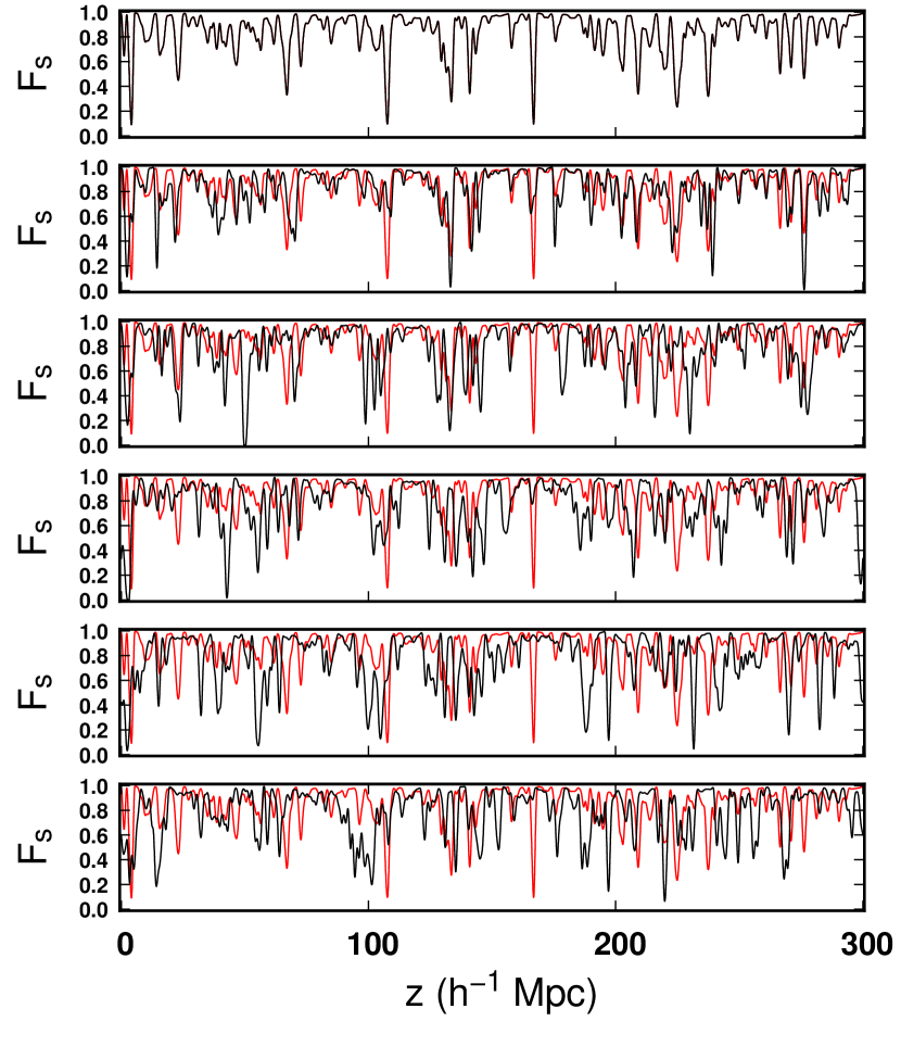
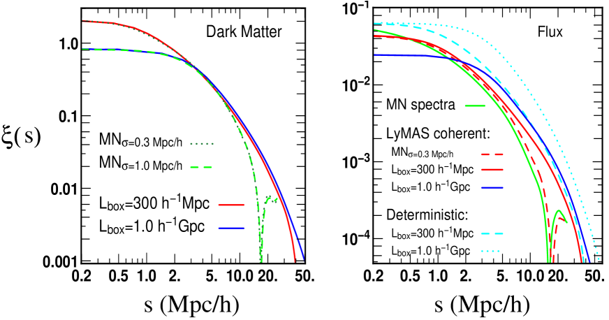
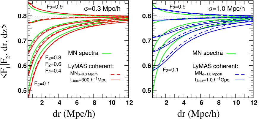
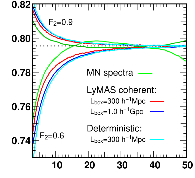
Figure 21 shows the conditional mean flux as a function of transverse separation (with ), for several values of the conditioning flux . As shown previously in Figure 9, LyMAS with reproduces the full hydro predictions for this statistic almost perfectly for in the MareNostrum box. The difference between dashed red curves and red curves in the left panel therefore reflects the larger box size of the simulation, which noticeably increases the signature of flux correlations on this statistic even for as small as . The right panel shows results from the box, but the greater separation between dashed blue and blue curves in this panel likely reflects the lower accuracy of LyMAS with (see Fig. 9). Figure 22 shows the conditional mean decrement at separations , for the and boxes only. The conditional signal has vanished by in the MareNostrum spectra, but in the box it continues out to . Spectra created by deterministic mapping in the box also show this larger scale coherence, but they overpredict the magnitude of the conditional mean effect.
We are making the catalogs of mock spectra from the and simulations publicly available777http://www2.iap.fr/users/peirani/lymas/lymas.htm, as they may be broadly useful for investigating statistics of the 3-d Ly forest. We also make hydro and LyMAS coherent spectra from the MareNostrum box available so that others can look at the accuracy of LyMAS for statistics they are interested in. These spectra are at , and they represent the cosmological model and IGM thermal history used in the MareNostrum simulation. They are smoothed to BOSS spectral resolution, and they are noiseless. We defer the creation of mock spectra that incorporate redshift evolution and noise, and variations of cosmological parameters or IGM parameters, to future work. By construction, these mock spectra reproduce the 1-d flux power spectrum and flux PDF predicted by the MareNostrum hydro simulation. For predictions of 3-d flux statistics, the spectra from the box should yield similar predictions to those that would be obtained from a RAMSES simulation times larger in volume. Predictions from the box suffer from the lower accuracy of LyMAS with smoothing. Nonetheless, these predictions should be significantly more accurate than those from a deterministic flux mapping scheme, and thus from any previous simulation of the Ly forest over such a large volume.
6. Conclusions and Outlook
LyMAS is a promising method for making accurate predictions for flux statistics of the 3-d Ly forest on intermediate and large scales. The underlying idea is that flux correlations on these scales are driven by correlations of the dark matter density field, so that flux statistics can be computed by combining the dark matter density field with the conditional PDF of flux given density, . Here we have calibrated these conditional PDFs using the MareNostrum AMR hydrodynamic simulation, focusing on spectra matched to the resolution of BOSS at . We find the tightest flux-density correlation and the best overall performance of LyMAS for a 3-d dark matter smoothing length (with similar performance down to smaller smoothing lengths of ). The conditional PDFs are quite broad even for this smoothing length, but LyMAS nonetheless gives accurate predictions for the two-point flux distribution and correlations down to transverse separations as small as . It is substantially more accurate than predictions from a deterministic flux-density mapping, even when the latter is optimally tuned to reproduce the unconditional flux PDF of the hydro simulation. Redshift-space distortions have a different impact on the matter distribution and the Ly forest, because mass is conserved under the peculiar velocity mapping while absorption is not. Nonetheless, LyMAS predictions for redshift-space flux correlations from the redshift-space dark matter field prove just as accurate as predictions for the real-space flux correlations (i.e., with peculiar velocities set to zero) from the real-space density field.
For forward modeling tests it is desirable to create artificial spectra that can be analyzed with the same procedures applied to observational data. By forming the “percentile fields” described in §4, we are able to make spectra that are coherent from pixel to pixel along a single line of sight and have the same cross-sightline statistics as the simple LyMAS method in which each pixel flux is drawn independently from . However, the 1-d flux power spectrum of these coherent spectra has more high- power than that measured from the full hydro spectra. By remapping first the amplitudes of Fourier modes and then the pixel flux values, as described in §4, we are able to create model spectra that exactly reproduce the 1-d flux power spectrum and the unconditional flux PDF of the full hydro spectra. The remapping slightly alters the cross-sightline statistics, but they appear to become, if anything, more accurate in reproducing the full hydro results.
For practical purposes it would be useful to adopt larger dark matter smoothing lengths for large scale predictions, so that LyMAS could be applied to lower resolution dark matter simulations of very large volumes. Unfortunately, LyMAS with proves noticeably less accurate than LyMAS with even on scales that are much larger than either smoothing length, tending to overpredict the strength of flux correlations. It is still significantly more accurate than a deterministic mapping, even when the latter is applied at , so LyMAS remains the best method to make mock Ly forest spectra from a low resolution N-body simulation. However, seems required to achieve the full accuracy of the method, which in turn requires an N-body simulation with . We have not investigated whether a smaller dark matter smoothing length would be needed to model high-resolution spectra (from KECK/UVES for instance). We have also not investigated whether larger smoothing lengths would be acceptable, or even preferred, for modeling spectra with lower resolution than BOSS (X-SHOOTER for instance). But in all cases, one would still need to generate new calibrations and new power spectrum of percentile spectra.
LyMAS shifts the problem of simulating Gpc3 volumes of the Ly forest from the realm of computationally impossible to computationally challenging. An N-body simulation of a cube with high enough resolution to produce dark matter skewers requires particles, and even the creation of the dark matter field from the N-body particle distribution is a cpu- and memory-intensive task. One also requires a calibrating hydrodynamic simulation for each cosmological model of interest, of large enough volume to yield accurate . As a first step, we have created catalogs of artificial spectra at BOSS resolution for the MareNostrum cosmology at , from a box with and a box with . In future work, we will investigate methods for incorporating the redshift evolution of the forest over the range probed by an individual quasar spectrum and move towards a full realization (from multiple simulations) of the BOSS quasar sample.
Alongside these technical challenges, the most interesting direction for future study with LyMAS is to explore the sensitivity of medium and large scale structure in the 3-d Ly forest to the underlying cosmological and IGM parameters. Indeed, if the thermal history of the hydro simulation or the cosmological parameters change, the PDF of the flux and then the probabilities would also change. At present, we don’t know if we still need to derive new calibration tables for each set of specific cosmological parameters (or set of thermal history models) or whether a simple rescaling at some steps from the present study would be acceptable. Nevertheless, These investigations can be started by manipulating the MareNostrum simulation to compute conditional flux PDFs for different IGM equations of state (by artificially changing gas temperatures) or matter fluctuation amplitudes (by relabeling output redshifts), then applying these conditional PDFs to different N-body outputs. These rescaling calculations should be spot-checked against fully self-consistent sets of simulations, but we expect they will provide good guidance to the sensitivity of flux statistics to cosmology and degeneracies with the IGM. There are obvious analogies between the LyMAS approach to modeling the Ly forest and methods for creating galaxy redshift catalogs by populating the dark matter halos of N-body simulations in accord with semi-analytic models of galaxy formation, with the advantage that predicting the Ly forest from first principles is more straightforward than modeling galaxy formation. However, the effects of ionizing background fluctuations (Croft, 2004), inhomogeneous reionization (McQuinn et al., 2011), and metal-line contamination remain important potential systematics that require further scrutiny.
The potential payoff from exploiting sub-BAO scales in the 3-d Ly forest is large. One long-recognized opportunity is to apply the Alcock-Paczynski (1979) test to the Ly forest to constrain the product at high redshift (Hui, Stebbins, & Burles, 1999; McDonald & Miralda-Escudé, 1999); this requires accurate predictions of the intrinsic anisotropy in Ly forest clustering. A more model-dependent variant of this idea is to use the amplitude of correlations as a function of transverse separation to constrain directly. The slope and curvature of the matter power spectrum are diagnostics for neutrino masses or curvature in the inflationary fluctuation spectrum, and the Ly forest can probe the power spectrum shape on scales that are degraded by non-linear evolution at low redshift. Most enticing but perhaps most challenging is the prospect of precisely constraining the amplitude of matter clustering at , so that CDM predictions for the growth of structure can be tested from the CMB epoch through the Ly forest epoch down to the lower redshifts probed by large weak lensing and galaxy redshift surveys. These tests could reveal the signatures of complex dark energy models or devations from General Relativity on cosmological scales. With the massively multi-plexed spectroscopic surveys underway and planned for the future, the 3-d Ly forest is emerging as a major new route to tracing the growth of structure in the universe. LyMAS is an important step towards matching theoretical predictions to this observational opportunity.
References
- Alcock & Paczyński (1979) Alcock, C., & Paczyński, B. 1979, Nature, 281, 358
- Angulo & White (2010) Angulo, R. E., & White, S. D. M. 2010, MNRAS, 405, 143
- Bi & Davidsen (1997) Bi, H.G., & Davidsen, A. 1997, ApJ, 479, 523
- Busca et al. (2012) Busca, N. G., Delubac, T., Rich, J., et al. 2013, A&A, 552, A96
- Cen et al. (1994) Cen, R., Miralda-Escudé, J., Ostriker, J.P., & Rauch, M. 1994, ApJ, 437, L9
- Colombi, Chodorowski & Teyssier (2007) Colombi, S., Chodorowski, M. J., & Teyssier, R. 2007, MNRAS, 375, 348
- Croft (2004) Croft, R. A. C. 2004, ApJ, 610, 642
- Croft et al. (1997) Croft, R.A.C., Weinberg, D.H., Katz, N., Hernquist, L., 1997, ApJ, 488, 532
- Croft et al. (1998) Croft, R. A. C., Weinberg, D. H., Katz, N., & Hernquist, L. 1998, ApJ, 495, 44
- Croft et al. (1999) Croft, R. A. C., Weinberg, D. H., Pettini, M., Katz, N., & Hernquist, L. 1999, ApJ, 520, 1
- Croft et al. (2002) Croft, R. A. C., Weinberg, D. H., Bolte, M., Burles, S., Hernquist, L., Katz, N., Kirkman, D., Tytler, D. 2002, ApJ, 581, 20
- Devriendt et al. (2010) Devriendt, J., Rimes, C., Pichon, C., et al. 2010, MNRAS, 403, L84
- Dawson et al. (2013) Dawson, K. S., Schlegel, D. J., Ahn, C. P., et al. 2013, AJ, 145, 10
- Dubois & Teyssier (2008) Dubois, Y., & Teyssier, R. 2008, A&A, 477, 79
- Eisenstein et al. (2011) Eisenstein, D. J., Weinberg, D. H., Agol, E., et al. 2011, AJ, 142, 72
- Faucher-Giguère et al. (2008) Faucher-Giguère, C.-A., Prochaska, J. X., Lidz, A., Hernquist, L., & Zaldarriaga, M. 2008, ApJ, 681, 831
- Font-Ribera, McDonald & Miralda-Escudé (2012) Font-Ribera, A., McDonald, P., & Miralda-Escudé, J. 2012, J. Cosmology Astropart. Phys, 1, 1
- Gallerani et al. (2011) Gallerani, S., Kitaura, F. S., & Ferrara, A. 2011, MNRAS, 413, L6
- Gnedin & Hui (1996) Gnedin, N. Y., & Hui, L. 1996, ApJ, 472, L73
- Gnedin & Hui (1998) Gnedin, N. Y., & Hui, L. 1998, MNRAS, 296, 44
- Greig, Bolton & Wyithe (2011) Greig, B., Bolton, J. S., & Wyithe, J. S. B. 2011, MNRAS, 418, 1980
- Gunn & Peterson (1965) Gunn, J.E., & Peterson, B.A. 1965, ApJ, 142, 1633
- Haardt & Madau (1996) Haardt, F., & Madau, P. 1996, ApJ, 461, 20
- Hernquist et al. (1996) Hernquist L., Katz, N., Weinberg, D.H., & Miralda-Escudé, J. 1996, ApJ, 457, L51
- Hui & Gnedin (1997) Hui, L., & Gnedin, N. 1997, MNRAS, 292, 27
- Hui, Gnedin, & Zhang (1997) Hui, L., Gnedin, N., & Zhang, Y. 1997, ApJ, 486, 599
- Hui, Stebbins, & Burles (1999) Hui, L., Stebbins, A., & Burles, S. 1999, ApJ, 511, 5
- Katz, Weinberg, & Hernquist (1996) Katz, N., Weinberg D.H., & Hernquist, L. 1996, ApJS, 105, 19
- Le Goff et al. (2011) Le Goff, J. M., Magneville, C., Rollinde, E., Peirani, S., et al. 2011, A&A, 534, A135
- Lidz et al. (2010) Lidz, A., Faucher-Giguère, C.-A., Dall’Aglio, A., McQuinn, M., Fechner, C., Zaldarriaga, M., Hernquist, L., & Dutta, S. 2010, ApJ, 718, 199
- McDonald (2003) McDonald, P. 2003, ApJ, 585, 34
- McDonald & Miralda-Escudé (1999) McDonald, P. & Miralda-Escudé, J. 1999, ApJ, 518, 24
- McDonald et al. (2000) McDonald, P., Miralda-Escudé, J., Rauch, M., Sargent, W. L. W., Barlow, T. A., Cen, R., & Ostriker, J. P. 2000, ApJ, 543, 1
- McDonald et al. (2005) McDonald, P., et al. 2005, ApJ, 635, 761
- McDonald & Eisenstein (2007) McDonald, P., & Eisenstein, D. J. 2007, Phys. Rev. D, 76, 063009
- McQuinn et al. (2011) McQuinn, M., Hernquist, L., Lidz, A., & Zaldarriaga, M. 2011, MNRAS, 415, 977
- Miralda-Escudé et al. (1996) Miralda-Escudé J., Cen R., Ostriker, J.P., & Rauch, M. 1996, ApJ, 471, 582
- Miralda-Escudé et al. (1997) Miralda-Escudé, J., Rauch,. M., Sargent, W.L.W., Barlow, T.A., Weinberg, D.H., Hernquist, L., Katz, N., Cen, R. & Ostriker, J.P. 1998, in Proc. of the 13th IAP Colloquium, Structure and Evolution of the IGM from QSO Absorption Line Systems, eds. P. Petitjean & S. Charlot, (Paris: Nouvelles Frontières), p. 155, astro-ph/9710230
- Monaghan (1992) Monaghan, J. J. 1992, ARA&A, 30, 543
- Ocvirk et al. (2008) Ocvirk, P., Pichon, C., & Teyssier, R. 2008, MNRAS, 390, 1326
- Peeples et al. (2010) Peeples, M. S., Weinberg, D. H., Davé, R., Fardal, M. A., & Katz, N. 2010, MNRAS, 349
- Prunet et al. (2008) Prunet, S., Pichon, C., Aubert, D., et al. 2008, ApJS, 178, 179
- Schlegel et al. (2011) Schlegel, D., et al. 2011, The BigBOSS Experiment, arXiv:1106.1706
- Seljak et al. (2005) Seljak, U., Makarov, A., McDonald, P., Anderson, S., et al. 2005, Phys. Rev. D, 71, 3515
- Slosar et al. (2009) Slosar, A., Ho, S., White, M., & Louis, T. 2009, Journal of Cosmology and Astro-Particle Physics, 10, 19
- Slosar et al. (2011) Slosar, A., et al. 2011, JCAP, 9, 1
- Slosar et al. (2013) Slosar, A., Iršič, V., Kirkby, D., et al. 2013, JCAP, 4, 26
- Smee et al. (2012) Smee, S., Gunn, J. E., Uomoto, A., et al. 2012, arXiv:1208.2233
- Sousbie, Courtois, Bryan, & Devriendt (2008) Sousbie, T., Courtois, H., Bryan, G., & Devriendt, J. 2008, ApJ, 678, 569
- Spergel et al. (2003) Spergel, D. N., Verde, L., Peiris, H. V., et al. 2003, ApJS, 148, 175
- Springel (2005) Springel, V. 2005, MNRAS, 364, 1105
- Teyssier (2002) Teyssier, R. 2002, A&A, 385, 337
- Thoul & Weinberg (1996) Thoul, A. A. & Weinberg, D. H. 1996, ApJ, 465, 608
- Viel et al. (2002) Viel, M., Matarrese, S., Mo, H. J., Theuns, T., & Haehnelt, M. G. 2002, MNRAS, 336, 685
- Viel, Haehnelt, & Springel (2004) Viel, M., Haehnelt, M. G., & Springel, V. 2004, MNRAS, 354, 684
- Viel, Haehnelt, & Springel (2006) Viel, M., Haehnelt, M. G., & Springel, V. 2006, MNRAS, 367, 1655
- Viel, Haehnelt, & Springel (2010) Viel, M., Haehnelt, M. G., & Springel, V. 2010, JCAP, 6, 15
- Weinberg (1992) Weinberg, D. H. 1992, MNRAS, 254, 315
- Weinberg & Cole (1992) Weinberg, D. H., & Cole, S. 1992, MNRAS, 259, 652
- Weinberg, Katz, & Hernquist (1998) Weinberg, D. H., Katz, N., & Hernquist, L. 1998, in ASP Conference Series 148, Origins, eds. C. E. Woodward, J. M. Shull, & H. Thronson, (ASP: San Francisco), 21, astro-ph/9708213
- Weinberg et al. (1999) Weinberg, D. H., et al. 1999, in Evolution of Large Scale Structure: From Recombination to Garching, eds. A.J. Banday, R. K. Sheth, & L. N. Da Costa, (Twin Press: Vledder NL), 346 astro-ph/9810142
- White (2003) White, M. 2003, The Davis Meeting On Cosmic Inflation, p. 18, astro-ph/0305474
- White et al. (2010) White, M., Pope, A., Carlson, J., et al. 2010, ApJ, 713, 383
- Zaldarriaga, Hui, & Tegmark (2001) Zaldarriaga, M., Hui, L., & Tegmark, M. 2001, ApJ, 557, 519
- Zhang, Anninos & Norman (1995) Zhang, Y., Anninos, P., & Norman, M.L. 1995, ApJ, 453, L57