The Hunt for Exomoons with Kepler (HEK):
III. The First Search for an Exomoon around a Habitable-Zone Planet

Abstract

Kepler-22b is the first transiting planet to have been detected in the habitable-zone of its host star. At 2.4 $R_{\oplus}$, Kepler-22b is too large to be considered an Earth-analog, but should the planet host a moon large enough to maintain an atmosphere, then the Kepler-22 system may yet possess a telluric world. Aside from being within the habitable-zone, the target is attractive due to the availability of previously measured precise radial velocities and low intrinsic photometric noise, which has also enabled asteroseismology studies of the star. For these reasons, Kepler-22b was selected as a target-of-opportunity by the “Hunt for Exomoons with Kepler” (HEK) project. In this work, we conduct a photodynamical search for an exomoon around Kepler-22b leveraging the transits, radial velocities and asteroseismology plus several new tools developed by the HEK project to improve exomoon searches. We find no evidence for an exomoon around the planet and exclude moons of mass $M_{S}>0.5$ $M_{\oplus}$ to 95% confidence. By signal injection and blind retrieval, we demonstrate that an Earth-like moon is easily detected for this planet even when the time-correlated noise of the data set is taken into account. We provide updated parameters for the planet Kepler-22b including a revised mass of $M_{P}<53$ $M_{\oplus}$ to 95% confidence and an eccentricity of $0.13_{-0.13}^{+0.36}$ by exploiting Single-body Asterodensity Profiling (SAP). Finally, we show that Kepler-22b has a $>95$% probability of being within the empirical habitable-zone but a $<5$% probability of being within the conservative habitable-zone.

1. INTRODUCTION

Kepler-22b is a recently validated extrasolar planet detected by the Kepler Mission via the transit technique (Borucki et al. 2012, B12 hereafter). Orbiting a star with 75% of solar luminosity once every 290 days, Kepler-22b receives an insolation just 10-15% greater than that received by the Earth and thus was claimed to be the first transiting planet discovered to orbit within the so-called habitable-zone of its parent sun (B12). Although habitable-zone exoplanets have been detected by radial velocity surveys (Vogt et al., 2010; Anglada-Escudé et al., 2012), Kepler-22b is a fascinating object thanks to the plethora of follow-up opportunities afforded by transiting planets (Winn, 2010). This excitement is evident in the preceding astronomical literature with speculation about the planet’s habitability (Neubauer et al., 2012), a presently undetected exomoon’s habitability (Heller & Barnes, 2012) and considerable efforts to redefine the so-called habitable-zone (e.g. Kopparapu et al. 2013; Vladilo et al. 2013; Zsom et al. 2013).

Despite the excitement generated by the pioneering discovery of Kepler-22b by B12, the planet cannot be considered “Earth-like” given its radius of 2.4 $R_{\oplus}$. Observationally, the composition of the planet is essentially unconstrained since the upper limit on the planetary mass is quite broad at $M_{P}<82$ $M_{\oplus}$ (2 $\sigma$) (B12). The most well-characterized planet with a radius similar to Kepler-22b would seem to be GJ 1214b (Charbonneau et al., 2009) with a radius of 2.7 $R_{\oplus}$, which has a low bulk density indicating that it cannot have a rock-dominated composition (Anglada-Escudé et al., 2013; Kipping et al., 2013).

Although Kepler-22b may not be a rocky habitable Earth-like world, there is a distinct possibility for the system to yet maintain such a world if Kepler-22b possesses a large moon. Recently, there has been considerable speculation about the potential habitability of such a moon (Heller & Barnes, 2012, 2013) since it is thought that exomoons should be detectable around transiting planets using Kepler (Kipping, 2009a, b; Kipping et al., 2009). Despite this speculation, we note that, to our knowledge, no-one has ever conducted a search for an exomoon in this system. Indeed, we note that there has never even been a search for an exomoon around a habitable-zone candidate planet, let alone a validated one, in the present literature.

The “Hunt for Exomoons with Kepler” (HEK) project (Kipping et al., 2012b) is presently the only systematic program we are aware of attempting to observationally identify extrasolar satellites. Searching for such signals is computationally challenging due to the highly multimodal, complex and high-dimensional parameter space one is faced with (Kipping et al., 2012b), the need for calculating the Bayesian evidence integral (Kipping et al., 2013) and the photodynamic forward modeling required to simulate exomoon signals (Kipping, 2011a). To provide some context, the light curve fits presented in this work required 49.7 years of CPU time. To date, eight Kepler Objects of Interest (KOIs) have been analyzed for evidence of extrasolar moons each with null detections leading to upper limits on the satellite-to-planet mass ratio of $(M_{S}/M_{P})\lesssim 1$-$4$% (Nesvorný et al., 2012; Kipping et al., 2013).

In this work, we present an analysis of the first habitable-zone planet by HEK. This target was identified as a target-of-opportunity by the project because it i) is in the habitable-zone ii) is a validated planet iii) has radial velocity measurements iv) has a quiet, bright ($K_{P}=11.7$) host star v) has a host star with asteroseismology constraints (B12). In this work, we include several new modes to thoroughly explore the exomoon parameter space. These include retrograde (§3.5) and eccentric moon solutions (§3.4), informative and uninformative limb darkening priors (§3.2), applying Bayesian model averaging (§3.10), high-resolution fitting (§3.9), leveraging the radial velocities (§3.7) and asteroseismology constraints (§3.6) and injecting and retrieving synthetic moon signals (§5). We also take this opportunity to provide updated constraints on the mass, radius, composition, habitability and orbit of Kepler-22b using new Kepler data (§4).

2. DATA HANDLING

2.1. Data Acquisition

In the discovery paper of Kepler-22b (B12), three transits were detected by the Kepler Mission occurring in quarters 1, 4 and 7 (Q1, Q4 and Q7). Since this time, an additional three transits should have been observed by Kepler: a $4^{\mathrm{th}}$ transit in Q11, a $5^{\mathrm{th}}$ transit in Q14, and a $6^{\mathrm{th}}$ transit in Q17. The $4^{\mathrm{th}}$ transit was successfully recorded but unfortunately the $5^{\mathrm{th}}$ was not due to a data gap in the Q14 time series. The $6^{\mathrm{th}}$ transit is unlikely to have been recorded because it occurred during a safe mode event from May $1^{\mathrm{st}}$ to May $6^{\mathrm{th}}$ 2013. Further, soon after this Kepler lost functionality of a second reaction wheel on May $12^{\mathrm{th}}$, putting future science observations in doubt. Therefore, it is quite possible that the four transits of Kepler-22b analyzed in this paper will be the only transits ever observed by Kepler. The first transit was observed in long-cadence (LC) mode only, whilst the latter three have short-cadence (SC) data.

We downloaded the reduced data from the Mikulski Archive for Space Telescopes (MAST). In this work, we always make use of the “raw” (labelled as “SAP_FLUX” in the header) data processed by the Data Analysis Working Group (DAWG) pipeline (see accompanying data release notes for details). The “raw” data has been processed using PA (Photometric Analysis), which includes cleaning of cosmic ray hits, Argabrightenings, removal of background flux, aperture photometry and computation of centroid positions. For the sake of brevity, we do not reproduce the details of the PA pipeline here, but direct those interested to Gilliland et al. (2010) and the data release handbooks.

2.2. Detrending with CoFiAM

The Kepler photometry contains several systematic effects which require detrending before a precise transit light curve analysis can be conducted. These effects can be instrumental (such as focus drift, pointing tweaks, safe modes, etc) or astrophysical (such as flaring, rotational modulations, etc). In this work, we utilize the CoFiAM (Cosine Filtering with Autocorrelation Minimization) algorithm described in Kipping et al. (2013) for detrending these various effects.

CoFiAM can be thought of as a high-pass, low-cut periodic filter optimized to undisturb all periodicities at or below the so-called “protected timescale”, $\mathfrak{T}$. The algorithm builds upon initial applications of cosine filtering by Mazeh et al. (2010) for CoRoT photometry and Kipping & Bakos (2011a, b) for Kepler photometry. CoFiAM regresses the following sum of harmonic functions to the time series:

$$F_{k}(t_{i})=a_{0}+\sum_{k=1}^{N_{\mathrm{order}}}\Bigg{[}x_{k}\sin\Big{(}\frac{2\pi t_{i}k}{2D}\Big{)}+y_{k}\cos\Big{(}\frac{2\pi t_{i}k}{2D}\Big{)}\Bigg{]},$$ (1)

where $D$ is the total baseline of the data under analysis, $t_{i}$ are the time stamps of the data, $x_{k}$ & $y_{k}$ are model variables and $N_{\mathrm{order}}$ is the highest harmonic order. For any given $\mathfrak{T}$, one may define the maximum number of distinct harmonic cosines functions ($N_{\mathrm{order}}^{\mathrm{max}}$) to regress to the data without disturbing the timescale $\mathfrak{T}$ as:

$$N_{\mathrm{order}}^{\mathrm{max}} =\frac{2D}{4\mathfrak{T}}.$$ (2)

However, choosing any $N_{\mathrm{order}}<N_{\mathrm{order}}^{\mathrm{max}}$ will also protect the timescale $\mathfrak{T}$. Exploiting this fact, CoFiAM explores every possible variation (in total there are $N_{\mathrm{order}}^{\mathrm{max}}-1$ variations). The detrended light curve after each CoFiAM regression is trimmed to within twice the “window” timescale ($T_{\mathrm{window}}$) of the predicted transit time and then a final linear slope is fitted through the data (excluding the transit itself) to serve as a final normalization.

After every detrending, we compute the autocorrelation on a 30 minute timescale using the Durbin-Watson metric:

$$d =\frac{\sum_{i=2}^{N}(r_{i}-r_{i-1})^{2}}{\sum_{i=1}^{N}r_{i}^{2}},$$ (3)

where $r_{i}$ are the residuals and $N$ is the number of data points. The value of $d$ always lies between 0 and 4, with 2 representing an absence of autocorrelation, $|d-2|>0$ implying otherwise. CoFiAM therefore selects the value of $N_{\mathrm{order}}$ which minimizes $|d-2|$ (hence “autocorrelation minimization”).

CoFiAM is applied to each transit epoch individually and the inputted data is pre-screened for any sharp, discontinuous offsets (due to say a pointing tweak) as well as a general outlier rejection phase using median filtering. We never attempt to stitch two quarters together since there is no reason to expect the detrending function to be smooth between rolls of the spacecraft (which occur every quarter).

In this work, we chose $\mathfrak{T}=3T_{14}$ where $T_{14}$ is the first-to-fourth contact transit duration. Waldmann (2012) showed that $T_{14}$ is the lowest periodicity in the Fourier transform of a transit and so we multiply this by three to provide a small cushion. The “window” timescale is defined to be $T_{\mathrm{window}}=1.2[(T_{14}/2)+T_{\mathrm{Hill}}+T_{14}]$ (the 1.2 factor is again a cushioning factor) where $T_{\mathrm{Hill}}$ is the Hill sphere timescale. For this we define $T_{\mathrm{Hill}}=[M_{P}/(3M_{*})]^{1/3}[P_{B*}/(2\pi)]$ where $P_{B*}$ is the planet’s orbital period, $M_{P}$ is the planet’s mass and $M_{*}$ is the stellar mass. For all of these quantities we simply used the best-fit values quoted in B12 (for $M_{P}$ we used the 3 $\sigma$ upper mass limit).

We stress that the detrending function is regressed independently of the later transit fits. This is done because the form of the detrending function is varied and we typically try between $N_{\mathrm{order}}^{\mathrm{max}}\sim 10$-$30$ different models per transit. To perform the detrending in conjunction with the transits would thus require around $N_{\mathrm{transits}}{{}^{\wedge}}N_{\mathrm{order}}^{\mathrm{max}}$ unique models i.e. $\mathcal{O}[10^{5}]$ for Kepler-22b. Given the very costly compuational demands of even a single photodynamical fit, this would be unrealistic with current computational capabilities.

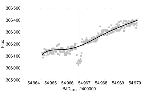
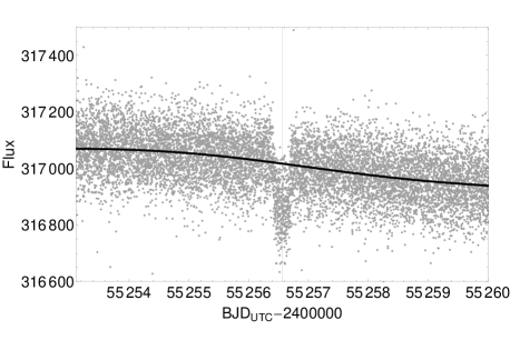
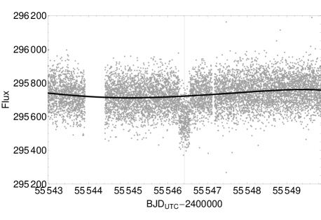
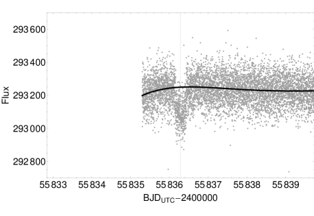
After detrending with CoFiAM, we find $d_{Q1}=1.74069$, $d_{Q4}=1.97479$, $d_{Q7}=1.96775$ and $d_{Q11}=1.86203$ and the detrending functions are plotted over the PA data in Figure 1.

(a) Quarter 1

(b) Quarter 4

(c) Quarter 7

(d) Quarter 11

Figure 1.— “Raw” (PA output) flux observed by Kepler for Kepler-22b. Overlaid is our model for the long-term trend, computed by CoFiAM. Long-cadence data (squares) only is available for Q1 but short-cadence data (dots) is available for the others. The location of the transits are marked with vertical gridlines.

3. MODELING

3.1. Light Curve Fits

We first fit and model the light curve as being due to a single planet transiting the host star, to serve as a benchmark for the subsequent planet-with-moon fits. The planet-only light curve is modeled as was done in Kipping et al. (2013), using the popular Mandel & Agol (2002) algorithm. We assume a quadratic limb darkening law for the host star, where the specific intensity is described by $I(\mu)=1-u_{1}(1-\mu)-u_{2}(1-\mu)^{2}$ where $\mu=\sqrt{1-r^{2}}$, $r$ is the normalized radial coordinate on the stellar disk and $u_{1}$ & $u_{2}$ are the limb darkening coefficients.

Planet-with-moon models are generated using the photodynamic LUNA algorithm (Kipping, 2011a), which inherently accounts for the various timing effects on the planet induced by a moon (Kipping, 2009a, b). We direct the reader to Kipping (2011a) for details on how the photodynamical light curves are computed.

Model light curves are fitted to the data using the multimodal nested sampling algorithm MultiNest (Feroz et al., 2009a, b). By using this code, we not only obtain parameter posteriors but also the Bayesian evidence of each model attempted, thus allowing for later Bayesian model selection and model averaged posteriors. Bayesian model selection is a crucial tool in detecting exomoons due to the roughly doubling of free parameters combined with the complex parameter space (Kipping et al., 2012b).

In general, the methods described above are the same as those implemented in our previous HEK surveys (e.g. see Kipping et al. 2013). Notably, the choice of priors follows that of Kipping et al. (2013) and are shown in Table 1. However, in studying Kepler-22b, we introduced several new changes to our methodology to improve both the accuracy of our derived results and the speed of the computations. These modifications are discussed in what follows.

3.2. Priors for the Limb Darkening Coefficients

In this work, we use two different priors for the limb darkening coefficients: i) informative priors ii) uninformative priors. The informative priors are computed using a Monte Carlo forward modeling of stellar atmosphere models. First, we draw a random normal variate from the effective temperature ($T_{\mathrm{eff}}$) and stellar surface gravity ($\log g_{*}$) and then compute the associated quadratic limb darkening coefficients using the Kurucz (2006) stellar atmosphere model database convolved with the Kepler bandpass (see Kipping & Bakos (2011a) for more details). We repeat this process until $10^{4}$ fair realizations of $u_{1}$ and $u_{2}$ have been computed. For $T_{\mathrm{eff}}$ and $\log g_{*}$, we used the quoted values from B12 of $T_{\mathrm{eff}}=5518\pm 44$ K and $\log g_{*}=4.44\pm 0.06$ but doubled the uncertainties for both.

The $10^{4}$ realizations of $u_{1}$-$u_{2}$ form a joint prior probability for the limb darkening coefficients. For computational expedience, it is desirable to characterize this joint prior probability with a simple analytic form, such as a bivariate Gaussian, rather than calling a stellar atmosphere model at every realization in the light curve fits. However, a bivariate Gaussian is not ideal since our $u_{1}$-$u_{2}$ joint prior probability displays a strong covariance (correlation coefficient of -0.97). Despite this, a bivariate Gaussian can be applied by re-parameterizing the limb darkening coefficients. To this end, we perform a principal components analysis (PCA) on the joint prior probability of $u_{1}$-$u_{2}$ and re-parameterize the terms into the orthogonal components $w_{1}$ and $w_{2}$ following the suggestion of Pal (2008):

$$w_{1} =u_{1}\cos\varphi-u_{2}\sin\varphi,$$

$$w_{2} =u_{2}\cos\varphi+u_{1}\sin\varphi,$$ (4)

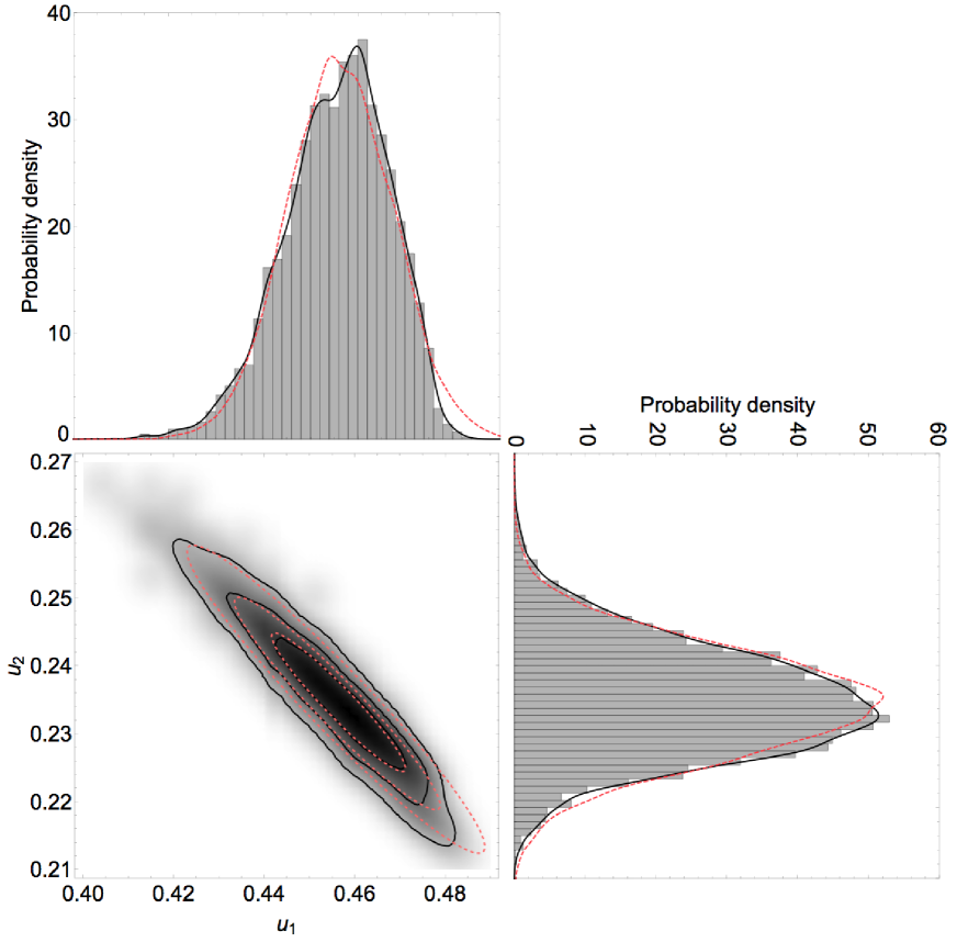
where we derived $\varphi=34.56^{\circ}$ from the PCA. Using this transformation, we computed a joint prior probability for $w_{1}$-$w_{2}$ with negligible covariance. The lack of covariance, combined with the fact the resulting distributions are unimodal and approximately symmetric means that a bivariate Gaussian is now a reasonable analytic approximation. Regressing a Gaussian to each cumulative density function (CDF), we derive normal priors of $\mathrm{P}(w_{1})\sim\mathcal{N}(0.242,0.013)$ and $\mathrm{P}(w_{2})\sim\mathcal{N}(0.45215,0.00070)$. In Figure 2, we compare the PDF in $u_{1}$ and $u_{2}$ predicted by these priors relative to the actual prior probability initially generated, where one can see the good agreement.

Figure 2.— Histograms show the prior probability density distribution of the quadratic limb darkening coefficients $u_{1}$ and $u_{2}$, computed from stellar atmosphere models. In black-solid we overlay the smoothed histogram of the same data. The red-dashed shows the analytic prior probability density function predicted using our $w_{1}$-$w_{2}$ PCA transformed normal bivariate prior probability density function (see §3.2 for details), which serves as an informative prior in the transit fits. The bottom-left panel shows the same as a joint-probability distribution, where the contours represent the 1, 2 and 3 $\sigma$ confidence limits.

The second type of prior we try is an uninformative one. Kipping (2013) recently showed that uniform priors in $u_{1}$-$u_{2}$ can be drawn, without ever sampling unphysical limb darkening coefficients, by applying the “triangular sampling” technique. This is achieved by re-parameterizing the coefficients to $q_{1}$-$q_{2}$ and sampling uniformly between zero and unity in each, where

$$q_{1} =(u_{1}+u_{2})^{2},$$ (5)

$$q_{2} =\frac{u_{1}}{2(u_{1}+u_{2})}.$$ (6)

Employing triangular sampling is approximately twice as efficient than the uninformative priors used previously in Kipping et al. (2013). This is because previously we used uniform priors in $0<u_{1}<2$ and $0<(u_{1}+u_{2})<1$, which spends exactly half of its time sampling from unphysical (and thus rejected) parameter ranges (Kipping, 2013).

3.3. Linear Minimization of Baseline Parameters

In principle, CoFiAM should provide a light curve with an out-of-transit baseline flux equal to exactly unity. In practice, even with CoFiAM’s final stage linear normalization, it is prudent to regress a baseline normalization factor for each transit epoch simultaneous to the transit parameters. One major benefit of doing so is that the uncertainty of the baseline normalization is propagated into the uncertainty of the other transit parameters. In the past, we have treated the normalization factor as a free parameter in MultiNest like any other term. For planets with many transits epochs, this is problematic since the regression now includes a very large number of free parameters leading to laborious CPU times. The fact that a relatively minor nuisance parameter causes this dramatic slow-down makes the situation somewhat impractical.

In this work, we introduce a new refinement to the HEK fitting strategy which simply treats the baseline parameters ($\mathrm{OOT}_{j}$) as a set of nuisance parameters. Rather than marginalizing over these terms, every realization of the transit model simply optimizes the baseline parameters to the data. This is easily achieved using a weighted linear minimization which is both extremely quick and guaranteed to always find the global minimum. In principle, one should wish to marginalize over nuisance parameters rather than simply maximize the likelihood, but in practice we find this procedure has little effect on the other transit parameters and leads to a significant speed-up.

3.4. Eccentricity Caps

Unlike previous surveys, we decided to investigate the potential for eccentric orbits for both the planet and the moon due to the high-priority nature of Kepler-22b. Eccentric fits always require dramatically more time to explore due to i) the introduction of two new free parameters ii) the requirement to solve Kepler’s transcendental equation $\sim$trillions of times during the course of a single fit. Eccentric orbits can also produce unphysical scenarios, unless limits are enforced on the allowed range in $e_{B*}$ (eccentricity of the planet-satellite barycentre around the host star) and $e_{SB}$ (eccentricity of the satellite around the planet-satellite barycentre).

First of all, parameter realizations reproducing collisions should be avoided. We therefore enforce that $a_{SP}(1-e_{SB})>2R_{P}$, i.e. the periastron separation between the planet and the satellite exceeds two planetary radii (we use two planetary radii since the satellite’s radius is $R_{S}<R_{P}$). We use two planetary radii because the satellite’s radius can be up to one planetary radius in our fits. Similarly, for the planetary orbits, we enforce $a_{B*}(1-e_{B*})>2R_{*}$.

Additionally, Domingos et al. (2006) showed that the maximum stable planet-satellite separation is attenuated for eccentric orbits. Domingos et al. (2006) showed that all satellites must conform to:

$$f<0.9309(1-1.0764e_{B*}-0.9812e_{SB}),$$ (7)

where $f$ is equal to the semi-major axis of the satellite relative to the planet in units of the Hill radius. Under the assumption that $M_{S}\ll M_{P}\ll M_{*}$, Kipping (2009a) showed that $f^{3}=(3P_{SB}^{2}/P_{B*}^{2})$, where $P_{SB}$ is the period of the satellite around the planet-satellite barycentre. This allows us to enforce the Domingos et al. (2006) condition as:

$$(3P_{SB}^{2}/P_{B*}^{2})^{1/3}<0.9309(1-1.0764e_{B*}-0.9812e_{SB})$$ (8)

These constraints are optimistic in the sense that the orbits are assumed to be coplanar and the moon is simply a test particle. More realistic solutions can be found by exploring the three-body solution with non-zero masses and three-dimensional geometry (e.g. see Donnison 2010), but we reserve these more detailed dynamical investigations for the final posterior analyses.

We also enforce the same limits on the planet and satellite densities used in Kipping et al. (2013). These various limits are all imposed by simply rejecting any trials reproducing such behavior. Due to the computationally much higher cost of exploring eccentric solutions, we only explored eccentric-planet or eccentric-moon solutions but not both simultaneously, as such fits were found to be prohibitively CPU expensive. Since the Hill stability of a putative moon decreases strongly with increasing eccentricity for both terms, we do not envisage it likely that this significantly hinders our detection ability.

3.5. Retrograde Orbits

In Kipping et al. (2013) we did not explore retrograde orbits for the exomoon, which LUNA defines as being when $180^{\circ}<i_{SB}<360^{\circ}$. In this work, we present a method to explore such orbits whilst still maintaing an isotropic prior in $i_{SB}$. One difficultly in doing this is that an isotropic prior is uniform in $\cos i_{SB}$ but this trigonometric function is not uniquely defined over the interval $0^{\circ}<i_{SB}<360^{\circ}$. For example, $\cos i_{SB}=0$ may refer to $i_{SB}=90^{\circ}$ or $i_{SB}=270^{\circ}$.

Our resolution to this is to introduce an auxiliary cosine term which we dub $\cos^{\prime}i_{SB}$ and is defined over the interval $-1<\cos^{\prime}i_{SB}<+3$. The inverse of this function is given by:

$$i_{SB}=\begin{cases}\cos^{-1}[\cos^{\prime}i_{SB}]&\text{if }-1<\cos^{\prime}i_{SB}\leq+1,\\ \cos^{-1}[\cos^{\prime}i_{SB}-2]+\pi&\text{if }+1<\cos^{\prime}i_{SB}\leq+3.\end{cases}$$

By enforcing a uniform prior in $-1<\cos^{\prime}i_{SB}<+3$ and inverting the above, we reproduce an isotropic prior in inclination and still explore the full range of inclinations (i.e. both prograde and retrograde orbits).

3.6. Asteroseismology Stellar Density Prior

Unlike the previous KOIs analyzed in survey I (Kipping et al., 2013), Kepler-22 has asteroseismology constraints available. Consequently, there exists a strong empirical prior on $\rho_{*}$, the mean stellar density of $\rho_{*}=1.458\pm 0.030$ g cm^-3 (B12). In all fits, we treat $\rho_{*}$ as a normal prior following this measurement.

Usually, the light curve fitted eccentricity and stellar density are highly degenerate but the presence of a strong prior on the latter breaks this degeneracy. This trick was first noted in Kipping et al. (2012a) and was dubbed “Single-body Asterodensity Profiling” by the authors, or SAP. We are therefore able to provide SAP-derived eccentricity constraints in the light curve fits provided in this work.

We also note that B12 are able to combine their precise $\rho_{*}$ measurement with stellar evolution isochrone models to provide precise estimates of the stellar radius and mass ($R_{*}$ and $M_{*}$). Although these are not model parameters in any our fits, we can use them later to derive physical parameters.

3.7. Radial Velocities (RVs)

As part of the campaign to validate the planetary nature of Kepler-22b, B12 obtained sixteen high resolution spectra of the target star between 17 August 2010 and 25 August 2011 using the HIRES spectrometer on the Keck I 10 m telescope, which we utilize in this work. The spectra yield $\sim 1.4$ m s^-1 precision radial velocities and show no clear detection of Kepler-22b. The null-detection is consistent with a low-mass planet, as expected for the radius of Kepler-22b. By leveraging these radial velocities, we can constrain various parts of the parameter space explored by MultiNest, such as excluding massive planets or moderate-mass planets on highly eccentric orbits.

Including the RVs requires only two extra free parameters to our model, $K$ and $s$ (the radial velocity jitter), since all of the other orbital parameters are included in our fits anyway. The jitter term behaves like an additional error which is simply added in quadrature to the reported RV uncertainties. Unlike B12, we do not choose a fixed $s$ value of $3$ m s^-1 but rather we fit the parameter using a modified Jeffrey’s prior, as advocated by Balan & Lahav (2009). Following Balan & Lahav (2009), we choose the inflection point of the modified Jeffrey’s prior to be equal to the median RV uncertainty and set the maximum to be equal to twice the range of the reported RVs. The same prior is also used for $K$.

The radial velocities can be used to derive the planetary mass, $M_{P}$, given a known stellar mass, $M_{*}$. To determine $M_{P}$, we solve the cubic equation of the well-known mass-function using Equation 3.18 of Kipping (2011b). Whilst some authors, such as B12, have advocated exploring negative $K$ solutions to avoid positive-biases in fitting joint RV + transit data, this is actually unnecessary for MultiNest as the nested sampling technique does not suffer boundary condition biases, unlike Markov chains.

3.8. Negative Radii Moons

A new feature we implement in this work for the HEK project is the exploration of negative $(R_{S}/R_{P})$ solutions i.e. negative radii moons. Negative radii moons are of course not physically plausible and our implementation simply involves flipping the transit signal component caused by the moon in such cases. We exploit this trick as a vetting test such that solutions favoring a negative radius moon can be easily dismissed. This replaces the previous test of Kipping et al. (2013) of fitting for zero-radius moons and comparing the Bayesian evidence. We find that negative-radius moon exploration is more efficient computationally since we do not require another additional moon fit purely for vetting purposes. We select a uniform prior on the radius ratio term of $-1<(R_{S}/R_{P})<+1$.

Table 1Planet-moon parameters used in light curve fits and their associated priors. $\mathcal{U}\{a,b\}$ is a uniform prior between $a$ and $b$. $\mathcal{N}\{a,b\}$ is a Gaussian prior with a mean of $a$ and standard deviation $b$. $\mathcal{J}^{\prime}\{a,b\}$ is a modified Jeffrey’s prior with a maximum at $b$ and an inflection point at $a$. ^∗ represents uninformative limb darkening coefficient priors; informative priors are discussed in §3.2.

Parameter	Prior
Planet Parameters
$(R_{P}/R_{*})$	$\mathcal{U}\{0,1\}$
$\rho_{*}^{\mathrm{circ}}$  [$\mathrm{kg}$ $\mathrm{m}^{-3}$]	$\mathcal{N}\{[1.458,0.030\}$
$b_{B*}$	$\mathcal{U}\{0,2\}$
$P_{B*}$  $[\mathrm{days}]$	$\mathcal{U}\{288.8623,290.8623\}$
$\tau_{B*}$  [BJDUTC]	$\mathcal{U}\{2455545.4228,2455547.4228\}$
$e_{B*}$	$\mathcal{U}\{0,1\}$
$\omega_{B*}$ [rads]	$\mathcal{U}\{0,2\pi\}$
$K$ [m s-1]	$\mathcal{J}^{\prime}\{1.55,25.54\}$
$s$ [m s-1]	$\mathcal{J}^{\prime}\{1.55,25.54\}$
$q_{1}^{*}$	$\mathcal{U}\{0,1\}$
$q_{2}^{*}$	$\mathcal{U}\{0,1\}$
Moon Parameters
$(R_{S}/R_{P})$	$\mathcal{U}\{-1,1\}$
$(M_{S}/M_{P})$	$\mathcal{U}\{0,1\}$
$(a_{SP}/R_{P})$	$\mathcal{U}\{2,345.9\}$
$\cos^{\prime}i_{SB}$  [rads]	$\mathcal{U}\{-1,+3\}$
$\Omega_{SB}$  [rads]	$\mathcal{U}\{-\pi,+\pi\}$
$P_{SB}$  $[\mathrm{days}]$	$\mathcal{U}\{0.052,167.4\}$
$\phi_{SB}$  [rads]	$\mathcal{U}\{0,2\pi\}$
$e_{SB}$	$\mathcal{U}\{0,1\}$
$\omega_{SB}$ [rads]	$\mathcal{U}\{0,2\pi\}$

3.9. High-Resolution Fitting

Due to the high priority nature of Kepler-22b, we implemented our fits in a higher-than-usual resolution mode. There are two ways in which this is implemented. Firstly, the integration time of the long-cadence data requires correcting for using resampling (Kipping, 2010a). Typically, using a resampling resolution of $N_{\mathrm{resam}}=5$ is sufficient for most Kepler targets (Kipping, 2010a; Kipping & Bakos, 2011a). However, here we resample to a full short-cadence resolution using $N_{\mathrm{resam}}=30$.

Additionally, the number of live points in MultiNest constrains how thoroughly the code explores the parameter volume. Feroz et al. (2009b) recommend using 4000 live points but we decided to double this to 8000 live points in what follows to ensure a thorough search for minima.

3.10. Bayesian Model Averaging (BMA)

Altogether, ten different light curve models are regressed to the photometry of Kepler-22b with varying underlying assumptions, as described in Table 2. Due to the considerable number of feasible models which we attempt to explain the data with, Bayesian model averaging (BMA) is a particularly powerful way of including our ignorance as to which of the attempted models is the correct one. In general, standard statistical practice ignores model uncertainty- an observer selects a model from some class of models and then proceeds under the assumption that the selected model generated the observations. This procedure ignores the model uncertainty and leads to over-confident inferences of the parameter posteriors. BMA provides a coherent approach for including our uncertainty in the models themselves.

Table 2 Description of the ten different models used in this work and three different Bayesian model averages.

Model	Description
$\mathcal{P}_{\mathrm{LD-prior}}$	Planet-only with $e_{B*}=0$ and informative LD prior
$\mathcal{P}_{\mathrm{LD-prior},e_{B*}}$	Planet-only with free $e_{B*}$ and uninformative LD prior
$\mathcal{P}_{\mathrm{LD-free}}$	Planet-only with $e_{B*}=0$ and uninformative LD prior
$\mathcal{P}_{\mathrm{LD-free},e_{B*}}$	Planet-only with free $e_{B*}$ and uninformative LD prior
$\mathcal{S}_{\mathrm{LD-prior}}$	Planet-with-moon with $e_{B*}=e_{SB}=0$ and informative LD prior
$\mathcal{S}_{\mathrm{LD-prior},e_{B*}}$	Planet-with-moon with free $e_{B*}$, $e_{SB}=0$ and informative LD prior
$\mathcal{S}_{\mathrm{LD-prior},e_{SB}}$	Planet-with-moon with $e_{B*}=0$, free $e_{SB}=0$ and informative LD prior
$\mathcal{S}_{\mathrm{LD-free}}$	Planet-with-moon with $e_{B*}=e_{SB}=0$ and uninformative LD prior
$\mathcal{S}_{\mathrm{LD-free},e_{B*}}$	Planet-with-moon with free $e_{B*}$, $e_{SB}=0$ and uninformative LD prior
$\mathcal{S}_{\mathrm{LD-free},e_{SB}}$	Planet-with-moon with $e_{B*}=0$, free $e_{SB}=0$ and uninformative LD prior
$<\mathcal{P}_{k}>$	Bayesian model average of all $\mathcal{P}_{k}$ models
$<\mathcal{P}_{k},\mathcal{S}_{k}>$ for $e_{SB}=0$	Bayesian model average of all models with $e_{SB}=0$
$<\mathcal{P}_{k},\mathcal{S}_{k}>$	Bayesian model average of all models

To our knowledge, BMA has not been previously applied in exoplanet studies but we here introduce the first application. A brief review of BMA and its applications to astrophysics is provided by Parkinson & Liddle (2013). One may write the model-averaged posterior distribution for a given parameter $\Theta$ ($\mathrm{P}(\Theta|\mathcal{D})$) as a function of the weighted sum of the posteriors from each individual model $\mathcal{M}_{k}$ ($\mathrm{P}(\Theta|\mathcal{D},\mathcal{M}_{k})$):

$$\mathrm{P}(\bar{\Theta}|\mathcal{D})=\frac{\sum_{k}\mathrm{P}(\Theta|\mathcal{D},\mathcal{M}_{k})\mathrm{P}(\mathcal{M}_{k}|\mathcal{D})}{\sum_{k}\mathrm{P}(\mathcal{M}_{k}|\mathcal{D})},$$ (9)

where $\mathcal{D}$ represents the data. The model weightings can be easily defined using Bayes’ theorem:

$$\mathrm{P}(\mathcal{M}_{k}|\mathcal{D}) =\frac{\mathrm{P}(\mathcal{D}|\mathcal{M}_{k})\mathrm{P}(\mathcal{M}_{k})}{\mathrm{P}(\mathcal{D})}.$$ (10)

The term $\mathrm{P}(\mathcal{D}|\mathcal{M}_{k})$ is also known as the Bayesian evidence ($\mathcal{Z}$) and is directly computed by MultiNest for each model attempted. The prior probability of each model $\mathcal{M}_{k}$ is assumed to be equal in what follows, and thus has no impact on the above expression. Likewise, $\mathrm{P}(\mathcal{D})$ is a normalization term which cancels out in Equation 9. Thus, we are left with:

$$\mathrm{P}(\Theta|\mathcal{D})=\frac{\sum_{k}\mathrm{P}(\Theta|\mathcal{D},\mathcal{M}_{k})\mathcal{Z}_{k}}{\sum_{k}\mathcal{Z}_{k}}.$$ (11)

4. PLANET-ONLY RESULTS

4.1. Model Comparison

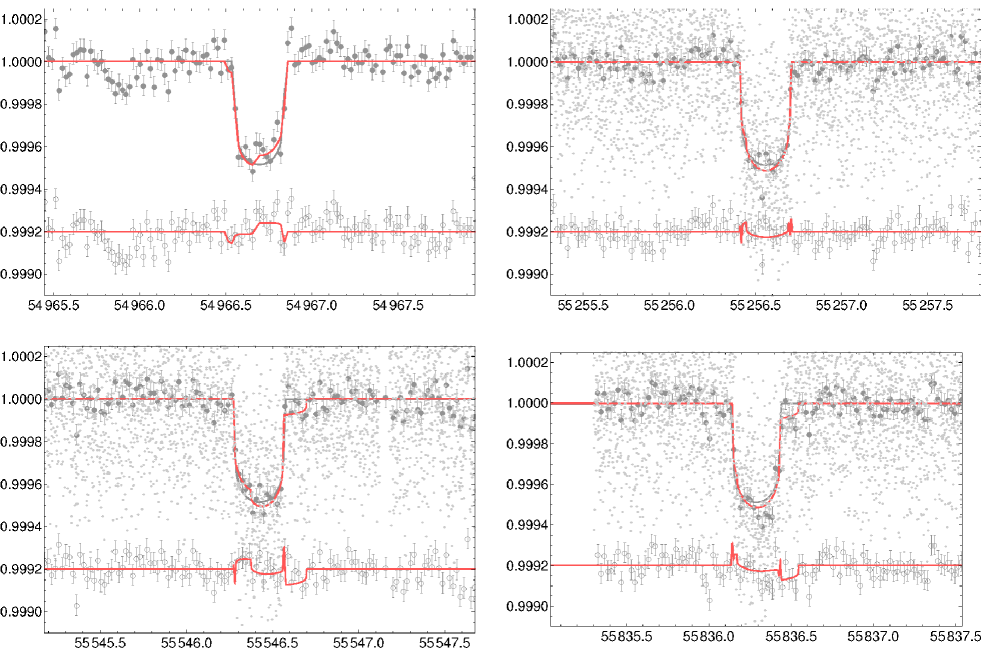
For the planet-only models, denoted by $\mathcal{P}_{i}$, we tried four models in total by exploring informative versus uninformative (free) priors on the limb darkening coefficients and circular versus eccentric priors on the orbit. The Bayesian evidences of the four models (see Table 5) are broadly similar with the biggest $\Delta\log\mathcal{Z}$ occurring between $\mathcal{P}_{\mathrm{LD-free},e_{B*}}$ and $\mathcal{P}_{\mathrm{LD-free}}$ where the former is favored at 1.2 $\sigma$. This marginal and insignificant difference suggests that the light curve contains insufficient information to distinguish between these scenarios. We consider that the null-hypothesis of a circular orbit is not over-turned by these results and we show the maximum a-posteriori light curve fit from model $\mathcal{P}_{\mathrm{LD-free}}$ in Figure 10.

The close proximity in evidence between the four planet-only models also highlights the benefits of Bayesian model averaging (BMA), as discussed earlier in §3.10. In Table 6, columns two shows the marginalzied parameters from model $\mathcal{P}_{\mathrm{LD-free},e_{B*}}$ alone and column three shows the effect of applying BMA over the four attempted planet-only models ($<\mathcal{P}_{k}>$).

4.2. Transit Timing and Duration Variations (TTVs & TDVs)

In addition to the four planet-only fits discussed in the previous subsection, we also tried three additional models designed to investigate the possibility of dynamical timing variations. These fits seek to determine the transit times and durations purely from the photometry and so we do not include the radial velocity data in this fit, which theoretically adds some extra information on the period and epoch of the transits. Since the input data is different, we require a new null hypothesis fit for which we can compare subsequent dynamical fits. To this end, we first tried a simple static transit model, $\mathcal{P}^{\prime}_{\mathrm{static}}$, where the dash is used to denote that this is a different family of model classes to those tried earlier (and not directly comparable).

$\mathcal{P}^{\prime}_{\mathrm{static}}$ is identical to the $\mathcal{P}_{\mathrm{LD-prior}}$ model fit except the radial velocity data is not included and so $K$ and $s$ are not free parameters in the fit. Next, we try model $\mathcal{P}^{\prime}_{\mathrm{TTV}}$, which allows each transit epoch to have a unique transit time parameter. The period of such a fit is unconstrained but does affect the estimate of $a_{B*}/R_{*}$ since this term is a function of $P_{B*}$ and $\rho_{*}$. Therefore, we apply a Gaussian prior on this term using the posterior distribution of $P_{B*}$ from model $\mathcal{P}^{\prime}_{\mathrm{static}}$. Finally, we try model $\mathcal{P}^{\prime}_{\mathrm{TTV+TDV}}$ in which each transit has entirely unique transit parameters.

After executing the fits in MultiNest, we find that a static model is strongly favored over the competing hypothesis (see Table 3). This is supported by a simple analysis of the derived TTVs and TDVs, as shown in Figure 3, which displays a lack of any significant deviations in either metric. We provide our derived transit times and durations in Table 4.

Table 3 Bayesian evidences of the three different models attempted to investigate the possibility of dynamical variations in the transits of Kepler-22b. A static orbit model is strongly favored over the competing hypotheses.

Model	$\log\mathcal{Z}$	Odds Ratio	$\sigma$ Confidence
$\mathcal{P}^{\prime}_{\mathrm{static}}$	$176873.289\pm 0.075$	1	-
$\mathcal{P}^{\prime}_{\mathrm{TTV}}$	$176864.058\pm 0.089$	$9.8\times 10^{-5}$	$-3.90$
$\mathcal{P}^{\prime}_{\mathrm{TTV+TDV}}$	$176847.848\pm 0.120$	$8.9\times 10^{-12}$	$-6.82$

Figure 3.— Left panel: TTVs measured for Kepler-22b, relative to the maximum a-posteriori ephemeris derived by model $\mathcal{P}^{\prime}_{\mathrm{static}}$. Squares represent the results determined by fitting each transit individually. Circles (slightly offset in transit epoch for clarity) represent the results determined by fitting global transit parameters but unique transit times. The agreement in both accuracy and precision is excellent. Right panel: TDVs determined by the individual transit fitting model (it is not possible to provide TDVs when assuming global transit shape parameters). Durations defined using the $\tilde{T}$ definition and TDVs computed relative to the maximum a-posteriori duration from model $\mathcal{P}^{\prime}_{\mathrm{static}}$.

Table 4 Transit times and durations derived for Kepler-22b. The transit timing and duration variations, derived from these values, are shown in Figure 3. These variations are computed relative the maximum a-posteriori metrics from the static model $\mathcal{P}^{\prime}_{\mathrm{static}}$; specifically $\tau_{0}=2455546.4246$ BJD_UTC, $P_{B*}=289.8645$ days and $\tilde{T}=419.4$ mins.

Epoch	$\tau_{i}$ [BJDUTC] from $\mathcal{P}^{\prime}_{\mathrm{TTV}}$	$\tau_{i}$ [BJDUTC] from $\mathcal{P}^{\prime}_{\mathrm{TTV+TDV}}$	$\tilde{T}$ [mins] from $\mathcal{P}^{\prime}_{\mathrm{TTV+TDV}}$
-2	$2454966.6969_{-0.0021}^{+0.0021}$	$2454966.6958_{-0.0026}^{+0.0025}$	$434.9_{-8.4}^{+8.6}$
-1	$2455256.5602_{-0.0020}^{+0.0020}$	$2455256.5603_{-0.0021}^{+0.0020}$	$418.7_{-7.2}^{+6.8}$
0	$2455546.4226_{-0.0020}^{+0.0019}$	$2455546.4226_{-0.0019}^{+0.0020}$	$412.2_{-6.2}^{+6.1}$
+1	$2455836.2910_{-0.0020}^{+0.0021}$	$2455836.2915_{-0.0019}^{+0.0019}$	$414.3_{-6.1}^{+6.0}$

4.3. Constraints on the Orbital Eccentricity

Leveraging both single-body asterodensity profiling (SAP) (Kipping et al., 2012a) and the radial velocities, we were able to allow for free eccentricity in the light curve fits. For simplicity, we used a uniform prior in $e_{B*}$ and $\omega_{B*}$ and discuss here the results from the model averaged planet-only posteriors (column heading $<\mathcal{P}_{k}>$ of Table 6). The $\Psi$ parameter (see Equation 6 of Kipping et al. 2012a), which is a single measure of the eccentricity as determined using SAP (Kipping et al., 2012a), is consistent with a circular orbit ($\Psi=1$) at $\Psi=1.4_{-0.6}^{+3.0}$. Further, the model averaged eccentricity is consistent with a circular orbit at $e_{B*}=0.13_{-0.13}^{+0.36}$ yielding a 95% confidence upper limit of $e_{B*}<0.71$.

4.4. Constraints on the Mass and Surface Gravity

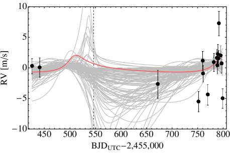
Our model averaged posteriors also reveal a lower stellar jitter than the 3 m s^-1 fixed assumption of B12, since we determine $s=2.4_{-0.6}^{+0.8}$ m s^-1. Combining the SAP constrained eccentricity, the lower stellar jitter and an overall more refined ephemeris than B12 (thanks to the extra transit included in this work) we derive a tighter constraint on the radial velocity semi-amplitude of $K=1.6_{-1.1}^{+2.2}$ m s^-1 compared to the B12 value of $K=4.9_{-7.4}^{+6.7}$ m s^-1. Our upper limit on this term, at 95% confidence, is $K<6.5$ m s^-1. Figure 4 shows the maximum likelihood radial velocity model for a circular orbit model.

Figure 4.— Radial velocities (black points) of Kepler-22b observed by B12. We overlay the maximum a-posteriori realization for an eccentric orbit planet (model $\mathcal{P}_{\mathrm{LD-free},e_{B*}}$) in red and one-hundred random draws from the joint posterior distribution in gray, which illustrate the uncertainty in the fit. The dashed vertical line marks the time of Q7 transit. The marginalized posterior for $K$, including Bayesian model averaging all over planet-only models, yields $K=1.6_{-1.1}^{+2.2}$ m s^-1.

Southworth et al. (2007) show how the surface gravity of an exoplanet can be computed from the transit and RV observables without requiring any assumption on the stellar/planet physical parameters. Exploiting this trick here, we find $g_{P}=26_{-19}^{+37}$ m s^-2. Thus, the surface gravity on Kepler-22b is most likely greater than that of the Earth but not dramatically so.

Our tighter constraint on $K$ can also be used to derive new constraints on the planet mass (assuming no moon is present). In order to do so, we require a stellar mass which we take from the asteroseismology analysis presented in B12 who found $0.970\pm 0.060$ $M_{\odot}$. Assuming this is distributed normally, our model averaged posteriors yield $M_{P}=6.9_{-6.2}^{+20.9}$ $M_{\oplus}$. For comparison, B12 quote three sets of upper limits for mass at $<36$ $M_{\oplus}$, $<82$ $M_{\oplus}$ and $<124$ $M_{\oplus}$ at a confidence of 1 $\sigma$, 2 $\sigma$ and 3 $\sigma$ respectively. At the same confidence levels, we estimate $<15$ $M_{\oplus}$, $<55$ $M_{\oplus}$ and $<148$ $M_{\oplus}$ demonstrating the generally much tighter constraint derived here.

4.5. Constraints on the Radius, Composition & Atmosphere

We may also use the stellar radius derived in B12 from asteroseismology, $R_{*}=0.979\pm 0.020$, to derive the physical planetary radius. Our model averaged posteriors yield $R_{P}=2.396_{-0.181}^{+0.088}$ $R_{\oplus}$ which is consistent with the $2.38\pm 0.13$ $R_{\oplus}$ value from B12. Note that two of the four models over which we have applied the Bayesian model averaging used free limb darkening coefficients and so are quite robust.

Following the method described in Kipping et al. (2013), one may compute the minimum atmospheric height ($R_{\mathrm{MAH}}$) for an exoplanet when the mass and radius are known, by employing a mass-radius relation for a water dominated planet. Using the mass-radius models of Zeng & Sasselov (2013), we compute $R_{\mathrm{MAH}}$ against the 75%-water-25%-silicate mass-radius contour to derive $R_{\mathrm{MAH}}=0.11_{-0.87}^{+1.04}$ $R_{\oplus}$ with 54% confidence of an atmosphere being present. Kepler-22b is therefore consistent with either a pure-water planet with a dense, low atmosphere or a rocky planet with a light, extended atmosphere. If Kepler-22b is cloudless, one should expect significant differences in the transmission spectroscopy signal between these two hypotheses. Thus, the true composition of Kepler-22b could be determined from transmission spectroscopy rather than a better mass estimate (although the latter would clearly work too).

Could the atmosphere of Kepler-22b be observable though? One may estimate the scale height of the planet’s atmosphere using the expression:

$$H =\frac{k_{B}T_{\mathrm{eq}}}{\mu g_{P}},$$ (12)

where $k_{B}$ is the Boltzmann constant, $T_{\mathrm{eq}}$ is the equilibrium temperature of the planet and $\mu$ is the mean molecular weight. The planet’s equilibrium temperature depends upon unknown quantities such as the albedo, emissivity and greenhouse effect but ignoring these complexities one may estimate $T_{\mathrm{eq}}=287.7_{-3.3}^{+8.4}$ K using the simple expression:

$$T_{\mathrm{eq}} =T_{*,\mathrm{eff}}\sqrt{\frac{1}{2(a_{B*}/R_{*})(1-e_{B*}^{2})^{1/4}}}.$$ (13)

If Kepler-22b is rocky with a light atmosphere, then we expect $\mu\sim 2$ which leads to $(H/R_{P})_{\mathrm{rocky}}=(3.0_{-1.7}^{+7.0})\times 10^{-3}$. If Kepler-22b is oceanic with a denser atmosphere, then one may adopt an Earth-like $\mu$ of $\mu\sim 28$ giving $(H/R_{P})_{\mathrm{oceanic}}=(0.22_{-0.13}^{+0.56})\times 10^{-3}$. Translating these into transit depths, we find a rocky planet has an atmospheric signal (using Eqn 36 of Winn 2010) of $\Delta\delta\sim 3.0_{-1.8}^{+7.9}$ ppm whereas an oceanic world has $\Delta\delta\sim 0.2_{-0.1}^{+0.6}$ ppm. We estimate that it is unlikely that these two scenarios could be distinguished with current instrumentation.

4.6. Constraints on Kepler-22b’s Insolation

Kepler-22b was originally claimed by B12 to lie within the habitable-zone of its host star. This statement in fact gave rise to Kepler-22b’s selection as a high-priority candidate for an exomoon investigation by the HEK project. Using our revised parameters and a recently revised definition of the habitable-zone (HZ) from Kopparapu et al. (2013), we may re-visit this important issue. This investigation will purely focus on whether the insolation received by Kepler-22b places the planet with the habitable-zone, as defined by Kopparapu et al. (2013), and will not address other factors affecting habitability such as the atmospheric composition.

Using the B12 “best-fit” parameters, Kopparapu et al. (2013) estimate Kepler-22b to lie slightly closer to its parent star than the inner-edge of the habitable zone, using the moist greenhouse limited model. However, in reality the uncertainties on the stellar and planetary parameters can be important, especially when an object lies very close to a boundary such as Kepler-22b. We may account for this by drawing a realization from our model averaged posteriors and testing whether that particular realization is consistent with a habitable planet or not. By simply counting the number of HZ realizations, one may phrase the question of habitability in a more statistically robust light.

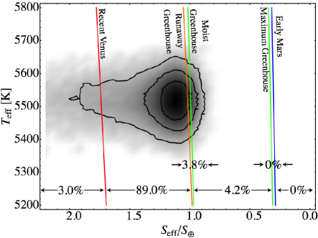
Using the revised habitable-zone (HZ) calculations from Kopparapu et al. (2013), we calculated the number of posterior samples, from the model averaged posterior, which could be classified as either “cold”, “warm” or “hot”. We use the maximum-greenhouse case as the outer-edge of the HZ and the moist-greenhouse case as the inner-edge. We note that this is the “conservative” habitable-zone since it is based on cloudless models and even the Earth falls on the inner-edge boundary for this model. The effective temperature and luminosity of the host star were assumed to have normal distributions with means and standard deviations given by the values quoted in B12.

We find that 95.8% of trials were “hot” and thus too close to the star to be habitable, with the remaining 4.2% being classed as warm (and thus habitable) and 0% cold. The so-called “empirical” HZ is defined as the recent-Venus and early-Mars limits leading to a wider HZ. Using these definitions, we find that 97.0% of trials are in the habitable-zone with the remaining 3.0% of trials being too hot. In Figure 5 we visualize these constraints and probabilities to provide a more statistical interpretation of an exoplanet’s habitability.

We therefore conclude that Kepler-22b has a $>95$% probability of being within the empirical HZ but $<5$% probability of being the conservative HZ, as defined by Kopparapu et al. (2013). We calculate that Kepler-22b receives only $13.7_{-8.7}^{+14.6}$% more insolation than the Earth, as the top of its atmosphere. We therefore consider that Kepler-22b can still be considered a good candidate for being within the habitable-zone, particularly if one considers models including clouds. We point out that even with an albedo of unity, the occultations of Kepler-22b would be undetectable with $\delta_{\mathrm{occ}}\simeq 14$ parts-per-billion.

Figure 5.— Joint posterior probability distribution of the stellar effective temperature ($T_{\mathrm{eff}}$) and the insolation received by Kepler-22b relative to that received by the Earth ($S_{\mathrm{eff}}/S_{\oplus}$). We overlay the various habitable-zone boundaries derived by Kopparapu et al. (2013) and the fraction of trials falling between the contours. Kepler-22b is likely warmer than the Earth but does fall within the empirical habitable-zone boundaries. Posteriors derived by Bayesian model averaging of all of the planet-only fits.

Table 5 Bayesian evidences of the ten different models (descriptions available in Table 2) attempted to explain the transit light curves of Kepler-22b. $\mathcal{P}$ models are those of a planet-only whereas $\mathcal{S}$ models are those of a planet-with-moon. Odds ratios computed relative to the strongrest planet-only model. $\sigma$ confidence column is computed relative to the best planet-only model ($\mathcal{P}_{\mathrm{LD-free},e_{P}}$).

Model	$\log\mathcal{Z}$	Odds Ratio	$\sigma$ Confidence
$\mathcal{P}_{\mathrm{LD-prior}}$	$176828.044\pm 0.058$	0.36	$-0.91$
$\mathcal{P}_{\mathrm{LD-prior},e_{B*}}$	$176828.797\pm 0.057$	0.77	$-0.29$
$\mathcal{P}_{\mathrm{LD-free}}$	$176827.602\pm 0.059$	0.23	$-1.19$
$\mathcal{P}_{\mathrm{LD-free},e_{B*}}$	$176829.054\pm 0.058$	1	-
$\mathcal{S}_{\mathrm{LD-prior}}$	$176831.704\pm 0.068$	14.15	1.81
$\mathcal{S}_{\mathrm{LD-prior},e_{B*}}$	$176832.491\pm 0.068$	31.09	2.14
$\mathcal{S}_{\mathrm{LD-prior},e_{SB}}$	$176841.248\pm 0.078$	197,599.99	4.56
$\mathcal{S}_{\mathrm{LD-free}}$	$176831.734\pm 0.069$	14.59	1.82
$\mathcal{S}_{\mathrm{LD-free},e_{B*}}$	$176832.979\pm 0.070$	50.65	2.33
$\mathcal{S}_{\mathrm{LD-free},e_{SB}}$	$176841.663\pm 0.078$	299,239.64	4.65

Table 6 Marginalized parameters of Kepler-22b after performing Bayesian model averaging. We show the results from four different ways of model averaging (descriptions available in Table 2). Bold-highlighted values represent our suggested final results. Parameters with a “max” subscript denote the 95% upper quantile. ^‡ = Computed using radial velocities and $M_{*}$ value from B12. ^† = Computed using $(M_{S}/M_{P})$ ratio derived purely from moon model combined with $M_{P}$ value derived from radial velocity and $M_{*}$ value from B12. ^× = Unphysically dense solutions were eliminated in computing this term, based upon maximum collisional stripping model from Marcus et al. (2010). ^∗ = Computed using $(M_{P}/M_{*})$ from moon dynamics and $M_{*}$ value from B12. ^⋄ = Computed purely from moon dynamics.

Parameter	$\mathcal{P}_{\mathrm{LD-free},e_{B*}}$	$\mathbf{<\mathcal{P}_{k}>}$	$<\mathcal{P}_{k},\mathcal{S}_{k}>$ for $e_{SB}=0$	$<\mathcal{P}_{k},\mathcal{S}_{k}>$
Planet’s transit parameters
$P_{B*}$ [days]	$289.86438_{-0.00080}^{+0.00084}$	$\mathbf{289.86444_{-0.00089}^{+0.0092}}$	$289.8654_{-0.0013}^{+0.0014}$	$289.8650_{-0.0011}^{+0.0012}$
$\tau_{0}$ [BJD${}_{\mathrm{UTC}}-2,455,000$]	$546.42471_{-0.00096}^{+0.00102}$	$\mathbf{546.4248_{-0.0011}^{+0.0011}}$	$546.4258_{-0.0015}^{+0.0016}$	$546.4238_{-0.0012}^{+0.0012}$
$(R_{P}/R_{*})$	$0.0219_{-0.0017}^{+0.0010}$	$\mathbf{0.02254_{-0.00187}^{+0.00054}}$	$0.02172_{-0.00110}^{+0.00079}$	$0.02249_{-0.00040}^{+0.00032}$
$(a_{B*}/R_{*})$	$186.4_{-1.2}^{+1.2}$	$\mathbf{186.4_{-1.2}^{+1.2}}$	$186.4_{-1.2}^{+1.2}$	$186.4_{-1.1}^{+1.1}$
$b_{B*}$	$0.756_{-0.516}^{+0.081}$	$\mathbf{0.805_{-0.328}^{+0.020}}$	$0.786_{-0.156}^{+0.031}$	$0.8116_{-0.0050}^{+0.0052}$
$i_{B*}$ [∘]	$89.749_{-0.026}^{+0.095}$	$\mathbf{89.750_{-0.015}^{+0.016}}$	$89.7455_{-0.0156}^{+0.0076}$	$89.7505_{-0.0027}^{+0.0027}$
$\tilde{T}$ [hours]	$6.953_{-0.089}^{+0.100}$	$\mathbf{6.972_{-0.080}^{+0.072}}$	$6.937_{-0.080}^{+0.078}$	$6.943_{-0.077}^{+0.069}$
$T_{14}$ [hours]	$7.30_{-0.14}^{+0.14}$	$\mathbf{7.38_{-0.17}^{+0.10}}$	$7.30_{-0.13}^{+0.11}$	$7.391_{-0.074}^{+0.065}$
$T_{23}$ [hours]	$6.59_{-0.25}^{+0.29}$	$\mathbf{6.53_{-0.14}^{+0.27}}$	$6.55_{-0.14}^{+0.17}$	$6.475_{-0.084}^{+0.074}$
$u_{1}$	$0.55_{-0.23}^{+0.25}$	$\mathbf{0.461_{-0.026}^{+0.241}}$	$0.461_{-0.052}^{+0.241}$	$0.467_{-0.026}^{+0.343}$
$u_{2}$	$0.10_{-0.33}^{+0.31}$	$\mathbf{0.231_{-0.339}^{+0.018}}$	$0.225_{-0.390}^{+0.019}$	$0.175_{-0.419}^{+0.065}$
$K$ [m s-1]	$1.8_{-1.2}^{+2.7}$	$\mathbf{1.6_{-1.1}^{+2.2}}$	$1.6_{-1.1}^{+2.0}$	$1.39_{-0.95}^{+1.66}$
$s$ [m s-1]	$2.36_{-0.59}^{+0.71}$	$\mathbf{2.41_{-0.63}^{+0.77}}$	$2.38_{-0.64}^{+0.77}$	$2.42_{-0.60}^{+0.74}$
$g_{P}$ [m s-2]	$29_{-20}^{+45}$	$\mathbf{26_{-19}^{+37}}$	$29_{-21}^{+37}$	$24_{-17}^{+29}$
$e_{B*}\sin\omega_{B*}$	$0.03_{-0.15}^{+0.31}$	$\mathbf{0.000_{-0.068}^{+0.215}}$	$0.049_{-0.049}^{+0.204}$	$0.00_{-0.00}^{+0.00}$
$e_{B*}\cos\omega_{B*}$	$0.08_{-0.27}^{+0.45}$	$\mathbf{0.00_{-0.12}^{+0.25}}$	$0.000_{-0.096}^{+0.138}$	$0.00_{-0.00}^{+0.00}$
$\Psi$	$1.41_{-0.57}^{+2.98}$	$\mathbf{1.00_{-0.10}^{+2.29}}$	$1.19_{-0.19}^{+1.15}$	$1.00_{-0.00}^{+0.00}$
Planet’s physical parameters
$R_{P}$ [$R_{\oplus}$]	$2.32_{-0.17}^{+0.13}$	$\mathbf{2.396_{-0.181}^{+0.088}}$	$2.31_{-0.12}^{+0.10}$	$2.399_{-0.062}^{+0.064}$
$M_{P}^{{\ddagger}}$ [$M_{\oplus}$]	$7.8_{-6.9}^{+22.0}$	$\mathbf{6.9_{-6.2}^{+20.9}}$	$7.2_{-6.4}^{+20.1}$	$6.6_{-5.9}^{+18.1}$
$M_{P,\mathrm{max}}^{{\ddagger}}$ [$M_{\oplus}$]	$<61.1$	$\mathbf{<52.8}$	$<48.9$	$<43.8$
$\rho_{P}^{{\ddagger}}$ [g cm-3]	$2.9_{-2.6}^{+8.8}$	$\mathbf{2.4_{-2.2}^{+7.5}}$	$3.2_{-2.9}^{+9.1}$	$2.6_{-2.3}^{+7.2}$
$\rho_{P,\mathrm{max}}^{{\ddagger}}$ [g cm-3]	$<25.4$	$\mathbf{<19.5}$	$<22.8$	$<17.4$
$R_{P,\mathrm{MAH}}^{{\ddagger}}$ [$R_{\oplus}$]	$0.00_{-0.88}^{+1.06}$	$\mathbf{0.11_{-0.87}^{+1.04}}$	$0.02_{-0.83}^{+1.04}$	$0.16_{-0.80}^{+1.02}$
$\mathrm{P}(R_{P,\mathrm{MAH}}>0)^{{\ddagger}}$	$0.50$	$\mathbf{0.54}$	$0.51$	$0.57$
$S_{\mathrm{eff}}$ $[S_{\oplus}]$	$1.19_{-0.12}^{+0.25}$	$\mathbf{1.137_{-0.087}^{+0.146}}$	$1.123_{-0.079}^{+0.088}$	$1.098_{-0.071}^{+0.074}$
$a_{B*}$ [AU]	$0.848_{-0.018}^{+0.018}$	$\mathbf{0.848_{-0.018}^{+0.018}}$	$0.848_{-0.018}^{+0.018}$	$0.848_{-0.018}^{+0.018}$
Satellite’s transit parameters
$P_{SB}$ [days]	-	-	$23_{-13}^{+33}$	$40_{-12}^{+21}$
$\phi_{SB}$ [∘]	-	-	$180_{-110}^{+120}$	$230_{-210}^{+110}$
$(a_{SP}/R_{P})$	-	-	$38_{-10}^{+14}$	$99_{-11}^{+19}$
$\rho_{S}$ [g cm-3]	-	-	$1.3_{-1.2}^{+6.4}$	$0.79_{-0.55}^{+1.24}$
$i_{SB}$ [∘]	-	-	$180_{-120}^{+120}$	$237_{-155}^{+47}$
$\Omega_{SB}$ [∘]	-	-	$-10_{-130}^{+140}$	$-35_{-24}^{+170}$
$(R_{S}/R_{P})$	$0$	$\mathbf{0}$	$0.320_{-0.047}^{+0.047}$	$0.341_{-0.026}^{+0.027}$
$(M_{S}/M_{P})$	$0$	$\mathbf{0}$	$0.023_{-0.015}^{+0.022}$	$0.0029_{-0.0020}^{+0.0030}$
$(M_{S}/M_{P})_{\mathrm{max}}$	-	-	$\mathbf{<0.062}$	$<0.0083$
Satellite’s physical parameters
$M_{S}^{\dagger}$ [$M_{\oplus}$]	$0$	$\mathbf{0}$	$0.13_{-0.12}^{+0.58}$	$0.015_{-0.014}^{+0.064}$
$M_{S,\mathrm{max}}^{\dagger\times}$ [$M_{\oplus}$]	-	-	$\mathbf{<0.54}$	$<0.16$
$R_{S}$ [$R_{\oplus}$]	$0$	$\mathbf{0}$	$0.74_{-0.10}^{+0.10}$	$0.819_{-0.062}^{+0.064}$
$R_{S,\mathrm{MAH}}$ [$R_{\oplus}$]	-	-	$-0.06_{-0.49}^{+0.41}$	$0.41_{-0.27}^{+0.22}$
$\mathrm{P}(R_{S,\mathrm{MAH}}>0)$	-	-	$0.44$	$0.93$
$e_{SB}\sin\omega_{SB}$	-	-	0	$0.06_{-0.23}^{+0.18}$
$e_{SB}\cos\omega_{SB}$	-	-	0	$0.31_{-0.69}^{+0.22}$
Parameters derived from moon model
$\rho_{P}^{*}$ [g cm-3]	-	-	$2.1_{-1.7}^{+8.4}$	$12.2_{-5.6}^{+8.4}$
$M_{P}^{*}$ [$M_{\oplus}$]	-	-	$4.6_{-3.8}^{+18.3}$	$31_{-14}^{+21}$
$M_{*}^{\diamond}$ [$M_{\odot}$]	-	-	$26_{-26}^{+8635}$	$0.095_{-0.093}^{+1.711}$
$R_{*}^{\diamond}$ [$R_{\odot}$]	-	-	$2.9_{-2.5}^{+17.3}$	$0.43_{-0.30}^{+0.71}$

5. INJECTED MOON RETRIEVAL

5.1. Generating Synthetic Moon Data

Before we discuss the results of our search for an exomoon around Kepler-22b  we first demonstrate the sensitivity limits achievable with this data set by injecting a synthetic moon signal into the data. In preparing this investigation, we wanted to realistically mimic the exact noise properties of the observed data i.e. we wish to reproduce all time-correlated noise features. We here describe several simple steps which enable us to accomplish this.

First, we proceed under the assumption that the real Kepler data does not show evidence for an exomoon (which is in fact our conclusion later in the paper). We then take our favored model, $\mathcal{P}_{\mathrm{LD-free}}$, and compute the residuals relative to the maximum a-posteriori realization (shown in Fig. 10 along with the residuals). We then “flip” these residuals by simply multiplying the fluxes by $-1$. We then re-add these flipped residuals to the maximum a-posteriori realization of model $\mathcal{P}_{\mathrm{LD-free}}$ to create a synthetic (but highly realistic) planet-only data set, $\mathcal{D}_{P}^{\prime}$ (where the “P” stands for planet-only and the dash implies synthetic data). Finally, we repeat this last step but instead add the flipped residuals to a pre-determined planet-with-moon model, in order to create a synthetic planet-with-moon data set, $\mathcal{D}_{S}^{\prime}$.

It’s important to stress that our technique is only capable of generating a single realization of synthetic data. However, it precisely reproduces the exact time-correlated structure of the real data with even the correct phasing relative to the transit events. Further, we make no assumptions about the nature of time-correlated noise or its origin, meaning this technique is a highly robust method for creating a synthetic data set.

The process of fitting for a planet-with-moon photodynamic signal using multimodal nested sampling as a computationally demanding one and so we limit ourselves to injecting a synthetic moon. For our synthetic moon, we choose a mass and radius equal to that of the Earth. The semi-major axis of the moon’s orbit is chosen such that it resides at the exact same relative distance within the Hill sphere that our Moon is separated from the Earth (25.7% of the Hill sphere). We choose to use a circular orbit moon and set the $\cos i_{SB}=\Omega_{SB}=\phi_{SB}=0$ for simplicity. The planet’s properties are set to that of the maximum a-posteriori values from model $\mathcal{P}_{\mathrm{LD-free}}$, except for the planet mass where we make the conservative choice of setting $M_{P}$ to the 95% upper quantile of $45.6$ $M_{\oplus}$ from the same model (this is conservative since it minimizes $M_{S}/M_{P}$ and thus any transit timing effects).

5.2. Fitting the Synthetic Moon Data

We first start by considering fitting the data $\mathcal{D}_{P}^{\prime}$, which does not contain a moon, but does include all of the time-correlated noise features seen in the real data. In fitting the data, for the sake of computational expediency, we only attempted two models - that of a circular-orbit planet ($\mathcal{P}$) and that of a circular-orbit planet with a circular-orbit moon ($\mathcal{S}$). We do not assume coplanarity in the moon fits and allow the limb darkening coefficients to be fitted for as was done in the real fits.

We find that a planet-only model is strongly favored at 5.0 $\sigma$ (see Table 7), as one should hope for given that no moon was injected. The 5.0 $\sigma$ preference also demonstrates the power of Bayesian model selection - the moon model uses more free parameters and thus is able to obtain higher likelihoods but the Bayesian evidence naturally penalizes the model for using these extra free parameters.

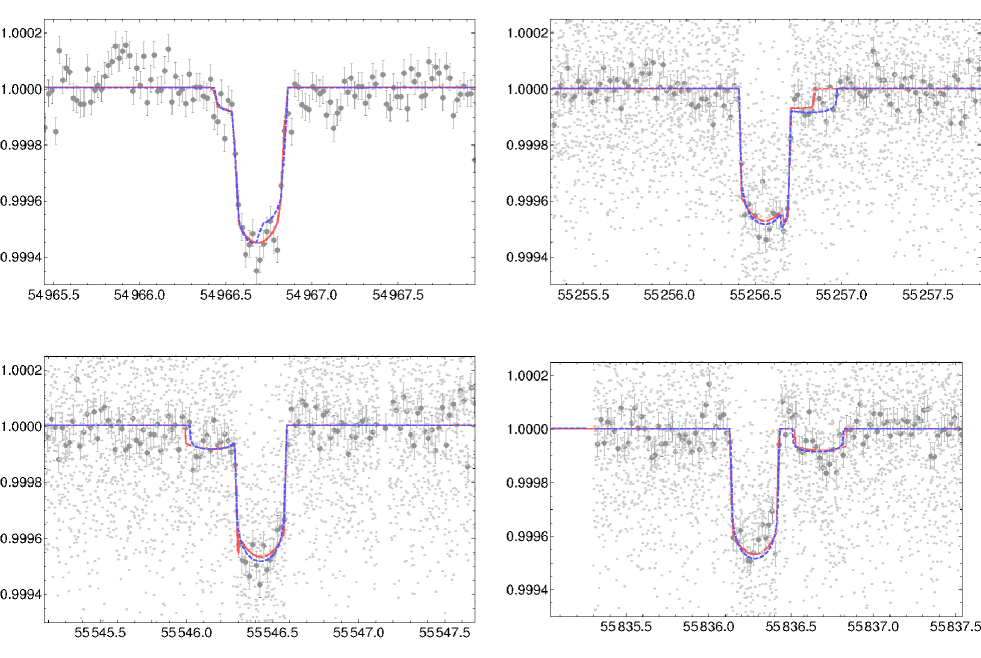
Focussing on the synthetic planet-with-moon data, $\mathcal{D}_{S}^{\prime}$, we find that the planet-with-moon is strongly favored at 8.3 $\sigma$ (see Table 7), again as expected. Whilst we only considered one realization for the orbital configuration of the moon, this very significant detection demonstrates that an Earth-like moon is readily detectable with the current data set. The accuracy of our blind retrieval of this injected moon can be visualized by comparing the light curves of the injected truth and the maximum a-posteriori blind recovery, as shown in Figure 6.

Table 7 Bayesian evidences two different models attempted to two different synthetic data sets of Kepler-22b. $\mathcal{D}_{P}^{\prime}$ is a synthetic planet-only model whereas $\mathcal{D}_{S}^{\prime}$ includes an injected Earth-like satellite. $\mathcal{P}$ models are those of a planet-only whereas $\mathcal{S}$ models are those of a planet-with-moon. Odds ratios and $\sigma$ confidences computed relative to the null-hypothesis of a planet-only.

Model	Data	$\log\mathcal{Z}$	Odds Ratio	$\sigma$ Confidence
$\mathcal{P}$	$\mathcal{D}_{P}^{\prime}$	$176872.912\pm 0.055$	1.00	-
$\mathcal{S}$	$\mathcal{D}_{P}^{\prime}$	$176858.767\pm 0.073$	$7.19\times 10^{-7}$	$-4.96$
$\mathcal{P}$	$\mathcal{D}_{S}^{\prime}$	$176802.104\pm 0.054$	1.00	-
$\mathcal{S}$	$\mathcal{D}_{S}^{\prime}$	$176838.801\pm 0.077$	$8.66\times 10^{+15}$	$+8.29$

Figure 6.— Injected moon fits. From left-to-right then top-to-bottom we show the chronological sequence of transits from synthetic data set $\mathcal{D}_{S}^{\prime}$ for Kepler-22b. Large dots are the LC-binned data and small dots are the SC data. The blue-dashed line shows the “truth”, which is Kepler-22b with an injected Earth-like moon. The red line shows the maximum a-posteriori planet-with-moon fit (i.e. a blind retrieval). We are able to recover the injected moon to a confidence of 8.3 $\sigma$. Animations of the transits are available at https://www.cfa.harvard.edu/$\sim$dkipping/kepler22.html

5.3. Habitability of the Injected Moon

As was done previously for Kepler-22b itself, we should now investigate whether the posterior distribution allows us to infer the habitability of our injected moon. Given the complex parameter degeneracies and low-to-moderate signal-to-noise of the injected moon signal, it is not immediately clear that we are able to definitively determine the moon’s habitability, given the broad and multimodal nature of the moon parameter posteriors.

This is further complicated by the fact that moons possess several extra sources and sinks of thermal energy compared to their host planets. If their orbit around the planet is elliptical, they can experience tidal heating, which can significantly affect surface temperatures even for small eccentricities (Reynolds et al., 1987; Scharf, 2006). They also suffer frequent stellar eclipses by their host planet, which can act as an effective energy sink (Heller, 2012). Both of these phenomena are extremely sensitive to the dynamical properties of the planet-moon pair. As recently demonstrated by Forgan & Kipping (2013) using latitudinal equilibrium balance models (LEBMs), even the orbital direction of the moon can have consequences for a telluric exomoon’s climate.

The habitable zone of an exomoon is therefore a non-trivial multi-parameter manifold, and it is not generally the case that if the host planet is partially or completely uninhabitable, the moon must be also. We therefore cannot rely on the habitable zone calculations of Kopparapu et al. (2013) (as was done for Kepler-22b) to determine the habitability of the exomoon. However, this does not preclude the possibility of a robust statistical analysis.

We employ the same LEBMs as described in Forgan & Kipping (2013) to investigate how well the posteriors allow us to recover the moon’s habitability. The LEBM allows us to evolve the moon’s surface temperature as a function of latitude assuming it is Earth-like in composition. In the simulation, the moon is subject to insolation from the host star, tidal heating from the host planet, eclipses by the planet, and infrared atmospheric cooling. The circulation of heat in the atmosphere is modeled by a diffusion equation (see also Williams & Kasting 1997 and Spiegel et al. 2008).

By using each realization of the posteriors as a set of inputs for a LEBM simulation, we can construct a distribution of exomoon climates, which can then be compared to the climate derived from the “true” injected parameters. Each LEBM simulation is classified in the following fashion (Forgan & Kipping, 2013):

1. Habitable Moons - these moons possess a habitable surface that covers at least 10% of the total area. This figure is time-averaged, and the standard deviation in habitable surface over this time is less than 10% of the mean.

2. Hot Moons - these moons display a surface habitability fraction of less than 10%, and typically possess surface temperatures above 373 K across all seasons, and are therefore conventionally uninhabitable.

3. Snowball Moons - these moons also display surface habitability of less than 10%, and have undergone a snowball transition to a state where the entire moon is frozen, and are therefore conventionally uninhabitable.

4. Variable Moons - these moons are similar to the habitable moons class above, but the standard deviation in habitable surface over time is high, greater than 10% of the mean.

The simulation run using the injected signal yields a stable, habitable climate with a mean temperature of approximately 320 K. The moon is on a close to circular orbit, and hence tidal heating does not play a significant role in the resulting climate. How does this compare to the data retrieved from the posteriors?

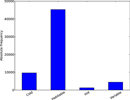
Figure 7 shows the resulting classification of all posteriors. Around 75% of all simulations run using the posterior data results in a habitable moon. The next most populous classification is the cold moon case - this is somewhat unsurprising, as the so-called “snowball” transition (generated by a rapid increase in albedo as surface water freezes) acts as a positive feedback mechanism, making cool climates colder, typically with no restorative warming mechanism to combat it. There is no analogous positive feedback at the other temperature extreme - indeed, hot climates possess a strong negative feedback mechanism through infrared cooling, and as a result the hot classification is less populated. As a further consequence of these differing feedback mechanisms, there is a small collection of moons which are classified as variable, the majority of which tend towards being too hot rather than too cold.

Figure 7.— The classification of the LEBM simulations carried out using the posterior parameter sets as input. We can see that the majority of the simulation runs identify the injected moon as “habitable” (i.e. at least 10% of its surface can sustain liquid water, and the standard deviation in this value is small). Around one sixth of the simulations are classified as too cold to be habitable, with around 2% of the simulations classifying the moon as too hot to be habitable.

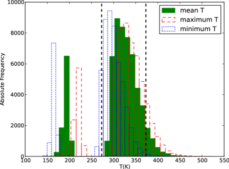
We can see this in more detail in Figure 8, which shows the minimum, maximum and mean temperatures exhibited by each simulation. The majority of simulations possess minima and maxima which fit inside the 100 K temperature range where water is expected to be liquid on a telluric planet’s surface. There is a small tail at $T>373$ K, but this is not as populous as the “snowball” population with mean temperatures around 200 K. The rapid albedo transition at 273 K ensures that few moons can maintain steady surface temperatures in this regime, giving rise to the gap centered on $T=250$ K. The mode of the mean temperature distribution is close to the “true” mean temperature of 320 K, with a long tail out to around 450 K.

Figure 8.— The minimum, maximum and mean temperatures of the LEBM simulations carried out using the posterior parameter sets as input. The vertical dashed lines indicate the freezing and boiling points of water at standard atmospheric pressure, $T=273$ K and $T=373$ K respectively.

In short, we can say with moderate confidence that we can reliably identify whether we expect a detected moon to be habitable or otherwise, given the posterior distribution, i.e. modeling the surface temperature using the posterior data gives similar results to those produced by modeling the injected signal. This being said, we should be cognizant of the long tail of the resulting temperature distributions produced, and we should also note that one in six posterior runs identify the moon as uninhabitable.

6. PLANET-WITH-MOON RESULTS

6.1. Circular Moon Fits

We first begin by discussing the fits attempted under the assumption that a putative exomoon follows a circular orbit around the planet Kepler-22b (although the planet itself is permitted to have an eccentric orbit). In total, there are four fits we attempted which fall into this category: a circular orbit planet with and without informative limb darkening priors (models $\mathcal{S}_{\mathrm{LD-prior}}$ and $\mathcal{S}_{\mathrm{LD-free}}$ respectively) and an eccentric orbit planet with and without informative limb darkening priors (models $\mathcal{S}_{\mathrm{LD-prior},e_{B*}}$ and $\mathcal{S}_{\mathrm{LD-free},e_{B*}}$ respectively).

None of these four fits show particularly significant model preferences, being in the range 1-2 $\sigma$ favorable over a simple planet-only fit (see Table 5). As with Kipping et al. (2013), we consider only models above $4$ $\sigma$ to be considered as candidate exomoons. Therefore, we find no compelling evidence for a circular orbit exomoon around Kepler-22b.

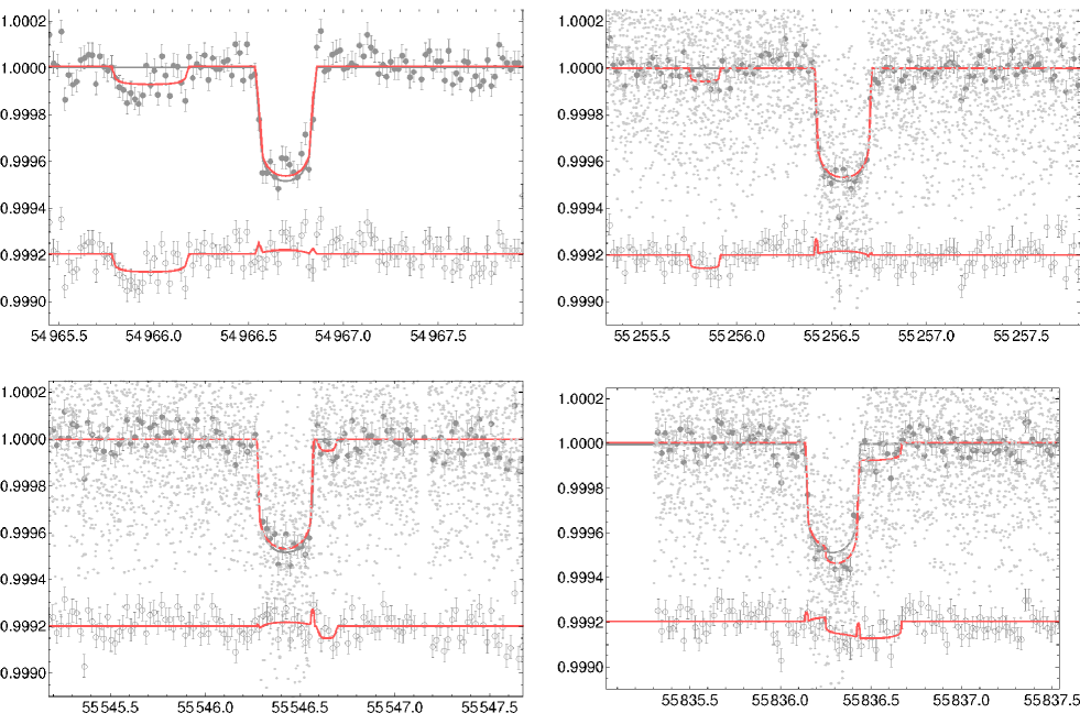
Out of the four models, $\mathcal{S}_{\mathrm{LD-free},e_{B*}}$ shows the highest significance at 2.3 $\sigma$ and we show the corresponding maximum a-posteriori light curve fit from this model in Figure 9, which has a $\Delta\chi^{2}=41.5$ better fit for $N=25971$ data points. Although the signal is not significant, we note that the solution corresponds to a moderately eccentric planet of $e_{B*}=0.29_{-0.15}^{+0.12}$ and mass $M_{P}=6.5_{-5.5}^{+20.4}$ $M_{\oplus}$ (derived purely from moon dynamical model, not from RVs), which is consistent with that derived from the RVs. The corresponding satellite would have a radius of $R_{S}=0.773_{-0.090}^{+0.083}$ $R_{\oplus}$ and mass of $M_{S}=0.23_{-0.20}^{+0.80}$ $M_{\oplus}$ with a broad density posterior spanning $\rho_{S}=2.9_{-2.5}^{+9.5}$ g cm^-3. We estimate that only 64.7% of trials yield a physically plausible density by using the internal structure models of Zeng & Sasselov (2013).

As with our previous survey (Kipping et al., 2013), despite finding a non-detection we derive upper limits on the mass-ratio for a putative exomoon. Applying Bayesian model averaging over the four planet-only models and the four circular-orbit moon models (i.e. eight models in total) allows us to compute a model-averaged posterior for the mass ratio of $(M_{S}/M_{P})=0.023_{-0.015}^{+0.022}$. The 95% upper quantile of this posterior gives $(M_{S}/M_{P})<0.062$ i.e. 6.2%. For the radius-ratio posterior, $(R_{S}/R_{P})$, we note that 97.8% of trials were positive (recall we explored negative radius solutions), corresponding to 2.0 $\sigma$ significance using the odds-ratio test given by Equation 4 in Kipping et al. (2010).

Unlike previous planets studied, we have a reliable mass constraint for the host planet from the radial velocities meaning we can translate this mass ratio into a physical mass upper limit. Further more, Kepler-22b is a validated small-radius planet and so must conform with physically plausible mass-radius constraints. We therefore generate a posterior for $M_{S}$ in absolute units and then eliminate any trials where either the joint posterior of $M_{P}$-$R_{P}$ or $M_{S}$-$R_{P}$ corresponds to a density exceeding the maximum mass stripping limit of an iron-rich planet derived by Marcus et al. (2010). We find that this eliminates  5% of the posterior trials. From this, we estimate that $M_{S}<0.54$ $M_{\oplus}$ to 95% confidence. We therefore conclude that Kepler-22b is highly unlikely to host an Earth-like moon on a circular orbit.

Figure 9.— Circular moon fits. From left-to-right then top-to-bottom we show the chronological sequence of transits observed by Kepler for Kepler-22b. Large dots are the LC-binned data and small dots are the SC data. The gray solid line shows the maximum a-posteriori planet-only fit with the corresponding residuals shown offset below. The red line shows the maximum a-posteriori planet-with-moon fit from model $\mathcal{S}_{\mathrm{LD-free},e_{B*}}$. In the residuals, we also show the difference between the two fitted models in red for comparison. Note that this line is not equal to the flux change which would be caused by the moon component in isolation, rather it is purely the difference between the maximum a-posteriori planet-only fit and the maximum a-posteriori planet-with-moon fit.

6.2. Eccentric Moon Fits

Both of the eccentric moon models, $\mathcal{S}_{\mathrm{LD-prior},e_{SB}}$ and $\mathcal{S}_{\mathrm{LD-free},e_{SB}}$, are strongly favored over the planet-only models at $>4$ $\sigma$ and thus are significant enough to be further considered as a candidate, with the latter model being slightly preferred. In a $\chi^{2}$ sense, the maximum a-posteriori realization from model $\mathcal{S}_{\mathrm{LD-free},e_{SB}}$ is superior to planet-only fit $\mathcal{P}_{\mathrm{LD-free},e_{B*}}$ at $\Delta\chi^{2}=79.8$ and the circular moon fit $\mathcal{S}_{\mathrm{LD-free}}$ at $\Delta\chi^{2}=38.3$.

The light curve fits appear to be heavily influenced by a transit-like feature occurring prior to the transit of Kepler-22b in the long-cadence data of Q1 (see Fig 10). Unlike the circular orbit fits, the eccentric fits have the flexibility to both explain this feature and yet remain comptable with the rest of the time series. Although our Bayesian model selection approach penalizes models for using more free parameters, such as these eccentric fits, our likelihood function assumes pure Gaussian noise and so we must remain cautious in interpreting what could simply be a time-correlated noise feature of unknown origin. This is particularly salient in light of the fact CoFiAM identified Q1 has having the greatest degree of autocorrelation out of the four transits used in this work (see §2.2).

One of the key tests described in Kipping et al. (2013) for vetting such systems is to inspect the derived posteriors and see if they are physically plausible or not. The Bayesian model averaged posteriors of all ten models attempted are dominated by the eccentric moon fits due to the large odds ratios and so we inspect these posteriors to vet these solutions. The dynamically derived planet density appears rather high at $\rho_{P}=12.2_{-5.6}^{+8.4}$ g cm^-3 yielding $M_{P}=31_{-14}^{+21}$ $M_{\oplus}$. This may be compared with the RV derived $M_{P}$ from the same posteriors of $M_{P}=6.5_{-5.8}^{+17.2}$ $M_{\oplus}$ and $M_{P}<40.4$ to 95% confidence, from which we conclude the result is slightly incompatible.

Before commenting on the putative exomoon’s composition, we note that the orbit appears excited with $e_{SB}=0.46_{-0.22}^{+0.12}$ and inclined $\sim 15^{\circ}$ (highly multimodal posterior) from the planet’s orbital plane. For the composition, we find an unusually low density of $\rho_{S}=0.79_{-0.55}^{+1.24}$ g cm^-3, which favors a bulk density below that of water/ice. Using the minimum atmospheric height method of Kipping et al. (2013) and using the derived moon radius of $R_{S}=0.818_{-0.062}^{+0.065}$ $R_{\oplus}$, we find that 93.3% of trials yield a radius exceeding a pure water/ice composition moon. The only way to explain this situation is an extended atmosphere but given that $M_{S}=0.015_{-0.013}^{+0.062}$ $M_{\oplus}$, the moon would rapidly lose an atmosphere, given the equilibrium temperature of $286\pm 3$ K. Given that Kepler-22 is not a young star (B12) and so presumably the exomoon has had plenty of time for an atmosphere to have escaped already, we must invoke a continuously replenishing atmosphere to explain these values.

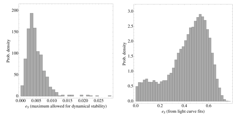
The orbit of the inclined, eccentric moon can also be shown to be unstable. The Hill stability of inclined low-mass binaries in the three body problem was explored extensively in Donnison (2010). Donnison (2010) presented expressions for the maximum stable eccentricity of an inclined binary in the case where the combined planet-moon mass is much less than that of the host star, as is applicable for the Kepler-22b system. Using Equation 25 of this work, which has a complex dependency with $M_{S}$, $M_{P}$, $M_{*}$, $i_{SB}$, $a_{B*}$ and $a_{SP}$, we estimate that 99.97% of the joint posterior realizations exhibit Hill instability (see Figure 11). Driving this determination is the wide-separation of the putative moon’s orbit of $a_{SP}\simeq 100$ $R_{P}$ combined with the inclined, eccentric nature of the orbit.

We therefore consider that the solution is a false-positive, likely induced by residual autocorrelation in the long-cadence data of Q1. This false transit signal can only be fitted by driving to high eccentricities. One effect of high exomoon eccentricity is to increase the r.m.s. TTV and TDV amplitudes induced by the moon on the planet (Kipping, 2009a). Since no TTVs or TDVs occur in the Kepler-22b data (Figure 3), the algorithm is forced to set the moon to be a very low-mass object in order to explain the full data set.

Figure 10.— Eccentric moon fits. From left-to-right then top-to-bottom we show the chronological sequence of transits observed by Kepler for Kepler-22b. Large dots are the LC-binned data and small dots are the SC data. The gray solid line shows the maximum a-posteriori planet-only fit with the corresponding residuals shown offset below. The red line shows the maximum a-posteriori planet-with-moon fit from model $\mathcal{S}_{\mathrm{LD-free},e_{SB}}$. In the residuals, we also show the difference between the two fitted models in red for comparison. Note that this line is not equal to the flux change which would be caused by the moon component in isolation, rather it is purely the difference between the maximum a-posteriori planet-only fit and the maximum a-posteriori planet-with-moon fit.

Figure 11.— Left: Using Equation 25 of Donnison (2010), we calculate the posterior distribution of the maximum allowed exomoon eccentricity for Hill stability. Right: Derived distribution of the light curve fitted exomoon eccentricity from the model averaged posteriors, for which 99.97% of trials are Hill unstable.

6.3. Excluded Moon Mass

It has been shown that the $>4$ $\sigma$ eccentric exomoon signal is a false positive i.e. spurious detection. Spurious detections cannot be used to derive upper limits for reasons discussed in Kipping et al. (2013) and so we do not use these results to derive our excluded moon mass limits presented here. This is equivalent to assigning a negligible prior model probability to models $\mathcal{S}_{\mathrm{LD-free},e_{SB}}$ and $\mathcal{S}_{\mathrm{LD-prior},e_{SB}}$. Performing Bayesian model averaging over the remaining eight models provides reliable upper limits on the presence of an exomoon. We find that $(M_{S}/M_{P})<6.2$% to 95% confidence which can be converted into a physical mass estimate by leveraging the $(M_{P}/M_{*})$ constraint from the radial velocities and $M_{*}$ from asteroseismology to give $M_{S}<0.54$ $M_{\oplus}$ to 95% confidence.

7. SUMMARY

Due to the large number of results in this paper, we summarize the most important findings below:

• We have conducted the first search for an exomoon around a habitable-zone exoplanet and find no compelling evidence for a companion to Kepler-22b. Furthermore, we constrain $M_{S}<0.54$ $M_{\oplus}$ to 95% confidence.

• We have demonstrated that an Earth-like moon would be detectable around Kepler-22b with the current data to 8.3 $\sigma$ by signal injection and recovery.

• We have further shown that such an injected moon would very likely have conditions suitable for liquid water on the surface through latitudinal energy balance modelling (LEBM) of the posteriors samplings.

• We have introduced several new improvements to the HEK methodology, including exploring negative-radius, retrograde and eccentric moon solutions, free limb darkening sampled from a Dirichlet prior and Bayesian model averaging.

• For the first time, the radial velocities of Kepler-22b have been fitted with a model accounting for free eccentricity and free stellar jitter. Combined with an updated ephemeris from a new transit in Q11, we derive a tighter mass constraint on Kepler-22b of $M_{P}<52.8$ $M_{\oplus}$ to 95% confidence.

• Utilizing Single-body Asterodensity Profiling (SAP) and the radial velocities, we provide the first constraints on the orbital eccentricity of Kepler-22b with $e_{B*}=0.13_{-0.13}^{+0.36}$ and $e_{B*}<0.71$ to 95% confidence.

• From our refined transit model, we estimate that Kepler-22b has a $>95$% probability of lying within the empirical habitable-zone but a $<5$% probability of lying within the conservative habitable-zone (as defined by Kopparapu et al. 2013). We derive an insolation of $S_{\mathrm{eff}}=1.137_{-0.087}^{+0.146}$ $S_{\oplus}$.

The above results were derived through photodynamical modeling and multimodal nested sampling regression requiring 49.7 years of CPU time⁹. Compared to other systems analyzed during the HEK project (Nesvorný et al., 2012; Kipping et al., 2013), this load is higher than average due to the high-resolution fitting mode employed here (see §3.9). Nevertheless, this highlights the unique computational challenges of seeking exomoons.

We find no evidence for an Earth-like exomoon around Kepler-22b and yet have shown that the present data can easily detect such an object via signal injection. Current observations therefore dictate that Kepler-22b does not possess an Earth-like habitable moon. Our results then, combined with the very robust measurement of the planet’s radius, mean that Kepler-22 does not possess an Earth analog. This does not mean that the system possesses no options for an inhabited world, with notable possiblities being a smaller, presently undetectable moon (e.g. $M_{S}\sim 0.2$ $M_{\oplus}$) or a possible ocean on Kepler-22b. However, it is now clear that this is not the location to find a second Earth.

To date, nine systems have been surveyed for exomoons by the HEK project (Nesvorný et al., 2012; Kipping et al., 2013) and no detections have been made with most cases yielding detection sensitivities of $\sim M_{\oplus}$. We caution that the number of systems analyzed remains too small to draw any meaningful conclusions about the occurrence of large moons, $\eta_{\leftmoon}$, but this is the ultimate goal of our project. In coming work, two future surveys will focus on i) M-dwarf host star planetary candidates and ii) planets exhibiting repeated visual anomalies. Slowly then, the landscape of the frequency of exomoons will be revealed.

References

- Anglada-Escudé et al. (2012) Anglada-Escudé, G. et al., 2012, ApJ, 751, L16
- Anglada-Escudé et al. (2013) Anglada-Escudé, G., Rojas-Ayala, b., Boss, A. P., Weinberger, A. J. & Lloyd, J. P., 2013, A&A, 551, 48
- Balan & Lahav (2009) Balan, S. T. & Lahav, O., 2009, MNRAS, 394, 1936
- Borucki et al. (2012) Borucki, W. J. et al., 2012, ApJ, 745, 120 (B12)
- Charbonneau et al. (2009) Charbonneau, D. et al., 2009, Nature, 462, 891
- Domingos et al. (2006) Domingos, R. C., Winter, O. C. & Yokoyama, T., 2006, MNRAS, 373, 1227
- Donnison (2010) Donnison, J. R., 2010, P&SS, 58, 1169
- Feroz et al. (2009a) Feroz, F., Hobson, M. P. & Bridges, M., 2009a, MNRAS, 398, 1601
- Feroz et al. (2009b) Feroz, F., Gair, J. R., Hobson, M. P. & Porter, E. K., 2009b, CQG, 26, 215003
- Forgan & Kipping (2013) Forgan, D. & Kipping, D. M., 2013, MNRAS, accepted (astro-ph:1304.4377)
- Gilliland et al. (2010) Gilliland., R. et al., 2010, ApJ, 713, 160
- Vladilo et al. (2013) Vladilo, G., Murante, G., Silva, L., Provenzale, A., Ferri, G. & Ragazzini, G., 2013, ApJ, 767, 65
- Heller (2012) Heller, R., 2012, A&A, 545, L8
- Heller & Barnes (2012) Heller, R. & Barnes, R., 2012, arXiv:1210.5172
- Heller & Barnes (2013) Heller, R. & Barnes, R., 2013, AsBio, 13, 18
- Kipping (2009a) Kipping, D. M., 2009, MNRAS, 392, 181
- Kipping (2009b) Kipping, D. M., 2009, MNRAS, 396, 1797
- Kipping et al. (2009) Kipping, D. M., Fossey, S. J. & Campanella, G., 2009, MNRAS, 400, 398
- Kipping (2010a) Kipping, D. M., 2010, MNRAS, 408, 1758
- Kipping et al. (2010) Kipping, D. M. et al., 2010, ApJ, 725, 2017
- Kipping & Bakos (2011a) Kipping, D. M. & Bakos, G. A., 2011, ApJ, 730, 50
- Kipping & Bakos (2011b) Kipping, D. M. & Bakos, G. A., 2011, ApJ, 733, 36
- Kipping (2011a) Kipping, D. M., 2011, MNRAS, 416, 689
- Kipping (2011b) Kipping, D. M., 2011, PhD thesis, University College London (astro-ph:1105.3189)
- Kipping et al. (2012a) Kipping, D. M., Dunn, W., Jasinksi, J. M. & Manthri, V. P., 2012, MNRAS, 421, 1166
- Kipping et al. (2012b) Kipping, D. M., Bakos, G. Á., Buchhave, L., Nesvorný, D. & Schmitt, A. 2012, ApJ, 750, 115
- Kipping et al. (2013) Kipping, D. M., Hartman, J., Buchhave, L., Schmitt, A., Bakos, G. Á. & Nesvorný, D., 2013, ApJ, 770, 101
- Kipping et al. (2013) Kipping, D. M., Spiegel, D. S., Sasselov, D., 2013, MNRAS, 434, 1883
- Kipping (2013) Kipping, D. M., 2013, MNRAS, accepted (astro-ph:1308.0009)
- Kopparapu et al. (2013) Kopparapu, R. K. et al., 2013, ApJ, 765, 131
- Kurucz (2006) Kurucz R., 2006, Stellar Model and Associated Spectra (http://kurucz.harvard.edu/grids.html)
- Mandel & Agol (2002) Mandel, K. & Agol, E., 2002, ApJ, 580, 171
- Marcus et al. (2010) Marcus, R. A., Sasselov, D., Hernquist, L. & Stewart, S. T. 2010, ApJ, 712, 73
- Mazeh et al. (2010) Mazeh, T. & Faigler, S., 2010, A&A, 521, 59
- Neubauer et al. (2012) Neubauer, D., Vrtala, A., Leitner, J. J., Gertrude F. M., Hitzenberger, R., 2012, P&SS, 73, 397
- Nesvorný et al. (2012) Nesvorný, D. Kipping, D. M., Buchhave, L. A., Bakos, G. A., Hartman, J. & Schmitt, A., 2012, Science, 336, 1133
- Parkinson & Liddle (2013) Parkinson, D. & Liddle, A. 2013, SAM, 6, 3
- Pal (2008) Pal, A., 2008, MNRAS, 390, 281
- Reynolds et al. (1987) Reynolds, R. T., McKay, C. P. & Kasting, J. F., 1987, AdSpR, 7, 125
- Scharf (2006) Scharf, C. A., 2006, ApJ, 648, 1196
- Spiegel et al. (2008) Spiegel, D. S., Menou, K. & Scharf, C. A., 2008, ApJ, 681, 1609
- Southworth et al. (2007) Southworth, J., Wheatley, P. J. & Sams, G., 2007, MNRAS, 379, 11
- Vogt et al. (2010) Vogt, S. S., Butler, R. P., Rivera, E. J., Haghighipour, N., Henry, G. W., Williamson, M. H. 2010, ApJ, 723, 954
- Waldmann (2012) Waldmann, I. P., Tinetti, G., Drossart, P., Swain, M. R., Deroo, P. & Griffith, C. A., 2012, ApJ, 744, 35
- Williams & Kasting (1997) Williams, D. M. & Kasting, J. F., 1997, Icarus, 129, 254
- Winn (2010) Winn, J. N. 2010, arXiv:1001.2010
- Zeng & Sasselov (2013) Zeng, L. & Sasselov, D., 2013, PASP, submitted (astro-ph:1301.0818)
- Zsom et al. (2013) Zsom, A., Seager, S. & de Wit, J., 2013, ApJ, submitted (astro-ph:1304.3714)