Evidence for temperature dependent spin-diffusion as a mechanism of intrinsic flux noise in SQUIDs

Abstract

The intrinsic flux noise observed in superconducting quantum interference devices (SQUIDs) is thought to be due to the fluctuation of electron spin impurities, but the frequency and temperature dependence observed in experiments do not agree with the usual $1/f$ models. We present theoretical calculations and experimental measurements of flux noise in rf-SQUID flux qubits that show how these observations, and previous reported measurements, can be interpreted in terms of a spin-diffusion constant that increases with temperature. We fit measurements of flux noise in sixteen devices, taken in the $20-80$ mK temperature range, to the spin-diffusion model. This allowed us to extract the spin-diffusion constant and its temperature dependence, suggesting that the spin system is close to a spin-glass phase transition.

I Introduction

Low frequency fluctuations of magnetic flux are a dominant noise source in a wide range of superconducting circuits, including SQUID-based magnetometers and rf-SQUID flux qubits used as the building blocks for quantum computing architectures.clarke08 In the case of qubits, this magnetic flux noise places fundamental limits on the performance and scalability of such architectures. Low frequency flux noise is widely thought to be due to fluctuations of magnetic impurities local to the superconductor wiringkoch07 ; bialczak07 ; sendelbach08 but the identity of these impurities and the physical mechanism producing the observed fluctuations is not known. Understanding the fundamental origin of flux noise is important not only to aid in its reduction in superconducting devices, but also may provide insight into the behavior of disordered ensembles of spins at low temperature. Indeed, flux noise experimentssendelbach08 suggested the presence of a spin-glass phase, motivating further computational studies of fluctuations in spin-glasses.chen10

Some likely candidates for spin impurities include dangling-bonds in the oxide surrounding the superconducting wire,desousa07 or disorder-induced localized states at the superconductor-insulator interface.choi09 The key point is that the spins must be located close to the superconducting wire for their flux to be significant. Any mechanism that produces spin dynamics will contribute to flux noise. Since spin-lattice relaxation is suppressed at low temperatures,desousa07 it was proposed that the RKKY interaction between spins is responsible for spin-diffusion and flux noise;faoro08 however their theory of spin-diffusion predicted $1/f$ noise independent of temperature, thus it does not explain the frequency and temperature dependence of flux noise observed in SQUIDs.wellstood87 ; anton13

Anton et al.anton13 recently presented a comprehensive experiment that seemed to contradict the spin-diffusion interpretation; they measured flux noise above $T=100$ mK and proposed a power law fit of the form $A^{2}/f^{\alpha}$, showing that the temperature dependence of $A$ and $\alpha$ leads to the presence of a pivot frequency, below (above) which the noise decreases (increases) with increasing temperature.

In this article, we propose a theory of spin-diffusion in SQUIDs that explains these observations. We predict the presence of a crossing band supported by Ref. anton13, and present additional experimental measurements of flux noise in superconducting flux qubits in a temperature range between 20 and 80 mK that confirm this prediction. The model allows us to use these measurements to estimate the spin-diffusion constant and explore its dependence on temperature.

II Flux produced by spins near SQUID wiring

We assume an ensemble of spin-$1/2$ impurities distributed nearby the SQUID wire; each spin is located at $\bm{R}_{i}$, and described by the dimensionless spin operator $\bm{s}_{i}$. The SQUID detects a total flux of

$$\Phi(t)=\sum_{i}\bm{F}(\bm{R}_{i})\cdot\bm{s}_{i}(t),$$ (1)

with a flux vector $\bm{F}(\bm{R}_{i})$ representing the dependence of the flux on different spin orientations.

We can find an explicit expression for $\bm{F}(\bm{R}_{i})$ by noting that the coupling energy between the spin and the SQUID is ${\cal H}_{\rm{s-SQ}}=-\bm{\mu}_{i}\cdot\bm{B}(\bm{R}_{i})$, where $\bm{\mu}_{i}=-g\mu_{B}\bm{s}_{i}$ is the magnetic moment of the electron spin, $g\approx 2$ is its $g$-factor, $\mu_{B}$ is the Bohr magneton, and

$$\bm{B}(\bm{R}_{i})=\frac{\mu_{0}}{4\pi}\int d^{3}r\frac{\left(\bm{r}-\bm{R}_{i}\right)\times\bm{J}_{\rm{SQUID}}(\bm{r})}{\left|\bm{r}-\bm{R}_{i}\right|^{3}}$$ (2)

is the magnetic field produced by the SQUID’s current density $\bm{J}_{\rm{SQUID}}(\bm{r})$. The flux-inductance theorem (proven in Section 5.17 of Ref. jackson99, ) implies that the flux produced by the spin must relate to the coupling energy according to $\Phi_{i}={\cal H}_{\rm{s-SQ}}/I_{\rm{SQUID}}$, where $I_{\rm{SQUID}}$ is the total current flowing through the SQUID’s loop. From this we get an explicit expression for $\bm{F}(\bm{R}_{i})$:

$$\bm{F}(\bm{R}_{i})=\frac{g\mu_{B}\mu_{0}}{4\pi}\int d^{3}r\frac{(\bm{r}-\bm{R}_{i})\times\bm{J}_{\rm{SQUID}}(\bm{r})}{\left|\bm{r}-\bm{R}_{i}\right|^{3}I_{\rm{SQUID}}}.$$ (3)

We performed explicit numerical calculations of Eq. (3) for the particular geometry of the devices we tested. We provide details on the geometry and the numerical calculations in Appendix A.

III Model of flux noise due to spin-diffusion

The thermal equilibrium flux noise

$$\tilde{S}_{\Phi}(f)=\int_{-\infty}^{\infty}dt\;\textrm{e}^{2\pi ift}\langle\Phi(t)\Phi(0)\rangle,$$ (4)

can be computed in the so called spin-diffusion regime, where only long wavelength fluctuations of the spin system are taken into account. This is done by considering a coarse-grained impurity spin field, $\bm{M}(\bm{r},t)=\sum_{i}\bm{s}_{i}\delta(\bm{r}-\bm{R}_{i})$, with the flux written as

$$\Phi(t) = \int d^{2}r\bm{F}(\bm{r})\cdot\bm{M}(\bm{r},t)$$ (5)

$$= \frac{1}{(2\pi)^{2}}\int d^{2}k\int df\textrm{e}^{-2\pi ift}\bm{\tilde{F}}^{*}(\bm{k})\cdot\bm{\tilde{M}}(\bm{k},f),$$

with $\bm{\tilde{F}}(\bm{k})=\int d^{2}r\;\textrm{e}^{-i\bm{k}\cdot\bm{r}}\bm{F}(\bm{r})$ and $\bm{\tilde{M}}(\bm{k},f)=\int d^{2}r\int dt\;\textrm{e}^{-i(\bm{k}\cdot\bm{r}-2\pi ft)}\bm{M}(\bm{r},t)$.

We consider a model Hamiltonian of exchange coupled spins,

$${\cal H}_{\rm{s-s}}=\sum_{i<j}J_{ij}\bm{s}_{i}\cdot\bm{s}_{j}.$$ (6)

In the paramagnetic phase (where $\langle\bm{s}_{i}\rangle=0$) the spin field will satisfy the following Langevin equation,chaikin00

$$\frac{\partial\bm{M}}{\partial t}=D\nabla^{2}\bm{M}+\bm{\zeta},$$ (7)

where $D$ is a diffusion constant (possibly temperature dependentbennet65 ), and $\bm{\zeta}$ is a random force that drives the spins into thermal equilibrium with themselves. This implies the following correlation for the random force,chaikin00

$$\left\langle\zeta_{\alpha}(\bm{r},t)\zeta_{\beta}(\bm{r}^{\prime},t^{\prime})\right\rangle=\frac{\sigma D}{2}\frac{\chi}{\chi_{0}}\nabla^{2}\delta(\bm{r}-\bm{r^{\prime}})\delta(t-t^{\prime})\delta_{\alpha\beta},$$ (8)

where $\sigma$ is the area density for spins, $\chi$ is the interacting spin susceptibility (defined as $\chi=\partial\langle M\rangle/\partial B$ at $B=0$), and $\chi_{0}=-g\mu_{B}\sigma/(4k_{B}T)$ is the free spin (Curie) susceptibility. This random force correlator is chosen so that the fluctuation-dissipation theorem is satisfied (thus leading to the expected thermal equilibrium state at long times). We emphasize that we assume the spins are decoupled from their lattice, so that the total magnetization $\sum_{i}\bm{s}_{i}$ is conserved [the presence of $\nabla^{2}$ in Eq. (8) ensures this conservation law].

Writing Eqs. (4)–(8) in Fourier space and evaluating the spin-spin correlation function leads to a convenient expression relating SQUID geometry to flux noise:

$$\tilde{S}_{\Phi}(f)=\frac{\sigma}{2(2\pi)^{4}}\frac{\chi}{\chi_{0}}\int d^{2}k|\tilde{\bm{F}}(\bm{k})|^{2}\frac{Dk^{2}}{f^{2}+(Dk^{2}/2\pi)^{2}},$$ (9)

with the function $|\tilde{\bm{F}}(\bm{k})|^{2}$ playing the role of a “form factor” for flux noise. As a check, note that $\int df\tilde{S}_{\Phi}(f)=\frac{\sigma}{4}\frac{\chi}{\chi_{0}}\int d^{2}r|\bm{F}(\bm{r})|^{2}$, which at high $T$ (when $\chi\rightarrow\chi_{0}$) is equal to the expected $\langle\Phi^{2}\rangle=\sum_{i,j}\sum_{\alpha,\beta}F_{\alpha}(\bm{R}_{i})F_{\beta}(\bm{R}_{j})\langle s_{i\alpha}s_{j\beta}\rangle=\frac{1}{4}\sum_{i}|\bm{F}(\bm{R}_{i})|^{2}$.

Our Eq. (9) goes beyond the constrained 1d model of Ref. faoro08, , allowing spin-diffusion across the whole 2d device area (this feature of our model can lead to non-zero flux noise correlation between two different devices for certain geometries and could explain the measurements reported in Ref. yoshihara10, ). We account for SQUID geometry by introducing the form factor $|\tilde{\bm{F}}(\bm{k})|^{2}$, that modulates the weight of each diffusion mode with characteristic frequency $Dk^{2}/(2\pi)$. It bears an interesting analogy with optics, since $|\tilde{\bm{F}}(\bm{k})|^{2}$ is identical to the Fraunhofer diffraction pattern of an aperture in the shape of the SQUID’s wire. Note how this is quite distinct from the usual model of $1/f$ noise in electronic systems, where each fluctuation mode is instead weighted by a probability distribution related to material disorder.weissman88

IV Frequency and temperature dependence of flux noise

We consider a rf-SQUID in the shape of a rectangular washer, with external sides $L_{\parallel}$ and $L_{\perp}$. The washer is made of thin film wires of thickness $b$ and lateral width $W$, with $W\gg b$ (See Fig. 6).

Substituting $\bm{k}^{\prime}=W\bm{k}$, we can rewrite Eq. (9) as

$$\tilde{S}_{\Phi}(f)=\frac{\sigma\chi}{8\pi^{2}\chi_{0}D}\int d^{2}k^{\prime}|\tilde{\bm{F}}(\bm{k^{\prime}})|^{2}\frac{k^{\prime 2}}{(f/f_{c})^{2}+k^{\prime 4}},$$ (10)

where we defined the characteristic frequency $f_{c}=D/(2\pi W^{2})$, with $1/f_{c}$ describing the time scale for non-equilibrium spin polarization to diffuse across the SQUID’s wire width $W$. From Eq. (10) we see that increasing (decreasing) $D$ shifts the spectrum to higher (lower) frequencies, with its area $\langle\Phi^{2}\rangle$ remaining constant. We verified that the total noise power is independent of $D$ and scales as $\langle\Phi^{2}\rangle\propto(L_{\parallel}+L_{\perp}-2W)/W$, in agreement with Ref. bialczak07, .

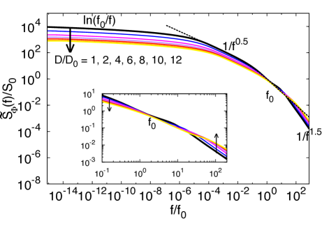
Figure 1: (color online). Theoretical calculation of flux noise due to spin-diffusion in a rectangular SQUID of sides $L_{\parallel}$ and $L_{\perp}$, with wire width $W$ (we used $L_{\parallel}/L_{\perp}=350/3$ and $L_{\perp}/W=3$ to compare to the experiments below). The solid curves show $\tilde{S}_{\Phi}(f)$ for a range of $D$. The axes are normalized to $f_{0}$ and $S_{0}\equiv\tilde{S}_{\Phi}(f_{0})$, where $f_{0}$ is chosen to be the point where the curves appear to cross. We also normalize $D$ by the quantity $D_{0}=2\pi W^{2}f_{0}$. The dashed line shows the fitting function used in Eq. (12). Inset: A zoom into the crossing band region at $f_{0}$. The arrows show the behavior for increasing $D$. At frequencies lower than $f_{0}$, the noise spectral density decreases with increasing $D$; at frequencies higher than $f_{0}$ the opposite behaviour takes place.

In Figure 1 we show the noise power spectral density calculated for our SQUID geometry using Eq. (10) for a range of $D$. The axes are normalized to $f_{0}$ and $S_{0}\equiv\tilde{S}(f_{0})$, where $f_{0}$ is chosen to be the point where the curves appear to cross. We also normalize $D$ by the quantity $D_{0}=2\pi W^{2}f_{0}$ (note that $f_{0}$ coincides with $f_{c}$ when $D=D_{0}$).

At low frequencies ($f<10^{-5}f_{0}$), the noise scales logarithmically as $\ln{(f_{0}/f)}$, flattening out due to the finite size of the SQUID. At intermediate frequencies ($f=10^{-4}-10^{-1}f_{0}$), it varies as $1/f^{0.5}$ over three decades of frequency; at higher frequencies ($f>10f_{0}$), the noise is cut-off as $1/f^{1.5}$.

The low frequency limit of Eq. (9) depends crucially on dimensionality. In 1d, low frequency noise diverges as $1/f^{0.5}$,macfarlane50 ; scofield85 while in 2d it diverges logarithmically as shown in Fig. 1; in 3d the noise flats out as a constant. On the other hand, the high frequency limit of Eq. (9) is $1/f^{1.5}$ for all dimensions. Notably, in all cases the $1/f$ behavior obtained in a previous modelfaoro08 appears only in a narrow frequency band.

The diffusion constant may be temperature dependent. This gives a possible mechanism for the temperature dependence of flux noise observed in several experiments since Ref. wellstood87, . Figure 1 shows plots of the spin-diffusion noise for different values of the diffusion constant $D/D_{0}=1$–$12$. In the range of frequencies $f_{c}=D/(2\pi W^{2})$ the different curves approach each other and a crossing band occurs. The inset of Fig. 1 displays the same calculation focusing on the frequency band where this crossing occurs. $\tilde{S}_{\Phi}(f)$ decreases with increasing $D$ to the left of the crossing band and increases with increasing $D$ in the region to the right of the crossing band.

V Measurements of flux noise

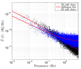
Figure 2: (color online). Typical measurements of low frequency noise. We plot $\tilde{S}_{\Phi}(f)$ vs $f$ for one of the qubits ($q2$) at $T=20$ and $60$ mK. The solid curves show fits to Eq. (11). We observe a crossing at $0.1-1$ Hz across the measured temperature range, roughly consistent with Ref. anton13, .

To test the spin-diffusion model, we performed measurements of flux noise on sixteen compound Josephson junction rf-SQUID flux qubitsharris10 with identical geometries, shown in Fig. 6. The devices were fabricated with a process comprising a Nb/AlOx/Nb trilayer, planarized SiO₂ dielectric layers and Nb wiring layers. The rf-SQUID wires have lateral width $W=1$ $\mu$m, with $L_{\parallel}=350$ $\mu$m and $L_{\perp}=3$ $\mu$m, and are separated by $0.2$ $\mu$m from a Nb ground plane. The sample was mounted to the mixing chamber of a dilution refrigerator with its temperature regulated at set points between $20$ and $80$ mK. We shielded the sample from external magnetic flux with a superconducting Al shield.

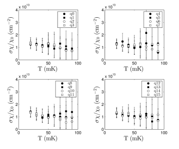
Figure 3: Fit values of $\sigma\chi/\chi_{0}$ versus temperature for sixteen devices. $\sigma\chi/\chi_{0}$ was obtained by fitting the measured power spectral density to Eq. (11). Within the experimental error bars, $\sigma\chi/\chi_{0}$ seems to be independent of temperature and device. For $\chi=\chi_{0}$, this suggests the spin areal density, $\sigma$, is constant.

We measured flux noise using a method described in detail elsewhere.lanting-2009 We directly measured the noise power spectral density $\rm{PSD}(f)$ between $f=1$ mHz and $f=20$ Hz for sixteen devices for temperatures between $20$ mK and $80$ mK. Our measurements have a white noise contribution (i.e. frequency independent) $w_{n}\propto T^{2}$ due to the statistical uncertainty of the noise detection method, as well as the low frequency noise from the devices (Appendix B describes the origin of the white noise background $w_{n}$ and shows that it scales as $T^{2}$). We extract $\tilde{S}_{\Phi}(f)$ by fitting our data to

$${\rm PSD}(f)=\tilde{S}_{\rm analytic}(f)+w_{n},$$ (11)

where $w_{n}$ is this white noise contribution and $\tilde{S}_{\rm analytic}(f)$ is an analytic approximation to Eq. (10) given by

$$\tilde{S}_{\rm analytic}(f)=\left(\frac{\sigma\chi}{\chi_{0}}\right)\frac{F_{0}^{2}L_{\perp}^{2}}{f}\left(1-e^{-\sqrt{\xi 2\pi W^{2}f/D}}\right).$$ (12)

The parameter $\xi=17.6$ is a numerical fit to Eq. (10) calculated for the rf-SQUID geometry discussed above, and $F_{0}=4~{}{\rm n}\Phi_{0}$ is the value of the modulus of the flux vector for surface spins obtained in Appendix A. Equation (12) is shown as a dashed line in Fig. 1, where it is seen to fit the noise spectrum over a limited range of frequencies ($10^{-4}f_{0}<f<10f_{0}$), that turns out to be the relevant range measured in our experiments. We fit our data to Eq. (11) in order to extract the two free parameters, $D$ and $\left(\frac{\sigma\chi}{\chi_{0}}\right)$ independently. See Fig. 2 for typical data at two different temperatures and fits to Eq. (11). Note that the crossing band occurs at $f_{c}=0.1-1$ Hz.

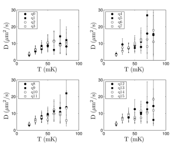
Figure 4: Fit value of the spin-diffusion constant $D$ versus temperature for sixteen devices. $D$ was obtained by fitting the measured power spectral density to Eq. (11). In the low temperature range, $D$ shows a clear trend to increase with temperature. In the higher temperature range the increasing contribution of the white noise background $w_{n}$ increases the error bars making this trend less clear.

Figure 3 shows the fit quantity $\sigma\chi/\chi_{0}$ as a function of temperature for sixteen devices. Within the experimental error bars we see that $\sigma\chi/\chi_{0}=10^{-13}{\rm cm}^{-2}$ is the same constant for all devices, independent of temperature. Plots of $\sqrt{w_{n}}$ as a function of $T$ demonstrate that the qubit and refrigerator thermometry were in agreement even at the lowest temperatures (See Fig. 8 in the Appendix below). Our theory predicts $\sigma\chi/\chi_{0}$ independent of $D$. Hence Fig. 3 shows that $\sigma\chi/\chi_{0}$ is roughly independent of $T$, and that any $T$-dependence must originate from $D(T)$. Assuming $\chi\approx\chi_{0}$ (paramagnetic phase), we get $\sigma=1\times 10^{13}/{\rm cm}^{2}$ for the area density of spins covering the wire (top plus bottom).

Fig. 4 shows the fit parameter $D$, the spin diffusion constant, as a function of $T$ for all sixteen devices. The fit values are in the range of $3-30$ $\mu$m${}^{2}/$s and show a trend of increasing with temperature. We only fit data up to $T=80$ mK. Above this temperature the white noise contribution $w_{n}\propto T^{2}$ begins to dominate across the fit bandwidth and we cannot reliably separate the two terms in Eq. (11) and thus extract the intrinsic flux noise $\tilde{S}_{\Phi}(f)$. At higher temperatures the increasing $w_{n}$ increases the uncertainty on the fit parameters $D$ and $\sigma\chi/\chi_{0}$, as shown by the increasing error bars in Figs. 3 and 4.

For comparison to measurements by other groups, we show measurements of $\tilde{S}_{\Phi}(1~{}{\rm Hz})$ versus temperature for all devices in Fig. 5. Here we see that there is a clear temperature dependence, with the PSD decreasing from $1.8\times 10^{-11}$ $\Phi_{0}^{2}/$Hz to $1\times 10^{-11}$ $\Phi_{0}^{2}/$Hz over this range of temperature.

VI Interpretation of the experiment: Proximity to a phase transition

It is known that $D$ is temperature dependent when the spin system is close to a phase transition.bennet65 ; halperin67 ; sompolinsky81 Assuming $\sigma$ is constant, Fig. 3 suggests that the susceptibility is following the Curie $1/T$ law with no additional temperature dependence. This is consistent with the behavior just above a spin-glass critical temperature $T_{c}$, whose $\chi$ deviates from $\chi_{0}$ by a kink at $T=T_{c}$. The prediction of the theory of dynamical critical phenomena is that $D\propto|T-T_{c}|^{1}$ close to the spin-glass transition.sompolinsky81 Thus the trend in Fig. 4 is consistent with $T>T_{c}$ for a spin-glass phase transition.

The scenario of proximity to a phase transition would also be consistent with previous experiments. It is possible that other fabrication methods will yield devices with extremely low $T_{c}$, so that $T\gg T_{c}$; in this case $D$ will be independent of $T$ and our model leads to flux noise that does not change with temperature, as observed in another recent experiment.yan12 In other samples $T_{c}$ may be higher, leading to additional $T$-dependence in the $T\approx T_{c}$ regime [$\chi\neq\chi_{0}$ in Eq. (9)], where spin-clusters are present as was claimed in Ref. anton13, .

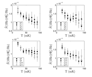
Figure 5: $\tilde{S}_{\Phi}(1{\rm~{}Hz})$ versus $T$ for all sixteen devices. We used the fit parameters shown in Figs. 3 and 4 and Eq. (12) to calculate $\tilde{S}_{\Phi}(1~{}{\rm Hz})$. Note that $\tilde{S}_{\Phi}(1~{}{\rm Hz})$ decreases with increasing $T$.

VII Conclusions

In conclusion, our theory of SQUID flux noise due to the spin-diffusion of interacting spins shows how the frequency and temperature dependence of flux noise is influenced by SQUID geometry and a $T$-dependent spin-diffusion constant, giving rise to the presence of a crossing band of frequencies, like the one observed in a previous experiment.anton13 We presented experimental data in the low temperature range ($T=20-80$ mK), showing that the theory can explain the experiments provided that we assume that the spin-diffusion constant increases with temperature. A temperature dependent spin diffusion constant suggests that the spin system is close to a spin-glass phase transition, but more experiments are needed to confirm this assertion.

We thank C. Dasgupta, P. Kovtun, A.Yu. Smirnov, and N.M. Zimmerman for useful discussions. Our research was supported by the NSERC Engage program.

Appendix A Flux from a spin near SQUID wiring

The devices tested were rf-SQUID flux qubits with superconducting wiring (Nb) in the shape of a rectangular washer, with external sides $L_{\parallel}=350~{}\mu$m and $L_{\perp}=3~{}\mu$m. The washer is made of thin film wires of thickness $b=0.2$ $\mu$m and lateral width $W=1$ $\mu$m (See Fig. 6).

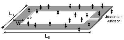
Figure 6: An illustration of the geometry of the rf-SQUID flux qubit wiring used in our theoretical calculations and experimental measurements. Our SQUIDs had wire width $W=1$ $\mu$m, wire thickness $b=0.2$ $\mu$m, and lateral dimensions $L_{\parallel}=350~{}\mu$m and $L_{\perp}=3~{}\mu$m. For simplicity we include a single Josephson junction in the illustration. The measurements reported herein were taken with compound-compound Josephson junction devices described in detail elsewhere harris10 .

We used the analytical expression for the current density flowing through a thin film superconductor (with wire width $W$ much larger than film thickness $b$, just like our SQUID wires). We used the full interpolated expression described in Eqs. (1)–(4) of Ref. vanduzer99, for $\bm{J}_{\rm{SQUID}}(\bm{r})$. The results for $|\bm{F}(\bm{R})|$ as a function of spin position $\bm{R}$ for wire width $W=1$ $\mu$m and wire thickness $b=0.2$ $\mu$m is shown in Fig. 7 below. As a check of the reliability of our results, we performed computations for wires and spin distances similar to the ones considered in Ref. koch07, , confirming that our calculations are in good agreement with previous calculations performed with the software package FastHenry.

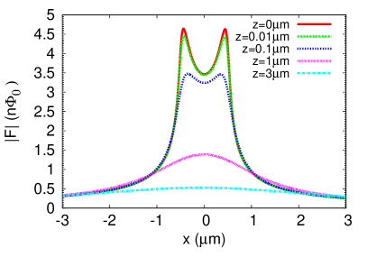
Figure 7: (color online). Calculations of the modulus of the flux vector $\bm{F}(\bm{r})$ as a function of spin position $\bm{r}$ for the rf-SQUID flux qubit geometry of Fig. 6. Here $x$ is the spin’s coordinate along the SC wire width (the wire edges are at $x=\pm W/2$), and $z$ is the spin coordinate perpendicular to the wire ($z=0$ is at the wire surface). Note that at the wire surface, $|\bm{F}|$ is within 20% of $F_{0}=4$ n$\Phi_{0}$.

The qubit wiring is separated by $0.2\ \mu$m from a Nb superconducting ground plane in order to provide magnetic shielding from other flux sources. The effect of this ground plane is to produce a mirror current distribution in the plane below the SQUID. Because of symmetry, the current distribution is not changed (i.e., the current is still peaked at the edge of the SQUID wire). While the ground plane does affect the value of the flux produced by a spin away from the wire surface (e.g. spins in the midpoint between the SQUID and the ground plane will have $\bm{F}=\bm{0}$), it does not significantly affect the value of flux vector $\bm{F}$ for the spins located at the wire surface ($z=0$ in Fig. 7). This happens because for surface spins, the contribution from the mirror current is insignificant in comparison to the contribution from the actual SQUID wire current. Note how in Fig. 7 the value of $|\bm{F}|$ decreases rapidly as the spin-wire distance increases (In Fig. 7 only spins within $\sim 0.1$ $\mu$m of the wire surface produce appreciable flux).

The result that $\bm{F}$ decreases rapidly with increasing spin-wire distance motivates the consideration of a 2d model of surface or interface spins with $\bm{R}_{i}$ in the plane of the wire. In the present calculations we took $|\bm{F}(\bm{R}_{i})|\approx F_{0}$ when $\bm{R}_{i}$ is on the surface of the wire, and $\bm{F}(\bm{R}_{i})=\bm{0}$ elsewhere. In Fig. 7 we see that surface spins have $|\bm{F}|=F_{0}=4\ {\rm n}\Phi_{0}$ apart from an oscillation of 20%.

Appendix B Flux noise measurement details

Here we describe the method used to measure flux noise in more detail. The method was introduced in Ref. lanting-2009, as a method of detecting 1/f noise in situ in superconducting flux qubits. The qubit design is described in detail in Ref. harris10, .

B.1 The CCJJ qubit

The qubits are compound-compound Josephson-Junction (CCJJ) rf-SQUID flux qubits described in Ref. harris10, . Two external flux biases $\Phi_{\rm CCJJ}^{x}$ and $\Phi_{q}^{x}$ allow us to operate the qubit as an effective Ising spin governed by the Hamiltonian:

$${\cal H}=-\frac{1}{2}\left[\epsilon\sigma_{z}+\Delta\sigma_{x}\right],$$ (13)

where $\epsilon=2|I_{q}^{p}|(\Phi_{q}^{x}-\Phi_{q}^{0})$, $|I_{q}^{p}(\Phi_{\rm CCJJ}^{x})|$ is the expectation value of persistent current and $\Delta(\Phi_{\rm CCJJ}^{x})$ is the tunneling amplitude. We anneal the qubit by ramping $\Phi_{\rm CCJJ}$ from $\Phi_{0}/2$ to $\Phi_{0}$ in a time $t_{a}=10\ \mu$s and then read out its state. When the qubit is in thermal equilibrium with a thermal bath at temperature $T$, the probability of detecting state $\left|\uparrow\right\rangle$ is given by:

$$P=\frac{\textrm{e}^{\epsilon/(2k_{B}T)}}{\textrm{e}^{\epsilon/(2k_{B}T)}+\textrm{e}^{-\epsilon/(2k_{B}T)}}=\frac{1}{2}\left[1+\tanh{\left(\frac{\Phi_{q}^{x}-\Phi_{q}^{0}}{2\delta}\right)}\right],$$ (14)

where $\delta$ is given by

$$\delta=\frac{k_{B}T}{2|I_{q}^{p*}|},$$ (15)

and where $|I_{q}^{p*}|$ is the persistent current of the qubit at the point where dynamics cease and the qubit localizes into $\left|\uparrow\right\rangle$ or $\left|\downarrow\right\rangle$.

B.2 Noise Measurement Method

The noise measurement technique is described in detail in Ref. lanting-2009, . In the presence of a low frequency noise signal $\Phi_{n}(t)\ll\delta$, Eq. 14 becomes

$$P=\frac{1}{2}\left[1+\tanh{\left(\frac{\Phi_{n}(t)+\Phi_{q}^{x}-\Phi_{q}^{0}}{2\delta}\right)}\right]$$ (16)

We first calibrate $\Phi_{q}^{0}$ and $\delta$ and then perform measurements of $P(t)$ by setting $\Phi_{q}^{x}=\Phi_{q}^{0}$ and then annealing and reading out the qubit $n$ times. Whenever the outcome is $\left|\uparrow\right\rangle$, we assign a value $P_{i}=1$, and when the outcome is $\left|\downarrow\right\rangle$ we assign $P_{i}=0$. After $n$ anneals we get

$$P=\frac{1}{n}\sum_{i=1}^{n}P_{i}.$$ (17)

We then convert this into a measurement of $\Phi_{n}$ by using Eq. (16). We repeat this procedure $m$ times (a total of $n\times m$ anneals) in order to get a sampling of $\Phi_{n}(t)$ at time intervals $t_{j}=j\Delta t$, $j=1,2,\ldots,m$. Here, $\Delta t=n\tau_{s}$ where $\tau_{s}$ is the time required to anneal and read out the qubit once. We then take the fast Fourier transform of the sample and extract the noise as

$$\tilde{S}_{\Phi}(f_{k})=\frac{1}{m\Delta t}\left|\tilde{\Phi_{n}}(f_{k})\right|^{2},$$ (18)

at frequencies $f_{k}=\frac{k}{m\Delta t}$, $k=-\frac{m}{2}+1,-\frac{m}{2}+2,\ldots,\frac{m}{2}$. The highest frequency is the Nyquist frequency $f_{\rm{Nyquist}}=\frac{1}{2\Delta t}$.

The statistical limit of this noise detection procedure is related to the variance in the measurement of $P$ using Eq. (17). Denoting $p\equiv\langle P\rangle$ for the probability of measuring outcome $P_{i}=1$:

$$\sigma_{P}^{2}=\langle P^{2}\rangle-\langle P\rangle^{2}=\left(\frac{p(1-p)}{n}+p^{2}\right)-p^{2}=\frac{p(1-p)}{n}\approx\frac{1}{4n},$$ (19)

the last approximation when $p\approx 1/2$. This variance will lead to a white noise background $w_{n}$ for the measurement of $\tilde{S}_{\Phi}(f)$. To compute $w_{n}$ note that

$$\langle\Phi_{n}^{2}\rangle=\left(4\delta\right)^{2}\sigma_{P}^{2}=\frac{4\delta^{2}}{n}=\int_{-f_{\rm{Nyquist}}}^{f_{\rm{Nyquist}}}w_{n}=2f_{\rm{Nyquist}}w_{n}.$$ (20)

We can then obtain an expression for $w_{n}$:

$$w_{n}=4\tau_{s}\delta^{2}\propto T^{2}.$$ (21)

The result that $w_{n}$ scales with temperature squared gives a useful means of comparing qubit temperature and refrigerator temperature. Figure 8 shows a plot of $\sqrt{w_{n}}$ as a function of $T$. The linear relation evident in Figure 8 is direct evidence that the qubit is in thermal equilibrium with its environment at all temperatures investigated.

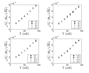
Figure 8: Plots of $\sqrt{w_{n}}$ vs. refrigerator thermometry $T$ for sixteen qubits. The data scale as expected from Eq. 21, direct evidence that the qubit temperature matches the refrigerator temperature. Note in particular that $\sqrt{w_{n}}$ does not saturate at low $T$, demonstrating that the qubit temperature and refrigerator thermometry are in agreement even at the lowest temperatures.

References

- (1) J. Clarke and F.K. Wilhelm, Nature 453, 1031 (2008).
- (2) R.H. Koch, D.P. DiVincenzo, and J. Clarke, Phys. Rev. Lett. 98, 267003 (2007).
- (3) R.C. Bialczak, R. McDermott, M. Ansmann, M. Hofheinz, N. Katz, E. Lucero, M. Neeley, A.D. O’Connell, H. Wang, A.N. Cleland, and J.M. Martinis, Phys. Rev. Lett. 99, 187006 (2007).
- (4) S. Sendelbach, D. Hover, A. Kittel, M. Mück, J.M. Martinis, and R. McDermott, Phys. Rev. Lett. 100, 227006 (2008).
- (5) F. Yoshihara, Y. Nakamura, and J.S. Tsai,Phys. Rev. B81, 132502 (2010).
- (6) F. Yan, J. Bylander, S. Gustavsson, F. Yoshihara, K. Harrabi, D.G. Cory, T.P. Orlando, Y. Nakamura, J.-S. Tsai, and W.D. Oliver, Phys. Rev. B85, 174521 (2012).
- (7) Z. Chen and C.C. Yu, Phys. Rev. Lett. 104, 247204 (2010).
- (8) R. de Sousa, Phys. Rev. B76, 245306 (2007).
- (9) S.K. Choi, D.-H. Lee, S.G. Louie, and J. Clarke, Phys. Rev. Lett. 103, 197001 (2009).
- (10) L. Faoro and L.B. Ioffe, Phys. Rev. Lett. 100, 227005 (2008).
- (11) F.C. Wellstood, C. Urbina, and J. Clarke, Appl. Phys. Lett. 50, 772 (1987).
- (12) S.M. Anton, J.S. Birenbaum, S.R. O’Kelley, V. Bolkhovsky, D.A. Braje, G. Fitch, M. Neeley, G.C. Hilton, H.-M. Cho, K.D. Irwin, F.C. Wellstood, W.D. Oliver, A. Shnirman, and John Clarke, Phys. Rev. Lett. 110, 147002 (2013).
- (13) J.D. Jackson, Classical Electrodynamics, third edition (Wiley, New York, USA 1999).
- (14) T. van Duzer and C.W. Turner, Principles of superconductive devices and circuits (Prentice Hall, New Jersey, USA 1999).
- (15) This is the so called “model J” in the theory of dynamic critical phenomena, see Section 8.6 in P.M. Chaikin and T.C. Lubensky, Principles of condensed matter physics (Cambridge University Press, Cambridge U.K., 2000).
- (16) H.S. Bennet and P.C. Martin, Phys. Rev. 138, A608 (1965).
- (17) M.B. Weissman, Rev. Mod. Phys. 60, 537 (1988).
- (18) T. Lanting et al., Phys. Rev. B79 060509 (2009).
- (19) G.G. Macfarlane, Proc. Phys. Soc. Lond. B 63, 807 (1950).
- (20) J.H. Scofield and W.W. Webb, Phys. Rev. Lett. 54, 353 (1985).
- (21) R. Harris et al., Phys. Rev. B81, 134510 (2010).
- (22) B.I. Halperin and P.C. Hohenberg, Phys. Rev. Lett. 19, 700 (1967).
- (23) H. Sompolinsky and A. Zippelius, Phys. Rev. Lett. 47, 359 (1981).