Tight Lower Bound on the Probability of a Binomial Exceeding its Expectation

Abstract

We give the proof of a tight lower bound on the probability that a binomial random variable exceeds its expected value. The inequality plays an important role in a variety of contexts, including the analysis of relative deviation bounds in learning theory and generalization bounds for unbounded loss functions.

1 Motivation

This paper presents a tight lower bound on the probability that a binomial random variable exceeds its expected value. If the binomial distribution were symmetric around its mean, such a bound would be trivially equal to $\frac{1}{2}$. And indeed, when the number of trials $m$ for a binomial distribution is large, and the probability $p$ of success on each trial is not too close to $0$ or to $1$, the binomial distribution is approximately symmetric. With $p$ fixed, and $m$ sufficiently large, the de Moivre-Laplace theorem tells us that we can approximate the binomial distribution with a normal distribution. But, when $p$ is close to $0$ or $1$, or the number of trials $m$ is small, substantial asymmetry around the mean can arise. Figure 1 illustrates this by showing the binomial distribution for different values of $m$ and $p$.

The lower bound we prove has been invoked several times in the machine learning literature, starting with work on relative deviation bounds by Vapnik [8], where it is stated without proof. Relative deviation bounds are useful bounds in learning theory that provide more insight than the standard generalization bounds because the approximation error is scaled by the square root of the true error. In particular, they lead to sharper bounds for empirical risk minimization, and play a critical role in the analysis of generalization bounds for unbounded loss functions [2].

This binomial inequality is mentioned and used again without proof or reference in [1], where the authors improve the original work of [8] on relative deviation bounds by a constant factor. The same claim later appears in [9] and implicitly in other publications referring to the relative deviations bounds of Vapnik [8].

To the best of our knowledge, there is no publication giving an actual proof of this inequality in the machine learning literature. Our search efforts for a proof in the statistics literature were also unsuccessful. Instead, some references suggest that such a proof is indeed not available. In particular, we found one attempt to prove this result in the context of the analysis of some generalization bounds [3], but unfortunately the proof is not sufficient to show the general case needed for the proof of Vapnik [8], and only pertains to cases where the number of Bernoulli trials is ‘large enough’. No paper we have encountered contains a proof of the full theorem. Our proof therefore seems to be the first rigorous justification of this inequality in its full generality, which is needed for the analysis of relative deviation bounds in machine learning.

In Section 2, we start with some preliminaries and then give the presentation of our main result. In Section 3, we give a detailed proof of the inequality.

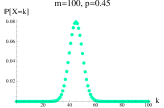
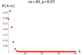
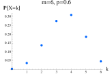
Figure 1: Plots of the probability of getting different numbers of successes k, for the binomial distribution $B(m,p)$, shown for three different values of $m$, the number of trials, and $p$, the probability of a success on each trial. Note that in the second and third image, the distribution is clearly not symmetrical around its mean.

2 Main result

The following is the standard definition of a binomial distribution.

Definition 1

A random variable $X$ is said to be distributed according to the binomial distribution with parameters $m$ (the number of trials) and $p$ (the probability of success on each trial), if for $k=0,1,\ldots,m$ we have

$$\mathbb{P}[X=k]=\binom{m}{k}p^{k}(1-p)^{m-k}.$$ (1)

The binomial distribution with parameters $m$ and $p$ is denoted by $B(m,p)$. It has mean $mp$ and variance $mp(1-p)$.

The following theorem is the main result of this paper.

Theorem 2.1

For any positive integer $m$ and any probability p such that $p>\frac{1}{m}$, let $X$ be a random variable distributed according to $B(m,p)$. Then, the following inequality holds:

$$\mathbb{P}\big{[}X\geq\operatorname*{\mathbb{E}}\left[X\right]\big{]}>\frac{1}{4},$$ (2)

where $\operatorname*{\mathbb{E}}[X]=mp$ is the expected value of $X$.

The lower bound is never reached but is approached asymptotically when $m=2$ as $p\to\frac{1}{2}$ from the right. Note that when $m=2$, the case $p=\frac{1}{2}$ is excluded from consideration, due to our assumption $p>\frac{1}{m}$. In words, the theorem says that a coin that is flipped a fixed number of times always has a probability of more than $\frac{1}{4}$ of getting at least as many heads as the expected value of the number of heads, as long as the coin’s chance of getting a head on each flip is not so low that the expected value is less than or equal to 1. The inequality is tight, as illustrated by Figure 2. In corollary 3 we prove a bound on the probability of a binomial random variable being less than or equal to its expected value, which is very similar to the bound here on such a random variable being greater than or equal to its expected value.

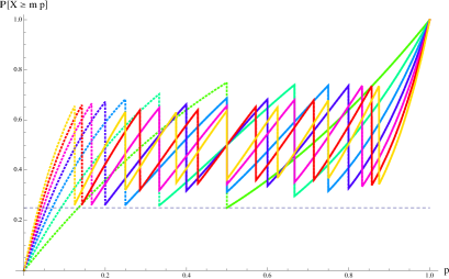
Figure 2: This plot depicts $\mathbb{P}[X\geq\operatorname*{\mathbb{E}}[X]]$, the probability that a binomially distributed random variable $X$ exceeds its expectation, as a function of the trial success probability $p$. Each colored line corresponds to a different number of trials, $m=2,3,\ldots,8$. Each colored line is dotted in the region where $p\leq\frac{1}{m}$, and solid in the region that our proof pertains to, where $p>\frac{1}{m}$. The dashed horizontal line at $\frac{1}{4}$ represents the value of the lower bound. Our theorem is equivalent to saying that for all positive integers $m$ (not just the values of $m$ shown in the plot), the solid portions of the colored lines never cross below the dashed horizontal line. As can be seen from the figure, the lower bound is nearly met for many values of $m$.

3 Proof

Our proof of theorem 2.1 is based on the following series of lemmas and corollaries and makes use of Camp-Paulson’s normal approximation to the binomial cumulative distribution function [6, 5, 7]. We start with a lower bound that reduces the problem to a simpler one.

Lemma 1

For all $k=1,2,\ldots,m-1$ and $p\in(\frac{k}{m},\frac{k+1}{m}]$, the following inequality holds:

$$\mathbb{P}_{X\sim B(m,p)}[X\geq\operatorname*{\mathbb{E}}[X]]\geq\mathbb{P}_{X\sim B(m,\frac{k}{m})}[X\geq k+1].$$

• Let $X$ be a random variable distributed according to $B(m,p)$ and let $F(m,p)$ denote $\mathbb{P}[X\geq\operatorname*{\mathbb{E}}[X]]$. Since $\operatorname*{\mathbb{E}}[X]=mp$, $F(m,p)$ can be written as the following sum:

  $$F(m,p)=\sum_{j=\lceil mp\rceil}^{m}\binom{m}{j}p^{j}(1-p)^{m-j}.$$

  We will consider the smallest value that $F(m,p)$ can take for $p\in(\frac{1}{m},1]$ and $m$ a positive integer. Observe that if we restrict $p$ to be in the half open interval $I_{k}=(\frac{k-1}{m},\frac{k}{m}]$, which represents a region between the discontinuities of $F(m,p)$ which result from the factor $\lceil mp\rceil$, then we have $mp\in(k-1,k]$ and so $\lceil mp\rceil=k$. Thus, we can write

  $$\forall p\in I_{k},\hskip 4.83694pt\forall k=0,1,\ldots,m-1\quad F(m,p)=\sum_{j=k}^{m}\binom{m}{j}p^{j}(1-p)^{m-j}.$$

  The function $p\mapsto F(m,p)$ is differentiable for all $p\in I_{k}$ and its differential is

  $$\frac{\partial F(m,p)}{\partial p}=\sum_{j=k}^{m}\binom{m}{j}(1-p)^{m-j-1}p^{j-1}(j-mp).$$

  Furthermore, for $p\in I_{k}$, we have $k\geq mp$, therefore $j\geq mp$ (since in our sum $j\geq k$), and so $\frac{\partial F(m,p)}{\partial p}\geq 0$. The inequality is in fact strict when $p\neq 0$ and $p\neq 1$ since the sum must have at least two terms and at least one of these terms must be positive. Thus, the function $p\mapsto F(m,p)$ is strictly increasing within each $I_{k}$. In view of that, the value of $F(m,p)$ for $p\in I_{k+1}$ is lower bounded by $\lim_{p\to\left(\frac{k}{m}\right)^{+}}F(m,p)$, which is given by

  $$\lim_{p\to\left(\frac{k}{m}\right)^{+}}F(m,p)=\sum_{j=k+1}^{m}\binom{m}{j}\left(\frac{k}{m}\right)^{j}\left(1-\frac{k}{m}\right)^{m-j}=\mathbb{P}_{X\sim B(m,\frac{k}{m})}[X\geq k+1].$$

  Therefore, for $k=1,2,\ldots,m-1$, whenever $p\in(\frac{k}{m},\frac{k+1}{m}]$ we have

  $$F(m,p)\geq\mathbb{P}_{X\sim B(m,\frac{k}{m})}[X\geq k+1].$$ ∎

Corollary 1

For all $p\in(\frac{1}{m},1)$, the following inequality holds:

$$\mathbb{P}_{X\sim B(m,p)}[X\geq\operatorname*{\mathbb{E}}[X]]\geq 1-\max_{k\in\{1,\ldots,m-1\}}\mathbb{P}_{X\sim B(m,\frac{k}{m})}[X\leq k].$$

Proof

By Lemma 1, the following inequality holds

$$\mathbb{P}_{X\sim B(m,p)}[X\geq\operatorname*{\mathbb{E}}[X]]\geq\min_{k\in\{1,..,m-1\}}\mathbb{P}_{X\sim B(m,\frac{k}{m})}[X\geq k+1].$$

The right-hand side is equivalent to

$$\min_{k\in\{1,..,m-1\}}1-\mathbb{P}_{X\sim B(m,\frac{k}{m})}[X\leq k]=1-\max_{k\in\{1,\ldots,m-1\}}\mathbb{P}_{X\sim B(m,\frac{k}{m})}[X\leq k]$$

which concludes the proof.

In view of Corollary 1, in order to prove our main result it suffices that we upper bound the expression

$$\mathbb{P}_{X\sim B(m,\frac{k}{m})}[X\leq k]=\sum_{j=0}^{k}\binom{m}{j}\left(\frac{k}{m}\right)^{j}\left(1-\frac{k}{m}\right)^{m-j}$$

by $\frac{3}{4}$ for all integers $m\geq 2$ and $1\leq k\leq m-1$. Note that the case $m=1$ is irrelevant since the inequality $p>\frac{1}{m}$ assumed for our main result cannot hold in that case, due to $p$ being a probability. The case $k=0$ can also be ignored since it corresponds to $p\leq\frac{1}{m}$. Finally, the case $k=m$ is irrelevant, since it corresponds to $p>1$. We note, furthermore, that when $p=1$ that immediately gives $\mathbb{P}_{X\sim B(m,p)}[X\geq\operatorname*{\mathbb{E}}[X]]=1\geq\frac{1}{4}$.

Now, we introduce some lemmas which will be used to prove our main result.

Lemma 2

The following inequality holds for all $k=1,2,\ldots,m-1$:

$$\mathbb{P}_{X\sim B(m,\frac{k}{m})}[X\leq k]\leq\Phi\left[\frac{\beta_{k}\theta+\frac{1}{3}\gamma_{m,k}}{\sqrt{\beta_{k}+\gamma_{m,k}}}\right]+\frac{0.007}{\sqrt{1-\frac{1}{m}}},$$

where $\Phi\colon x\mapsto\int_{-\infty}^{x}\frac{1}{\sqrt{2\pi}}e^{\frac{-s^{2}}{2}}ds$ is the cumulative distribution function for the standard normal distribution and $\beta_{k}$, $\gamma_{m,k}$, and $\theta$ are defined as follows:

$$\beta_{k}=\frac{1}{1+k}\left(1+\frac{1}{k}\right)^{2/3}\mspace{-25.0mu},\quad\gamma_{m,k}=\frac{1}{m-k},\quad\theta=\frac{17}{3\ 2^{1/3}}-3\ 2^{1/3}\approx 0.71787.$$

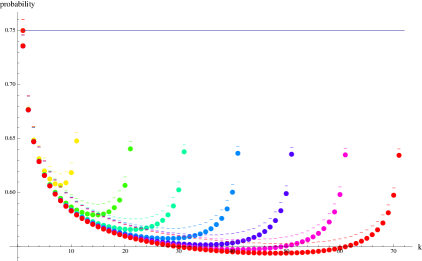
Figure 3: For m=2, 22, $\ldots$, 72 and $1\leq k\leq m-1$, this plot depicts the values of $\mathbb{P}_{X\sim B(m,\frac{k}{m})}[X\leq k]$ as colored dots (with one color per choice of m), against the values of the bound from Lemma 2, which are shown as short horizontal lines of matching color. The upper bound that we need to demonstrate, $\frac{3}{4}$, is shown as a blue horizontal line.

Proof

Our proof makes use of Camp-Paulson’s normal approximation to the binomial cumulative distribution function [6, 5, 7], which helps us reformulate the bound sought in terms of the normal distribution. The Camp-Paulson approximation improves on the classical normal approximation by using a non-linear transformation. This is useful for modeling the asymmetry that can occur in the binomial distribution. The Camp-Paulson bound can be stated as follows [6, 5]:

$$\left|\mathbb{P}_{X\sim B(m,p)}[X\leq j]-\Phi\Big{[}\frac{c-\mu}{\sigma}\Big{]}\right|\leq\frac{0.007}{\sqrt{mp(1-p)}}$$

where

$$c=(1-b)r^{1/3},\quad\mu=1-a,\quad\sigma=\sqrt{br^{2/3}+a},$$

$$a=\frac{1}{9m-9j},\quad b=\frac{1}{9j+9},\quad r=\frac{(j+1)(1-p)}{mp-jp}.$$

Plugging in the definitions for all of these variables yields

$$\Phi\left[\frac{c-\mu}{\sigma}\right]=\Phi\left[\frac{\left(1-\frac{1}{9}\frac{1}{j+1}\right)\left(\frac{1}{p}\frac{(j+1)(1-p)}{m-j}\right)^{1/3}+\frac{1}{9}\frac{1}{m-j}-1}{\sqrt{\frac{1}{9}\frac{1}{j+1}\left(\frac{1}{p}\frac{(j+1)(1-p)}{m-j}\right)^{2/3}+\frac{1}{9}\frac{1}{m-j}}}\right].$$

Applying this bound to the case of interest for us where $p=\frac{k}{m}$ and $j=k$, yields

$$\frac{c-\mu}{\sigma}=\frac{\alpha_{k}+\frac{1}{3}\gamma_{m,k}}{\sqrt{\beta_{k}+\gamma_{m,k}}},$$

with $\alpha_{k}=\left(1+\frac{1}{k}\right)^{1/3}\left(3-\frac{1}{3}\frac{1}{1+k}\right)-3$, and with $\beta_{k}=\frac{1}{1+k}(1+\frac{1}{k})^{2/3}$. Thus, we can write

$$\mathbb{P}_{X\sim B(m,\frac{k}{m})}[X\leq k]\leq\Phi\left[\frac{\alpha_{k}+\frac{1}{3}\gamma_{m,k}}{\sqrt{\beta_{k}+\gamma_{m,k}}}\right]+\frac{0.007}{\sqrt{k\left(1-\frac{k}{m}\right)}}.$$ (3)

To simplify this expression, we will first upper bound $\alpha_{k}$ in terms of $\beta_{k}$. To do so, we consider the ratio

$$\frac{\alpha_{k}}{\beta_{k}}=\frac{(1+\frac{1}{k})^{1/3}(3-\frac{1}{3}\frac{1}{1+k})-3}{\frac{1}{1+k}(1+\frac{1}{k})^{2/3}}=\frac{3[(1+\frac{1}{k})^{1/3}-1]}{\frac{1}{1+k}(1+\frac{1}{k})^{2/3}}-\frac{1}{3(1+\frac{1}{k})^{1/3}}.$$

Let $\lambda=(1+\frac{1}{k})^{1/3}$, which we can rearrange to write $\frac{1}{1+k}=\frac{\lambda^{3}-1}{\lambda^{3}}$, with $\lambda\in(1,2^{1/3}]$. Then, the ratio can be rewritten as follows:

$$\frac{\alpha_{k}}{\beta_{k}}=\frac{3\lambda^{3}[(\lambda-1]}{(\lambda^{3}-1)\lambda^{2}}-\frac{1}{3\lambda}=\frac{3\lambda}{1+\lambda+\lambda^{2}}-\frac{1}{3\lambda}.$$

The expression is differentiable and its differential is given by

$$\frac{d}{d\lambda}\frac{\alpha_{k}}{\beta_{k}} =\frac{3(1+\lambda+\lambda^{2})-3\lambda(2\lambda+1)}{(1+\lambda+\lambda^{2})^{2}}+\frac{1}{3\lambda^{2}}$$

$$=\frac{(1-\lambda^{2})}{(1+\lambda+\lambda^{2})^{2}}+\frac{1}{3\lambda^{2}}=\frac{-8(\lambda-1)^{4}-30(\lambda-1)^{3}-30(\lambda-1)^{2}+9}{3\lambda^{2}\left(1+\lambda+\lambda^{2}\right)^{2}}.$$

For $\lambda\in(1,2^{\frac{1}{3}}]$, $\lambda-1\leq 2^{\frac{1}{3}}-1$ $\leq 0.26$, thus, the following inequality holds:

$$8(\lambda-1)^{4}+30(\lambda-1)^{3}+30(\lambda-1)^{2}\leq 8(2^{\frac{1}{3}}-1)^{4}+30(2^{\frac{1}{3}}-1)^{3}+30(2^{\frac{1}{3}}-1)^{2}\approx 2.59<9.$$

Thus, the derivative is positive, so $\frac{\alpha_{k}}{\beta_{k}}$ is an increasing function of $\lambda$ on the interval $(1,2^{\frac{1}{3}}]$ and its maximum is reached for $\lambda=2^{\frac{1}{3}}$. For that choice of $\lambda$, the ratio can be written

$$\frac{3\ 2^{\frac{1}{3}}}{1+2^{\frac{1}{3}}+2^{\frac{2}{3}}}-\frac{1}{3\ 2^{\frac{1}{3}}}=\frac{17}{3\ 2^{\frac{1}{3}}}-3\ 2^{\frac{1}{3}}=\theta\approx 0.717874,$$

which upper bounds $\frac{\alpha_{k}}{\beta_{k}}$. Since $\Phi[x]$ is a strictly increasing function, using
$\alpha_{k}\leq\theta\beta_{k}$ yields

$$\Phi\left[\frac{\alpha_{k}+\frac{1}{3}\gamma_{m,k}}{\sqrt{\beta_{k}+\gamma_{m,k}}}\right]\leq\Phi\left[\frac{\beta_{k}\theta+\frac{1}{3}\gamma_{m,k}}{\sqrt{\beta_{k}+\gamma_{m,k}}}\right].$$ (4)

We now bound the term $\frac{0.007}{\sqrt{k(1-\frac{k}{m})}}$. The quadratic function $k\mapsto k(1-\frac{k}{m})$ for $k=1,2,\ldots,m-1$, achieves its minimum at $k=1$, giving $k(1-\frac{k}{m})\geq(1-\frac{1}{m})$. Thus, in view of (3) and (4), we can write

$$\mathbb{P}\left[B(m,\frac{k}{m})\leq k\right]\leq\Phi\left[\frac{\beta_{k}\theta+\frac{1}{3}\gamma_{m,k}}{\sqrt{\beta_{k}+\gamma_{m,k}}}\right]+\frac{0.007}{\sqrt{1-\frac{1}{m}}}.$$

This concludes the proof.∎

Lemma 3

Let $\beta_{k}=\frac{1}{1+k}\left(1+\frac{1}{k}\right)^{2/3}$ and $\gamma_{m,k}=\frac{1}{m-k}$ for $m>1$ and
$k=1,2,\ldots,m-1$. Then, the following inequality holds for $\theta=\frac{17}{3\ 2^{\frac{1}{3}}}-3\ 2^{\frac{1}{3}}$:

$$\Phi\left[\frac{\beta_{k}\theta+\frac{1}{3}\gamma_{m,k}}{\sqrt{\beta_{k}+\gamma_{m,k}}}\right]\leq\Phi\left[\frac{\beta_{k}\theta+\frac{1}{3}}{\sqrt{\beta_{k}+1}}\right].$$

Proof

Since for $k=1,2,\ldots,m-1$, we have $\frac{1}{m-1}\leq\gamma_{m,k}\leq 1$, the following inequality holds:

$$\frac{\beta_{k}\theta+\frac{1}{3}\gamma_{m,k}}{\sqrt{\beta_{k}+\gamma_{m,k}}}\leq\max_{\gamma\in[0,1]}\frac{\beta_{k}\theta+\frac{1}{3}\gamma}{\sqrt{\beta_{k}+\gamma}}.$$

Since $\beta_{k}=\frac{1}{1+k}\left(1+\frac{1}{k}\right)^{2/3}>0$, the function $\phi\colon\gamma\mapsto\frac{\beta_{k}\theta+\frac{1}{3}\gamma}{\sqrt{\beta_{k}+\gamma}}$ is continuously differentiable for $\gamma\in[0,1]$. Its derivative is given by $\phi^{\prime}(\gamma)=\frac{\gamma+\beta_{k}(2-3\theta)}{6\left(\beta_{k}+\gamma\right){}^{3/2}}$. Since
$2-3\theta\approx-0.1536<0$, $\phi^{\prime}(\gamma)$ is non-negative if and only if $\gamma\geq\beta_{k}(3\theta-2)$. Thus, $\phi(\gamma)$ is decreasing for $\gamma<\beta_{k}(3\theta-2)$ and increasing for values of $\gamma$ larger than that threshold. That implies that the shape of the graph of $\phi(\gamma)$ is such that the function’s value is maximized at the end points. So $\max_{\gamma\in[0,1]}\phi(\gamma)=$ $\max(\phi(0),\phi(1))=\max(\sqrt{\beta_{k}}\theta,\frac{\beta_{k}\theta+\frac{1}{3}}{\sqrt{\beta_{k}+1}})$. The inequality $\sqrt{\beta_{k}}\theta\leq\frac{\beta_{k}\theta+\frac{1}{3}}{\sqrt{\beta_{k}+1}}$ holds if and only if $\beta_{k}(\beta_{k}+1)\theta^{2}\leq(\beta_{k}\theta+\frac{1}{3})^{2}$, that is if $\beta_{k}\leq\frac{1}{\theta(9\theta-6)}\approx 3.022$. But since $\beta_{k}$ is a decreasing function of $k$, it has $\beta_{1}\approx 0.7937$ as its upper bound, and so this necessary requirement always holds. That means that the maximum value of $\phi(\gamma)$ for $\gamma\in[0,1]$ occurs at $\gamma=1$, yielding the upper bound $\frac{\beta_{k}\theta+\frac{1}{3}}{\sqrt{\beta_{k}+1}}$, which concludes the proof.

Corollary 2

The following inequality holds for all $m\geq 2$ and $k\geq 2$:

$$\mathbb{P}_{X\sim B(m,\frac{k}{m})}[X\leq k]\leq 0.7152.$$

Proof

By Lemmas 2-3, we can write

$$\mathbb{P}_{X\sim B(m,\frac{k}{m})}[X\leq k]\leq\Phi\left[\frac{\beta_{k}\theta+\frac{1}{3}}{\sqrt{\beta_{k}+1}}\right]+\frac{0.007}{\sqrt{1-\frac{1}{m}}}.$$

Furthermore $\beta_{k}=\frac{1}{1+k}\left(1+\frac{1}{k}\right)^{2/3}$ is a decreasing function of $k$. Therefore, for $k\geq 2$, it must always be within the range $\beta_{k}\in\left[\lim_{k\to\infty}\beta_{k},\beta_{2}\right]$ = $\left[0,\frac{1}{2^{2/3}3^{1/3}}\right]\approx[0,0.43679]$, which implies

$$\frac{\beta_{k}\theta+\frac{1}{3}}{\sqrt{\beta_{k}+1}}\leq\max_{k\geq 2}\frac{\beta_{k}\theta+\frac{1}{3}}{\sqrt{\beta_{k}+1}}\leq\max_{\beta\in[0,\beta_{2}]}\frac{\beta\theta+\frac{1}{3}}{\sqrt{\beta+1}}.$$

The derivative of the differentiable function $g\colon\beta\mapsto\frac{\beta\theta+\frac{1}{3}}{\sqrt{\beta+1}}$ is given by $g^{\prime}(\beta)=\frac{3(\beta+2)\theta-1}{6(\beta+1)^{3/2}}$. We have that $3(\beta+2)\theta-1\geq 6\theta-1\geq 6\times.717-1>0$, thus $g^{\prime}(\beta)\geq 0$. Hence, the maximum of $g(\beta)$ occurs at $\beta_{2}$, where $g(\beta_{2})$ is slightly smaller than $0.53968$. Thus, we can write

$$\Phi\left[\frac{\beta_{k}\theta+\frac{1}{3}}{\sqrt{\beta_{k}+1}}\right]\leq\Phi\left[\underset{\beta\in\left[0,\beta_{2}\right]}{\max}\frac{\beta\theta+\frac{1}{3}}{\sqrt{\beta+1}}\right]\leq\Phi[0.53968]<0.7053.$$

Now, $m\mapsto\frac{0.007}{\sqrt{1-\frac{1}{m}}}$ is a decreasing of function of $m$, thus, for $m\geq 2$ it is maximized at $m=2$, yielding $\frac{0.007}{\sqrt{1-\frac{1}{m}}}\leq 0.0099$. Hence, the following holds:

$$\Phi\left[\frac{\beta_{k}\theta+\frac{1}{3}}{\sqrt{\beta_{k}+1}}\right]+\frac{0.007}{\sqrt{1-\frac{1}{m}}}\leq 0.7053+0.0099=0.7152,$$

as required.∎

The case $k=1$ is addressed by the following lemma.

Lemma 4

Let $X$ be a random variable distributed according to $B(m,\frac{1}{m})$. Then, the following equality holds for any $m\geq 2$:

$$\mathbb{P}\left[X\leq 1\right]\leq\frac{3}{4}.$$

Proof

For $m\geq 2$, define the function $\rho$ by

$$\rho(m)=\mathbb{P}\left[X\leq 1\right]=\sum_{j=0}^{1}\binom{m}{j}\left(\frac{1}{m}\right)^{j}\left(1-\frac{1}{m}\right)^{m-j}\mspace{-10.0mu}=\left(1-\frac{1}{m}\right)^{m}+\left(1-\frac{1}{m}\right)^{m-1}\mspace{-30.0mu}.$$

The value of the function for $m=2$ is given by $\rho(2)=\left(1-\frac{1}{2}\right)^{2}+\left(1-\frac{1}{2}\right)^{2-1}=\frac{3}{4}.$ Thus, to prove the result, it suffices to show that $\rho$ is non-increasing for $m\geq 2$. The derivative of $\rho$ is given for all $m\geq 2$ by

$$\rho^{\prime}(m)=(m-1)^{m-1}m^{-m}\left(2+(2m-1)\log\left[1-\frac{1}{m}\right]\right).$$

Thus, for $m\geq 2$, $\rho^{\prime}(m)\leq 0$ if and only if $2+(2m-1)\log\left[1-\frac{1}{m}\right]\leq 0$. Now, for $m\geq 2$, using the first three terms of the expansion $-\log\left[1-\frac{1}{m}\right]=\sum_{k=1}^{\infty}\frac{1}{k}\frac{1}{m^{k}}$, we can write

$$-(2m-1)\log\bigg{[}1-\frac{1}{m}\bigg{]}\geq(2m-1)\left(\frac{1}{m}+\frac{1}{2m^{2}}+\frac{1}{3m^{3}}\right)=2+\frac{1}{6m^{2}}-\frac{1}{3m^{3}}\geq 2,$$

where the last inequality follows from $\frac{1}{6m^{2}}-\frac{1}{3m^{3}}\geq 0$ for $m\geq 2$. This shows that $\rho^{\prime}(m)\leq 0$ for all $m\geq 2$ and concludes the proof. ∎

We now complete the proof of our main result, by combining the previous lemmas and corollaries.

Proof (of Theorem 2.1)

By Corollary 1, we can write

$$\mathbb{P}_{X\sim B(m,p)}[X\geq\operatorname*{\mathbb{E}}[X]]$$

$$\geq 1-\max_{k\in\{1,\ldots,m-1\}}\mathbb{P}_{X\sim B(m,\frac{k}{m})}[X\leq k]$$

$$=1-\max\Big{\{}\mathbb{P}_{X\sim B(m,\frac{1}{m})}[X\leq 1],\max_{k\in\{2,\ldots,m-1\}}\mathbb{P}_{X\sim B(m,\frac{k}{m})}[X\leq k]\Big{\}}$$

$$\geq 1-\max\{\frac{3}{4},0.7152\}=1-\frac{3}{4}=\frac{1}{4},$$

where the last inequality holds by Corollary 2 and Lemma 4.∎

As a corollary, we can produce a bound on the probability that a binomial random variable is less than or equal to its expected value, instead of greater than or equal to its expected value.

Corollary 3

For any positive integer $m$ and any probability p such that
$p<1-\frac{1}{m}$, let $X$ be a random variable distributed according to $B(m,p)$. Then, the following inequality holds:

$$\mathbb{P}\big{[}X\leq\operatorname*{\mathbb{E}}\left[X\right]\big{]}>\frac{1}{4},$$ (5)

where $\operatorname*{\mathbb{E}}[X]=mp$ is the expected value of $X$.

Proof

Let $G(m,p)$ be defined as

$$G(m,p)\equiv\mathbb{P}\big{[}X\leq\operatorname*{\mathbb{E}}\left[X\right]\big{]}=\sum_{j=0}^{\lfloor mp\rfloor}\binom{m}{j}p^{j}(1-p)^{m-j}$$

and let $F(m,p)$ be defined as before as

$$F(m,p)\equiv\mathbb{P}\big{[}X\geq\operatorname*{\mathbb{E}}\left[X\right]\big{]}=\sum_{j=\lceil mp\rceil}^{m}\binom{m}{j}p^{j}(1-p)^{m-j}.$$

Then, we can write, for $q=1-p$,

$$G(m,p) =G(m,1-q)$$

$$=\sum_{j=0}^{\lfloor m(1-q)\rfloor}\binom{m}{j}(1-q)^{j}q^{m-j}$$

$$=\sum_{t=m-\lfloor m(1-q)\rfloor}^{m}\binom{m}{m-t}(1-q)^{m-t}q^{t}$$

$$=\sum_{t=\lceil mq\rceil}^{m}\binom{m}{t}(1-q)^{m-t}q^{t}$$

$$=F(m,q)=F(m,1-p)>\frac{1}{4}$$

with the inequality at the end being an application of theorem 2.1, which holds so long as $q>\frac{1}{m}$, or equivalently, so long as $p<1-\frac{1}{m}$. ∎

4 Conclusion

We presented a rigorous justification of an inequality needed for the proof of relative deviations bounds in machine learning theory. To our knowledge, no other complete proof of this theorem exists in the literature, despite its repeated use.

References

• [1] M.Β Anthony and J.Β Shawe-Taylor. A result of Vapnik with applications. Discrete Applied Mathematics, 47:207 – 217, 1993.
• [2] C.Β Cortes, Y.Β Mansour, and M.Β Mohri. Learning bounds for importance weighting. In NIPS, Vancouver, Canada, 2010. MIT Press.
• [3] S.Β A. Jaeger. Generalization bounds and complexities based on sparsity and clustering for convex combinations of functions from random classes. Journal of Machine Learning Research, 6:307–340, 2005.
• [4] P.Β Rigollet and X.Β Tong Neyman-Pearson Classification, Convexity and Stochastic Constraints Journal of Machine Learning Research, 12:2831–2855, 2011.
• [5] N.Β Johnson, A.Β Kemp, and S.Β Kotz. Univariate Discrete Distributions. Number v. 3 in Wiley series in probability and Statistics. Wiley & Sons, 2005.
• [6] N.Β Johnson, S.Β Kotz, and N.Β Balakrishnan. Continuous univariate distributions. Number v. 2 in Wiley series in probability and mathematical statistics: Applied probability and statistics. Wiley & Sons, 1995.
• [7] S.Β M. Lesch and D.Β R. Jeske. Some suggestions for teaching about normal approximations to poisson and binomial distribution functions. The American Statistician, 63(3):274–277, 2009.
• [8] V.Β N. Vapnik. Statistical Learning Theory. Wiley-Interscience, 1998.
• [9] V.Β N. Vapnik. Estimation of Dependences Based on Empirical Data. Springer-Verlag, 2006.