A modeling framework for
Ordered Weighted Average Combinatorial Optimization

Abstract

Multiobjective combinatorial optimization deals with problems considering more than one viewpoint or scenario. The problem of aggregating multiple criteria to obtain a globalizing objective function is of special interest when the number of Pareto solutions becomes considerably large or when a single, meaningful solution is required. Ordered Weighted Average or Ordered Median operators are very useful when preferential information is available and objectives are comparable since they assign importance weights not to specific objectives but to their sorted values. In this paper, Ordered Weighted Average optimization problems are studied from a modeling point of view. Alternative integer programming formulations for such problems are presented and their respective domains studied and compared. In addition, their associated polyhedra are studied and some families of facets and new families of valid inequalities presented. The proposed formulations are particularized for two well-known combinatorial optimization problems, namely, shortest path and minimum cost perfect matching, and the results of computational experiments presented and analyzed. These results indicate that the new formulations reinforced with appropriate constraints can be effective for efficiently solving medium to large size instances.

Keywords: Combinatorial Optimization, Multiobjective optimization, Weighted Average Optimization, Ordered median.

1 Introduction

Multiobjective combinatorial optimization deals with problems considering more than one viewpoint or scenario. They inherit the complexity difficulty of their scalar counterparts, but incorporate additional difficulties derived from dealing with partial orders in the objective function space. The standard solution concept is the set of Pareto solutions. However, the number of Pareto solutions can grow exponentially with the size of the instance and the number of objectives. A first approach to overcome this difficulty focuses on a specific subset of the Pareto set, such as, for instance, the supported Pareto solutions (see, for instance, Ehrgott, 2005). Those are the Pareto solutions that optimize linear scalarizations of the different objectives. However, it is possible to exhibit instances for which even the number of supported solutions grows exponentially with the size of the instance. Furthermore, focusing on supported Pareto solutions a priori excludes compromise solutions that could be preferred by the decision maker. For the above reasons, more involved decision criteria have been proposed in the field of multicriteria decision making (Perny and Spanjaard, 2003). These include objectives focusing on one particular compromise solution, which, for tractability and decision theoretic reasons, seem to be better suited when an appropriate aggregation operator is available.

In some cases, a particularly important Pareto solution related to a weighted ordered average aggregating function is sought. Provided that some imprecise preference information on the objectives is available, and that they are comparable, an averaging operator can be used to aggregate the vector of objective values of feasible solutions. The Ordered Median (OM) objective function is very useful in this context since it assigns importance weights not to specific objectives but to their sorted values. OM operators have been successfully used for addressing various types of combinatorial problems (see, for instance, Ogryczak and Tamir, 2003; Nickel and Puerto, 2005; Puerto and Tamir, 2005; Boland et al., 2006; or, Fernández et al., 2012).

When applied to values of different objective functions in multiobjective problems, the OM operator is called in the literature Ordered Weighted Average (OWA) (Yager, 1988; Yager and Kacprzyk, 1997). It assigns importance weights to the sorted values of the objective function elements in a multiple objective optimization problem. The OWA has been also used in the literature under the name of Choquet optimization to address continuous problems (Schmeidler, 1986) and more recently it has been applied to some combinatorial optimization problems, like the minimum spanning tree and 0-1 knapsack (Galand and Spanjaard, 2012). The OWA is, however, a very broad operator, which, depending on the cases, can be seen as an Ordered Median or as Vector Assignment Ordered Median (Lei and Church, 2012), and which can be applied to any combinatorial optimization problem. We therefore believe that its full potential within combinatorial optimization is worth being exploited. This naturally leads to a thorough study of its modeling properties and alternatives, which is the focus of this paper.

From a modeling point of view, the OWA operator can be formulated with a combination of discrete and continuous decision variables linked by several families of linear constraints. Since the domain of combinatorial optimization problems can be characterized with ad hoc discrete variables and linear constraints, it becomes clear that any combinatorial optimization problem with an OWA objective can be formulated as a linear integer programming problem, by suitably relating the two sets of variables and constraints. Of course, not all formulations are equally useful. Moreover, it is not even clear that the best formulation for the domain of the combinatorial object should be preferred, because its “integration” with the formulation of the OWA may imply additional difficulties. In this work we propose three alternative basic formulations for a combinatorial object with an OWA objective. Each basic formulation uses a different set of decision variables to model the OWA objective. We study properties yielding to alternative formulations, which preserve the set of optimal solutions, and we also compare the formulations among them. In addition we propose various families of facets and valid inequalities, which can be used (independently or in combination) to reinforce the basic formulations. In the final part of the paper, we focus on two classical optimization problems: shortest path and minimum cost perfect matching. For these two problems we analyze the empirical performance of the alternative basic formulations and their possible reinforcements and variations. From our computational experience we can not conclude that any of the formulations is superior to the others since the behavior of the proposed formulation varies with the different combinatorial object to be considered (see Section 6).

The paper is structured as follows. Section 2 gives the formal definition of the OWA operator and shows that it has as particular cases both the Ordered Median and the Weighted Assignment Ordered Median. Section 3 presents the three basic formulations, and their variations, for a combinatorial problem with an OWA objective, studies their properties and compares them, whereas Section 4 presents diferent families of valid inequalities and possible reinforcements. Sections 5.1 and 5.2 respectively present the formulation of the combinatorial object that we use in our empirical study of the shortest path and minimum cost perfect matching problems with an OWA objective. Finally, Section 6 describes the computational experiments that we have run and presents and analyzes the obtained numerical results. The paper ends in Section 8 with some comments and possible avenues for future research.

2 The Ordered Weighted Average Optimization

The Ordered Weighted Average (OWA) operator is defined over a feasible set $Q\subseteq\mathbb{R}^{n}$. Let $C\in\mathbb{R}^{p\times n}$ be a given matrix, whose rows, denoted by $C^{i}$, are associated with the cost vectors of $p$ objective functions. The index set for the rows of $C$ is denoted by $P=\{1,\dots,p\}$. For $x\in Q$, the vector $y\in\mathbb{R}^{p}$ with $y=Cx$ is referred to as the outcome vector relative to $C$. For a given $y=Cx$, with $x\in Q$, let $\sigma$ be a permutation of the indices of $i\in P$ such that $y_{\sigma_{1}}\geq\ldots\geq y_{\sigma_{p}}$. Let also $\mathbf{\omega}\in\mathbb{R}^{p+}$ denote a vector of non-negative weights. Feasible solutions $x\in Q$ are evaluated with an operator defined as $OWA_{(Q,C,\omega)}(x)=\omega^{\prime}y_{\sigma}$. The OWA optimization Problem (OWAP) is to find $x\in Q$ of minimum value with respect to the above operator.

Example 1.

Consider

$$Q=\left\{x\in\{0,1\}^{3}:x_{1}+x_{2}+x_{3}=2\right\}\,,\,C=\left(\begin{array}[]{ccc}1&4&1\\ \hline\cr 1&1&3\\ \hline\cr 5&1&2\\ \end{array}\right)\textrm{ and }\omega^{\prime}=\left(\begin{array}[]{ccc}1&2&4\end{array}\right).$$

Table 1 illustrates, for each feasible $x\in Q$, the values of $y=Cx$, $y_{\sigma}$ and $OWA_{(Q,C,\omega)}(x)=\omega^{\prime}y_{\sigma}$. The optimal value to the OWAP is $\min_{x\in Q}OWA_{(Q,C,\omega)}(x)=23$.

$x$	$y$	$y_{\sigma}$	$OWA_{(Q,C,\omega)}(x)=\omega^{\prime}y_{\sigma}$
$\left(\begin{array}[]{ccc}1&1&0\end{array}\right)^{\prime}$	$\left(\begin{array}[]{ccc}5&2&6\end{array}\right)^{\prime}$	$\left(\begin{array}[]{ccc}6&5&2\end{array}\right)^{\prime}$	24
$\left(\begin{array}[]{ccc}1&0&1\end{array}\right)^{\prime}$	$\left(\begin{array}[]{ccc}2&4&7\end{array}\right)^{\prime}$	$\left(\begin{array}[]{ccc}7&4&2\end{array}\right)^{\prime}$	23
$\left(\begin{array}[]{ccc}0&1&1\end{array}\right)^{\prime}$	$\left(\begin{array}[]{ccc}5&4&3\end{array}\right)^{\prime}$	$\left(\begin{array}[]{ccc}5&4&3\end{array}\right)^{\prime}$	25

Table 1: Solutions $x\in Q$, values $y=Cx$, sorted values $y_{\sigma}$ and $OWA_{(Q,C,\omega)}(x)$ for Example 1.

The OWA operator is a very general function which, as we see below, has as particular cases well-known objective functions. We next describe some of them.

2.1 The ordered median objective function (OM).

The OM objective (Nickel and Puerto, 2005) minimizes a weighted sum of ordered elements. It is a well known function that unifies many location problems as the $p$-median problem, the $p$-center problem, etc.

Let $Q\subseteq\mathbb{R}^{n}$ denote the feasible domain for an optimization problem and let $d\in\mathbb{R}^{n}$ be a cost vector and $\omega\in\mathbb{R}^{n}$ a given weights vector. For $x\in Q$, let $\sigma$ denote a permutation of the indices of $x$, such that $d_{\sigma_{j}}x_{\sigma_{j}}\geq d_{\sigma_{j+1}}x_{\sigma_{j+1}}$, $j\in\{1,2,\dots,n-1\}$. The OM operator is $OM_{(Q,d,\omega)}(x)=\sum\limits_{j\in P}\omega_{j}d_{\sigma_{j}}x_{\sigma_{j}}$.

To cast the OM operator as an OWA operator, we only need to set the rows of the $C$ matrix as $(C^{i})^{\prime}=d_{i}\mathbf{e^{i}}$, $i\in\{1,\dots,n\}$, where $\mathbf{e^{i}}\in\mathbb{R}^{n}$ is the $i$-th unit vector of the canonical basis of $\mathbb{R}^{n}$. Let $Diag(d)$ denote the diagonal matrix whose diagonal entries are the components of the vector $d$, thus, $C=Diag(d)$. Then $OM_{(Q,d,\omega)}(x)=OWA_{(Q,Diag(d),\omega)}(x)$.

Example 2.

Consider

$$Q=\left\{x\in\{0,1\}^{3}:x_{1}+x_{2}+x_{3}=2\right\}\,,\,d=\left(\begin{array}[]{ccc}5&1&2\\ \end{array}\right)^{\prime}\textrm{ and }\omega=\left(\begin{array}[]{ccc}1&2&4\end{array}\right)^{\prime}$$

Table 2 illustrates, for each feasible $x\in Q$, the values of $(d_{j}x_{j})_{j\in P}$, $(d_{\sigma_{j}}x_{\sigma_{j}})_{j\in P}$, and $OM_{(Q,d,\omega)}(x)=\sum_{j\in P}\omega_{j}d_{\sigma_{j}}x_{\sigma_{j}}$. The optimal OM value is $\min_{x\in Q}OM_{(Q,d,\omega)}(x)=4$.

$x$	$(d_{j}x_{j})_{j\in P}$	$(d_{\sigma_{j}}x_{\sigma_{j}})_{j\in P}$	$OM_{(Q,d,\omega)}(x)=\sum_{j\in P}\omega_{j}d_{\sigma_{j}}x_{\sigma_{j}}$
$\left(\begin{array}[]{ccc}1&1&0\end{array}\right)^{\prime}$	$\left(\begin{array}[]{ccc}5&1&0\end{array}\right)^{\prime}$	$\left(\begin{array}[]{ccc}5&1&0\end{array}\right)^{\prime}$	7
$\left(\begin{array}[]{ccc}1&0&1\end{array}\right)^{\prime}$	$\left(\begin{array}[]{ccc}5&0&2\end{array}\right)^{\prime}$	$\left(\begin{array}[]{ccc}5&2&0\end{array}\right)^{\prime}$	9
$\left(\begin{array}[]{ccc}0&1&1\end{array}\right)^{\prime}$	$\left(\begin{array}[]{ccc}0&1&2\end{array}\right)^{\prime}$	$\left(\begin{array}[]{ccc}2&1&0\end{array}\right)^{\prime}$	4

Table 2: Solutions $x\in Q$, values $d_{j}x_{j}$, sorted $d_{\sigma_{j}}x_{\sigma_{j}}$ and $OM_{(Q,d,\omega)}(x)$ for the OM of Example 2.

To cast the OM operator as an OWA operator, we only need to set the rows of the $C$ matrix as

$$C=Diag(d)=\left(\begin{array}[]{ccc}5&0&0\\ \hline\cr 0&1&0\\ \hline\cr 0&0&2\\ \end{array}\right).$$

The values of $y=Cx$, $y_{\sigma}$ and $OWA_{(Q,C,\omega)}(x)=\omega^{\prime}y_{\sigma}$ are shown in Table 3. The optimal OWA value is $\min_{x\in Q}OWA_{(Q,Diag(d),\omega)}(x)=\min_{x\in Q}OM_{(Q,d,\omega)}(x)=4$.

$x$	$y$	$y_{\sigma}$	$OWA_{(Q,C,\omega)}(x)=\omega^{\prime}y_{\sigma}$
$\left(\begin{array}[]{ccc}1&1&0\end{array}\right)^{\prime}$	$\left(\begin{array}[]{ccc}5&1&0\end{array}\right)^{\prime}$	$\left(\begin{array}[]{ccc}5&1&0\end{array}\right)^{\prime}$	7
$\left(\begin{array}[]{ccc}1&0&1\end{array}\right)^{\prime}$	$\left(\begin{array}[]{ccc}5&0&2\end{array}\right)^{\prime}$	$\left(\begin{array}[]{ccc}5&2&0\end{array}\right)^{\prime}$	9
$\left(\begin{array}[]{ccc}0&1&1\end{array}\right)^{\prime}$	$\left(\begin{array}[]{ccc}0&1&2\end{array}\right)^{\prime}$	$\left(\begin{array}[]{ccc}2&1&0\end{array}\right)^{\prime}$	4

Table 3: The OM instance of Example 2 as an OWA: $y=Cx$, $y_{\sigma}$ and $OWA_{(Q,C,\omega)}(x)$.

2.2 The vector assignment ordered median objective function.

The Vector Assignment Ordered Median (VAOM) problem was recently introduced by Lei and Church (2012) in the context of discrete location-allocation problems. In this context, the VAOM generalizes both OM and Vector Assignment Median (Weaver and Church, 1985). As we see below the OWA generalizes the VAOM as well. First, we briefly introduce the VAOM.

The main decisions in location-allocation problems are the set of facilities to open, and the assignment of customers to open facilities so as to satisfy their demand. Consider a given set of customers $P=\{1,\dots,p\}$, where each customer is also a potential location for a facility, and let $q\leq p$ denote the number of facilities to open. Associated with each customer $i\in P$ there is a demand $a_{i}$. A unit of demand at customer $i$ served from facility $k$ incurs a cost $d_{ik}$. We will use $\mathbf{d}^{i}$ to denote the $p$ dimensional vector of the distances associated with customer $i$. Usual objectives focus on service cost minimization.

Many location-allocation models allow splitting the demand at customers among several facilities, so allocating customer $i$ to facility $k$ means that some positive fraction of $a_{i}$ is served from facility $k$. However, without any further incentive or constraint, in optimal solutions customers will be allocated to one single facility, the closest one among those that are open. Since such solutions often exhibit privileged customers, equity measures have been proposed to balance out the service level of the customers. This is the case of the VAOM that imposes the specific fractions of the demand at each customer to be served from the various open facilities. Let $\gamma_{i\ell}$ denote the fraction of $a_{i}$ that must be served from the $\ell$-th closest facility to customer $i$ where $\ell\in I=\{1,...,q\}$. To measure the service level of customer $i$ in a given solution, the distances from $i$ to the different open facilities are ordered and weighted with the values $\gamma_{i\ell}$ according to their rank in the sorted list of distances. This invites to characterize solutions by means of binary decision variables $x_{k\ell}^{i}$, $i,k\in P$, $\ell\in I$, where $x_{k\ell}^{i}$ is equal to 1 if $i$ is allocated to facility $k$ as the $\ell$-th closest facility. Now, the service cost of customer $i$ can be computed as $s_{i}=\sum_{k\in P}\sum_{\ell\in I}a_{i}\gamma_{i\ell}d_{ik}x_{k\ell}^{i}$. Note that $s_{i}$ can be expressed in a compact way as $s_{i}=\overline{C}^{i}\mathbf{x}^{i}$, where $\mathbf{x}^{i}$ is the vector of decision variables $(x_{k\ell}^{i})_{k\in P,\ell\in I}=(x_{11}^{i},x_{12}^{i},...,x_{21}^{i},x_{22}^{i},...)^{\prime}$, and $(\overline{C}^{i})^{\prime}=(a_{i}\gamma_{il}d_{ik})_{k\in P,\ell\in I}$.

The VAOM operator is computed as a weighted sum of the service costs of all customers. A weight $\omega_{j}$ is applied to the customer with the $j$-th lowest service level, i.e. with the $j$-th highest service cost. For a given solution, $x$, and its associated vector $s$ as defined above, let $\sigma$ be a permutation of the indices of $P$ such that $s_{\sigma_{1}}\geq\ldots\geq s_{\sigma_{p}}$. Then,

$$VAOM_{(Q,d,\gamma,a,\omega)}(x)=\sum_{j=1}^{p}\omega_{j}s_{\sigma_{j}}.$$

The set of feasible solutions to the problem is fully characterized by the set of feasible assignments, since an explicit representation of the open facilities is not needed. These can be obtained directly from $x$ by identifying the indices $k\in P$ with $x_{k\ell}^{i}=1$ for some $i\in P$, $\ell\in I$. Thus in this problem $Q$ is given by the set of feasible assignments. For reasons that will become evident when we cast the VAOM operator as an OWA, we express the assignment vectors $x$ as one dimensional $n$ vectors with $n=p^{2}q$. In particular $x$ is partitioned in $p$ blocks, each of them associated with a different customer $i\in P$. That is, $x=({\mathbf{x}^{1}}^{\prime}|\dots|\;{\mathbf{x}^{i}}^{\prime}\;|\dots|{\mathbf{x}^{p}}^{\prime})^{\prime}$. In turn, each block $\mathbf{x}^{i}$ consists of $p$ smaller blocks, each with $q$ components. The $k$-th block of $\mathbf{x}^{i}$ contains the $q$ components $x_{k\ell}^{i}$ for the indices $\ell\in I$.

Now, to cast the VAOM as an OWA operator, we define $p$ objective functions $\overline{C}^{i}\mathbf{x}^{i}$, one associated with each customer $i\in P$. In particular, objective $\overline{C}^{i}\mathbf{x}^{i}$ represents the service cost of customer $i\in P$, $s^{i}$. With the above characterization of vectors $x\in Q$, each $\overline{C}^{i}$ must be defined by a $n$ vector. Thus expressing the VAOM as an OWA becomes basically a notation issue. For each fixed $i\in P$, again we partition the cost vector $\overline{C}^{i}$ in $p$ blocks. Similarly to the partition of vectors $x\in Q$, each block corresponds to a different customer, and has $pq$ components. We now set at value 0 all the entries except those in the block of customer $i$, which are given by the entries of the vector $\overline{C}^{i}$ as defined above. That is: $C^{i}=(\mathbf{0}_{pq}\;|\;\dots\;|\;\overline{C}^{i}\;|\;\dots\;|\;\mathbf{0}_{pq})$, where $\mathbf{0_{pq}}=(0,...,0)\in\mathds{R}^{pq}$. With this notation it becomes clear that $C^{i}x=\overline{C}^{i}\mathbf{x}^{i}$. Hence,

$$VAOM_{(Q,d,\gamma,a,\omega)}(x)=OWA_{(Q,C,\omega)}(x).$$

Example 3.

Consider an instance of a VAOM problem with $p=3$ customers in which $q=2$ facilities must open. Suppose all the customers have one unit of demand, i.e. $a_{1}=a_{2}=a_{3}=1$, and suppose the rest of the data is the following:

$$(d_{ik})_{i,k\in P}=\left(\begin{array}[]{ccc}0&2&6\\ 2&0&4\\ 8&4&0\\ \end{array}\right),\phantom{a}(\gamma_{il})_{i\in P,l\in I}=\left(\begin{array}[]{ccc}0.5&0.5\\ 0.5&0.5\\ 1&0\\ \end{array}\right),\phantom{a}\omega^{\prime}=\left(\begin{array}[]{ccc}0&1&2\\ \end{array}\right).$$

Since $q=2$ the feasible combinations of facilities to open are $\{1,2\}$, $\{1,3\}$ and $\{2,3\}$. When the distances of each customer to the potential facilities are all different, like in this example, each combination of open facilities determines a unique feasible assignment vector $x$. For instance, when facilities 1 and 2 open, then customer 1, has facility 1 as the closest and facility 2 as the second closest, so $x_{11}^{1}=x_{22}^{1}=1$, and $x_{12}^{1}=x_{21}^{1}=x_{31}^{1}=x_{32}^{1}=0$. The service cost of customer 1 is thus $s_{1}=\gamma_{11}d_{11}x_{11}^{1}+\gamma_{12}d_{12}x_{22}^{1}=0+0.5\times 2=1$. For customer 2 we have $x_{12}^{2}=x_{21}^{2}=1$, and $x_{11}^{2}=x_{22}^{2}=x_{31}^{2}=x_{32}^{2}=0$, with service cost $s_{2}=0+0.5\times 2=1$. With this set of open facilities, the assignment for customer 3 is $x_{12}^{3}=x_{21}^{3}=1$, and $x_{11}^{3}=x_{22}^{3}=x_{31}^{3}=x_{32}^{3}=0$ with service cost $s_{3}=4$. Since $s_{3}\geq s_{1}\geq s_{2}$ the objective function value for this solution is thus $0\times 3+1\times 1+2\times 1=3$.

Proceeding similarly with the other possible combinations of open facilities we obtain the complete set of feasible solutions $Q$, which in this example is given by the set of binary vectors given in Table 4:

$x_{11}^{1}$	$x_{12}^{1}$	$x_{21}^{1}$	$x_{22}^{1}$	$x_{31}^{1}$	$x_{32}^{1}$	$x_{11}^{2}$	$x_{12}^{2}$	$x_{21}^{2}$	$x_{22}^{2}$	$x_{31}^{2}$	$x_{32}^{2}$	$x_{11}^{3}$	$x_{12}^{3}$	$x_{21}^{3}$	$x_{22}^{3}$	$x_{31}^{3}$	$x_{32}^{3}$
1	0	0	1	0	0	0	1	1	0	0	0	0	1	1	0	0	0
1	0	0	0	0	1	1	0	0	0	0	1	0	1	0	0	1	0
0	0	1	0	0	1	0	0	1	0	0	1	0	0	0	1	1	0

Table 4: Complete set of feasible solution $Q$ as binary vectors for Example 3.

For modeling the VAOM as an OWA we define the cost matrix $C$ as:

$$C=\left(\begin{array}[]{cc|cc|cc||cc|cc|cc|| cc|cc|cc}0&0&1&1&3&3&0&0&0&0&0&0&0&0&0&0&0&0\\ 0&0&0&0&0&0&1&1&0&0&2&2&0&0&0&0&0&0\\ 0&0&0&0&0&0&0&0&0&0&0&0&4&0&2&0&0&0\end{array}\right).$$

Table 5 shows the values of $y$, $y_{\pi}$ and $OWA_{(Q,C,\omega)}(x)$ for each $x\in Q$. The optimal value of the VAOM is $\min_{x\in Q}VAOM_{(Q,d,\gamma,a,\omega)}(x)=\min\{3,3,2\}=2$.

$y$	$y_{\sigma}$	$OWA_{(Q,C,\omega)}(x)=\omega^{\prime}y_{\sigma}$
$\left(\begin{array}[]{ccc}1&1&4\end{array}\right)^{\prime}$	$\left(\begin{array}[]{ccc}4&1&1\end{array}\right)^{\prime}$	3
$\left(\begin{array}[]{ccc}3&3&0\end{array}\right)^{\prime}$	$\left(\begin{array}[]{ccc}3&3&0\end{array}\right)^{\prime}$	3
$\left(\begin{array}[]{ccc}4&2&0\end{array}\right)^{\prime}$	$\left(\begin{array}[]{ccc}4&2&0\end{array}\right)^{\prime}$	2

Table 5: Values of $y$, $y_{\pi}$ and $OWA_{(Q,C,\omega)}(x)$ for the feasible solutions of Example 3.

2.3 The Vector Assignment Ordered Median function of an abstract combinatorial optimization problem

In the above section we have applied the VAOM operator to the locations and allocations of a general multifacility location problem, according to the original definition by Lei and Church (2012). Nevertheless, this operator can be also applied to the characteristic vector of a combinatorial solution of any abstract combinatorial optimization problem, as we also did with the ordered median operator. In doing that we obtain a more general interpretation of this type of objective function that can also be cast within the OWA operator.

Let $Q\subseteq\mathbb{R}^{n}$ denote the feasible domain for an optimization problem, $\omega\in\mathbb{R}^{p+}$ a given vector of nonnegative weights and $P=\{1,\ldots,p\}$. Recall that a VAOM operator considers for each objective function $s_{i}$, $i\in P$ different fractions, $\gamma^{i}$, of the cost vector $d$ for the sorted elements of the decision vector $x$.

For $x\in Q$, the evaluation of the $i$-th component of the VAOM objective is given by $s_{i}=\gamma^{i}d_{i}x_{i}$, for all $i\in P$. Let $\sigma$ denote a permutation of the indices of $P$, such that $s_{\sigma_{i}}\geq s_{\sigma_{i+1}}$, for $i=1,\ldots,p-1$. The VAOM operator is $VAOM_{(Q,d,\gamma,\omega)}(x)=\sum\limits_{i\in P}\omega_{i}s_{\sigma_{i}}$. The reader may note that the original definition of VAOM can be accommodated to this general setting once we identify the combinatorial object $Q$ as the set of location-allocations in the discrete location problem. In that case, there are $i=1,\ldots,n$ objective functions associated with each of the customers and then the fractions that apply to each customer $i$ are non-null only for a subset of the open facilities (servers) corresponding to the $q$-closest ones.

This can be done by defining a set of variables, one per customer $i$, with $n$ blocks. In the block $k$, $x^{i}_{\centerdot k}=(x^{i}_{1k},...,x^{i}_{nk})^{\prime}$ accounts for the allocation of $i$ to any facility as the $k$-th closest, therefore $x^{i}=(x^{i\prime}_{\centerdot 1}\;|\;x^{i\prime}_{\centerdot 2}\;|\;...\;|\;x^{i\prime}_{\centerdot n})^{\prime}$ for $i=1,\ldots,n$. This way, the cost vectors must also have the same structure by blocks, each block corresponding with the level of assignment, i.e. denoting by $d^{i}_{\centerdot}=(d^{i}_{1},...,d^{i}_{n})^{\prime}$ then $d^{i}=(d^{i\prime}_{\centerdot}\;|\;d^{i\prime}_{\centerdot}\;|\;...\;|\;d^{i\prime}_{\centerdot})^{\prime}$. Finally, since the fractions of costs are applied according to the level of assignment, the structure of the vector of fractions $\gamma^{i}$ is also by blocks. Block $k$ represents the fraction of the cost that is accounted for costumer $i$ at the $k$-th level of assignment. Denoting by i.e. $\gamma^{i}_{\ell}=(\gamma_{i\ell},...,\gamma_{i\ell})^{\prime}$ then $\gamma^{i}=(\gamma^{i}_{1}\;|\;\gamma^{i\prime}_{2}\;|\;...\;|\;\gamma^{i\prime}_{n})^{\prime}$ for $i=1,\ldots,n$.

To cast the VAOM as an OWA operator, we only need to set $\bar{\gamma}^{i}=(\underbrace{\mathbf{0}_{np}}_{1}\;|\;\dots\;|\;\underbrace{{\gamma^{i}}^{\prime}}_{i}\;|\;\dots\;|\;\underbrace{\mathbf{0}_{np}}_{p})^{\prime}$, $\bar{d}^{i}=(\underbrace{\mathbf{0}_{np}}_{1}\;|\;\dots\;|\;\underbrace{{d^{i}}^{\prime}}_{i}\;|\;\dots\;|\;\underbrace{\mathbf{0}_{np}}_{p})^{\prime}$, $x=({\mathbf{x}^{1}}^{\prime}|\dots|\;{\mathbf{x}^{i}}^{\prime}\;|\dots|{\mathbf{x}^{p}}^{\prime})^{\prime}$ and $C^{i}=(\bar{\gamma}^{i}_{j}\bar{d}^{i}_{j})_{j=1}^{p(pn)}$. Then, the VAOM can be written as the following OWA operator $VAOM_{(Q,d,\gamma,\omega)}(x)=OWA_{(Q,C,\omega)}(x)$.

As we have shown above, OWA is a very general operator. In the following, we will work in more particular settings, namely we shall restrict ourselves to assume that $Q$ is a combinatorial object which can be represented by a system of linear inequalities.

3 Basic formulations for the OWAP, properties and reinforcements

This section presents alternative Mixed Integer Programming (MIP) formulations for an OWAP, which are analyzed and compared. The starting point of our study are three basic formulations, which, broadly speaking, differ from one to another on how the permutation that defines the ordering of the cost function values is modeled. Two of the formulations presented use binary variables $z$ to define the specific positions in the ordering of the sorted cost function values, whereas the other one uses binary variables $s$ to define the relative position in the ordering of the sorted cost function values. One of the two formulations based on the $z$ variables also uses an additional set of decision variables $y$ for modeling the specific values of the cost functions depending on their position in the ordering. All three formulations use a set of decision variables $\theta$ to compute the values of the objectives sorted at specific positions. In each case, alternative formulations are presented, which preserve the set of optimal solutions. Before addressing any concrete formulation we discuss the meaning of both sets of variables $z$ and $s$ as well as their relationships.

3.1 Alternative formulations for permutations

The essential element in our formulations rests on the representation of ordering within a MIP model. To such end, we devote this section to describe how a permutation can be represented with binary variables. Recall that we have introduced $P=\{1,\dots,p\}$ as the set of the cost function indices. Let $\pi:P\rightarrow P$ be a function representing a permutation of $P$. That is, it assigns the index $i$ of each cost function (also denoted by cost function $i$) to a position indexed by $j$ (also denoted by position $j$). Note that $\pi$ is a permutation if each cost function is assigned to a single position and if each position contains a single cost function index. In what follows, we use $\pi_{i}=\pi(i)$ to denote the position occupied by cost function $i\in P$ and $\sigma_{j}=\pi^{-1}(j)$ to denote the index of the cost function that occupies position $j$ (we recall that the notation $\sigma$ was previously used in Section 2). Note that $\sigma$ also defines a permutation of the positions of $P$. In what follows we will indistinctively use $\pi$ and $\sigma$. Slightly abusing notation we refer to $\pi$ as to the cost functions permutation and to its inverse $\sigma$ as to the positions permutation.

In order to model $\pi$ as a permutation, let $z_{ij}$ be a binary decision variable defined as

$$z_{ij}=\begin{cases}1&\text{if cost function $i$ occupies position $j$, (i.e. if $\pi_{i}=j$)}\\ 0&\text{otherwise.}\end{cases}$$

The set of variables $z$ defines a permutation if:

• each position contains a single cost function:

  $$\sum_{i\in P}z_{ij}=1 j\in P,$$ (1)

  and,

• each cost function $i$ is assigned to a single position $j$:

  $$\sum_{j\in P}z_{ij}=1 i\in P.$$ (2)

In addition, we observe that since system (1)-(2) contains exactly $2p-1$ linearly independent equations, the above permutation can also be represented without variables $z_{i1}$, for all $i\in P$, that can be replaced by $1-\sum_{j\in P:j>1}z_{ij}$. In this way, system (1)-(2) can also be rewritten as

$$\sum_{i\in P}z_{ij}=1 j\in P:j>1,$$ (3)

$$\sum_{j\in P}z_{ij}\leq 1 i\in P.$$ (4)

Example 4.

Let $\pi$ be a permutation defined by $\pi=\left(\begin{array}[]{cccc}3&2&4&1\end{array}\right)$ or equivalently by $\sigma=\left(\begin{array}[]{cccc}4&2&1&3\end{array}\right)$. Then, $\pi$ can be represented by using variables $z$ as follows:

$$(z_{i,j})_{i,j\in P}=\left(\begin{array}[]{cccc}0&0&1&0\\ 0&1&0&0\\ 0&0&0&1\\ 1&0&0&0\\ \end{array}\right),\,\textrm{or}\,(z_{i,j})_{i,j\in P:j>1}=\left(\begin{array}[]{ccc}0&1&0\\ 1&0&0\\ 0&0&1\\ 0&0&0\\ \end{array}\right).$$

$\square$

An alternative representation of a permutation, which we have also found useful is based on a different set of variables defined as:

$$s_{ij}=\begin{cases}1&\text{if cost function $i$ is placed before position $j$ in the ordering,}\\ 0&\text{otherwise.}\end{cases}$$

The set of variables $s$ defines a permutation if:

• for all $j\in P$ there are $j-1$ cost functions placed before position $j$:

  $$\sum_{i\in P}s_{ij}=j-1 j\in P,$$ (5)

  and

• cost function $i$ cannot be placed in position $j$ unless it is also placed in position $j+1$, i.e.,

  $$s_{ij+1}-s_{ij}\geq 0 i,j\in P:j<p.$$ (6)

Again we can reduce the number of decision variables, now by eliminating $s_{i1}$ for all $i\in P$. Indeed, since there is no cost function placed before position 1 in any ordering, all the $s_{i1},i\in P$ can be fixed to zero. In this way, permutation (3)-(4) can be also represented by means of the following reduced set of constraints:

$$\sum_{i\in P}s_{ij}=j-1 j\in P:j>1,$$ (7)

$$s_{ij+1}-s_{ij}\geq 0 i,j\in P:1<j<p.$$ (8)

Example 5.

Let $\pi$ be a permutation defined by $\pi=\left(\begin{array}[]{cccc}3&2&4&1\end{array}\right)$ or equivalently by $\sigma=\left(\begin{array}[]{cccc}4&2&1&3\end{array}\right)$. Then, $\pi$ can be represented by using variables $s$ as follows:

$$(s_{i,j})_{i,j\in P}=\left(\begin{array}[]{cccc}0&0&0&1\\ 0&0&1&1\\ 0&0&0&0\\ 0&1&1&1\\ \end{array}\right),\,\textrm{or}\,(s_{i,j})_{i,j\in P:j>1}=\left(\begin{array}[]{ccc}0&0&1\\ 0&1&1\\ 0&0&0\\ 1&1&1\\ \end{array}\right).$$

$\square$

With the above considerations, variables $z$ and $s$ are related by means of

$$z_{ij}=\begin{cases}s_{ij+1}-s_{ij}&i\in P,j=1,...,p-1\\ 1-s_{ij}&i\in P,j=p\end{cases}$$ (9)

and equivalently,

$$s_{ij}=1-\sum_{k\geq j}z_{ik},\,i,j\in P.$$ (10)

3.2 $OWAP$ formulations with variables for the positions of sorted cost function values

For a given feasible set $Q\subseteq\mathbb{R}^{n}$, consider the binary decision variables $z$ as defined in Section 3.1 to represent the permutation $\pi$ associated with the sorted cost function values $C^{i}x$, $i\in P$. Let also $\theta_{j}$ be a real decision variable equal to the value of the cost function sorted in position $j$. Next, we give an integer linear programming description of the $OWAP$ where we use $M$ to denote a non-negative upper bound of the value of all the cost functions. (We refer the interested reader to Boland et al. (2006) or Nickel and Puerto (2005) for similar sets of decision variables and formulations for the discrete ordered median location problem.)

$$F^{z}_{0}:\hskip 14.22636ptV=\min\sum_{j\in P}\omega_{j}\theta_{j}$$ (11a)

$$s.t. \hskip 34.99677pt\sum_{i\in P}z_{ij}=1 j\in P$$ (11b)

$$\hskip 34.99677pt\sum_{j\in P}z_{ij}=1 i\in P$$ (11c)

$$\hskip 34.99677ptC^{i}x\leq\theta_{j}+{M}(1-z_{ij}) i,j\in P$$ (11d⁰)

$$\hskip 34.99677pt\theta_{j}\geq\theta_{j+1} j\in P:j<p$$ (11e)

$$\hskip 34.99677ptx\in Q,z\in\{0,1\}^{p\times p}$$ (11f)

The objective function (11a) minimizes the weighted average of sorted objective function values, provided that $\theta_{j}$, $j\in P$, are enforced to take on the appropriate values. As seen, constraints (11b)-(11c) define a cost functions permutation by placing at each position of $\pi$ a single cost function and each cost function at a single position of $\pi$. Constraints (11d⁰) relate cost function values with the values placed in a sorted sequence. Constraint (11e) imposes that the sorted values are ordered non-increasingly.

In the following we denote by $\Omega^{z}_{0}$ the domain of feasible solutions to formulation $F^{z}_{0}$. That is,

$$\Omega^{z}_{0}=\left\{(x,z,\theta)\text{ satisfying constraints }\text{\text{\eqref{owab}, \eqref{owac}, \eqref{owad0}, \eqref{owae}, \eqref{owaf}}}\right\}.$$

Consider now the family of inequalities

$$C^{i}x\leq\theta_{j}+M(1-\sum_{k\geq j}z_{ik}) i,j\in P,$$ (11d)

and note that, for $z$ satisfying (11c), inequalities (11d) can be rewritten as

$$C^{i}x\leq\theta_{j}+M\sum_{k<j}z_{ik} i,j\in P,$$ (11d’)

since for all $i,j\in P$, $1-\sum_{k\geq j}z_{ik}=\sum_{k<j}z_{ik}$.

Remark 1.

Observe that when variables $z_{i1},\,i\in P$ are not defined and the permutation is described by means of inequalities (3) and (4), then constraints (11d⁰), (11d) and (11d’) must consider separately the case $j=1$ from the case $j\in P,j>1$. In particular, the case $j=1$ reduces to

$$C^{i}x\leq\theta_{1} i\in P,$$ (12)

since the first position has always a value greater than or equal to any cost function.

Let $\Omega^{z}=\{(x,z,\theta)\text{ satisfying constraints }\text{\eqref{owab}, \eqref{owac}, \eqref{owad}, \eqref{owae}, \eqref{owaf}}\}$ denote the domain obtained from $\Omega^{z}_{0}$ when constraints (11d⁰) are replaced by constraints (11d).

Property 1.

$\Omega^{z}_{0}=\Omega^{z}$.

Proof.
It is clear that $\Omega^{z}_{0}\supseteq\Omega^{z}$, since for $i,j\in P$ given, the right hand side of the associated constraint (11d) is smaller than or equal to that of constraint (11d⁰).

To prove that $\Omega^{z}_{0}\subseteq\Omega^{z}$ also holds let $(x,z,\theta)\in\Omega^{z}_{0}$ and we show that $(x,z,\theta)$ satisfies constraints (11d). For $i,j\in P$ given, we distinguish two cases:

• If $z_{ij}=1$ then (11d) holds for this pair of indices.

• If $z_{ij}=0$ then by (11c), there must exist $j^{\prime}\in P$, $j^{\prime}\neq j$, such that $z_{ij^{\prime}}=1$. If $j^{\prime}<j$, then $\sum_{k\geq j}z_{ik}=z_{ij}=0$, and (11d) holds for the pair of indices $i,j$. Otherwise, if $j^{\prime}>j$, then $\sum_{k\geq j}z_{ik}=z_{ij^{\prime}}=1$ so the right hand side of constraint (11d) for the pair $i,j$ takes the value $\theta_{j}$. Now constraint (11d⁰) for the pair of indices $i,j^{\prime}$ implies that $C^{i}x\leq\theta_{j^{\prime}}$. By constraints (11e), we also have $\theta_{j}\geq\theta_{j^{\prime}}$ and thus (11d) also holds for the pair of indices $i,j$. $\square$

Remark 2.

Since $\Omega^{z}_{0}=\Omega^{z}$, an equivalent formulation for the OWAP is

$$F^{z}:\hskip 14.22636ptV=\min\sum_{j\in P}\omega_{j}\theta_{j}$$

$$s.t. \hskip 34.99677pt(x,z,\theta)\in\Omega^{z}.$$

Formulation $F^{z}$ can be preferred to formulation $F^{z}_{0}$ for solving an OWAP, since it may provide tighter linear programming bounds, given that, for fractional vectors $z$ satisfying constraints (11b)-(11c), constraints (11d⁰) are dominated by constraints (11d).

In the search for optimal solutions to the OWAP any formulation whose optimal solution set coincides with that of the OWAP can be of interest. Such formulations could be preferred because they use fewer variables or constraints, or because their feasible domain has a structure which is easier to explore. Next we present three such formulations. All of them can be seen as relaxations of formulation $F^{z}$ in the sense that their feasible domains contain $\Omega^{z}$. However, all of them are valid formulations for the OWAP since they preserve the set of optimal solutions of $F^{z}$, i.e. their set of optimal solutions coincides with that of $F^{z}$. First we prove a property of optimal solutions.

Lemma 2.

Let $(x^{*},z^{*},\theta^{*})\in\Omega^{z}$ be an optimal solution to $F^{z}$. Then for each $j\in P$ there exists $i\in P$ with $\theta^{*}_{j}=C^{i}x^{*}$.

Proof.
Let $\tilde{x}$ be a feasible solution in $Q$. Then, there exists a positions permutation $\sigma$ that sorts the cost functions values in non-increasing order. That is, $C^{\sigma_{j}}\tilde{x}\geq C^{\sigma_{j+1}}\tilde{x},\forall j\in P\setminus\{p\}$. Therefore, we can set $\tilde{z}=(z_{\sigma_{j},j})_{j\in P}$ and $\theta=(C^{\sigma_{j}}\tilde{x})_{j\in P}$. Since this is true for each $x\in Q$, it is true in particular for $x^{*}$. $\square$

From above lemma, we observe that $\Omega^{z}$ is always non empty, provided that $Q$ is non empty.

Let $\Omega^{z}_{R1}=\{(x,z,\theta)\text{ satisfying constraints }\text{\eqref{owab}, \eqref{owac}, \eqref{owad}, \eqref{owaf}}\}$, i.e, $\Omega^{z}_{R1}$ is the relaxation of the domain $\Omega^{z}$ once the set of constraints (11e) is removed. Next, consider the formulation

$$F^{z}_{R1}:\hskip 14.22636ptV=\min\sum_{j\in P}\omega_{j}\theta_{j}$$

$$s.t. \hskip 34.99677pt(x,z,\theta)\in\Omega^{z}_{R1}.$$

Lemma 3.

Every feasible solution to $F^{z}_{R1}$, $(x,z,\theta)\in\Omega^{z}_{R1}$, satisfies $\theta_{i}\geq\max\{C^{\sigma_{i}}x,C^{\sigma_{i+1}}x\},\;i=1,\ldots,p-1$ and $\theta_{p}\geq C^{\sigma_{p}}x$.

Proof.
Let $(x,z,\theta)\in\Omega^{z}_{R1}$ be a feasible solution to $F^{z}_{R1}$ and $\sigma$ a permutation that sorts the cost function values of $x$. For $i\in P$ given, $z_{\sigma_{i},i}=1$. Then, by (11d) we have that $\theta_{j}\geq C^{\sigma_{i}}x$, for $j\leq i$ and, in particular,

$$\theta_{i}\geq C^{\sigma_{i}}x.$$ (15)

When $i\leq p-1$, the same argument can be applied to $z_{\sigma_{i+1},i+1}=1$, getting $\theta_{j}\geq C^{\sigma_{i+1}}x$, for $j\leq i+1$ and, in particular,

$$\theta_{i}\geq C^{\sigma_{i+1}}x\text{ and }\theta_{i+1}\geq C^{\sigma_{i+1}}x.$$ (16)

Using (15) and (16) we obtain the result. $\square$

Property 4.

Every optimal solution to $F^{z}_{R1}$ is also optimal to $F^{z}$.

Proof.
Since $\Omega^{z}\subseteq\Omega^{z}_{R1}$it is enough to prove that any optimal solution to $F^{z}_{R1}$ is feasible to $F^{z}$. Let $(x,z,\theta)\in\Omega^{z}_{R1}$ be an optimal solution to $F^{z}_{R1}$ and $\sigma$ a permutation that sorts the cost function values of $x$. Let us see that $\theta$ verifies constraint (11e).

By Lemma 3 we have that $\theta_{i}\geq\max\{C^{\sigma_{i}}x,C^{\sigma_{i+1}}x\},\;i=1,\ldots,p-1$ and $\theta_{p}\geq C^{\sigma_{p}}x$.

Since we are minimizing a function which is a linear combination with non-negative weights of the $\theta$ variables, it follows that in any optimal solution $\theta_{j}\geq\theta_{j+1},\,j\in P\backslash\{p\}$ since, otherwise, the value of $\theta_{j+1}$ could be decreased to $\theta_{j}$, while keeping all other variables values unchanged, improving the objective function value. That is, (11e) holds. $\square$

Consider now $\Omega^{z}_{R2}=\{(x,z,\theta)\text{ satisfying constraints }\text{\eqref{owab}, \eqref{owad}, \eqref{owaf}}\}$, i.e, $\Omega^{z}_{R2}$ is the relaxation of the domain $\Omega^{z}_{R1}$ once the set of constraints (11c) is removed. Next, consider the formulation

$$F^{z}_{R2}:\hskip 14.22636ptV=\min\sum_{j\in P}\omega_{j}\theta_{j}$$

$$s.t. \hskip 34.99677pt(x,z,\theta)\in\Omega^{z}_{R2}.$$

Property 5.

Every optimal solution to $F^{z}_{R2}$ is also optimal to $F^{z}$.

Proof.
Since $\Omega^{z}\subseteq\Omega^{z}_{R2}$ it is enough to prove that any optimal solution to $F^{z}_{R2}$ is feasible to $F^{z}$. Let $(x,z,\theta)$ be an optimal solution to $F^{z}_{R2}$. If $(x,z,\theta)$ is optimal to $F^{z}_{R1}$ then, by using Property 4, $(x,z,\theta)$ is also optimal to $F^{z}$. Thus, to prove that $(x,z,\theta)$ is optimal to $F^{z}$, it suffices to prove that $(x,z,\theta)$ satisfies inequalities (11c).

We prove first that $\sum_{j\in P}z_{ij}\leq 1$ for all $i\in P$. Using the notation $r_{ij}=\sum_{k\geq j}z_{ik}$, for all $i,j\in P$, constraints (11d) can be rewritten as

$$C^{i}x\leq\theta_{j}+M(1-r_{ij})\Leftrightarrow\theta_{j}\geq C^{i}x+M(r_{ij}-1).$$

Therefore, for all $j\in P$,

$$\theta_{j}=\max_{i\in P}\{C^{i}x+M(r_{ij}-1)\}.$$

Suppose there exists $i^{\prime}\in P$ with $\sum_{j\in P}z_{i^{\prime}j}=r>1$, and let $j^{\prime}=\arg\max\{r_{i^{\prime}j}=2\mid j\in P\}$. If several indices exist with $\sum_{j\in P}z_{ij}>1$ we select $i^{\prime}$ as the one with maximum associated $j^{\prime}$.

The criterion for the selection of $i^{\prime}$ and the definition of $j^{\prime}$ imply that $r_{i^{\prime}j^{\prime}}=2$ and $r_{ij^{\prime}}\leq 1$ for all $i\neq i^{\prime}$.

Therefore, since $M$ is a strict upper bound on the value of any cost function, the actual value of $\theta_{j^{\prime}}$ is determined by cost function $i^{\prime}$, and we have

$$\theta_{j^{\prime}}=C^{i^{\prime}}x+M(r_{i^{\prime}j^{\prime}}-1)=C^{i^{\prime}}x+M.$$

Also, $r_{i^{\prime}j}\geq 2$ for all $j<j^{\prime}$. Thus, $\theta_{j}\geq C^{i^{\prime}}x+M$ for all $j<j^{\prime}$. Furthermore, $r_{ij}\leq 1$ for all $i\in P$, $j>j^{\prime}$, implying that $\theta_{j}<M$ for all $j>j^{\prime}$.

Observe, on the other hand, that $\sum_{j\in P}z_{i^{\prime}j}>1$ implies that there exists some $i^{\prime\prime}\in P$, $i^{\prime\prime}\neq i^{\prime}$ with $\sum_{j\in P}z_{i^{\prime\prime}j}=0$. (Otherwise, adding up all constraints (11b) we get a contradiction.)

Let us now define the solution $(x,\overline{z},\overline{\theta})\in\Omega^{z}_{R2}$ with the same $x$ components as above, where

$$\overline{z}_{ij}=\begin{cases}0&\text{if }i=i^{\prime},\text{ and }j=j^{\prime}\\ 1&\text{if }i=i^{\prime\prime},\text{ and }j=j^{\prime}\\ z_{ij}&\text{otherwise.}\end{cases}$$

It is clear that $\sum_{j\in P}\overline{z}_{i^{\prime}j}=r-1$, and, $\sum_{k\geq j}\overline{z}_{i^{\prime}k}=r_{i^{\prime}j}-1$, for all $j\in P$. It is also clear that $\sum_{j\in P}\overline{z}_{i^{\prime\prime}j}=1$, and, $\sum_{k\geq j}\overline{z}_{i^{\prime\prime}k}=1$, for all $j\leq j^{\prime}$, and 0 for $j>j^{\prime}$. For all other $i\neq i^{\prime},i^{\prime\prime}$, it holds that $\sum_{j\in P}\overline{z}_{i^{\prime}j}=\sum_{j\in P}z_{i^{\prime}j}$. Since $\sum_{k\geq j^{\prime}}\overline{z}_{ik}\leq 1$, for all $i\in P$ we now have

$$\overline{\theta}_{j^{\prime}}=\max_{i\in P}\{C^{i}x\}<M\leq C^{i^{\prime}}x+M=\theta_{j^{\prime}},$$

and, $\overline{\theta}_{j}\leq\theta_{j}$, for all $j\neq j^{\prime}$.

Therefore, since we are minimizing a linear function with non-negative weights of the $\theta$ variables, the objective function value of $(x,\overline{z},\overline{\theta})$ is smaller than that of $(x,z,\theta)$, contradicting the optimality of $(x,z,\theta)$. Hence, $\sum_{j\in P}z_{ij}\leq 1$ for all $i\in P$.

Let us, finally, see that $\sum_{j\in P}z_{ij}\neq 0$ for all $i\in P$. Assume on the contrary that $\sum_{j\in P}z_{i^{\prime}j}=0$ for some $i^{\prime}\in P$. Then, by adding up all constraints (11b) we get $p=\sum_{j\in P}\left(\sum_{i\in P}z_{ij}\right)=\sum_{i\in P}\left(\sum_{j\in P}z_{ij}\right)=\sum_{i\in P,\begin{subarray}{c}i\neq i^{\prime}\end{subarray}}\left(\sum_{j\in P}z_{ij}\right)\leq p-1$, which is impossible. $\square$

We now consider the inequality version of constraints (11b)

$$\sum_{i\in P}z_{ij}\leq 1\qquad j\in P.$$

Remark 3.

Observe that when inequalities (3.2) hold, constraints (11d) are no longer equivalent to (11d’).

Let us define the domain $\Omega^{z}_{R3}=\{(x,z,\theta)\text{ satisfying constraints }\text{\eqref{owab<}, \eqref{owad'}, \eqref{owaf}}\}$.

It is clear that $\Omega^{z}\subseteq\Omega^{z}_{R3}$. However, as we next see, both sets are equivalent for the minimization of the objective (11a) in the sense that they define the same set of optimal solutions. Consider the problem

$$F^{z}_{R3}\hskip 14.22636ptV=\min\sum_{j\in P}\omega_{j}\theta_{j}$$

$$s.t. \hskip 34.99677pt(x,z,\theta)\in\Omega^{z}_{R3}.$$

Lemma 6.

$\Omega^{z}_{R2}\subseteq\Omega^{z}_{R3}$.

Proof.
We prove that any feasible solution $(x,z,\theta)\in\Omega^{z}_{R2}$ verifies that $(x,z,\theta)\in\Omega^{z}_{R3}$. To prove this, it is only necessary to prove that $(x,z,\theta)$ verifies (11d’). From (11d) we have that $(x,z,\theta)$ verifies

$$\theta_{j}\geq\max_{i}\{C^{i}x-M(1-\sum_{k\geq j}z_{ik})\},\,j\in P$$ (19)

and for (11d’), we have to prove that $(x,z,\theta)$ also verifies

$$\theta_{j}\geq\max_{i}\{C^{i}x-M(\sum_{k<j}z_{ik})\},\,j\in P.$$ (20)

We distinguish the following cases:

• If $\sum_{k\geq j}z_{i^{\prime}k}=r>1$ for some $i^{\prime}$ then

  $$\theta_{j}\geq C^{i^{\prime}}x+(r-1)M\geq\max_{i}\{C^{i}x-M(\sum_{k<j}z_{ik})\},$$ (21)

  and the result holds.

• If $\sum_{k\geq j}z_{ik}=1$ for all $i\in P$ then $\theta_{j}\geq\max_{i}\{C^{i}x\}\geq\max_{i}\{C^{i}x-M(\sum_{k<j}z_{ik})\}$ and the results is also proven.

• If $\sum_{k\geq j}z_{i^{\prime}k}=0$ for some $i^{\prime}$ then we distinguish to subcases. If $\sum_{k<j}z_{i^{\prime}k}\geq 1$ then from (19) we easily get that (20) holds. Otherwise, $\sum_{k\in P}z_{i^{\prime}k}=0$ and by (11b) it does exist an $i^{\prime\prime}$ such that $\sum_{k\geq j}z_{i^{\prime\prime}k}=r>1$. Thus, by using (21), equation (20) also holds.

$\square$

Property 7.

$F^{z}$ and $F^{z}_{R3}$ have the same set of optimal solutions.

Proof.

Since $\Omega^{z}\subset\Omega_{R2}^{z}$ and $\Omega_{R2}^{z}\subset\Omega_{R3}^{z}$ then $\Omega^{z}\subset\Omega_{R3}^{z}$ and it is enough to prove that any optimal solution to $F^{z}_{R3}$ is feasible to $F^{z}$. Since the set of optimal solutions of $F^{z}$ and $F^{z}_{R2}$ coincide, we only need to prove that any optimal solution of $F^{z}_{R3}$ is feasible for $F^{z}_{R2}$.

To see that any optimal solution $(x,z,\theta)$ to $F^{z}_{R3}$ is feasible to $F^{z}_{R2}$, it is enough to see that $(x,z,\theta)\in\Omega^{z}_{R2}$, i.e. it satisfies inequalities (11b) and (11d).

By a similar argument to the one applied in Property 5, any optimal solution $(x,z,\theta)$ of $F^{z}_{R3}$ satisfies $\sum_{j\in P}z_{ij}=1$. Therefore, satisfying inequality (11d’) implies inequality (11d).

To see that $(x,z,\theta)$ also satisfies (11b), let us suppose w.l.o.g. that there exists exactly one $j^{\prime}\in P$ such that $\sum_{i\in P}z_{ij^{\prime}}=0$. Then, by adding up all constraints (3.2) we have $p-1\geq\sum_{j\in P}\sum_{i\in P}z_{ij}=\sum_{i\in P}\sum_{j\in P}z_{ij}$. Therefore, there must exist $i^{\prime}\in P$ such that $\sum_{j\in P}z_{i^{\prime}j}=0$. Thus, we observe that we can construct $(x,\bar{z},\bar{\theta})$, another optimal solution to $F^{z}_{R3}$, setting $\bar{z}_{ij}=z_{ij}$, if $i\neq i^{\prime}$ and $\bar{z}_{i^{\prime}k}=1$ for any $k$. Clearly, $(x,\bar{z},\bar{\theta})$ is a feasible solution to $F^{z}_{R3}$ for some suitable $\bar{\theta}$, satisfying in addition

$$C^{i^{\prime}}x\leq\bar{\theta}_{k}+M\sum_{\ell<j}z_{i^{\prime}\ell},\qquad\forall k\in P.$$

Therefore, this inequality allows for any $k\in P$ that $\bar{\theta}_{k}$ assumes a value smaller than or equal to $\theta_{k}$, the one associated with the solution $(x,z,\theta)$, and therefore its objective value is at least as good as the previous one. Hence, $(x,\bar{z},\bar{\theta})$ is also optimal. In addition, values $\bar{z}$ satisfy by construction that $\sum_{i\in P}\bar{z}_{ij^{\prime}}=\sum_{i\neq i^{\prime}}z_{ij^{\prime}}+\bar{z}_{i^{\prime}j^{\prime}}=0+1=1$. Therefore (11b) holds.

$\square$

We can now relate the domains of the formulations considered so far.

Proposition 8.

The following relationships hold

$$\Omega_{0}^{z}\equiv\Omega^{z}\subsetneq\Omega_{R1}^{z}\subsetneq\Omega_{R2}^{z}\subsetneq\Omega_{R3}^{z}$$

Proof.

• $\Omega^{z}\subsetneq\Omega_{R1}^{z}$: Every feasible solution in $\Omega^{z}$ verifies inequalities of $\Omega_{R1}^{z}$. However, a feasible solution in $\Omega_{R1}^{z}$ with $\theta_{j}\leq\theta_{j+1}$ for some $j\in P$ is not feasible in $\Omega^{z}$.

• $\Omega_{R1}^{z}\subsetneq\Omega_{R2}^{z}$: Every feasible solution in $\Omega_{R1}^{z}$ verifies the inequalities of $\Omega_{R2}^{z}$. However, a feasible solution in $\Omega_{R2}^{z}$ where for some $j\in P$, $z_{ij}=1$, for all $i\in P$ is not feasible in $\Omega_{R1}^{z}$.

• $\Omega_{R2}^{z}\subsetneq\Omega_{R3}^{z}$: Every feasible solution in $\Omega^{z}$ verifies the inequalities of $\Omega_{R3}^{z}$. However, a feasible solution in $\Omega_{R3}^{z}$ with $z_{ij}=0,\,i,j\in P$ is not feasible in $\Omega_{R2}^{z}$.

$\square$

Proposition 9.

The dimension of $\Omega_{0}^{z}$ is $p^{2}-p+1+dim(Q)$.

Proof.

Suppose $Q\subseteq\mathbb{R}^{n}$. Then, $\Omega_{0}^{z}$ is embedded in a space of dimension $p^{2}+p+n$. Furthermore, since there are $2p-1$ linearly independent equations in (11b) and (11c) and the dimension of $Q$ does not depend on relations (11b)-(11e), then the dimension of (11b)-(11f) is at most $p^{2}-p+1+dim(Q)$. Denote by $q=dim(Q)$ and by $\rho=p^{2}-2p+1$. Next, we show that there exist $q+\rho+p+1$ ( equal to $p^{2}-p+2+dim(Q)$) affinely independent points in $\Omega_{0}^{z}$ and consequently, the dimension of $\Omega_{0}^{z}$ is $p^{2}-p+1+dim(Q)$.

Let $v=(v_{j})_{j\in P}$ where $v_{j}=M+p-j+1$ for $M>0$ and sufficiently large. Denoting by $\mathbf{e^{j}}\in\mathbb{R}^{p}$ the $j$-th vector of the canonical basis in $\mathds{R}^{p}$ and $0<\varepsilon<1$, let $\theta^{j}=\{v+\varepsilon\mathbf{e^{j}},j\in P\}$. Moreover, let $\theta^{p+1}=(M,\ldots,M)^{\prime}$. We observe that the vectors $\theta^{j}$, $j=1,\ldots,p+1$ are affinely independent and each one of them satisfies inequalities (11e).

Next, since $dim(Q)=q$, we take $q+1$ arbitrary affinely independent vectors $x^{i}\in Q$, $i=1,\ldots,q+1$. Furthermore, let $z^{k}\in\{0,1\}^{p^{2}}$ $k=1,\ldots,\rho+1$, be $\rho+1$ affinely independent vectors satisfying (11b) and (11c). Note that the latter is always possible since there are $p^{2}$ degrees of freedom for the coordinates of $z$ variables and only $2p$ equations being one of them linearly dependent of the others.

Now, we prove that any point of the form $((x^{i})^{\prime},(z^{k})^{\prime},(\theta^{l})^{\prime})^{\prime}$ $i=1,\ldots,q+1$, $k=1,\ldots,\rho+1,\;l=1,\ldots,p+1$ satisfies (11b)-(11e). Indeed, by construction the first block of coordinates defines a point in $Q$, the second block satisfies (11b) and (11c) and the third one (11e). Thus, it remains to prove that such a generic point also satisfies (11d) as follows:

$$C^{i}x^{i}\leq M\leq M+p-j+1\leq\theta^{l}_{j}+M(1-z^{k}_{ij}),\quad\forall\;i,j.$$

Consider the $q+\rho+p$ points defined as the column vectors of the matrix $A=(A^{1}|A^{2}|A^{3})$ where

$$A^{1}=\left(\begin{array}[]{cccc}x^{1}&x^{2}&\ldots&x^{q}\\ z^{2}&z^{1}&\ldots&z^{1}\\ \theta^{2}&\theta^{1}&\ldots&\theta^{1}\end{array}\right),\;A^{2}=\left(\begin{array}[]{cccc}x^{1}&x^{1}&\ldots&x^{1}\\ z^{1}&z^{2}&\ldots&z^{\rho}\\ \theta^{2}&\theta^{1}&\ldots&\theta^{1}\end{array}\right),\;A^{3}=\left(\begin{array}[]{ccccc}x^{1}&x^{1}&x^{1}&\ldots&x^{1}\\ z^{1}&z^{3}&z^{1}&\ldots&z^{1}\\ \theta^{1}&\theta^{2}&\theta^{3}&\ldots&\theta^{p}\end{array}\right).$$

By construction, each submatrix $A^{i}$ has its column vectors linearly independent from one another since the $i$-th block is formed by linearly independent vectors. Next, clearly each column vector of $A^{1}$ is linearly independent from those of $A^{2}$ and $A^{3}$ and each column vector of $A^{2}$ is linearly independent from those of $A^{3}$. Therefore, the rank of $A$ is $q+\rho+p=q+p^{2}-p+1$.

Finally, the column vectors of $A$ are linearly independent and feasible points of (11b)-(11e). In addition, we can easily construct another feasible point, different from those considered previously and affinely independent from all of them, namely $((x^{q+1})^{\prime},(z^{\rho+1})^{\prime},(\theta^{p+1})^{\prime})^{\prime}$ . Hence the dimension of $\Omega^{z}$ is $q+\rho+p=q+p^{2}-p+1$.

$\square$

Proposition 10.

The following inequalities define facets in $\Omega_{0}^{z}$:

$$C^{i}x\leq\theta_{p}+M(1-z_{ip}) i\in P$$ (22)

$$\theta_{j}\geq\theta_{j+1} j\in P:j<p$$ (23)

Proof.
(22) is a facet defining inequality:
We prove that for each $i^{\prime}\in P$ there exist $dim(\Omega_{0}^{z})=p^{2}-p+dim(Q)+1$ affinely independent points of $\Omega_{0}^{z}$ that verify $C^{i^{\prime}}x=\theta_{p}+M(1-z_{i^{\prime}p})$.

As in the proof of the above proposition, we take $q+1$ arbitrary affinely independent points $x^{i}$, $i=1,\ldots,q+1$ in $Q$. Furthermore, let $z^{k}\in\{0,1\}^{p^{2}}$ $k=1,\ldots,\rho$, be $\rho$ affinely independent points (recall that $\rho:=p^{2}-2p+1$) satisfying (11b), (11c) and $z_{i^{\prime}p}=1$. Note that the latter is always possible since there are $p^{2}$ degrees of freedom for the coordinates of $z$ variables and $2p$ non redundant equations ($2p-1$ as in the case above and $z_{i^{\prime}p}=1$).

Let $v^{l}=(v_{j}^{l})_{j\in P}$ where $v_{j}^{l}=C^{i^{\prime}}x^{l}+M+p-j$ if $j<p$ and $v_{p}^{l}=C^{i^{\prime}}x^{l}$ for $M>0$ and sufficiently large. Denoting by $\mathbf{e^{j}}\in\mathbb{R}^{p}$ the $j$-th vector of the canonical basis in $\mathds{R}^{p}$ and $0<\varepsilon<1$, let $\bar{\theta}^{lj}=\{v^{l}+\varepsilon\mathbf{e^{j}},j\in P\}$ if $j<p$ and $\bar{\theta}^{lp}=v^{l}$, $\bar{\theta}^{l,p+1}=(C^{i^{\prime}}x^{l}+M,\ldots,C^{i^{\prime}}x^{l}+M,C^{i^{\prime}}x^{l})^{\prime}$. We observe that for each $l$ fixed, the vectors $\bar{\theta}^{lj}$ $j=1,\dots,p+1$ are affinely independent and each one of them satisfies inequalities (11e).

Now, we prove that any point of the form $((x^{l})^{\prime},(z^{k})^{\prime},(\theta^{lj})^{\prime})^{\prime}$ $k=1,\ldots,\rho,\;j=1,\ldots,p+1$ satisfies (11b)-(11e) and $z^{k}_{i^{\prime}p}=1$. Indeed, by construction the first block of coordinates defines a point in $Q$, the second block satisfies (11b), (11c) and $z_{i^{\prime}p}=1$, and the third one (11e). Thus, it remains to prove that such a generic point also satisfies (11d). We distinguish two cases:

• If $j<p$ then

  $$C^{i}x^{l}\leq C^{i^{\prime}}x^{l}+M+p-j+1+M=C^{i^{\prime}}x^{l}+M+p-j+M(1-z^{k}_{ij})=\bar{\theta}^{lj}+M(1-z^{k}_{ij}),\quad\forall i.$$

• If $j=p$ we have that

  $$C^{i}x^{l}\leq C^{i^{\prime}}x^{l}+M=C^{i^{\prime}}x^{l}+M(1-z^{k}_{ip}), \forall\;i\neq i^{\prime},$$

  $$C^{i^{\prime}}x^{l}\leq C^{i^{\prime}}x^{l}=C^{i^{\prime}}x^{l}+M(1-z^{k}_{i^{\prime}p}), \mbox{otherwise. (Recall that }z^{k}_{i^{\prime}p}=1.)$$

Consider the $q+\rho-1+p$ points defined as the column vectors of the matrix $\bar{A}=(\bar{A}^{1}|\bar{A}^{2}|\bar{A}^{3})$ where

$$\bar{A}^{1}=\left(\begin{array}[]{cccc}x^{1}&x^{2}&\ldots&x^{q}\\ z^{2}&z^{1}&\ldots&z^{1}\\ \bar{\theta}^{11}&\bar{\theta}^{21}&\ldots&\bar{\theta}^{q1}\end{array}\right),\;\bar{A}^{2}=\left(\begin{array}[]{cccc}x^{1}&x^{1}&\ldots&x^{1}\\ z^{1}&z^{2}&\ldots&z^{\rho-1}\\ \bar{\theta}^{12}&\bar{\theta}^{11}&\ldots&\bar{\theta}^{11}\end{array}\right),\;\bar{A}^{3}=\left(\begin{array}[]{ccccc}x^{1}&x^{1}&x^{1}&\ldots&x^{1}\\ z^{1}&z^{3}&z^{1}&\ldots&z^{1}\\ \bar{\theta}^{11}&\bar{\theta}^{12}&\bar{\theta}^{13}&\ldots&\bar{\theta}^{1p}\end{array}\right).$$

By construction, each submatrix $\bar{A}^{i}$ has its column vectors linearly independent from one another since the $i$-th block is formed by linearly independent vectors. Next, clearly each column vector of $\bar{A}^{1}$ is linearly independent from those of $\bar{A}^{2}$ and $\bar{A}^{3}$ and each column vector of $\bar{A}^{2}$ is linearly independent from those of $\bar{A}^{3}$. Therefore, the rank of $A$ is $q+\rho-1+p=q+p^{2}-p$.

Finally, the column vectors of $A$ together with the point $((x^{q+1})^{\prime},(z^{\rho+1})^{\prime},(\theta^{q+1,j})^{\prime})^{\prime}$ are feasible points of (11b)-(11e) that satisfy $C^{i^{\prime}}x=\theta_{p}+M(1-z_{i^{\prime}p})$; and this last vector is clearly affinely independent from the those in $\bar{A}$, therefore (22) is a facet defining inequality for $\Omega^{z}$.

(23) is a facet defining inequality:
In order to prove that for each $j^{\prime}\in P\setminus\{p\}$ there exist $dim(\Omega_{0}^{z})=p^{2}-p+dim(Q)+1$ affinely independent points of $\Omega_{0}^{z}$ that verify $\theta_{j^{\prime}}=\theta_{j^{\prime}+1}$, we can proceed analogously as before considering $v=(v_{j})_{j=1}^{p}$, where $v_{j}=M+p-j+1$ if $j\neq j^{\prime}+1$ and $v_{j^{\prime}+1}=M+p-j^{\prime}+2$ and the points $\hat{\theta}^{j}=\{v+\varepsilon\mathbf{(e^{j}+e^{j^{\prime}+1})},j\in P\setminus\{p\}\}$. In addition, we take $\hat{\theta}^{p}=(M,\ldots,M)^{\prime}$. We observe that the vectors $\hat{\theta}^{j}$ $j=1,\dots,p$ are affinely independent and each one of them satisfies $\hat{\theta}^{j}_{j^{\prime}}=\hat{\theta}^{j}_{j^{\prime}+1}$.

Any point of the form $((x^{i})^{\prime},(z^{k})^{\prime},(\hat{\theta}^{l})^{\prime})^{\prime}$ $i=1,\ldots,q+1$, $k=1,\ldots,\rho+1,\;l=1,\ldots,p$ satisfies (11b)-(11e) and $\hat{\theta}^{l}_{j^{\prime}}=\hat{\theta}^{l}_{j^{\prime}+1}$.

Consider the $q+\rho+p-1$ points defined as the column vectors of the matrix $\hat{A}=(\hat{A}^{1}|\hat{A}^{2}|\hat{A}^{3})$ where

$$\hat{A}^{1}=\left(\begin{array}[]{cccc}x^{1}&x^{2}&\ldots&x^{q}\\ z^{2}&z^{1}&\ldots&z^{1}\\ \hat{\theta}^{2}&\hat{\theta}^{1}&\ldots&\hat{\theta}^{1}\end{array}\right),\;\hat{A}^{2}=\left(\begin{array}[]{cccc}x^{1}&x^{1}&\ldots&x^{1}\\ z^{1}&z^{2}&\ldots&z^{\rho}\\ \hat{\theta}^{2}&\hat{\theta}^{1}&\ldots&\hat{\theta}^{1}\end{array}\right),\;\hat{A}^{3}=\left(\begin{array}[]{ccccc}x^{1}&x^{1}&x^{1}&\ldots&x^{1}\\ z^{1}&z^{3}&z^{1}&\ldots&z^{1}\\ \hat{\theta}^{1}&\hat{\theta}^{2}&\hat{\theta}^{3}&\ldots&\hat{\theta}^{p-1}\end{array}\right).$$

By construction, each submatrix $\hat{A}^{i}$ has its column vectors linearly independent from one another since the $i$-th block is formed by linearly independent vectors. Next, clearly each column vector of $\hat{A}^{1}$ is linearly independent from those of $\hat{A}^{2}$ and $\hat{A}^{3}$ and each column vector of $\hat{A}^{2}$ is linearly independent from those of $\hat{A}^{3}$. Therefore, the rank of $\hat{A}$ is $q+\rho+p-1=q+p^{2}-p$.

Finally, the column vectors of $\hat{A}$ are linearly independent and are also feasible points of (11b)-(11e) that satisfy $\theta_{j^{\prime}}=\theta_{j^{\prime}+1}$. Next, we can easily add a new feasible point, for instance $((x^{q+1})^{\prime},(z^{\rho+1})^{\prime},(\hat{\theta}^{p})^{\prime})^{\prime}$ that also satisfies $\theta_{j^{\prime}}=\theta_{j^{\prime}+1}$ and that is clearly affinely independent from the those in $\hat{A}$. Hence, (23) is a facet defining inequality for $\Omega^{z}$.

$\square$

The following table summarizes the previous proposed formulations. Formulas included on each formulation have been checked (✓) whereas those not appearing are marked with a dot (.).

	$F^{z}_{0}$	$F^{z}$	$F^{z}_{R1}$	$F^{z}_{R2}$	$F^{z}_{R3}$
$\displaystyle{\min\sum_{j\in P}\omega_{j}\theta_{j}}$	✓	✓	✓	✓	✓
$\displaystyle{\sum_{i\in P}z_{ij}=1,\,j\in P}$	✓	✓	✓	✓	.
$\displaystyle{\sum_{j\in P}z_{ij}=1,\,i\in P}$	✓	✓	✓	.	.
$\displaystyle{\sum_{i\in P}z_{ij}\leq 1,\,j\in P}$	.	.	.	.	✓
$\displaystyle{C^{i}x\leq\theta_{j}+M(1-z_{ij}),\,i,j\in P}$	✓	.	.	.	.
$\displaystyle{C^{i}x\leq\theta_{j}+M(1-\sum_{k\geq j}z_{ik}),\,i,j\in P}$	.	✓	✓	✓	.
$\displaystyle{C^{i}x\leq\theta_{j}+M\sum_{k<j}z_{ik},\,i,j\in P}$	.	.	.	.	✓
$\displaystyle{\theta_{j}\geq\theta_{j+1},\,j\in P:j<p}$	✓	✓	.	.	.
$\displaystyle{x\in Q,z\in\{0,1\}^{p\times p}}$	✓	✓	✓	✓	✓

Table 6: Summary of the proposed formulations for the OWAP.

3.3 OWAP formulations with variables for the values of cost functions occupying specific sorted positions

Another OWAP formulation can be obtained by defining an additional set of continuous variables $y=(y_{ij})_{i,j\in P}\in\mathbb{R}^{p\times p}$, where $y_{ij}$ denotes the value of cost function $i$ if it occupies the $j$-th position in the ordering. The formulation is as follows:

$$F^{zy}_{0}:\hskip 14.22636ptV=\min\sum_{j\in P}\omega_{j}\sum_{i\in P}y_{ij}$$ (24a)

$$s.t. \hskip 34.99677pt\sum_{i\in P}z_{ij}=1 j\in P$$ (24b)

$$\hskip 34.99677pt\sum_{j\in P}z_{ij}=1 i\in P$$ (24c)

$$\hskip 34.99677ptC^{i}x\leq\sum_{i^{\prime}\in P}y_{i^{\prime}j}+M(1-z_{ij}) i,j\in P$$ (24d⁰)

$$\hskip 34.99677pt\sum_{i\in P}y_{ij}\geq\sum_{i\in P}y_{ij+1} j\in P:j<p$$ (24e)

$$\hskip 34.99677ptx\in Q,z\in\{0,1\}^{p\times p}$$ (24f)

Next we study some properties of formulation $F^{zy}_{0}$ and relate it to the OWAP formulations presented above. Denote by $\Omega^{zy}_{0}$ the domain of Problem $F_{0}^{zy}$. Consider first, for any $M>0$ sufficiently large, the following set of inequalities

$$y_{ij}\leq Mz_{ij},\qquad i,j\in P.$$ (24g)

Property 11.

There is an optimal solution to $F^{zy}_{0}$ for which constraints (24g) hold.

Proof.
Observe that constraints (24d⁰) imply that $\sum_{k\in P}y_{kj}\geq C^{i}x$ for all $i,j\in P$ with $z_{ij}=1$. Since constraints (24b) indicate that for $j\in P$ fixed there exists a unique index, say $i(j)$ with $z_{i(j),j}=1$, the above condition reduces to $\sum_{k\in P}y_{kj}\geq C^{i(j)}x$, for all $j\in P$. Because of the non-negativity of the cost coefficients, we can thus deduce that an optimal solution exists to $F^{zy}_{0}$ in which

$$\sum_{k\in P}y_{kj}=C^{i(j)}x,\text{ for all }j\in P.$$ (25)

Let now $(x,y,z)\in\Omega^{zy}_{0}$ be such an optimal solution, and suppose it violates some constraint (24g). That is, there exist $i^{\prime},j^{\prime}\in P$ with $y_{i^{\prime}j^{\prime}}>Mz_{i^{\prime}j^{\prime}}$. Hence, $\sum_{i\in P}y_{ij^{\prime}}>Mz_{i^{\prime}j^{\prime}}$, contradicting (25) unless $z_{i^{\prime}j^{\prime}}=0$. In other words, $i(j^{\prime})\neq j^{\prime}$.

Consider now the solution $(x,\overline{y},z)$, with the same $x$ and $z$ values as before where $\overline{y}$ is defined as follows:

$$\overline{y}_{ij}=\begin{cases}0&\text{if }i=i^{\prime},\text{ and }j=j^{\prime}\\ y_{i(j^{\prime}),j^{\prime}}+y_{i^{\prime}j^{\prime}}&\text{if }i=i^{\prime},\text{ and }j=i(j^{\prime})\\ y_{ij}&\text{otherwise.}\end{cases}$$

Indeed $(x,\overline{y},z)\in\Omega^{zy}_{0}$, as it is immediate to check that it satisfies constraints (24b)-(24f). Furthermore, by construction, it satisfies the constraint (24g) associated with $i^{\prime},j^{\prime}$. Finally, note that it is optimal to $F^{zy}_{0}$, since $\sum_{i\in P}\overline{y}_{ij}=\sum_{i\in P}y_{ij}$, for all $j\in P$. $\square$

Note that if there is $j\in P$ with $\omega_{j}=0$ then it is possible to have optimal solutions to $F^{zy}_{0}$ that do not satisfy constraints (24g). However, because of Property 11, constraints (24g) can be useful to restrict the domain where optimal solutions are sought. Let

$$\Omega^{GS^{\prime}}=\{(x,y,z,\theta)\text{ satisfying constraints }\text{\eqref{owa2b}, \eqref{owa2c}, \eqref{owa2d0}, \eqref{owa2e}, \eqref{owa2f}, \eqref{owa2g}}\}.$$

Then, a different formulation that also ensures to obtain an optimal solutions to $F^{zy}_{0}$ is:

$$F^{GS^{\prime}}\hskip 14.22636ptV=\min\sum_{j\in P}\omega_{j}\theta_{j}$$

$$s.t. \hskip 34.99677pt(x,y,z,\theta)\in\Omega^{GS^{\prime}}.$$

Formulation $F^{GS^{\prime}}$ is closely related to the formulation used in Galand and Spanjaard (2012) for modeling the minimum cost spanning tree OWAP. In their formulation they operate on a domain which is like $\Omega^{GS^{\prime}}$ except that constraints (24d⁰) have been substituted by constraints

$$\sum_{j\in P}y_{ij}=C^{i}x\qquad i\in P.$$

Let $\Omega^{GS}=\{(x,y,z,\theta)\text{ satisfying constraints \eqref{owa2b}, \eqref{owa2c}, \eqref{owa2e}, \eqref{owa2f}, \eqref{owa2g}, \eqref{owa2h}}\}$, denote the domain used in Galand and Spanjaard (2012). Then, it is straightforward to conclude the following.

Property 12.

The domains $\Omega^{GS}$ and $\Omega^{GS^{\prime}}$ satisfy $\Omega^{GS}\subseteq\Omega^{GS^{\prime}}$. Moreover, if $(x^{*},y^{*},z^{*})$ is an optimal solution of $F^{GS^{\prime}}$ then it is also optimal for $F^{GS}$ and conversely.

We can also relate $F^{zy}_{0}$ with $F^{z}_{0}$ and its variations. In particular, because of the relationship

$$\theta_{j}=\sum_{i\in P}y_{ij},\,j\in P.$$ (27)

we have:

Property 13.

For each optimal solution to $F^{zy}_{0}$, $(x^{*},z^{*},\theta^{*})$, there exists $(x^{*},y^{*},z^{*},\theta^{*})$ optimal solution for $F^{z}_{0}$ and conversely. Moreover, $\sum_{j\in P}w_{j}\sum_{i\in P}y_{ij}^{*}=\sum_{j\in P}w_{j}\theta_{j}^{*}$.

By above result, we can derive variations of $F^{zy}$ similar to the ones obtained for $F^{z}$ with similar properties. These constructions are straightforward and therefore are left for the interested readers.

The following table summarizes the proposed formulations of this subsection that can be derived from those of Subsection 3.2.

	$F^{zy}_{0}$	$F^{zy}$	$F^{zy}_{R1}$	$F^{zy}_{R2}$	$F^{zy}_{R3}$
$\displaystyle{\min\sum_{j\in P}\omega_{j}\theta_{j}}$	✓	✓	✓	✓	✓
$\displaystyle{\sum_{i\in P}z_{ij}=1,\,j\in P}$	✓	✓	✓	✓	.
$\displaystyle{\sum_{j\in P}z_{ij}=1,\,i\in P}$	✓	✓	✓	.	.
$\displaystyle{\sum_{i\in P}z_{ij}\leq 1,\,j\in P}$	.	.	.	.	✓
$\displaystyle{C^{i}x\leq\sum_{i^{\prime}\in P}y_{i^{\prime}j}+M(1-z_{ij}),\,i,j\in P}$	✓	.	.	.	.
$\displaystyle{C^{i}x\leq\sum_{i^{\prime}\in P}y_{i^{\prime}j}+M(1-\sum_{k\geq j}z_{ik}),\,i,j\in P}$	.	✓	✓	✓	.
$\displaystyle{C^{i}x\leq\sum_{i^{\prime}\in P}y_{i^{\prime}j}+M\sum_{k<j}z_{ik},\,i,j\in P}$	.	.	.	.	✓
$\displaystyle{\sum_{i\in P}y_{ij}\geq\sum_{i\in P}y_{ij+1},\,j\in P:j<p}$	✓	✓	.	.	.
$\displaystyle{x\in Q,z\in\{0,1\}^{p\times p}}$	✓	✓	✓	✓	✓

Table 7: Summary of the proposed formulations for the OWAP.

3.4 Using variables defining relative positions of sorted cost function values

We close this section with another formulation which uses decision variables defining the relative positions of the sorted cost function values. As we have seen in Section 3.1 it is possible to describe permutations with variables representing the relative positions of the sorted values. Next we use such variables to obtain formulations for the OWAP.

For $i,j\in P$, consider the binary variable $s_{ij},\;i,j\in P$ as

$$s_{ij}=\begin{cases}1&\text{if cost function $i$ is placed after position $j$ in the ordering,}\\ 0&\text{otherwise.}\end{cases}$$

As we have seen in Section 3.1, for all $i,j\in P$, $s_{ij}=1-\sum_{k\geq j}z_{ik},\,i,j\in P$. Therefore, variables $z$ and $s$ are related by means of

$$z_{ij}=\begin{cases}s_{ij+1}-s_{ij}&i\in P,j=1,...,p-1\\ 1-s_{ij}&i\in P,j=p\end{cases}$$ (28)

Thus, we can reformulate the OWAP in the new space of the $s$ variables as

$$F^{s}:\hskip 14.22636ptV=\min\sum_{j\in P}\omega_{j}\theta_{j}$$ (29a)

$$s.t. \hskip 34.99677pt\sum_{i\in P}s_{ij}=j-1 j\in P$$ (29b)

$$\hskip 34.99677pts_{ij+1}-s_{ij}\geq 0 i,j\in P:j<p$$ (29c)

$$\hskip 34.99677ptC^{i}x\leq\theta_{j}+Ms_{ij} i,j\in P$$ (29d)

$$\hskip 34.99677pt\theta_{j}\geq\theta_{j+1} j\in P:j<p$$ (29e)

$$\hskip 34.99677ptx\in Q,s\in\{0,1\}^{p\times p}$$ (29f)

Since $F^{s}$ is obtained from $F^{z}$ by a change of variable and there is a one to one correspondence between feasible solutions, we can state the following result. Let $\Omega^{s}$ be the feasible region of Problem $F^{s}$.

Property 14.

For each solution $(x,s,\theta)\in\Omega^{s}$ there exists $(x,z,\theta)\in\Omega^{z}$ with equal objective value and conversely.

By analogy with the notation used in Section 3.2 let us define the following domains and problems related to $F^{s}$:

$$F^{s}_{R1}\hskip 14.22636ptV=\min\sum_{j\in P}\omega_{j}\theta_{j}$$

$$s.t. \hskip 34.99677pt(x,s,\theta)\in\Omega^{s}_{R1}.$$

with $\Omega^{s}_{R1}=\{(x,s,\theta)\text{ satisfying constraints }\text{\eqref{owa3b}, \eqref{owa3c}, \eqref{owa3d}, \eqref{owa3f}}\}$.

$$F^{s}_{R2}\hskip 14.22636ptV=\min\sum_{j\in P}\omega_{j}\theta_{j}$$

$$s.t. \hskip 34.99677pt(x,s,\theta)\in\Omega^{s}_{R2}.$$

with $\Omega^{s}_{R2}=\{(x,s,\theta)\text{ satisfying constraints }\text{\eqref{owa3b}, \eqref{owa3d}, \eqref{owa3f}}\}$.

$$F^{z}_{R3}\hskip 14.22636ptV=\min\sum_{j\in P}\omega_{j}\theta_{j}$$

$$s.t. \hskip 34.99677pt(x,z,\theta)\in\Omega^{z}_{R3}.$$

with $\Omega^{s}_{R3}=\{(x,s,\theta)\text{ satisfying constraints }\text{\eqref{owa3b<}, \eqref{owa3d}, \eqref{owa3f}}\}$, where (3.4) are the inequality version of constraints (29b). That is,

$$\sum_{i\in P}s_{ij}\leq j-1\qquad j\in P.$$

Property 15.

The following relationships hold.

1. Every optimal solution to $F^{s}_{R1}$ is optimal to $F^{s}$ and conversely.

2. Every optimal solution to $F^{s}_{R2}$ is optimal to $F^{s}$ and conversely.

3. Every optimal solution to $F^{s}_{R3}$ is optimal to $F^{s}$ and conversely.

4. $\Omega^{s}\subsetneq\Omega^{s}_{R1}\subsetneq\Omega^{s}_{R2}\subsetneq\Omega^{s}_{R3}$.

Proof.
The proofs of the above statements follow directly from the relationship that links variables $z$ and $s$, namely (9) and (10). Specifically, statement 1 follows from Property 4, statement 2 from Property 5, statement 3 from Property 7 and statement 4 from Property 8.

$\square$

3.5 Formulations summary

The following table summarizes the previous proposed formulations.

	$F^{s}$	$F^{s}_{R1}$	$F^{s}_{R2}$	$F^{s}_{R3}$
$\displaystyle{\min\sum_{j\in P}\omega_{j}\theta_{j}}$	✓	✓	✓	✓
$\displaystyle{\sum_{i\in P}z_{ij}=1,\,j\in P}$	✓	✓	✓	.
$\displaystyle{\sum_{j\in P}z_{ij}=1,\,i\in P}$	✓	✓	.	.
$\displaystyle{\sum_{i\in P}z_{ij}\leq 1,\,j\in P}$	.	.	.	✓
$\displaystyle{C^{i}x\leq\theta_{j}+Ms_{ij},\,i,j\in P}$	✓	✓	✓	✓
$\displaystyle{\theta_{j}\geq\theta_{j+1},\,j\in P:j<p}$	✓	.	.	.
$\displaystyle{x\in Q,z\in\{0,1\}^{p\times p}}$	✓	✓	✓	✓

Table 8: Summary of the proposed formulations for the OWAP.

4 Valid inequalities and reinforcements for the OWAP formulation

4.1 Valid inequalities for the (OWAP) formulation

In this section we derive different valid inequalities for all the formulations presented in previous sections. For the sake of simplicity, we present all inequalities for the formulations developed in Subsection 3.2. However, all these inequalities can be easily adapted to the remaining formulations just by means of the substitutions explained by Equations (10) and (27).

• Constraints related to bounds of cost function values. Let $l_{i}$ ($u_{i}$) denote the minimum (maximum) objective value relative to cost function $i\in P$, respectively. It is clear that $l_{i}$ ($u_{i}$) are valid lower (upper) bounds on the value of objective $i$, independently of the position of cost function $i$ in the ordering. Therefore we obtain the following two sets of constraints which are valid for the OWAP:

  $$l_{i}\leq C^{i}x\leq u_{i} i\in P$$ (33)

• Constraints related to bounds of values in specific positions. Let $l^{\pi}_{j}$ ($u^{\pi}_{j}$) denote the $j$-th lowest (largest) value of $l_{i}$ ($u_{i}$). Then, $l^{\pi}_{j}$ ($u^{\pi}_{j}$) is a valid lower (upper) bound of the objective function sorted in position $j$, that is

  $$l^{\pi}_{j}\leq\theta_{j}\leq u^{\pi}_{j} j\in P$$ (34)

• Constraints related to bounds of cost function values in specific positions. Let $l_{ij}$ and $u_{ij}$ denote valid lower and upper bounds on the value of objective $i$ if it occupies position $j$, respectively. Then, lower and upper bounds on the value of objective $i$ are

  $$\min_{j\in P}l_{ij}\leq C^{i}x\leq\max_{j\in P}u_{ij} i\in P$$ (35)

  Analogously to (34), we can sort the $j$-th lowest (largest) value of $\min_{j\in P}l_{ij}$ obtaining the following inequality

  $$\min_{i\in P}l_{ij}\leq\theta_{j}\leq\max_{i\in P}u_{ij} j\in P$$ (36)

• There are also different bounds on the value of the cost function $i$ and the value of the cost function sorted in position $j$:

  $$\sum_{j\in P}\max\{l_{i},l^{\pi}_{j}\}z_{ij}\leq C^{i}x\leq\sum_{j\in P}\min\{u_{i},u^{\pi}_{j}\}z_{ij} i\in P$$ (37)

  $$\sum_{i\in P}\max\{l_{i},l^{\pi}_{j}\}z_{ij}\leq\theta_{j}\leq\sum_{i\in P}\min\{u_{i},u^{\pi}_{j}\}z_{ij} j\in P$$ (38)

• The inclusion of the following constraint also allows to consider, in the original formulations in Section 3, weights $\omega\in\mathds{R}$ that, consequently, could take both negative and positive values.

  $$\theta_{j}\leq\max_{i\in P}\{u_{ij},C^{i}x+M(1-z_{ij})\} i,j\in P$$ (39)

• Constraints related to positions in the ordering. Constraints (40) impose that the position values are ordered in non-increasing order.

  $$\theta_{j}\geq\theta_{j+1} j\in P\backslash\{p\}$$ (40)

• Constraints related to subsets of cost functions. Next, we observe that for any subset $I\subseteq P$, of size $k=1,...,p$

  $$\sum_{i\in I}y_{i}\leq\sum_{j=1}^{k}\theta_{j} I\subseteq P$$ (41)

  In particular, we consider the cases when $I=\{i\}$, $I=\{i,i^{\prime}\in P\}$, $I=P\setminus\{i\}$ and $I=P$.

4.2 Valid inequalities for the (OWAP2) formulation

Note first that all previous inequalities from Section 4.1 can be applied to the two-index formulation of the OWAP substituting $\theta_{j}=\sum_{i\in P}y_{ij}$. Additionally, the following inequalities provide a reinforcement to the formulations using $y$ variables:

• The following inequality combined with (24e) improves considerably the LP relaxation of the OWAP

  $$\sum_{k\in P}y_{ik}=C^{i}x i\in P$$ (42)

• Constraint (24e) can be disaggregated by $j\in P$ as:

  $$y_{ij}\leq\sum_{i^{\prime}\in P}y_{i^{\prime}j}+\min\{u_{i},u^{\pi}_{j}\}(1-\sum_{k\geq j}z_{ik}) i,j\in P$$ (43)

• We can also establish a lower bound on the value of cost function $i\in P$ if it is ordered in position $j\in P$ by relating the $x$, $y$ and $z$ variables as follows:

  $$C^{i}x\leq y_{ij}+u^{\pi}_{j}(1-z_{ij}) i,j\in P$$ (44)

  Observe that, for $i,j$ fixed, the above constraint imposes a lower bound on the value $y_{ij}$ only when cost function $i\in P$ is ordered in position $j\in P$, and becomes inactive otherwise.

• We can also relate the values of two different cost functions between them, depending on their positions. In particular,

  $$\sum_{k\geq j+1}y_{ik}\leq y_{i^{\prime}j}+u_{i}(1-z_{i^{\prime}j}-z_{ij}) i,i^{\prime},j\in P,i\neq i^{\prime},j\neq p$$ (45)

  For i, i’, j fixed, constraint (45) establishes that when cost function $i^{\prime}$ occupies position $j$, its value cannot be smaller than that of cost function $i$, provided that cost function $i$ is ordered after $j$. Observe that the constraint becomes inactive when $i$ is ordered before $j$ (since in this case $\sum\limits_{k\geq j+1}y_{ik}=0$) and when $i$ does not occupy position $j$.

• A better effectiveness of the previous inequalities can be obtained by means of

  $$y_{ij+1}\leq y_{i^{\prime}j}+(1-z_{ij+1})u_{ij+1}+(1-z_{i^{\prime}j})u_{i^{\prime}j} i,i^{\prime},j\in P,i\neq i^{\prime},j\neq p$$ (46)

  which can be further reinforced to

  $$y_{ij+1}\leq y_{i^{\prime}j}+(1-z_{ij+1})\min\{u_{i},u^{\pi}_{j+1}\}+(1-z_{i^{\prime}j})\min\{u_{i^{\prime}},u^{\pi}_{j}\} i,i^{\prime},j\in P,i\neq i^{\prime},j\neq p.$$ (47)

4.3 Lower and upper bounds: Elimination tests

Several of the inequalities presented above use valid lower and upper bounds on the values of the different cost functions, $l_{i}$ and $u_{i}$, respectively. As mentioned above, the minimum and maximum objective value with respect to each cost function provide such bounds. However, tighter bounds can be very useful for obtaining tighter constraints. One possibility is to use lower and upper bounds on the value of each objective for the different positions in the ordering. In particular, if $L_{ij}$ and $U_{ij}$ denote valid lower and upper bounds on the value of objective $i$ if it occupies position $j$, respectively, then lower and upper bounds on the value of objective $i$ are $l_{i}=\min_{j\in P}L_{ij}$ and $u_{i}=\max_{j\in P}U_{ij}$, respectively. For $i,j\in P$ given, $L_{ij}$ and $U_{ij}$ can be obtained in different ways. One alternative is to solve the linear programming (LP) relaxation of the formulation, both for the minimization and the maximization of cost function $i$, with the additional constraint that it occupies position $j$. In this case $L_{ij}$ ($U_{ij}$) is the optimal value of the minimization (maximization) OWAP problem in which we fix the ordering variable at value 1, i.e. $z_{ij}=1$.

Next we present simple tests which can help to eliminate some variables by fixing their values. Broadly speaking these tests compare the value of a lower bound associated with the decision of setting (or not setting) objective $i$ at position $j$ with the value of a known upper bound. If the value of the lower bound exceeds the value of the upper bound, the associated decision variable can be fixed. Any feasible solution yields a valid upper bound, which corresponds to its value with respect to the objective function. In the following we use $U$ to denote the value of the upper bound corresponding to the best-known solution. We also denote by $L_{ij}^{0}$ the optimal value of the minimization OWAP problem in which we fix the ordering variable at value 0, i.e. $z_{ij}=0$. Then for each $i\in P$, $j\in P$ we have

• If $L_{ij}>U$ then $z_{ij}=0$ (no optimal solution will have objective $i$ in position $j$).

• If $L_{ij}^{0}>U$ then $z_{ij}=1$ (no optimal solution will not have objective $i$ in position $j$).

5 The OWA problem on shortest paths and minimum cost perfect matchings

This section presents the formulations of the combinatorial objects that we use in our computational experiments, namely shortest paths and minimum cost perfect matchings. In order to test our results we have chosen two of the most well-known formulations for these two problems. These formulations have to be combined with those presented in previous sections to provide valid OWAP models for the Shortest Path Problem (SPP) (see e.g. Cherkassky et al., 1996; Ramaswamy et al., 2005) and the Perfect Matching Problem (PMP) (see e.g. Edmonds, 1965; Grötschel and Holland, 1985). All the details are given in what follows.

5.1 The shortest path problem

We consider now the $OWAP$ when $Q$ is the SPP (see e.g. Cherkassky et al., 1996). Let $G=(V,E)$ be an undirected graph with set of vertices $V$, $|V|=n$ and set of edges $E$, $|E|=m$. In addition to the sets of variables required to model the order of the $p$ cost functions ranked by non-increasing values, we will need additional variables used to model the structure of the combinatorial object (shortest path in this case). For modeling the shortest path between two selected vertices, $u_{1},u_{n}\in V$ we use a flow-based formulation, in which binary design variables $x$ are related to continuous flow variables $\varphi$. In particular, for each $e=(u,v)\in E$ let

$$x_{e}\equiv x_{uv}=\begin{cases}1&\text{edge $e\equiv(u,v)$ is in the shortest path,}\\ 0&\text{otherwise.}\end{cases}$$

As usual, paths between $u_{1},u_{n}\in V$ can be obtained by identifying the arcs that are used when one unit of flow is sent from $u_{1}$ to $u_{n}$. For the flow variables we consider a directed network, with set of vertices $V$ and set of arcs $A$ which contains two arcs, one in each direction, associated with each edge of $E$. For each $(u,v)\in A$ we define the decision variables $\varphi_{uv}$ which represents the amount of flow through arc $(u,v)$. Then a characterization of the domain of feasible solutions ($Q$) for the SPP is:

$$\hskip 34.99677pt\sum_{(u,v)\in A}\varphi_{u,v}-\sum_{(u,v)\in A}\varphi_{v,u}=1 u=u_{1}$$ (48a)

$$\hskip 34.99677pt\sum_{(u,v)\in A}\varphi_{u,v}-\sum_{(u,v)\in A}\varphi_{v,u}=-1 u=u_{n}$$ (48b)

$$\hskip 34.99677pt\sum_{(u,v)\in A}\varphi_{u,v}-\sum_{(u,v)\in A}\varphi_{v,u}=0 u\in V\setminus\{u_{1},u_{n}\}$$ (48c)

$$\hskip 34.99677pt\varphi_{u,v}+\varphi_{v,u}\leq x_{uv} (u,v)\in E$$ (48d)

$$\hskip 34.99677pt\varphi_{uv}\geq 0 (u,v)\in A$$ (48e)

$$\hskip 34.99677ptx_{e}\in\{0,1\} e\in E$$ (48f)

Constraints (48a)–(48c) guarantee flow conservation at any vertex of the network. Constraints (48d) relate the $\varphi$ and $x$ variables, by imposing that all the edges used for sending flow in some direction are activated.

5.2 The perfect matching problem

We consider now the $OWAP$ when $Q$ is the PMP (see e.g. Edmonds, 1965). It is well known that the PMP is polynomially solvable by using the Blossom algorithm (Edmonds, 1965). However, to the best of our knowledge it is not known how such an algorithm could be used for solving an OWAP in which $Q$ is given by the set of perfect matchings on a given graph. Indeed, this can be done by using any of the OWAP formulations we have introduced in the previous sections.
Let $G=(V,E)$ be an undirected graph with set of vertices $V$, $|V|=n$ and set of edges $E$, $|E|=m$. In addition to the sets of variables required to model the order of the $p$ cost functions ranked by non-increasing values, we will need additional variables used to model the structure of the combinatorial object (perfect matching in this case). For modeling the perfect matching we use binary design variables $x$ associated with the edges of the graph. In particular, for each $e=(u,v)\in E$ let

$$x_{e}\equiv x_{uv}=\begin{cases}1&\text{edge $e\equiv(u,v)$ is in the matching,}\\ 0&\text{otherwise.}\end{cases}$$

We introduce some additional notation. For $S\subset V$, $E(S)=\{e=(u,v)\in E\mid u,v\in S\}$ and $\delta(S)=\{e=(u,v)\in E\mid u\in S,v\notin S\}$ . When $S$ is a singleton, i.e. $S=\{u\}$ with $u\in V$ we simply write $\delta(\{u\})=\delta(u)$. Then, a characterization of the domain of feasible solutions for the PMP ($Q$) is:

$$\hskip 34.99677pt\sum_{e\in\delta(u)}x_{e}=1 u\in V$$ (49a)

$$\hskip 34.99677ptx_{e}\in\{0,1\} e\in E$$ (49b)

Constraints (49a) guarantee that in the solution the degree of every vertex is one.

6 Computational experience

In this section we report on the results of some computational experiments we have run, in order to compare empirically the proposed formulations and reinforcements. We have studied the OWAP over the two combinatorial objects proposed: Shortest Paths and Minimum Cost Perfect Matchings. The best formulation obtained for each combinatorial object, has been later used for studying the proposed valid inequalities, including them one by one separately. Then, for each combinatorial object, we have obtained results for 16 basic formulations (i.e., without adding any valid inequality) plus 19 “reinforced” formulations. For the sake of readability, we display results in tables just for the three best basic formulations and graphics for both basic and reinforced formulations.

In the computational experience we study a particular case of the OWAP operator, namely the Hurwicz criterion (Hurwicz, 1951), defined as $\alpha\max_{i\in P}y_{i}+(1-\alpha)\min_{i\in P}y_{i}$. This objective has been already considered when analyzing the behavior of OWA operators in multiobjective optimization (see e.g. Galand and Spanjaard, 2012) and it is of special interest for being non-convex since the sorting weights, $\alpha$, are not in non-increasing order (Grzybowski et al., 2011, Puerto and Tamir, 2005). The considered values of $\alpha$ are $\{0.4,0.6,0.8\}$ and the number of objectives ranges in $|P|\in\{4,7,10\}$. Graphs generation is described below considering three different sizes of the graph according to $|V|\in\{100,225,400\}$. In addition, for each selection of the parameters $(|V|,p,\alpha)$, 10 instances were randomly generated so, in total, we have a set of 270 benchmark instances. All instances were solved with the MIP Xpress optimizer, under a Windows 7 environment in an Intel(R) Core(TM)i7 CPU 2.93 GHz processor and 8 GB RAM. Default values were used for all solver parameters. A CPU time limit of 600 seconds was set.

For the benchmark instances, we generated square grid networks produced as with the SPGRID generator of Cherkassky et al. (1996) for both combinatorial objects. Nodes of these graphs correspond to points on the plane with integer coordinates $[x,y]$, $1\leq x\leq\sqrt{|V|}$, $1\leq y\leq\sqrt{|V|}$. These points are connected “forward” by arcs of the form $([x,y],[x+1,y]),\,1\leq x<\sqrt{|V|},\,1\leq y\leq\sqrt{|V|}$; “up” by arcs of the form $([x,y],[x,y+1]),\,1\leq x\leq\sqrt{|V|},\,1\leq y<\sqrt{|V|}$ and “down” by arcs of the form $([x,y],[x,y-1]),\,1\leq x\leq\sqrt{|V|},\,1<y\leq\sqrt{|V|}$ and by arcs of the form $([x,y],[x+1,y-1]),\,1\leq x\leq\sqrt{|V|},\,1<y\leq\sqrt{|V|}$. The components of the cost vectors are randomly drawn from a uniform distribution on $[1,100]$. Note also that shortest paths are computed between nodes 1 and $|V|$ whereas node $|V|$ is removed for the PMP when $|V|$ is odd.

Each of our tables reports the following items. Each row corresponds to a group of 10 instances with the same characteristics $(|P|,|V|,\alpha)$ indicated in the first three columns. Column $t(\#)$ reports firstly the average running time in seconds of the 10 instances of the row. In addition, if at least one instance reaches the CPU time limit, we indicate in brackets the number of instances that could be solved to optimality within the maximum CPU time limit and, in such a case, we compute the average running time by using the CPU time limit for those instances that could not be solved to optimality. Column $t^{*}/gap^{*}$ reports the biggest CPU time over the 10 instances of the group. Whenever the time limit is reached, the relative gap (indicated with a percentage %) is reported instead. Column $\#nodes$ indicates the average number of nodes explored in the branch and bound tree and column $gap_{LR}$ reports the relative gap computed with the best solution found by the solver and the linear relaxation optima at the root node. All tables report analogous items for the different formulations described along the paper. The best three formulations for each combinatorial object are $F^{z}_{R2}$, $F^{zy}_{R2}$, and $F^{s}$ for the SPP; and $F^{z}_{R1}$, $F^{zy}_{R1}$, and $F^{s}_{R1}$ for the PMP. Entries in bold remark best values among the 16 basic formulations.

Figures 1 and 2 summarize the comparative results of all proposed basic formulations applied to each combinatorial object respectively. In these graphics the $x-$axis displays the different variations of the formulations presented in Section 3 and the $y-$axis the features analyzed. All displayed bars represent percentages of mean values computed over 90 instances with $|V|=400$. These are the 90 hardest instances for the solver among the 270 we generated.

In particular the row labeled with “$t,gap$” shows a bar with the mean values of the running times measured in percentage over 600 seconds. For those instances reaching the time limit, we compute the mean running time taking the value of the time limit. Moreover, a dashed line indicates the percentage of worst case gap among those instances that have reached the time limit. The columns in the row labeled with “$nodes$” show the percentage of nodes over $10^{6}$ that have been visited in the branch and bound tree. The columns in the row labeled with “$gap_{LR}$” report the percentage gap relative to the best solution found by the solver and the linear relaxation optima at the root node.

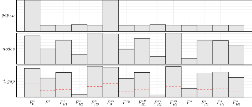
Figure 1: Comparative results for the proposed OWAP basic formulations applied to the Shortest Path Problem ($p=10$, $|V|=400$)

Inst			$F_{R2}^{z}$				$F_{R2}^{zy}$				$F^{s}$
$|V|$	$p$	$\alpha$	$t(\#)$	$t^{*}/gap^{*}$	$\#nodes$	$gap_{LR}$	$t(\#)$	$t^{*}/gap^{*}$	$\#nodes$	$gap_{LR}$	$t(\#)$	$t^{*}/gap^{*}$	$\#nodes$	$gap_{LR}$
100	4	0.4	0.5	0.6	15	55.79	0.4	0.6	13	55.79	8.4	59.9	16959	53.72
100	4	0.6	0.5	0.6	41	40.17	12	116.5	56370	40.17	31.9	213.4	113492	37.39
100	4	0.8	0.4	0.5	61	24.26	0.4	0.5	48	24.26	2.4	7.9	2871	20.79
100	7	0.4	0.6	0.7	200	52.77	0.6	0.8	177	52.77	121 (8)	40.66%	210086	51.11
100	7	0.6	0.7	0.8	360	38.19	0.8	1.6	468	38.19	121 (8)	22.74%	193167	36.01
100	7	0.8	0.9	1.6	839	23.76	0.9	1.4	760	23.76	20.8	125.9	36870	21.08
100	10	0.4	2.1	4.2	6658	51.98	2.5	10.3	9239	51.98	195.2 (7)	43.64%	273035	49.29
100	10	0.6	4.1	13.2	16386	37.89	2.8	11.1	9985	37.89	178.6 (8)	24.44%	238513	34.4
100	10	0.8	5.5	27.9	23353	24.83	13.1	49.4	57599	24.83	95.3	500.7	127230	20.61
225	4	0.4	0.8	1	48	55.77	0.8	1.1	45	55.77	64.4 (9)	52.43%	29874	55
225	4	0.6	0.8	1	44	39.42	0.8	1	49	39.42	91.5 (9)	31.77%	41747	38.31
225	4	0.8	0.8	1.1	95	22.13	0.8	1.2	84	22.13	243.8 (6)	14.08%	70842	20.7
225	7	0.4	1.2	1.3	99	52.61	1.3	1.8	151	52.61	129 (8)	49.52%	41763	51.29
225	7	0.6	3.3	8.8	1554	37.63	16.2	143.6	10871	37.63	185.6 (7)	31.25%	63146	35.83
225	7	0.8	4.6	22.1	3082	22.76	2.6	6.1	1204	22.76	305 (5)	14.19%	105127	20.44
225	10	0.4	9.1	62.7	6427	51.68	5.4	24.9	4222	51.68	317.1 (5)	49.98%	95076	50.33
225	10	0.6	15.2	56.6	10148	37.07	10.8	39.7	7537	37.07	319.5 (5)	32.14%	96370	35.15
225	10	0.8	38.1	147.8	41223	23.12	29.6	141.5	32090	23.12	279.6 (6)	15.16%	85419	20.81
400	4	0.4	1.4	1.8	57	55.07	1.3	1.6	55	55.07	3.3	16.8	286	54.44
400	4	0.6	1.6	2	95	38.71	1.5	1.8	76	38.71	88.5 (9)	35.79%	13806	37.84
400	4	0.8	1.8	2.9	182	21.57	1.8	3.1	265	21.57	255.9 (6)	17.21%	49806	20.47
400	7	0.4	6.5	41.1	1102	52.72	19.3	169	4370	52.72	76.4 (9)	50.67%	9192	51.85
400	7	0.6	9.4	62.6	2952	37.41	63.4 (9)	33.32%	10416	37.48	70.9 (9)	34.59%	8711	36.27
400	7	0.8	8.1	30.2	1994	21.87	7.2	24.6	1999	21.87	368.8 (4)	18.29%	32614	20.41
400	10	0.4	158.5 (9)	1.09%	100979	51.8	116.1	242.7	83991	51.8	306.4 (5)	48.93%	24184	50.73
400	10	0.6	61.8	121.5	37448	36.48	33.2	115.9	17308	36.48	132.4 (8)	31.48%	10395	35.01
400	10	0.8	229.9 (8)	0.61%	143034	21.82	155.6 (9)	0.04%	104042	21.82	142.6 (8)	17.18%	12829	19.99

Table 9: Results obtained for the three best OWAP basic formulations applied to the Shortest Path Problem

From the results displayed in Table 9 and Figure 1, we observe first that the $gap_{LR}$ is similar for all formulations except for $F_{0}^{z}$ and $F_{0}^{zy}$, where a 100% of gap is reached. Formulations $F_{R2}^{z}$ and $F_{R2}^{zy}$ increase slightly the $gap_{LR}$ in comparison with the remaining formulations but this does not affect negatively in the exploration as we see next. The values of $nodes$ and $t,gap$ are strongly related for each one of the formulations. $F_{0}^{z}$, $F_{R3}^{z}$, $F_{0}^{zy}$ and $F_{R3}^{zy}$ give the worst values. In contrast, $F_{R2}^{z}$, $F_{R2}^{zy}$ and $F^{s}$ produce the best values. In addition, we observe a regular behavior among all formulations with $s$ variables, namely $F^{s}$, $F_{R1}^{s}$, $F_{R2}^{s}$ and $F_{R3}^{s}$. Regarding to the PMP, analogous conclusions can be obtained in Table 10 and Figure 2 for the $gap_{LR}$ and the relations between $nodes$ and $t,gap$. However, in this case, formulations $F_{R1}^{z}$ and $F_{R1}^{zy}$ produce the best values together with $F_{R1}^{s}$, $F_{R2}^{s}$ and $F_{R3}^{s}$.

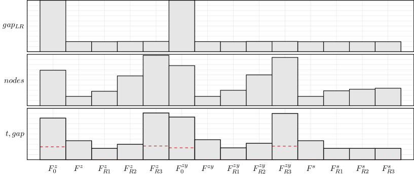
Figure 2: Comparative results for the proposed OWAP basic formulations applied to the Perfect Matching Problem ($p=10$, $|V|=400$)

Inst			$F_{R1}^{z}$				$F_{R1}^{zy}$				$F_{R1}^{s}$
$|V|$	$p$	$\alpha$	$t(\#)$	$t^{*}/gap^{*}$	$\#nodes$	$gap_{LR}$	$t(\#)$	$t^{*}/gap^{*}$	$\#nodes$	$gap_{LR}$	$t(\#)$	$t^{*}/gap^{*}$	$\#nodes$	$gap_{LR}$
100	4	0.4	0.6	0.7	186	55.44	0.6	0.7	139	55.44	0.5	0.7	147	55.44
100	4	0.6	0.6	0.7	152	38.98	0.6	0.7	140	38.98	0.6	0.8	175	38.98
100	4	0.8	0.6	0.7	302	21.53	0.7	0.8	329	21.53	0.6	0.7	157	21.53
100	7	0.4	1	1.3	236	52.18	1	1.2	256	52.18	1	1.2	205	52.18
100	7	0.6	1.1	1.4	480	35.97	1.2	1.8	591	35.97	1.2	1.6	529	35.97
100	7	0.8	1.4	2	965	20.27	1.5	2.3	1008	20.27	1.3	1.8	1075	20.27
100	10	0.4	1.5	1.9	299	50.66	1.7	4.1	580	50.66	1.5	1.9	333	50.66
100	10	0.6	1.9	2.6	963	34.85	1.9	2.9	985	34.85	2	2.8	922	34.85
100	10	0.8	6	19.4	6329	20.2	5.6	17.6	5364	20.2	6.1	19.8	7018	20.2
225	4	0.4	2.1	4.4	1188	55.09	2	2.9	990	55.09	1.9	4.1	1095	55.09
225	4	0.6	1.7	2.9	1236	38.57	1.7	2.5	1239	38.57	1.7	2.2	982	38.57
225	4	0.8	1.9	3.2	1101	21.09	1.9	3.7	1240	21.09	2	3.6	1221	21.09
225	7	0.4	7.1	22.8	9208	52.34	8.4	36	5617	52.34	8.7	29.3	6308	52.34
225	7	0.6	10	16	6038	36.27	9.7	18.3	6206	36.27	8.8	15.9	5432	36.27
225	7	0.8	17.2	62.5	10491	20.32	17.1	48.7	10746	20.32	14.7	50.1	9525	20.32
225	10	0.4	7.5	13.2	2136	50.25	7.4	12.4	2464	50.25	7.8	15.5	2265	50.25
225	10	0.6	32.4	123.2	15537	34.56	33.9	90.1	13763	34.56	31.5	70.1	15465	34.56
225	10	0.8	295 (8)	0.32%	114029	19.62	338.7 (7)	12.07%	130079	19.7	344.7 (8)	0.33%	133025	19.62
400	4	0.4	7.3	22.3	3345	55.37	6.3	15.5	2546	55.37	6.1	9.6	2777	55.37
400	4	0.6	6.7	11.9	4103	39.04	7.5	16.7	4044	39.04	8.7	25.3	6589	39.04
400	4	0.8	9	22.1	5397	21.03	11.4	44.9	6263	21.03	9.2	19.4	5194	21.03
400	7	0.4	34.4	144.4	10464	52.05	48.9	257	15696	52.05	37.7	218.2	11164	52.05
400	7	0.6	83.4	250.9	27604	36.12	74.5	209.5	26944	36.12	78.7	185.1	28692	36.12
400	7	0.8	84.4	187.6	28762	20.19	98.2	182.5	35369	20.19	92.6	206.4	34328	20.19
400	10	0.4	68.4	197.4	13777	50.58	86.7	387.2	17514	50.58	91.9	407.6	19024	50.58
400	10	0.6	289.4 (9)	0.11%	61886	34.54	335 (9)	0.24%	69457	34.54	285.7	563.5	59428	34.54
400	10	0.8	583.5 (1)	0.42%	97022	19.5	599 (1)	0.4%	93171	19.5	577 (1)	0.43%	97258	19.52

Table 10: Results obtained for the three best OWAP basic formulations applied to the Perfect Matching Problem

Figures 3 and 4 report analogous items as Figures 1 and 2, but now when the valid inequalities of Section 4 are incorporated to the best basic formulations obtained for each combinatorial object. The $x-$axis displays the different variations in the formulations, starting first with the best basic formulation. Next labels refer to the valid inequality that has been added. Labels of the valid inequalities correspond with those of Section 4, where “.1” and “.2” refer to the two inequalities displayed in a single equation (for example the two valid inequalities of equation (33) are labeled as (33.1) and (33.2)). In the following we will refer indistinctly to a valid inequality and the formulation that includes such valid inequality. All displayed bars represent percentages of mean values computed over 30 random instances with $p=10$, $|V|=400$ and $\alpha\in\{0.4,0.6,0.8\}$.

Figure 3: Comparative results for the proposed OWAP reinforced formulations applied to the Shortest Path Problem ($p=10$, $|V|=400$)

From the results displayed in Figure 3, we observe first that the $gap_{LR}$ is similar for all formulations but (34.1), (38.1), (39), (41.1) and (42). As compared with with $F_{R2}^{zy}$, formulation (38.1) improves the values of $gap_{LR}$, $nodes$ and $t,gap$. However, (34.1), (41.1) and (42) improve $gap_{LR}$ but are not able to improve $nodes$ or $t,gap$. We also note that (39) increases $gap_{LR}$ since this gap is computed with a (low quality) best solution found by the solver and the linear relaxation optima at the root node. In addition, formulations (33.1), (33.2) and (41.4) provide promising results in comparison with the values of $nodes$ and $t,gap$.

Figure 4: Comparative results for the proposed OWAP reinforced formulations applied to the Perfect Matching Problem ($p=10$, $|V|=400$)

From the results displayed in Figure 4, we observe first that the $gap_{LR}$ is similar for all formulations but (34.1), (38.1), (39) and (42). As compared with $F_{R1}^{z}$, formulations (34.1) and (38.1), improve $gap_{LR}$ and $nodes$ or $t,gap$. However, (42) improves $gap_{LR}$ but is not able to improve $nodes$ or $t,gap$ in comparison with the best basic formulation for PMP, namely $F_{R1}^{z}$. We also note that (39) increases $gap_{LR}$ since this gap is computed with a (low quality) best solution found by the solver and the linear relaxation optima at the root node. In addition, formulations (37.2), (38.2) and (41.3) provide promising results in comparison with the values of $nodes$ or $t,gap$.

In summary, we observe the performance of the OWAP formulation depends on its combination with the considered combinatorial object. In particular we conclude, from our computational experience, that for the SPP, it is convenient to apply $F^{zy}_{R2}$ reinforced with (33.1) and (33.2); although rather similar results can be obtained with $F^{z}_{R2}$. The conclusion for the PMP is different, because the best basic formulation is now $F^{z}_{R1}$ and the reinforcements (34.1). Once more, rather similar results are obtained for $F^{zy}_{R1}$ and $F^{s}_{R1}$. Therefore, we can not conclude whether there is a formulation superior to all the others regardless the domain $Q$ to be considered. For this reason it is important to have developed the catalogue of formulations and valid inequalities presented in this paper. In general, it is advisable to test them depending on the combinatorial object to be considered.

7 Appendix: Complete results obtained in the experiments

Inst			$F_{0}^{z}$				$F^{z}$				$F^{z}$′
$|V|$	$p$	$\alpha$	$t(\#)$	$t^{*}/gap^{*}$	$\#nodes$	$gap_{LR}$	$t(\#)$	$t^{*}/gap^{*}$	$\#nodes$	$gap_{LR}$	$t(\#)$	$t^{*}/gap^{*}$	$\#nodes$	$gap_{LR}$
100	4	0.4	61.9 (9)	41.15%	159186	100	2.2	12.3	2087	53.72	1.4	4.5	1005	53.72
100	4	0.6	1.6	2.5	2775	100	1.9	6.7	2149	37.39	17.1	117.1	72137	37.39
100	4	0.8	15.7	64	47308	100	8.9	38.9	15109	20.79	4.9	30.1	4885	20.79
100	7	0.4	539.6 (1)	55.52%	670773	100	73.8 (9)	38.38%	169704	51.11	114.9 (9)	40.83%	252250	51.11
100	7	0.6	599.2 (0)	42.4%	821449	100	71 (9)	19.84%	177585	36.01	62.1 (9)	16.07%	143671	36.01
100	7	0.8	599.2 (0)	30.88%	977772	100	21.8	96.5	45613	21.08	19.9	118	42932	21.08
100	10	0.4	599.2 (0)	59.33%	598177	100	181.6 (8)	38.78%	299151	49.29	186.8 (7)	40.11%	204286	49.29
100	10	0.6	599.4 (0)	47.99%	721323	100	131.6 (8)	22.48%	184532	34.4	192.6 (7)	23.86%	237500	34.43
100	10	0.8	599.5 (0)	36.12%	816612	100	70.2	479.4	101591	20.61	57.8	376.8	83723	20.61
225	4	0.4	4	11.5	1814	100	129.7 (8)	51.55%	48659	54.96	138.9 (8)	53.16%	52164	55.06
225	4	0.6	365 (6)	19.25%	308001	100	138.3 (8)	32.58%	47943	38.31	294.5 (6)	33.99%	133651	38.39
225	4	0.8	599.2 (0)	19.46%	405027	100	273 (7)	12.11%	130154	20.7	350.7 (5)	14.57%	130975	20.7
225	7	0.4	599.4 (0)	62.68%	216392	100	361.5 (4)	48.61%	181096	51.74	151.4 (9)	39.95%	58002	51.2
225	7	0.6	599.5 (0)	51.17%	253663	100	363.1 (4)	32.18%	176663	36.05	361 (4)	32.66%	146512	35.83
225	7	0.8	599.5 (0)	41.18%	265937	100	420.8 (3)	14.49%	221975	20.44	288.8 (6)	14.55%	133194	20.45
225	10	0.4	599.7 (0)	63.54%	166127	100	396.8 (4)	50.6%	118651	50.61	332.3 (5)	47.82%	92470	50.3
225	10	0.6	599.7 (0)	55.79%	208149	100	421.8 (3)	32.03%	125420	35.43	335.9 (5)	32.85%	111328	35.36
225	10	0.8	599.7 (0)	47.37%	227825	100	324.9 (5)	15.12%	97109	20.84	298.3 (6)	14.91%	109912	20.71
400	4	0.4	211.8 (7)	46.17%	44001	100	200.9 (7)	52.86%	32709	54.47	227.4 (7)	51.74%	43043	54.46
400	4	0.6	572.4 (1)	40.28%	123465	100	371.9 (4)	37.16%	51494	38.03	182.5 (8)	36.23%	31789	37.89
400	4	0.8	599.3 (0)	63.06%	146115	100	464.5 (3)	17.95%	72353	20.47	391.2 (5)	17.89%	64058	20.47
400	7	0.4	599.2 (0)	64.86%	78332	100	599.8 (0)	53.96%	85672	53.77	496.5 (2)	54.52%	51199	53.01
400	7	0.6	599.3 (0)	54.05%	97758	100	540.5 (1)	36.56%	77694	37.07	550.7 (1)	36.37%	53000	36.78
400	7	0.8	599.3 (0)	45.98%	106458	100	481.7 (2)	18.53%	70106	20.52	599.7 (0)	17.89%	59361	20.42
400	10	0.4	599.5 (0)	65.97%	59878	100	314.7 (5)	50.22%	22479	50.93	376.5 (4)	52.17%	23753	51.09
400	10	0.6	599.3 (0)	56.75%	82904	100	198.9 (7)	34.1%	14858	35.12	225.6 (7)	32.13%	18486	35.06
400	10	0.8	599.4 (0)	52.8%	82418	100	145.1 (8)	15.5%	11060	19.98	258.4 (6)	17.55%	21698	20.04

Table 11: Results obtained for OWAP formulations with the Shortest Path Problem

Inst			$F_{R1}^{z}$				$F_{R2}^{z}$				$F_{R3}^{z}$
$|V|$	$p$	$\alpha$	$t(\#)$	$t^{*}/gap^{*}$	$\#nodes$	$gap_{LR}$	$t(\#)$	$t^{*}/gap^{*}$	$\#nodes$	$gap_{LR}$	$t(\#)$	$t^{*}/gap^{*}$	$\#nodes$	$gap_{LR}$
100	4	0.4	4.5	17.9	7045	53.72	0.5	0.6	15	55.79	360.7 (4)	35.38%	1088918	53.72
100	4	0.6	8.4	43.7	20767	37.39	0.5	0.6	41	40.17	398.1 (4)	19.95%	940627	37.39
100	4	0.8	6.3	21.4	9361	20.79	0.4	0.5	61	24.26	28.1	84.1	73283	20.79
100	7	0.4	183.8 (7)	39.39%	505058	51.21	0.6	0.7	200	52.77	599.2 (0)	44.67%	1267412	51.52
100	7	0.6	177.4 (8)	22.51%	552821	36.01	0.7	0.8	360	38.19	599.2 (0)	28.4%	1451450	36.12
100	7	0.8	31.2	79	68528	21.08	0.9	1.6	839	23.76	494.3 (4)	6.67%	2046319	21.08
100	10	0.4	131 (8)	38.43%	211989	49.29	2.1	4.2	6658	51.98	560.6 (1)	47.89%	1405677	49.98
100	10	0.6	132.7 (8)	18.42%	360647	34.43	4.1	13.2	16386	37.89	599.4 (0)	29.69%	1566146	34.86
100	10	0.8	86.2	388.2	176071	20.61	5.5	27.9	23353	24.83	539.1 (2)	13.52%	1982531	20.61
225	4	0.4	128.9 (8)	52.67%	66387	55.01	0.8	1	48	55.77	599.4 (0)	52.65%	346252	55.09
225	4	0.6	308.3 (5)	33.54%	154345	38.39	0.8	1	44	39.42	360 (4)	34.52%	207131	38.34
225	4	0.8	361.9 (5)	15.51%	140540	20.7	0.8	1.1	95	22.13	439.3 (4)	15.58%	206648	20.7
225	7	0.4	314.6 (5)	49.58%	160573	51.65	1.2	1.3	99	52.61	599.6 (0)	50.61%	312524	52.1
225	7	0.6	441.4 (3)	32.37%	233819	35.92	3.3	8.8	1554	37.63	599.7 (0)	32.98%	336958	36.43
225	7	0.8	526.7 (2)	13.95%	308827	20.44	4.6	22.1	3082	22.76	599.7 (0)	14.79%	307722	20.44
225	10	0.4	554.5 (1)	50.01%	270862	51.07	9.1	62.7	6427	51.68	599.7 (0)	51.52%	331748	52.53
225	10	0.6	599.8 (0)	31.67%	337820	35.75	15.2	56.6	10148	37.07	599.8 (0)	33.34%	334555	36.52
225	10	0.8	599.7 (0)	14.51%	279970	20.69	38.1	147.8	41223	23.12	599.7 (0)	16.15%	345339	20.85
400	4	0.4	195.8 (7)	52.37%	33251	54.44	1.4	1.8	57	55.07	599.7 (0)	54.69%	118795	54.6
400	4	0.6	325 (5)	35.5%	71726	38.01	1.6	2	95	38.71	539.9 (1)	36.64%	111458	38.04
400	4	0.8	367.4 (4)	17.8%	43381	20.47	1.8	2.9	182	21.57	599.8 (0)	18.03%	102960	20.47
400	7	0.4	541.2 (1)	54.39%	74342	53.16	6.5	41.1	1102	52.72	599.7 (0)	53.57%	121813	52.76
400	7	0.6	541.6 (1)	35.17%	92740	36.53	9.4	62.6	2952	37.41	599.7 (0)	36.68%	132839	36.89
400	7	0.8	544.3 (1)	17.86%	106851	20.4	8.1	30.2	1994	21.87	599.7 (0)	18.53%	110457	20.57
400	10	0.4	531.6 (2)	53.98%	89609	52.43	158.5 (9)	1.09%	100979	51.8	599.7 (0)	54.33%	101358	53.88
400	10	0.6	599.7 (0)	35.53%	84013	36.4	61.8	121.5	37448	36.48	599.7 (0)	36.05%	129485	36.6
400	10	0.8	599.7 (0)	17.75%	96917	20.25	229.9 (8)	0.61%	143034	21.82	599.7 (0)	17.86%	111753	20.2

Table 12: Results obtained for the OWAP formulations with the Shortest Path Problem

Inst			$F_{0}^{zy}$				$F^{zy}$				$F^{zy}$′
$|V|$	$p$	$\alpha$	$t(\#)$	$t^{*}/gap^{*}$	$\#nodes$	$gap_{LR}$	$t(\#)$	$t^{*}/gap^{*}$	$\#nodes$	$gap_{LR}$	$t(\#)$	$t^{*}/gap^{*}$	$\#nodes$	$gap_{LR}$
100	4	0.4	1.2	3.1	1192	100	121.2 (8)	31.45%	451392	53.72	85 (9)	33.02%	416097	53.72
100	4	0.6	2.9	9.1	5786	100	15.1	104.1	29720	37.39	4.4	25.5	7032	37.39
100	4	0.8	14.9	29.7	43225	100	5.7	22.2	8568	20.79	4.4	25	4359	20.79
100	7	0.4	599.1 (0)	56.76%	777811	100	82.3 (9)	35.05%	196817	51.11	121.8 (8)	33.93%	232458	51.19
100	7	0.6	599.1 (0)	44.1%	815725	100	63.6 (9)	8.86%	165583	36.01	67.9 (9)	18.4%	97103	36.01
100	7	0.8	599.2 (0)	26.56%	992683	100	20.2	107.4	42676	21.08	11.8	53.3	18601	21.08
100	10	0.4	599.3 (0)	59.5%	584890	100	132.3 (8)	42.34%	220685	49.29	187.6 (7)	38.16%	228058	49.29
100	10	0.6	599.4 (0)	47.08%	698012	100	176.2 (8)	23.12%	325255	34.4	184.5 (7)	24.44%	158769	34.4
100	10	0.8	599.5 (0)	37.21%	832031	100	83.1	260.9	118290	20.61	122.9	499.5	148775	20.61
225	4	0.4	42.7	293.1	26879	100	129.8 (8)	49.74%	57642	55.01	285.9 (6)	52.02%	123411	54.97
225	4	0.6	404.3 (5)	17.48%	335937	100	185.7 (7)	31.19%	99753	38.36	362.6 (4)	34.45%	160383	38.39
225	4	0.8	599.7 (0)	14.1%	436690	100	327.3 (5)	14.76%	103352	20.7	540.4 (1)	14.31%	223399	20.7
225	7	0.4	599.9 (0)	61.69%	216243	100	480.2 (2)	50.43%	227345	51.59	374.2 (4)	51.31%	135242	51.69
225	7	0.6	599.5 (0)	57.25%	248810	100	420.6 (3)	32.51%	210813	35.87	448.8 (3)	33.08%	152915	35.89
225	7	0.8	599.9 (0)	51.27%	275751	100	307.1 (5)	14.84%	151530	20.45	529.6 (3)	15.35%	205445	20.56
225	10	0.4	599.8 (0)	64.4%	165068	100	421.5 (3)	49.78%	121243	50.58	311.9 (5)	47.81%	87477	50.36
225	10	0.6	599.9 (0)	64.91%	211343	100	311.6 (5)	31.66%	93967	35.35	303.6 (5)	32.22%	89976	35.68
225	10	0.8	600 (0)	47.48%	215323	100	247.5 (6)	15.04%	73111	20.71	321.3 (5)	15.62%	89902	20.73
400	4	0.4	361.2 (4)	49.35%	82543	100	153 (8)	52.96%	27764	54.44	100.9 (9)	53.09%	19609	54.44
400	4	0.6	598 (1)	38.99%	145270	100	298.6 (6)	36.15%	56477	37.91	371.1 (4)	36.31%	51542	38.01
400	4	0.8	599.8 (0)	34.48%	131878	100	425.9 (3)	17.52%	63344	20.47	432.6 (3)	18.51%	49572	20.47
400	7	0.4	599.8 (0)	64.49%	78184	100	481 (2)	52.37%	68194	53.06	563.9 (1)	53.36%	55424	53.02
400	7	0.6	599.8 (0)	53.68%	96075	100	540.4 (1)	36.55%	76295	37.16	540.3 (1)	36.44%	44656	36.82
400	7	0.8	599.8 (0)	42.76%	108088	100	481.8 (2)	18.09%	71226	20.37	450.8 (3)	18.24%	68513	20.4
400	10	0.4	599.7 (0)	66.58%	58295	100	371.3 (4)	50.51%	29467	50.99	371.6 (5)	50.67%	24697	50.84
400	10	0.6	599.7 (0)	56.48%	83222	100	252.2 (6)	33.31%	20435	35.04	278.1 (6)	33.63%	23601	35.2
400	10	0.8	599.7 (0)	49.98%	84953	100	259.4 (6)	16.84%	21451	19.99	148.3 (8)	17.27%	11315	20.03

Table 13: Results obtained for the OWAP formulations with the Shortest Path Problem

Inst			$F_{R1}^{zy}$				$F_{R2}^{zy}$				$F_{R3}^{zy}$
$|V|$	$p$	$\alpha$	$t(\#)$	$t^{*}/gap^{*}$	$\#nodes$	$gap_{LR}$	$t(\#)$	$t^{*}/gap^{*}$	$\#nodes$	$gap_{LR}$	$t(\#)$	$t^{*}/gap^{*}$	$\#nodes$	$gap_{LR}$
100	4	0.4	65.6 (9)	23.26%	241924	53.72	0.4	0.6	13	55.79	322 (5)	42.47%	845867	53.72
100	4	0.6	7.5	40.8	15505	37.39	12	116.5	56370	40.17	241.6 (8)	19.94%	672083	37.39
100	4	0.8	8.3	25.4	14166	20.79	0.4	0.5	48	24.26	42.5	246.4	113968	20.79
100	7	0.4	315.7 (5)	43.06%	656760	51.11	0.6	0.8	177	52.77	599.5 (0)	44.43%	1266772	51.11
100	7	0.6	184 (7)	21.71%	362904	36.02	0.8	1.6	468	38.19	599.3 (0)	28.49%	1362716	36.19
100	7	0.8	28.7	61.1	64042	21.08	0.9	1.4	760	23.76	491.4 (3)	6.46%	2116465	21.08
100	10	0.4	165.3 (8)	39.18%	309014	49.29	2.5	10.3	9239	51.98	599.4 (0)	44.7%	1410323	49.62
100	10	0.6	106.9 (9)	15.18%	257461	34.4	2.8	11.1	9985	37.89	599.1 (0)	29.21%	1489995	34.7
100	10	0.8	59.3	290.2	117576	20.61	13.1	49.4	57599	24.83	558.7 (1)	11.48%	2253482	20.64
225	4	0.4	86 (9)	48.2%	39407	54.96	0.8	1.1	45	55.77	599.4 (0)	51.97%	300625	55.09
225	4	0.6	203.6 (7)	33.71%	107278	38.34	0.8	1	49	39.42	479.5 (2)	32.79%	244773	38.31
225	4	0.8	309.9 (5)	14.89%	99639	20.7	0.8	1.2	84	22.13	471.1 (3)	15.78%	194755	20.7
225	7	0.4	427.2 (3)	49.21%	226670	51.59	1.3	1.8	151	52.61	599.6 (0)	50.54%	316386	52.35
225	7	0.6	484.1 (2)	32.39%	250074	35.92	16.2	143.6	10871	37.63	599.6 (0)	32.92%	332670	36.32
225	7	0.8	551.3 (1)	13.9%	272995	20.44	2.6	6.1	1204	22.76	539.7 (1)	15.18%	303691	20.45
225	10	0.4	599.6 (0)	48.93%	308090	50.64	5.4	24.9	4222	51.68	599.6 (0)	51.96%	325027	52.86
225	10	0.6	580.6 (1)	31.75%	307517	35.6	10.8	39.7	7537	37.07	599.9 (0)	33.36%	385794	36.12
225	10	0.8	600 (0)	14.4%	298384	20.73	29.6	141.5	32090	23.12	599.7 (0)	16.66%	346034	20.84
400	4	0.4	208.6 (7)	51.54%	44423	54.44	1.3	1.6	55	55.07	541 (1)	52.68%	102735	54.44
400	4	0.6	372.1 (4)	37.31%	66668	37.97	1.5	1.8	76	38.71	541 (1)	35.41%	112968	38.03
400	4	0.8	288.8 (6)	18.01%	44492	20.47	1.8	3.1	265	21.57	599.6 (0)	17.94%	125836	20.47
400	7	0.4	599.7 (0)	54.35%	106106	53.05	19.3	169	4370	52.72	599.8 (0)	55.43%	108756	54.22
400	7	0.6	509.6 (2)	35.93%	81877	37.05	63.4 (9)	33.32%	10416	37.48	599.6 (0)	35.83%	116993	37.01
400	7	0.8	544.1 (1)	18.44%	105707	20.6	7.2	24.6	1999	21.87	599.7 (0)	18%	122164	20.61
400	10	0.4	599.8 (0)	53.58%	102856	52.38	116.1	242.7	83991	51.8	599.7 (0)	54.19%	122568	53.59
400	10	0.6	529.3 (2)	36.02%	72585	36.14	33.2	115.9	17308	36.48	599.8 (0)	35.96%	117557	36.53
400	10	0.8	599.7 (0)	17.61%	115177	20.27	155.6 (9)	0.04%	104042	21.82	599.7 (0)	18.17%	79055	20.26

Table 14: Results obtained for the OWAP formulations with the Shortest Path Problem

Inst			$F^{s}$				$F_{R1}^{s}$				$F_{R2}^{s}$
$|V|$	$p$	$\alpha$	$t(\#)$	$t^{*}/gap^{*}$	$\#nodes$	$gap_{LR}$	$t(\#)$	$t^{*}/gap^{*}$	$\#nodes$	$gap_{LR}$	$t(\#)$	$t^{*}/gap^{*}$	$\#nodes$	$gap_{LR}$
100	4	0.4	8.4	59.9	16959	53.72	66.4 (9)	27.51%	204809	53.72	16.9	114.5	40710	53.72
100	4	0.6	31.9	213.4	113492	37.39	72.3	460.2	275423	37.39	4.3	17	6899	37.39
100	4	0.8	2.4	7.9	2871	20.79	8.3	23.2	11449	20.79	8.5	20.9	14436	20.79
100	7	0.4	121 (8)	40.66%	210086	51.11	124.2 (8)	11.44%	492697	51.11	63.5 (9)	43.15%	102947	51.11
100	7	0.6	121 (8)	22.74%	193167	36.01	185.7 (7)	23.17%	477873	36.01	11.2	50.4	28267	36.01
100	7	0.8	20.8	125.9	36870	21.08	38.8	105.4	94229	21.08	26.5	65.1	62967	21.08
100	10	0.4	195.2 (7)	43.64%	273035	49.29	75.8 (9)	22%	172053	49.29	20	121.2	50657	49.29
100	10	0.6	178.6 (8)	24.44%	238513	34.4	108.7 (9)	7.87%	322084	34.4	151.2 (8)	23.02%	303828	34.4
100	10	0.8	95.3	500.7	127230	20.61	63.7	298.7	132170	20.61	57.4	201.2	132973	20.61
225	4	0.4	64.4 (9)	52.43%	29874	55	72.6 (9)	49.94%	34891	55.04	198.3 (7)	52.09%	104058	55.08
225	4	0.6	91.5 (9)	31.77%	41747	38.31	140.4 (9)	30.08%	75346	38.31	304 (5)	31.95%	149300	38.31
225	4	0.8	243.8 (6)	14.08%	70842	20.7	257.8 (7)	13.65%	123343	20.7	437 (4)	14.76%	178778	20.7
225	7	0.4	129 (8)	49.52%	41763	51.29	313.3 (5)	50.41%	159171	51.38	489.8 (2)	49.98%	232281	51.73
225	7	0.6	185.6 (7)	31.25%	63146	35.83	265.6 (6)	31.59%	154086	35.76	472.1 (3)	32.27%	269321	36.02
225	7	0.8	305 (5)	14.19%	105127	20.44	562.7 (3)	14.08%	385137	20.44	577.7 (1)	13.89%	353657	20.44
225	10	0.4	317.1 (5)	49.98%	95076	50.33	599.5 (0)	49.77%	270100	51.61	599.4 (0)	51.24%	286845	51.72
225	10	0.6	319.5 (5)	32.14%	96370	35.15	565.7 (1)	31.87%	268250	35.64	599.7 (0)	31.65%	270293	35.8
225	10	0.8	279.6 (6)	15.16%	85419	20.81	599.3 (0)	14.71%	305531	20.9	599.5 (0)	14.01%	292841	20.79
400	4	0.4	3.3	16.8	286	54.44	253.7 (6)	55.16%	36622	54.6	311 (5)	54.17%	51331	54.76
400	4	0.6	88.5 (9)	35.79%	13806	37.84	355 (5)	36.67%	68752	37.93	258.4 (6)	35.91%	48491	37.92
400	4	0.8	255.9 (6)	17.21%	49806	20.47	226.7 (7)	18.11%	25218	20.47	374.7 (4)	17.85%	41044	20.47
400	7	0.4	76.4 (9)	50.67%	9192	51.85	546 (1)	54.01%	100473	52.97	497.6 (2)	52.93%	92358	52.81
400	7	0.6	70.9 (9)	34.59%	8711	36.27	599.6 (0)	36.56%	97419	36.79	490.8 (2)	36.45%	76146	36.92
400	7	0.8	368.8 (4)	18.29%	32614	20.41	485.1 (2)	17.99%	69436	20.71	599.3 (0)	18.38%	81188	20.57
400	10	0.4	306.4 (5)	48.93%	24184	50.73	508.1 (2)	52.44%	79421	52.03	599.6 (0)	54.16%	89357	53.69
400	10	0.6	132.4 (8)	31.48%	10395	35.01	599.4 (0)	33.61%	117393	35.56	599.6 (0)	34.98%	98170	36.4
400	10	0.8	142.6 (8)	17.18%	12829	19.99	599.4 (0)	17.64%	80443	20.29	599.4 (0)	17.58%	109094	20.18

Table 15: Results obtained for the OWAP formulations with the Shortest Path Problem

Inst			$F_{R3}^{s}$
$|V|$	$p$	$\alpha$	$t(\#)$	$t^{*}/gap^{*}$	$\#nodes$	$gap_{LR}$
100	4	0.4	91.2	402.2	384235	53.72
100	4	0.6	53.7	296.4	220361	37.39
100	4	0.8	3.3	13.2	3412	20.79
100	7	0.4	66.8 (9)	32.13%	184653	51.11
100	7	0.6	62.4 (9)	16.05%	177939	36.01
100	7	0.8	4.8	25	8846	21.08
100	10	0.4	123.6 (8)	39.94%	219511	49.29
100	10	0.6	121.9 (8)	15.68%	371819	34.4
100	10	0.8	4.6	9.6	7553	20.61
225	4	0.4	190.2 (7)	51.96%	91128	54.97
225	4	0.6	127.4 (8)	33.79%	71841	38.41
225	4	0.8	245.5 (6)	14.16%	78074	20.7
225	7	0.4	313.7 (5)	50.43%	151042	51.36
225	7	0.6	563.6 (1)	32.75%	279849	36.07
225	7	0.8	449.7 (3)	14.28%	223068	20.44
225	10	0.4	293.5 (6)	49.76%	134368	50.53
225	10	0.6	489.2 (2)	32.65%	219326	35.92
225	10	0.8	338 (5)	14.78%	162308	20.73
400	4	0.4	132.2 (8)	52.61%	29642	54.47
400	4	0.6	277.2 (6)	35.79%	57596	37.98
400	4	0.8	423.8 (3)	18.1%	69373	20.47
400	7	0.4	357 (5)	52.98%	58912	52.73
400	7	0.6	357.2 (5)	35.86%	56379	36.64
400	7	0.8	435.6 (3)	18.38%	64149	20.33
400	10	0.4	559.4 (1)	53.23%	88799	52.39
400	10	0.6	446.1 (3)	34.22%	53445	35.83
400	10	0.8	386.7 (4)	17.59%	48957	20.16

Table 16: Results obtained for the OWAP formulations with the Shortest Path Problem

Inst			$F_{0}^{z}$				$F^{z}$				$F^{z}$′
$|V|$	$p$	$\alpha$	$t(\#)$	$t^{*}/gap^{*}$	$\#nodes$	$gap_{LR}$	$t(\#)$	$t^{*}/gap^{*}$	$\#nodes$	$gap_{LR}$	$t(\#)$	$t^{*}/gap^{*}$	$\#nodes$	$gap_{LR}$
100	4	0.4	1.3	1.6	694	100	0.7	1	109	55.44	0.8	1	137	55.44
100	4	0.6	132.1	570.7	395386	100	0.7	1	196	38.98	0.7	0.9	136	38.98
100	4	0.8	65.2	363.1	174806	100	0.8	1	235	21.53	0.8	1.3	244	21.53
100	7	0.4	164.1 (8)	15.52%	237915	100	2.4	3.5	405	52.18	1.6	2.1	218	52.18
100	7	0.6	445.1 (5)	24.15%	438889	100	2.3	3	452	35.97	1.7	2.2	383	35.97
100	7	0.8	599.3 (0)	38.43%	473919	100	3.3	5.3	1302	20.27	2.2	3	925	20.27
100	10	0.4	569.9 (1)	24.29%	267816	100	5.3	6.9	485	50.66	2.9	4.3	284	50.66
100	10	0.6	599.3 (0)	13%	248655	100	7.5	11.7	1162	34.85	4.1	5.7	1001	34.85
100	10	0.8	599.4 (0)	40.14%	229928	100	21.2	61.7	5799	20.2	14.4	48.2	6302	20.2
225	4	0.4	133.1 (8)	22.67%	196711	100	2.6	4.4	977	55.09	2.7	5.3	1339	55.09
225	4	0.6	169.1 (8)	24.65%	159699	100	2.4	3.7	1156	38.57	2.4	3.1	1148	38.57
225	4	0.8	151.7 (8)	12.9%	115889	100	2.6	3.8	1432	21.09	2.6	5.7	1064	21.09
225	7	0.4	599.4 (0)	26.96%	164416	100	21	62.4	9718	52.34	15.4	54.9	5102	52.34
225	7	0.6	599.3 (0)	12.26%	148547	100	34.1	126.8	12967	36.27	19.3	28.5	5883	36.27
225	7	0.8	599.3 (0)	21.17%	126129	100	47	169.8	12076	20.32	30	117.5	10155	20.32
225	10	0.4	599.3 (0)	35.34%	97866	100	26.8	51.9	2100	50.25	19.3	33.7	2101	50.25
225	10	0.6	599.7 (0)	43.06%	72292	100	179.4 (9)	20.95%	16700	34.68	98.6	339.8	15018	34.56
225	10	0.8	599.5 (0)	48.17%	63656	100	596.9 (1)	0.61%	58769	19.64	516 (3)	0.45%	70215	19.63
400	4	0.4	149.6 (9)	2.99%	70585	100	10.7	30.5	2933	55.37	8.7	16.9	2966	55.37
400	4	0.6	361.2 (6)	23.07%	144951	100	10.9	15.7	4019	39.04	10.8	24.4	5798	39.04
400	4	0.8	274.6 (8)	15.16%	96947	100	12.2	19.6	4720	21.03	14.4	29.4	7329	21.03
400	7	0.4	599.8 (0)	10.76%	65411	100	125.3 (9)	0.1%	14707	52.05	84.3	409.6	12412	52.05
400	7	0.6	599.9 (0)	39.05%	66520	100	224.5	397.9	31091	36.12	190.2	467.7	34097	36.12
400	7	0.8	599.9 (0)	47.19%	60028	100	223.7	575.4	35131	20.19	205	502.3	38941	20.19
400	10	0.4	599.8 (0)	67.35%	44020	100	301.3 (9)	0.53%	15116	50.59	168 (9)	0.3%	12093	50.59
400	10	0.6	599.8 (0)	63.84%	36930	100	511 (2)	0.55%	22643	34.58	471.8 (5)	0.26%	31918	34.54
400	10	0.8	599.8 (0)	67.82%	32663	100	599.9 (0)	0.63%	36012	19.59	599.8 (0)	0.42%	33206	19.53

Table 17: Results obtained for the OWAP formulations with the Perfect Matching Problem

Inst			$F_{R1}^{z}$				$F_{R2}^{z}$				$F_{R3}^{z}$
$|V|$	$p$	$\alpha$	$t(\#)$	$t^{*}/gap^{*}$	$\#nodes$	$gap_{LR}$	$t(\#)$	$t^{*}/gap^{*}$	$\#nodes$	$gap_{LR}$	$t(\#)$	$t^{*}/gap^{*}$	$\#nodes$	$gap_{LR}$
100	4	0.4	0.6	0.7	186	55.44	0.7	0.8	138	55.98	212.2 (7)	19.55%	628046	55.44
100	4	0.6	0.6	0.7	152	38.98	0.6	0.6	149	39.71	130.2 (8)	13.38%	354878	38.98
100	4	0.8	0.6	0.7	302	21.53	0.6	0.8	234	22.47	164.1 (8)	5.69%	487138	21.53
100	7	0.4	1	1.3	236	52.18	1.2	1.5	1020	53.23	599.3 (0)	46.18%	590657	52.19
100	7	0.6	1.1	1.4	480	35.97	60.9 (9)	13.62%	99261	37.43	599.3 (0)	31.27%	662540	35.97
100	7	0.8	1.4	2	965	20.27	1.6	3.1	1419	22.02	599.3 (0)	16.8%	880878	20.3
100	10	0.4	1.5	1.9	299	50.66	7.4	28.9	22875	51.75	599.3 (0)	46.74%	339601	50.83
100	10	0.6	1.9	2.6	963	34.85	2.6	4.5	2032	36.29	599.3 (0)	32.35%	392747	35.35
100	10	0.8	6	19.4	6329	20.2	11.3	36.2	13433	21.97	599.3 (0)	18.05%	730420	20.56
225	4	0.4	2.1	4.4	1188	55.09	1.9	3	1003	55.48	286.9 (6)	44.05%	212277	55.3
225	4	0.6	1.7	2.9	1236	38.57	1.7	2.5	1262	39.1	193.8 (8)	22.64%	157652	38.57
225	4	0.8	1.9	3.2	1101	21.09	2.1	3.8	1504	21.77	436.6 (3)	13.99%	357325	21.09
225	7	0.4	7.1	22.8	9208	52.34	17.9	96.4	21252	52.73	599.3 (0)	48.08%	176693	52.59
225	7	0.6	10	16	6038	36.27	12.3	33.5	8888	36.79	599.3 (0)	32.95%	191613	36.45
225	7	0.8	17.2	62.5	10491	20.32	17.6	67.6	11652	20.97	599.3 (0)	17.7%	232228	20.43
225	10	0.4	7.5	13.2	2136	50.25	18.7	59.6	15457	50.65	599.3 (0)	48.46%	102767	50.7
225	10	0.6	32.4	123.2	15537	34.56	45.3	101.4	27800	35.09	599.3 (0)	33.15%	139120	35.01
225	10	0.8	295 (8)	0.32%	114029	19.62	402.6 (6)	0.31%	169450	20.26	599.3 (0)	18.82%	164745	19.95
400	4	0.4	7.3	22.3	3345	55.37	6.5	17	3311	55.5	455.6 (5)	45.64%	119265	55.4
400	4	0.6	6.7	11.9	4103	39.04	8.6	27.3	6816	39.2	360.4 (7)	31.89%	99906	39.06
400	4	0.8	9	22.1	5397	21.03	12.1	25.5	8260	21.24	512.7 (2)	16.34%	187051	21.03
400	7	0.4	34.4	144.4	10464	52.05	53.4	111.5	23341	52.26	599.9 (0)	48.8%	85058	52.56
400	7	0.6	83.4	250.9	27604	36.12	112.2	240.7	42546	36.4	599.9 (0)	33.56%	93893	36.6
400	7	0.8	84.4	187.6	28762	20.19	224.3 (9)	0.44%	146178	20.55	599.9 (0)	18.1%	118886	20.38
400	10	0.4	68.4	197.4	13777	50.58	278.2 (7)	0.45%	104776	50.79	599.8 (0)	49.31%	53902	51.49
400	10	0.6	289.4 (9)	0.11%	61886	34.54	338.6 (8)	0.19%	81662	34.8	599.9 (0)	33.99%	59623	35.36
400	10	0.8	583.5 (1)	0.42%	97022	19.5	599.9 (0)	0.48%	108421	19.85	599.9 (0)	18.46%	66410	19.96

Table 18: Results obtained for the OWAP formulations with the Perfect Matching Problem

Inst			$F_{0}^{zy}$				$F^{zy}$				$F^{zy}$′
$|V|$	$p$	$\alpha$	$t(\#)$	$t^{*}/gap^{*}$	$\#nodes$	$gap_{LR}$	$t(\#)$	$t^{*}/gap^{*}$	$\#nodes$	$gap_{LR}$	$t(\#)$	$t^{*}/gap^{*}$	$\#nodes$	$gap_{LR}$
100	4	0.4	1.5	2.7	1346	100	0.8	1	162	55.44	0.7	0.9	109	55.44
100	4	0.6	19.2	93.3	48335	100	0.7	1	121	38.98	0.7	0.8	151	38.98
100	4	0.8	52.6	440.5	133230	100	0.8	1	229	21.53	0.7	1	197	21.53
100	7	0.4	70.2	271.4	74398	100	2.4	3.5	326	52.18	1.9	2.7	230	52.18
100	7	0.6	323.9 (7)	2.62%	311151	100	2.5	3.4	892	35.97	1.9	2.5	403	35.97
100	7	0.8	557.8 (1)	35.79%	458556	100	3.8	6.7	1540	20.27	2.7	4	892	20.27
100	10	0.4	557 (1)	24.67%	284261	100	4.8	6	448	50.66	4.6	6.9	417	50.66
100	10	0.6	599.3 (0)	11.6%	240287	100	6.7	8.9	1162	34.85	5.3	7.6	837	34.85
100	10	0.8	599.4 (0)	41%	223345	100	25.3	85.7	7395	20.2	18.1	45.9	6194	20.2
225	4	0.4	154.4 (8)	12.71%	121716	100	2.7	6.6	1576	55.09	2.4	3.4	965	55.09
225	4	0.6	250.2 (6)	12.41%	208907	100	2.3	3.4	1187	38.57	2.3	3.9	1118	38.57
225	4	0.8	120 (9)	9.23%	94574	100	2.5	4.6	1317	21.09	2.3	4.2	1056	21.09
225	7	0.4	532.5 (2)	3.39%	148297	100	19.1	58.9	7577	52.34	22.6	96.9	6535	52.34
225	7	0.6	599.3 (0)	40.02%	169446	100	23.7	43.5	6293	36.27	26.5	57.7	6779	36.27
225	7	0.8	599.3 (0)	46.4%	128394	100	43.4	167.1	12348	20.32	38	151	9632	20.32
225	10	0.4	599.5 (0)	34.2%	91387	100	26.5	61.8	2006	50.25	24	37.9	1866	50.25
225	10	0.6	599.6 (0)	39.98%	77386	100	130	362.9	18614	34.56	123.3	415	13898	34.56
225	10	0.8	599.8 (0)	57.06%	63465	100	588.8 (1)	0.51%	53502	19.63	576.1 (2)	0.52%	56654	19.63
400	4	0.4	285.4 (6)	5.64%	161874	100	12.2	37.6	3617	55.37	9.1	15.4	3329	55.37
400	4	0.6	231.2 (8)	11.41%	94521	100	14.4	29.8	5798	39.04	10.3	23	4340	39.04
400	4	0.8	384.6 (7)	16.27%	129285	100	13.9	33.8	5320	21.03	12.5	25.2	5468	21.03
400	7	0.4	599.9 (0)	31.44%	64070	100	128.6 (9)	0.23%	14895	52.05	104.5	383	13188	52.05
400	7	0.6	599.9 (0)	36.91%	63436	100	258.9	459.9	37140	36.12	205 (9)	0.05%	33027	36.12
400	7	0.8	599.8 (0)	48.62%	67620	100	267.4	526.6	39724	20.19	221.6	447.7	33662	20.19
400	10	0.4	599.9 (0)	37.68%	40006	100	253.7 (9)	0.26%	13493	50.59	252.2 (9)	0.31%	13052	50.59
400	10	0.6	599.9 (0)	42.48%	42371	100	558 (1)	0.39%	22812	34.57	488.3 (4)	0.35%	22428	34.56
400	10	0.8	599.8 (0)	63%	37416	100	599.8 (0)	0.59%	21413	19.58	599.9 (0)	0.49%	24123	19.53

Table 19: Results obtained for the OWAP formulations with the Perfect Matching Problem

Inst			$F_{R1}^{zy}$				$F_{R2}^{zy}$				$F_{R3}^{zy}$
$|V|$	$p$	$\alpha$	$t(\#)$	$t^{*}/gap^{*}$	$\#nodes$	$gap_{LR}$	$t(\#)$	$t^{*}/gap^{*}$	$\#nodes$	$gap_{LR}$	$t(\#)$	$t^{*}/gap^{*}$	$\#nodes$	$gap_{LR}$
100	4	0.4	0.6	0.7	139	55.44	0.7	0.8	133	55.98	189.7 (7)	22.3%	505255	55.47
100	4	0.6	0.6	0.7	140	38.98	0.6	0.7	147	39.71	29.5	160.6	91753	38.98
100	4	0.8	0.7	0.8	329	21.53	0.6	0.8	285	22.47	238.3 (7)	5.76%	703988	21.53
100	7	0.4	1	1.2	256	52.18	1.2	1.8	959	53.23	599.3 (0)	46.34%	605536	52.21
100	7	0.6	1.2	1.8	591	35.97	1.1	1.2	442	37.38	599.2 (0)	31.25%	677159	36.12
100	7	0.8	1.5	2.3	1008	20.27	1.5	2.4	1287	22.02	599.2 (0)	16.78%	911147	20.27
100	10	0.4	1.7	4.1	580	50.66	12.3	54.3	36234	51.75	599.2 (0)	46.81%	352950	50.83
100	10	0.6	1.9	2.9	985	34.85	3.9	16.7	5175	36.29	599.2 (0)	31.96%	407864	35.23
100	10	0.8	5.6	17.6	5364	20.2	29.4	183	42168	21.97	599.2 (0)	18.22%	844424	20.77
225	4	0.4	2	2.9	990	55.09	1.9	3.3	991	55.48	433.8 (4)	36.25%	332362	55.11
225	4	0.6	1.7	2.5	1239	38.57	4.6	29.6	7582	39.1	112.7 (9)	19.79%	81949	38.57
225	4	0.8	1.9	3.7	1240	21.09	1.9	3.2	1408	21.77	384.2 (4)	10.46%	335049	21.09
225	7	0.4	8.4	36	5617	52.34	15.1	48.9	16006	52.73	599.3 (0)	47.91%	180294	52.49
225	7	0.6	9.7	18.3	6206	36.27	9.8	19.9	6317	36.79	599.2 (0)	32.65%	201172	36.52
225	7	0.8	17.1	48.7	10746	20.32	28.6	172.6	20230	20.97	599.3 (0)	17.63%	217743	20.38
225	10	0.4	7.4	12.4	2464	50.25	116.1 (9)	0.11%	126039	50.65	599.2 (0)	48.35%	105064	50.73
225	10	0.6	33.9	90.1	13763	34.56	70.4	218.1	50035	35.09	599.3 (0)	33.24%	127851	35.03
225	10	0.8	338.7 (7)	12.07%	130079	19.7	367.3 (7)	0.33%	198458	20.27	599.4 (0)	18.61%	171503	20.08
400	4	0.4	6.3	15.5	2546	55.37	6.8	17.7	3494	55.5	382 (7)	47.5%	94550	55.42
400	4	0.6	7.5	16.7	4044	39.04	8.6	14.1	7036	39.2	422 (5)	32.69%	121143	39.08
400	4	0.8	11.4	44.9	6263	21.03	14.1	31	10928	21.24	475.2 (3)	15.57%	167062	21.03
400	7	0.4	48.9	257	15696	52.05	65.9	155.3	29514	52.26	599.8 (0)	49.42%	81090	52.49
400	7	0.6	74.5	209.5	26944	36.12	115.3	317.5	50818	36.4	599.9 (0)	33.26%	93022	36.48
400	7	0.8	98.2	182.5	35369	20.19	155.6	320.5	67682	20.55	599.9 (0)	17.91%	109012	20.35
400	10	0.4	86.7	387.2	17514	50.58	467.1 (3)	0.26%	178559	50.78	599.8 (0)	49.32%	52303	51.48
400	10	0.6	335 (9)	0.24%	69457	34.54	328.1 (7)	0.31%	80674	34.81	599.8 (0)	33.83%	60762	35.43
400	10	0.8	599 (1)	0.4%	93171	19.5	583.1 (1)	0.64%	108405	19.86	599.8 (0)	18.49%	65760	19.98

Table 20: Results obtained for the OWAP formulations with the Perfect Matching Problem

Inst			$F^{s}$				$F_{R1}^{s}$				$F_{R2}^{s}$
$|V|$	$p$	$\alpha$	$t(\#)$	$t^{*}/gap^{*}$	$\#nodes$	$gap_{LR}$	$t(\#)$	$t^{*}/gap^{*}$	$\#nodes$	$gap_{LR}$	$t(\#)$	$t^{*}/gap^{*}$	$\#nodes$	$gap_{LR}$
100	4	0.4	0.7	1	126	55.44	0.5	0.7	147	55.44	0.6	0.8	154	55.44
100	4	0.6	0.7	0.8	156	38.98	0.6	0.8	175	38.98	0.6	0.8	148	38.98
100	4	0.8	0.7	1	223	21.53	0.6	0.7	157	21.53	0.6	0.7	254	21.53
100	7	0.4	1.7	2.8	223	52.18	1	1.2	205	52.18	0.9	1.2	260	52.18
100	7	0.6	2.1	2.8	464	35.97	1.2	1.6	529	35.97	1.1	1.5	407	35.97
100	7	0.8	2.9	4.5	931	20.27	1.3	1.8	1075	20.27	1.5	2.2	1000	20.27
100	10	0.4	63.8 (9)	17.02%	17496	50.7	1.5	1.9	333	50.66	1.5	1.7	363	50.66
100	10	0.6	5.8	9.3	870	34.85	2	2.8	922	34.85	1.9	2.7	763	34.85
100	10	0.8	21.6	81.3	6559	20.2	6.1	19.8	7018	20.2	6	17.7	5723	20.2
225	4	0.4	2.4	4.2	1254	55.09	1.9	4.1	1095	55.09	2.1	3.6	878	55.09
225	4	0.6	2.2	2.9	1289	38.57	1.7	2.2	982	38.57	2	3	1544	38.57
225	4	0.8	2.4	4.8	819	21.09	2	3.6	1221	21.09	2	3.7	1467	21.09
225	7	0.4	24	103.1	9052	52.34	8.7	29.3	6308	52.34	9	30.7	8426	52.34
225	7	0.6	21.7	42.5	10157	36.27	8.8	15.9	5432	36.27	9.6	20.4	7793	36.27
225	7	0.8	36.5	142.9	12890	20.32	14.7	50.1	9525	20.32	17.9	78.1	10571	20.32
225	10	0.4	21.3	42	1510	50.25	7.8	15.5	2265	50.25	6.7	12.1	1662	50.25
225	10	0.6	114.1	260.6	19000	34.56	31.5	70.1	15465	34.56	32.7	84.9	13290	34.56
225	10	0.8	565.3 (2)	0.5%	55981	19.63	344.7 (8)	0.33%	133025	19.62	313.3 (8)	0.29%	116767	19.63
400	4	0.4	8.9	25.7	2510	55.37	6.1	9.6	2777	55.37	6.1	12.6	2993	55.37
400	4	0.6	9.8	29.3	3726	39.04	8.7	25.3	6589	39.04	8.7	23.5	5234	39.04
400	4	0.8	13.4	25.5	5008	21.03	9.2	19.4	5194	21.03	8.8	15.5	5075	21.03
400	7	0.4	106 (9)	0.53%	11087	52.06	37.7	218.2	11164	52.05	48.3	265.6	15438	52.05
400	7	0.6	228.7 (9)	0.11%	38373	36.12	78.7	185.1	28692	36.12	102.8	331	54127	36.12
400	7	0.8	222.6 (9)	0.1%	37955	20.19	92.6	206.4	34328	20.19	89.4	175	35596	20.19
400	10	0.4	275.4 (9)	0.35%	13254	50.59	91.9	407.6	19024	50.58	93.8	404.1	20114	50.58
400	10	0.6	515.7 (2)	0.43%	25175	34.56	285.7	563.5	59428	34.54	253.3 (9)	0.08%	50438	34.54
400	10	0.8	599.9 (0)	0.49%	24012	19.52	577 (1)	0.43%	97258	19.52	599.9 (0)	0.35%	98257	19.5

Table 21: Results obtained for the OWAP formulations with the Perfect Matching Problem

Inst			$F_{R3}^{s}$
$|V|$	$p$	$\alpha$	$t(\#)$	$t^{*}/gap^{*}$	$\#nodes$	$gap_{LR}$
100	4	0.4	0.8	0.9	176	55.44
100	4	0.6	0.7	0.8	119	38.98
100	4	0.8	0.7	0.9	137	21.53
100	7	0.4	1.3	1.4	270	52.18
100	7	0.6	1.4	1.9	463	35.97
100	7	0.8	1.7	2.3	813	20.27
100	10	0.4	1.8	2.2	342	50.66
100	10	0.6	2	2.7	748	34.85
100	10	0.8	5	11.9	5754	20.2
225	4	0.4	2.4	6.3	1118	55.09
225	4	0.6	2.3	3.1	1159	38.57
225	4	0.8	2.2	3.1	822	21.09
225	7	0.4	9.9	31	6591	52.34
225	7	0.6	13.6	31.1	8822	36.27
225	7	0.8	18.6	52.3	10352	20.32
225	10	0.4	7.6	15	3537	50.25
225	10	0.6	30.2	62.7	12952	34.56
225	10	0.8	244.6	533.1	102387	19.62
400	4	0.4	7.9	15.8	3787	55.37
400	4	0.6	8.9	17.2	4354	39.04
400	4	0.8	11.3	27.7	5626	21.03
400	7	0.4	41.7	116	22421	52.05
400	7	0.6	91.4	312.2	30629	36.12
400	7	0.8	106.4	249.3	35269	20.19
400	10	0.4	51.8	204.4	13716	50.58
400	10	0.6	268.8 (9)	0.12%	76615	34.54
400	10	0.8	577.6 (1)	0.36%	114216	19.5

Table 22: Results obtained for the OWAP formulations with the Perfect Matching Problem

Inst			$F_{R2}^{z}$				$(\ref{cotai_inf}.1)$				$(\ref{cotai_inf}.2)$
$|V|$	$p$	$\alpha$	$t(\#)$	$t^{*}/gap^{*}$	$\#nodes$	$gap_{LR}$	$t(\#)$	$t^{*}/gap^{*}$	$\#nodes$	$gap_{LR}$	$t(\#)$	$t^{*}/gap^{*}$	$\#nodes$	$gap_{LR}$
100	4	0.4	0.5	0.6	15	55.79	0.4	0.6	12	55.83	0.5	0.7	18	55.83
100	4	0.6	0.5	0.6	41	40.17	0.4	0.5	22	40.22	0.5	0.6	29	40.22
100	4	0.8	0.4	0.5	61	24.26	0.4	0.6	130	24.33	0.4	0.5	54	24.33
100	7	0.4	0.6	0.7	200	52.77	0.6	0.7	60	52.78	0.7	1	252	52.78
100	7	0.6	0.7	0.8	360	38.19	0.6	0.7	110	38.21	0.8	1.2	239	38.21
100	7	0.8	0.9	1.6	839	23.76	0.7	1.1	355	23.78	1.3	2.6	1557	23.78
100	10	0.4	2.1	4.2	6658	51.98	0.7	0.8	118	52.05	1	1.6	505	52.05
100	10	0.6	4.1	13.2	16386	37.89	0.9	1.1	252	37.98	1.8	3.4	1928	37.98
100	10	0.8	5.5	27.9	23353	24.83	2	9.5	4929	24.95	4.5	11	8541	24.95
225	4	0.4	0.8	1	48	55.77	0.9	1.1	31	55.78	0.9	1.1	41	55.78
225	4	0.6	0.8	1	44	39.42	0.9	1	55	39.43	0.9	1.2	78	39.43
225	4	0.8	0.8	1.1	95	22.13	0.8	1.1	87	22.14	0.9	1.2	87	22.14
225	7	0.4	1.2	1.3	99	52.61	1.3	1.4	49	52.66	1.4	1.6	180	52.66
225	7	0.6	3.3	8.8	1554	37.63	1.5	1.7	151	37.69	4.1	9.8	1703	37.69
225	7	0.8	4.6	22.1	3082	22.76	2	3.9	728	22.83	5.1	22.6	3163	22.83
225	10	0.4	9.1	62.7	6427	51.68	2.2	2.9	168	51.75	4.5	11.1	2675	51.75
225	10	0.6	15.2	56.6	10148	37.07	2.9	6.1	743	37.16	15.7	74.5	10538	37.16
225	10	0.8	38.1	147.8	41223	23.12	13.3	94.5	14078	23.23	24.6	106.9	23284	23.23
400	4	0.4	1.4	1.8	57	55.07	1.6	2.1	53	55.1	1.6	2.3	58	55.1
400	4	0.6	1.6	2	95	38.71	1.9	2.5	107	38.75	1.7	2	87	38.75
400	4	0.8	1.8	2.9	182	21.57	1.7	2.2	146	21.62	2.1	3.7	252	21.62
400	7	0.4	6.5	41.1	1102	52.72	2.9	3.8	147	52.74	8.5	36.7	1761	52.74
400	7	0.6	9.4	62.6	2952	37.41	63 (9)	3.96%	14032	37.44	34	275.8	16442	37.44
400	7	0.8	8.1	30.2	1994	21.87	4.7	13.6	1333	21.91	15.2	63.6	4701	21.91
400	10	0.4	158.5 (9)	1.09%	100979	51.8	4.8	8.1	316	51.83	56.5	427.7	19284	51.83
400	10	0.6	61.8	121.5	37448	36.48	66 (9)	9.45%	13244	36.55	16	74.8	2806	36.52
400	10	0.8	229.9 (8)	0.61%	143034	21.82	7.3	10.1	1561	21.87	33.7	103	8891	21.87

Table 23: Results obtained for the OWAP formulations with the Shortest Path Problem and valid inequalities

Inst			$(\ref{cotai_inf_ord}.1)$				$(\ref{cotai_inf_ord}.2)$				$(\ref{cotai_uij_max}.1)$
$|V|$	$p$	$\alpha$	$t(\#)$	$t^{*}/gap^{*}$	$\#nodes$	$gap_{LR}$	$t(\#)$	$t^{*}/gap^{*}$	$\#nodes$	$gap_{LR}$	$t(\#)$	$t^{*}/gap^{*}$	$\#nodes$	$gap_{LR}$
100	4	0.4	0.7	3.2	755	15.59	0.6	0.8	114	55.83	0.5	0.9	17	55.83
100	4	0.6	0.6	2.8	620	15.9	0.5	0.6	89	40.22	0.4	0.6	16	40.22
100	4	0.8	0.5	0.9	256	12.76	0.5	0.6	93	24.33	0.4	0.5	57	24.33
100	7	0.4	149.3 (9)	4.93%	348607	17.9	2.3	9.2	5053	52.78	0.6	0.8	259	52.78
100	7	0.6	13.9	87.5	32996	17.78	3	10.9	6989	38.21	0.8	2	716	38.21
100	7	0.8	6.5	19.7	13584	14.33	2.3	4.8	4222	23.78	1	1.7	1251	23.78
100	10	0.4	109.5 (9)	6.11%	203304	16.28	114.8 (9)	0.51%	360306	52.05	1.5	3.3	2706	52.05
100	10	0.6	70.1 (9)	7.7%	146569	17.4	86.9	265.4	297886	37.98	4	22.9	14402	37.98
100	10	0.8	22.8	90.6	54826	15.59	300.9 (6)	3.83%	906920	24.95	9.2	28.8	33580	24.95
225	4	0.4	180.4 (7)	9.39%	118948	17.47	1.1	1.4	158	55.78	0.8	1.2	56	55.78
225	4	0.6	2.4	9.3	1046	16.08	1.2	1.9	162	39.43	0.9	1.1	50	39.43
225	4	0.8	12.8	94.4	10292	10.89	1.3	2.1	322	22.14	0.8	1.2	78	22.14
225	7	0.4	219.8 (7)	8.78%	129203	16.2	12	35	11614	52.66	1.3	1.5	305	52.66
225	7	0.6	204.1 (7)	9.46%	117810	16.35	24.9	125.4	25656	37.69	5.8	38.7	4909	37.69
225	7	0.8	118 (9)	2.4%	84612	12.92	21.9	86.3	20357	22.83	8	54.2	4975	22.83
225	10	0.4	433.4 (3)	14.03%	201310	15.38	431.2 (5)	2.2%	397948	51.75	4.2	17.7	2961	51.75
225	10	0.6	441.3 (3)	11.29%	226890	16.16	349.9 (6)	4.53%	286952	37.21	66.7 (9)	24.23%	33790	37.16
225	10	0.8	176.9 (8)	5.05%	119062	13.5	465.5 (3)	3.5%	338320	23.23	18.6	76	16194	23.23
400	4	0.4	64.4 (9)	11.11%	15532	16.39	3.2	4.9	377	55.1	1.4	1.8	83	55.1
400	4	0.6	130.3 (8)	10.07%	35381	15.26	2.8	7.6	504	38.75	1.6	2.1	118	38.75
400	4	0.8	183.1 (7)	5.01%	52444	10.33	2.9	5.5	420	21.62	1.8	3.9	267	21.62
400	7	0.4	224.9 (7)	12.7%	46806	14.9	51	127.8	20041	52.74	7.4	22.3	2715	52.74
400	7	0.6	205.6 (8)	9.81%	72507	15.04	50.7	344.7	19488	37.44	65.8 (9)	31.74%	12801	37.44
400	7	0.8	114.5 (9)	5.76%	36406	11.47	146.9	533.1	54415	21.91	18.8	66.4	8856	21.91
400	10	0.4	367.7 (6)	15.03%	102646	15.45	599.8 (0)	3.87%	140360	51.86	368 (6)	21.32%	244981	51.87
400	10	0.6	284.8 (8)	1.36%	151282	15.02	418.1 (4)	2.04%	86835	36.55	76.9	502.4	52942	36.52
400	10	0.8	546 (3)	5.96%	253528	11.94	455.1 (3)	4.23%	73085	21.87	150.9 (9)	1.67%	85416	21.87

Table 24: Results obtained for the OWAP formulations with the Shortest Path Problem and valid inequalities

Inst			$(\ref{cotai_uij_max}.2)$				$(\ref{cotaj_uij_max}.1)$				$(\ref{cotaj_uij_max}.2)$
$|V|$	$p$	$\alpha$	$t(\#)$	$t^{*}/gap^{*}$	$\#nodes$	$gap_{LR}$	$t(\#)$	$t^{*}/gap^{*}$	$\#nodes$	$gap_{LR}$	$t(\#)$	$t^{*}/gap^{*}$	$\#nodes$	$gap_{LR}$
100	4	0.4	0.5	0.9	17	55.83	0.3	0.4	12	14.96	0.6	0.8	93	55.83
100	4	0.6	0.4	0.6	16	40.22	0.4	0.5	24	15.52	0.6	1	141	40.22
100	4	0.8	0.4	0.5	57	24.33	0.3	0.4	55	12.58	0.5	0.7	83	24.33
100	7	0.4	0.6	0.7	259	52.78	0.6	0.7	148	16.81	2.2	8.4	5035	52.78
100	7	0.6	0.8	2.2	716	38.21	0.7	1.4	403	17.18	2.8	7.4	5790	38.21
100	7	0.8	1	1.7	1251	23.78	0.8	1.4	840	14.04	2.6	4.2	4556	23.78
100	10	0.4	1.4	3.3	2706	52.05	0.8	1.2	468	15.76	190.5 (9)	0.61%	588985	52.05
100	10	0.6	4.2	25.3	14402	37.98	1.4	4.5	2084	17.05	221.7 (8)	1%	692638	37.98
100	10	0.8	9	27.7	33580	24.95	3.7	22.9	10167	15.44	369.2 (4)	3.12%	1059031	24.95
225	4	0.4	0.8	1.1	56	55.78	0.7	0.8	44	16.8	1.3	1.8	248	55.78
225	4	0.6	0.8	1.1	50	39.43	0.7	1.1	134	15.66	1.3	1.7	165	39.43
225	4	0.8	0.8	1	78	22.14	0.8	1	167	10.68	1.5	2.5	434	22.14
225	7	0.4	1.3	1.7	305	52.66	1.3	1.9	233	15.72	10	32.3	8756	52.66
225	7	0.6	5.8	37.8	4909	37.69	1.6	2.1	615	16.06	20.7	99.8	20776	37.69
225	7	0.8	8	54.1	4975	22.83	3.4	7.8	2644	12.78	29.2	98.8	29227	22.83
225	10	0.4	4.1	17.1	2961	51.75	2.4	5	823	14.64	551.5 (4)	3.06%	540678	51.75
225	10	0.6	66.8 (9)	24.23%	33837	37.16	3	7.7	1231	15.67	404.2 (5)	3.9%	360472	37.16
225	10	0.8	18.5	74.8	16194	23.23	14.3	63.4	13236	13.38	388 (4)	4.9%	271631	23.23
400	4	0.4	1.4	1.9	83	55.1	1.2	1.5	55	15.91	3.1	4.9	335	55.1
400	4	0.6	1.6	2.1	118	38.75	1.4	1.7	99	14.95	2.7	3.4	200	38.75
400	4	0.8	1.8	3.8	267	21.62	1.7	2.7	269	10.19	3.5	9.2	624	21.62
400	7	0.4	7.4	22.7	2715	52.74	63.4 (9)	3.1%	15386	14.27	86.8	375	37215	52.74
400	7	0.6	65.8 (9)	31.74%	12805	37.44	64.8 (9)	6.76%	16454	14.79	86.4 (9)	0.13%	34712	37.44
400	7	0.8	18.8	66.2	8856	21.91	10.6	43.8	4798	11.3	116.5 (9)	1.3%	38204	21.91
400	10	0.4	367.9 (6)	21.32%	244648	51.87	50.8	208.8	35166	14.75	599.4 (0)	4.92%	129856	51.83
400	10	0.6	76.8	501.9	52942	36.52	116.6 (9)	0.63%	75261	14.79	471.6 (3)	1.05%	111124	36.52
400	10	0.8	150.9 (9)	1.66%	85478	21.87	143.7	431	80175	11.83	538.8 (2)	2.29%	97542	21.96

Table 25: Results obtained for the OWAP formulations with the Shortest Path Problem and valid inequalities

Inst			$(\ref{cotazy})$				$(\ref{validsubsets}.1)$				$(\ref{validsubsets}.2)$
$|V|$	$p$	$\alpha$	$t(\#)$	$t^{*}/gap^{*}$	$\#nodes$	$gap_{LR}$	$t(\#)$	$t^{*}/gap^{*}$	$\#nodes$	$gap_{LR}$	$t(\#)$	$t^{*}/gap^{*}$	$\#nodes$	$gap_{LR}$
100	4	0.4	0.7	3.9	590	55.83	2.9	8.2	4269	53.72	0.5	0.9	17	55.83
100	4	0.6	0.5	0.6	91	40.22	3.3	10.8	4845	37.39	0.4	0.6	16	40.22
100	4	0.8	0.5	0.8	345	24.33	6.7	18.5	11571	20.79	0.4	0.5	57	24.33
100	7	0.4	4.2	5.4	11077	52.78	122.3 (8)	33.45%	386092	51.11	0.6	0.7	269	52.78
100	7	0.6	8.1	17.5	23353	38.21	4.1	10.6	6101	36.01	0.9	2.3	692	38.21
100	7	0.8	19.2	29.2	57034	23.78	15.9	95.2	31791	21.08	1	1.7	1250	23.78
100	10	0.4	307.1 (9)	4.38%	576477	52.15	69.7 (9)	27.74%	183041	49.29	2	5.1	6573	52.05
100	10	0.6	557.5 (3)	10.25%	717764	39.6	131.3 (8)	23.08%	200947	34.41	5.4	26.1	21118	37.98
100	10	0.8	599.3 (0)	15.85%	592851	29.22	40.2	287.4	86591	20.61	13.4	35.8	53741	24.95
225	4	0.4	1.3	1.8	129	55.78	9	15.2	4120	54.96	0.8	1.2	56	55.78
225	4	0.6	1.3	2	240	39.43	96.5 (9)	31.94%	49866	38.31	0.9	1.2	50	39.43
225	4	0.8	1.5	2.3	473	22.14	168.2 (8)	14.5%	87717	20.7	0.8	1.1	78	22.14
225	7	0.4	32.7	173.1	29035	52.66	140.1 (8)	47.83%	59842	51.23	1.4	2.1	433	52.66
225	7	0.6	40.9	142.1	48835	37.69	329.2 (5)	30.8%	154197	35.76	3.8	17.3	2557	37.69
225	7	0.8	96.6	191.5	111329	22.83	558.4 (1)	14.28%	295442	20.44	3.7	11.7	2477	22.83
225	10	0.4	597 (2)	8.76%	252282	52.84	433.3 (3)	47.63%	181402	50.44	4.3	18	3034	51.75
225	10	0.6	599.7 (0)	14.19%	197775	40.63	563.7 (1)	31.68%	245679	35.75	10.5	40.5	5930	37.16
225	10	0.8	599.7 (0)	16.4%	228494	28.9	599.8 (0)	14.98%	275289	20.85	18.6	70.1	16060	23.23
400	4	0.4	3.2	4.4	221	55.1	193.1 (7)	53.05%	40227	54.59	1.4	1.8	83	55.1
400	4	0.6	3.6	5.7	347	38.75	135.5 (8)	35.68%	27211	37.89	1.5	2	118	38.75
400	4	0.8	5.8	13.7	1656	21.62	324.8 (5)	17.63%	70658	20.47	1.8	3.6	274	21.62
400	7	0.4	128.5 (9)	2.03%	46011	52.77	494.4 (2)	52.93%	79670	52.78	6.6	31.5	1675	52.74
400	7	0.6	156	373.3	70111	37.44	444.5 (3)	35.54%	82438	36.56	64.3 (9)	31.7%	11699	37.44
400	7	0.8	317.9 (8)	0.73%	164129	21.91	551.3 (1)	17.6%	96906	20.33	13.1	49.8	5172	21.91
400	10	0.4	599.5 (0)	8.61%	108900	53.5	480.2 (2)	51.52%	72765	51.52	370 (6)	21.32%	240940	51.87
400	10	0.6	599.7 (0)	13.96%	133291	40.26	427.5 (3)	35.57%	70047	35.78	86.6	596.7	62085	36.52
400	10	0.8	599.7 (0)	28.77%	115387	27.86	426.2 (3)	18.35%	65582	20.18	151 (9)	1.19%	88335	21.87

Table 26: Results obtained for the OWAP formulations with the Shortest Path Problem and valid inequalities

Inst			$(\ref{validsubsets}.3)$				$(\ref{validsubsets}.4)$				$(\ref{vi:owa2eq})$
$|V|$	$p$	$\alpha$	$t(\#)$	$t^{*}/gap^{*}$	$\#nodes$	$gap_{LR}$	$t(\#)$	$t^{*}/gap^{*}$	$\#nodes$	$gap_{LR}$	$t(\#)$	$t^{*}/gap^{*}$	$\#nodes$	$gap_{LR}$
100	4	0.4	0.5	0.9	17	55.83	0.5	0.9	17	55.83	0.4	0.6	212	41.06
100	4	0.6	0.4	0.6	16	40.22	0.4	0.6	16	40.22	0.5	0.7	332	20.22
100	4	0.8	0.4	0.4	57	24.33	0.4	0.6	57	24.33	0.6	1	793	5.31
100	7	0.4	0.6	0.7	259	52.78	0.6	0.7	259	52.78	4.4	6.2	14452	44.9
100	7	0.6	0.9	2.2	760	38.21	0.9	2.1	735	38.21	11.9	19.1	40976	27.89
100	7	0.8	1	1.6	1268	23.78	1	1.6	1197	23.78	28.1	45	93501	11.05
100	10	0.4	1.4	3.2	2675	52.05	1.5	3.2	3082	52.05	486 (6)	5.58%	1335239	46.98
100	10	0.6	4.7	20.4	14983	37.98	4.1	22.9	14784	37.98	578.5 (1)	13.53%	1402582	33.7
100	10	0.8	9.9	35.3	39048	24.95	10.5	33.3	41792	24.95	599.2 (0)	19.81%	1621965	22.08
225	4	0.4	0.8	1.1	56	55.78	0.8	1.1	56	55.78	1.2	2	583	41.02
225	4	0.6	0.9	1.2	50	39.43	0.9	1.2	50	39.43	1.3	2.1	888	19.23
225	4	0.8	0.8	1.1	78	22.14	0.8	1	78	22.14	1.8	4	1621	2.65
225	7	0.4	1.3	1.6	321	52.66	1.4	2.3	462	52.66	19.3	31.1	30039	44.72
225	7	0.6	3.2	12.8	1753	37.69	19.9	178.6	18733	37.69	61.9	165.6	86213	27.24
225	7	0.8	5.7	31.2	3487	22.83	43.2	407.7	43205	22.83	185.3	576.3	234029	9.89
225	10	0.4	4.2	18.3	3135	51.75	4.5	13.5	3276	51.75	599.8 (0)	11.07%	669308	47.51
225	10	0.6	66.1 (9)	20.67%	36169	37.16	69.5 (9)	23.5%	38304	37.16	599.8 (0)	14.89%	695871	33.05
225	10	0.8	77 (9)	9.92%	62188	23.31	18.3	68.9	15974	23.23	599.8 (0)	19.27%	726358	20.83
400	4	0.4	1.4	1.8	83	55.1	1.4	2	67	55.1	2.1	3.9	522	40.1
400	4	0.6	1.5	2	118	38.75	1.5	1.9	111	38.75	4.1	9.3	1439	18.28
400	4	0.8	1.8	3.9	267	21.62	1.7	3.5	246	21.62	7.8	15.4	5076	1.96
400	7	0.4	8.1	24.3	3123	52.74	6.2	28	1589	52.74	54.9	86.1	41042	44.84
400	7	0.6	65.8 (9)	31.92%	12983	37.48	64.4 (9)	32.2%	11723	37.49	153.2	302.4	109497	26.98
400	7	0.8	20.1	64.4	9184	21.91	13.3	60.2	4992	21.91	343.2 (8)	1.15%	229819	8.85
400	10	0.4	373.7 (6)	21.29%	247604	51.87	216.4 (8)	51.31%	132409	51.87	599.8 (0)	8.13%	342591	47.35
400	10	0.6	84.1	567.4	55975	36.52	47.7	310.6	29281	36.52	599.9 (0)	30.46%	303178	32.37
400	10	0.8	167.2 (9)	1.57%	93684	21.87	114.5 (9)	1.06%	66020	21.87	599.8 (0)	11.5%	312739	17.19

Table 27: Results obtained for the OWAP formulations with the Shortest Path Problem and valid inequalities

Inst			$(\ref{vi:cotayydis1})$				$(\ref{vi:cotayydis2})$				$(\ref{vi:yyrel1})$
$|V|$	$p$	$\alpha$	$t(\#)$	$t^{*}/gap^{*}$	$\#nodes$	$gap_{LR}$	$t(\#)$	$t^{*}/gap^{*}$	$\#nodes$	$gap_{LR}$	$t(\#)$	$t^{*}/gap^{*}$	$\#nodes$	$gap_{LR}$
100	4	0.4	0.5	0.7	18	55.83	0.5	0.9	164	55.83	0.5	0.7	147	55.83
100	4	0.6	0.4	0.6	31	40.22	0.5	1	392	40.22	0.7	0.9	475	40.22
100	4	0.8	0.3	0.4	62	24.33	0.5	1	499	24.33	0.8	1.8	1018	24.33
100	7	0.4	0.6	0.9	252	52.78	0.6	0.8	523	52.78	10	30.1	15811	52.78
100	7	0.6	0.8	1.9	616	38.21	1.2	2.1	2583	38.21	31.3	84.6	53345	38.21
100	7	0.8	1.3	3	1599	23.78	3.2	7.4	9255	23.78	139.6	255.7	224889	23.78
100	10	0.4	2.6	11.9	8116	52.05	2.7	12.8	9498	52.05	576.9 (1)	8.58%	423512	52.11
100	10	0.6	4.3	20	17641	37.98	23.2	76.7	87121	37.98	599.2 (0)	8.39%	364546	37.98
100	10	0.8	12	38.1	47989	24.95	95.6	287.8	332536	24.95	599.2 (0)	10.03%	335942	25
225	4	0.4	0.8	1	68	55.78	1.3	4.7	914	55.78	1.1	1.7	436	55.78
225	4	0.6	0.9	1.1	61	39.43	1.2	3	952	39.43	3.5	15.2	3308	39.43
225	4	0.8	0.8	1.3	122	22.14	1.4	3.4	1098	22.14	2.8	5.9	2086	22.14
225	7	0.4	1.3	2.1	282	52.66	5	23.2	6785	52.66	60.4	247.1	41320	52.66
225	7	0.6	2.5	7.1	945	37.69	26.5	98	36980	37.69	239.6	495	152146	37.69
225	7	0.8	6.2	27.3	4202	22.83	48.1	96.2	62740	22.83	520.5 (4)	2.27%	306598	22.83
225	10	0.4	4.4	19.6	3389	51.75	7.8	17	9596	51.75	599.9 (0)	7.45%	124631	51.75
225	10	0.6	8.2	33.8	4540	37.16	72.5	164.9	97785	37.16	599.9 (0)	10.16%	107265	37.29
225	10	0.8	14.2	58.2	12717	23.23	461.6 (6)	3.04%	523762	23.23	599.9 (0)	11.14%	101873	23.78
400	4	0.4	1.5	1.8	74	55.1	2.1	4.7	547	55.1	5.2	23.5	2214	55.1
400	4	0.6	1.6	2.1	99	38.75	8.1	41.1	5644	38.75	7.4	14.3	2689	38.75
400	4	0.8	1.8	3.1	231	21.62	25	201.5	12344	21.62	9.6	20.5	3762	21.62
400	7	0.4	7.4	35.8	2015	52.74	74.9 (9)	0.77%	48469	52.74	293.1 (9)	1.83%	74737	52.74
400	7	0.6	10.8	39.4	4737	37.44	195.7 (9)	0.41%	107708	37.44	554.2 (3)	5.74%	107728	37.44
400	7	0.8	69.7 (9)	14.84%	18239	21.92	344.1 (6)	2.37%	157933	21.91	599.4 (0)	6.75%	101173	21.92
400	10	0.4	308.8 (7)	30.8%	205157	51.83	65.9	310.5	35458	51.83	600 (0)	9.25%	51387	51.83
400	10	0.6	143.7 (8)	33.04%	73262	36.52	357.7 (6)	2.89%	133142	36.53	599.6 (0)	8.63%	47052	36.65
400	10	0.8	190.8 (8)	3.62%	90019	21.91	558 (1)	4.04%	164201	21.87	599.7 (0)	9.28%	45950	22.21

Table 28: Results obtained for the OWAP formulations with the Shortest Path Problem and valid inequalities

Inst			$(\ref{vi:yyrel2})$				$(\ref{vi:yyrel3})$
$|V|$	$p$	$\alpha$	$t(\#)$	$t^{*}/gap^{*}$	$\#nodes$	$gap_{LR}$	$t(\#)$	$t^{*}/gap^{*}$	$\#nodes$	$gap_{LR}$
100	4	0.4	0.4	0.6	84	55.83	0.4	0.5	97	55.83
100	4	0.6	0.6	1	425	40.22	0.5	0.7	195	40.22
100	4	0.8	0.6	0.9	515	24.33	0.6	1.3	675	24.33
100	7	0.4	4.4	11.2	10737	52.78	3.9	5.6	9681	52.78
100	7	0.6	20.6	51.1	54008	38.21	17.5	37	48030	38.21
100	7	0.8	58.9	100.2	158817	23.78	56.3	114.2	141438	23.78
100	10	0.4	404.9 (4)	5.23%	780957	52.05	413.3 (5)	2.24%	816185	52.05
100	10	0.6	543.8 (3)	6.64%	959614	37.98	572.5 (1)	6.16%	982457	37.98
100	10	0.8	599.2 (0)	8.34%	971640	24.95	599.1 (0)	8.47%	955372	24.95
225	4	0.4	0.8	1.1	281	55.78	1	1.4	398	55.78
225	4	0.6	2	7.3	1776	39.43	2	7.4	1515	39.43
225	4	0.8	1.5	2.5	997	22.14	2.5	8.5	1928	22.14
225	7	0.4	46.5	139.9	50060	52.66	43.8	143.6	46575	52.66
225	7	0.6	164.9	462.8	154252	37.69	140.4	391.4	122888	37.69
225	7	0.8	390.3 (9)	0.75%	336722	22.83	323.1	592.7	272833	22.83
225	10	0.4	599.8 (0)	5.65%	365109	51.75	599.8 (0)	4.9%	344234	51.75
225	10	0.6	599.9 (0)	9.46%	272912	37.29	599.9 (0)	8.45%	269151	37.23
225	10	0.8	599.9 (0)	10.47%	225292	23.67	599.9 (0)	8.38%	219993	23.44
400	4	0.4	2.8	5.4	873	55.1	2.7	5.6	849	55.1
400	4	0.6	4.2	15.7	1746	38.75	6.9	20.1	3066	38.75
400	4	0.8	28.6	229	15015	21.62	6.4	11.4	2615	21.62
400	7	0.4	197.7	463.3	76117	52.74	138	275.6	45881	52.74
400	7	0.6	489.1 (5)	4.08%	136882	37.46	442.8 (5)	3.08%	108475	37.44
400	7	0.8	596.5 (1)	5.97%	140394	21.95	590.4 (1)	4.87%	124476	21.91
400	10	0.4	599.7 (0)	7.47%	107208	51.86	599.9 (0)	7.43%	98167	51.86
400	10	0.6	599.7 (0)	7.64%	86331	36.53	599.7 (0)	8%	80915	36.76
400	10	0.8	599.8 (0)	8.46%	72226	22.27	599.4 (0)	6.85%	71397	22.15

Table 29: Results obtained for the OWAP formulations with the Shortest Path Problem and valid inequalities

Inst			$F_{R1}^{z}$				$(\ref{cotai_inf}.1)$				$(\ref{cotai_inf}.2)$
$|V|$	$p$	$\alpha$	$t(\#)$	$t^{*}/gap^{*}$	$\#nodes$	$gap_{LR}$	$t(\#)$	$t^{*}/gap^{*}$	$\#nodes$	$gap_{LR}$	$t(\#)$	$t^{*}/gap^{*}$	$\#nodes$	$gap_{LR}$
100	4	0.4	0.6	0.7	186	55.44	0.6	0.8	190	55.44	0.6	0.8	113	55.44
100	4	0.6	0.6	0.7	152	38.98	0.7	0.8	315	38.98	0.7	0.8	156	38.98
100	4	0.8	0.6	0.7	302	21.53	0.7	0.9	438	21.53	0.7	0.8	281	21.53
100	7	0.4	1	1.3	236	52.18	1	1.5	367	52.18	1.2	1.5	220	52.18
100	7	0.6	1.1	1.4	480	35.97	1.1	1.5	728	35.97	1.3	1.8	488	35.97
100	7	0.8	1.4	2	965	20.27	1.4	1.9	1189	20.27	1.7	2.5	1118	20.27
100	10	0.4	1.5	1.9	299	50.66	1.4	2.1	417	50.66	1.8	2.3	290	50.66
100	10	0.6	1.9	2.6	963	34.85	1.9	2.4	996	34.85	2.3	2.9	883	34.85
100	10	0.8	6	19.4	6329	20.2	5.6	16.2	6617	20.2	7.8	28.4	5982	20.2
225	4	0.4	2.1	4.4	1188	55.09	2.3	3.6	1343	55.09	2.3	3.9	1183	55.09
225	4	0.6	1.7	2.9	1236	38.57	2.3	3.5	1664	38.57	1.9	3.7	1162	38.57
225	4	0.8	1.9	3.2	1101	21.09	2.4	5.5	1639	21.09	2.1	3.9	1032	21.09
225	7	0.4	7.1	22.8	9208	52.34	8.7	24.8	6369	52.34	10.4	39.6	7204	52.34
225	7	0.6	10	16	6038	36.27	10.7	16.4	7790	36.27	14.9	30.6	7280	36.27
225	7	0.8	17.2	62.5	10491	20.32	16.8	46.1	11458	20.32	21.3	78.5	9834	20.32
225	10	0.4	7.5	13.2	2136	50.25	6.9	13.1	2592	50.25	9.8	28.8	1992	50.25
225	10	0.6	32.4	123.2	15537	34.56	29.5	104.5	15139	34.56	36.3	72	12789	34.56
225	10	0.8	295 (8)	0.32%	114029	19.62	292.3 (9)	0.26%	143909	19.62	380.8 (9)	0.39%	149239	19.62
400	4	0.4	7.3	22.3	3345	55.37	6.7	13.5	3972	55.37	8.7	15.8	3276	55.37
400	4	0.6	6.7	11.9	4103	39.04	7.4	12.2	4921	39.04	9.6	26.1	6014	39.04
400	4	0.8	9	22.1	5397	21.03	10.9	21.7	6517	21.03	12.1	28.1	5661	21.03
400	7	0.4	34.4	144.4	10464	52.05	31.7	100.7	10750	52.05	61.7	258	14738	52.05
400	7	0.6	83.4	250.9	27604	36.12	98.8	207.7	41491	36.12	100.9	301.5	28857	36.12
400	7	0.8	84.4	187.6	28762	20.19	105.2	236.7	40724	20.19	118.6	245.3	31177	20.19
400	10	0.4	68.4	197.4	13777	50.58	54.1	149.6	13423	50.58	92.5	215.7	13456	50.58
400	10	0.6	289.4 (9)	0.11%	61886	34.54	273.6 (9)	0.14%	70779	34.54	395.2 (7)	0.19%	57614	34.54
400	10	0.8	583.5 (1)	0.42%	97022	19.5	596.8 (1)	0.32%	121574	19.49	599.8 (0)	0.48%	90232	19.51

Table 30: Results obtained for the OWAP formulations with the Perfect Matching Problem and valid inequalities

Inst			$(\ref{cotai_inf_ord}.1)$				$(\ref{cotai_inf_ord}.2)$				$(\ref{cotai_uij_max}.1)$
$|V|$	$p$	$\alpha$	$t(\#)$	$t^{*}/gap^{*}$	$\#nodes$	$gap_{LR}$	$t(\#)$	$t^{*}/gap^{*}$	$\#nodes$	$gap_{LR}$	$t(\#)$	$t^{*}/gap^{*}$	$\#nodes$	$gap_{LR}$
100	4	0.4	0.7	0.8	178	13.97	0.7	1	153	55.44	0.6	0.8	186	55.44
100	4	0.6	2.4	16.7	6672	13.72	0.7	0.8	180	38.98	0.6	0.7	152	38.98
100	4	0.8	0.9	1.7	389	9.35	0.7	0.9	210	21.53	0.6	0.7	302	21.53
100	7	0.4	130.3 (8)	11.47%	465836	12.34	1.8	2.4	275	52.18	1	1.3	236	52.18
100	7	0.6	180.8 (7)	10.6%	942362	12.68	2	3.3	426	35.97	1.1	1.4	480	35.97
100	7	0.8	65.1 (9)	5.98%	310921	9.18	2.6	3.8	1075	20.27	1.4	1.9	955	20.27
100	10	0.4	421.9 (3)	15.05%	1669042	13.35	4.1	5.5	381	50.66	1.5	1.9	299	50.66
100	10	0.6	421.8 (3)	12.88%	1692879	12.23	5.4	6.9	802	34.85	1.9	2.6	963	34.85
100	10	0.8	309.1 (5)	6.57%	994974	9.62	19.9	67.5	5947	20.2	6	19.4	6329	20.2
225	4	0.4	2	2.6	1203	13.18	2.6	4.5	1099	55.09	2.1	4.4	1188	55.09
225	4	0.6	1.9	2.5	721	13.07	2.3	3.7	1349	38.57	1.7	2.9	1236	38.57
225	4	0.8	2.2	3.2	689	8.81	2.6	4.8	1098	21.09	1.9	3.3	1101	21.09
225	7	0.4	9.5	39.3	10622	11.31	18.8	54.7	6961	52.34	6.7	19	7774	52.34
225	7	0.6	8.3	15.6	6182	11.88	25.7	70.2	10691	36.27	10.1	16.3	6038	36.27
225	7	0.8	14.7	55.4	8735	8.88	40.6	134.7	11264	20.32	17.1	62.5	10388	20.32
225	10	0.4	72.3 (9)	10.76%	54622	10.5	33	61.7	3162	50.25	7.6	13.5	2136	50.25
225	10	0.6	93.8 (9)	10.2%	38952	11.33	104	242.7	14785	34.56	32.2	124.2	15219	34.56
225	10	0.8	272.5 (9)	8.13%	121097	8.93	569.6 (2)	0.57%	51468	19.64	295.3 (8)	0.32%	113983	19.62
400	4	0.4	5.6	11.2	2224	12.99	10.6	33	3711	55.37	7.3	22.5	3345	55.37
400	4	0.6	6	10.2	2637	13.3	12	26.6	5024	39.04	6.8	12	4103	39.04
400	4	0.8	9.7	17.2	4292	8.52	13.6	33.5	6133	21.03	9.1	22.2	5397	21.03
400	7	0.4	28.6	104.3	13958	11.29	102.4	413	11179	52.05	34.4	144.7	10489	52.05
400	7	0.6	54.1	147	30203	11.98	236	565.2	60207	36.12	75.4	182.8	25950	36.12
400	7	0.8	68.2	133.8	28042	8.88	202.3	395.8	28993	20.19	85	188.2	28762	20.19
400	10	0.4	107.4 (9)	10.68%	33049	10.27	222.5 (9)	0.38%	9768	50.59	68.6	198.8	13777	50.58
400	10	0.6	205.3	540.3	87754	10.73	523.4 (2)	0.35%	21252	34.55	290.8 (9)	0.11%	61637	34.54
400	10	0.8	586.8 (1)	0.36%	154947	8.51	599.7 (0)	0.73%	38344	19.54	583.5 (1)	0.42%	96613	19.5

Table 31: Results obtained for the OWAP formulations with the Perfect Matching Problem and valid inequalities

Inst			$(\ref{cotai_uij_max}.2)$				$(\ref{cotaj_uij_max}.1)$				$(\ref{cotaj_uij_max}.2)$
$|V|$	$p$	$\alpha$	$t(\#)$	$t^{*}/gap^{*}$	$\#nodes$	$gap_{LR}$	$t(\#)$	$t^{*}/gap^{*}$	$\#nodes$	$gap_{LR}$	$t(\#)$	$t^{*}/gap^{*}$	$\#nodes$	$gap_{LR}$
100	4	0.4	0.6	0.7	186	55.44	0.6	0.7	106	13.23	0.7	1	166	55.44
100	4	0.6	0.6	0.7	152	38.98	0.7	0.8	129	13.27	0.7	0.9	156	38.98
100	4	0.8	0.6	0.7	302	21.53	0.7	0.8	144	9.13	0.8	0.9	269	21.53
100	7	0.4	1	1.3	236	52.18	1	1.3	125	11.75	2	3.3	392	52.18
100	7	0.6	1.1	1.4	480	35.97	1.2	1.7	438	11.91	2	2.8	470	35.97
100	7	0.8	1.4	1.9	955	20.27	1.3	2	984	9.03	3.1	4.8	1230	20.27
100	10	0.4	1.5	1.9	299	50.66	1.6	2	267	10.97	4.4	5.2	535	50.66
100	10	0.6	1.9	2.6	963	34.85	1.8	2.5	608	11.56	6.4	8.2	1222	34.85
100	10	0.8	6	19.5	6329	20.2	5.5	22.2	7908	9.5	23.6	87	6403	20.2
225	4	0.4	2.1	4.4	1188	55.09	1.7	3.4	1116	12.67	2.9	6.6	1324	55.09
225	4	0.6	1.7	2.9	1236	38.57	1.6	2.2	1038	12.76	2.2	3.4	1025	38.57
225	4	0.8	1.9	3.2	1101	21.09	2.1	3	995	8.66	2.3	3.9	1083	21.09
225	7	0.4	6.7	18.9	7774	52.34	9.5	38.8	6128	10.97	24.1	83.4	7365	52.34
225	7	0.6	10.1	16.2	6038	36.27	11.6	30	7394	11.67	36.1	81.2	9748	36.27
225	7	0.8	17.2	62.7	10388	20.32	19.8	84.1	11054	8.78	49.9	179.9	11402	20.32
225	10	0.4	7.5	13.4	2136	50.25	7	12.9	1527	9.94	31.8	61.8	2363	50.25
225	10	0.6	32.2	123.9	15219	34.56	36.5	99.5	15362	11	142	375.1	14273	34.56
225	10	0.8	295.2 (8)	0.32%	114087	19.62	356.5 (7)	0.32%	148693	8.78	594.5 (1)	0.69%	47129	19.66
400	4	0.4	7.3	22.5	3345	55.37	4.9	9.7	2506	12.74	12.2	34.2	4227	55.37
400	4	0.6	6.8	11.9	4103	39.04	6	10.1	2800	13.15	11.8	25.2	7289	39.04
400	4	0.8	9.1	22.3	5397	21.03	8.7	15	4689	8.45	14.2	31.3	7456	21.03
400	7	0.4	34.5	144.6	10489	52.05	26.2	70	7118	11.04	63.5	189	6801	52.05
400	7	0.6	75.3	182	25950	36.12	89.4	255.1	29574	11.84	294.7 (8)	0.22%	38975	36.12
400	7	0.8	84.8	187.7	28762	20.19	86	139.6	35249	8.82	224.6	449.8	29823	20.19
400	10	0.4	68.6	198.5	13777	50.58	58	178.9	10826	9.98	312.7 (8)	0.48%	12545	50.59
400	10	0.6	290.4 (9)	0.11%	61365	34.54	299.2 (9)	0.08%	60221	10.63	517.2 (3)	0.45%	18359	34.55
400	10	0.8	583.5 (1)	0.42%	96664	19.5	598.3 (1)	0.34%	93994	8.47	599.9 (0)	0.59%	20318	19.57

Table 32: Results obtained for the OWAP formulations with the Perfect Matching Problem and valid inequalities

Inst			$(\ref{cotazy})$				$(\ref{validsubsets}.1)$				$(\ref{validsubsets}.2)$
$|V|$	$p$	$\alpha$	$t(\#)$	$t^{*}/gap^{*}$	$\#nodes$	$gap_{LR}$	$t(\#)$	$t^{*}/gap^{*}$	$\#nodes$	$gap_{LR}$	$t(\#)$	$t^{*}/gap^{*}$	$\#nodes$	$gap_{LR}$
100	4	0.4	1	1.4	357	55.44	0.6	0.8	140	55.44	0.7	1	186	55.44
100	4	0.6	0.9	1.3	406	38.98	0.6	0.6	159	38.98	0.6	0.7	152	38.98
100	4	0.8	1	1.4	372	21.53	0.6	0.7	242	21.53	0.6	0.7	302	21.53
100	7	0.4	3	5.8	3307	52.18	1	1.4	214	52.18	1	1.3	236	52.18
100	7	0.6	4.3	7.8	5187	35.97	1.1	1.4	402	35.97	1.1	1.4	480	35.97
100	7	0.8	6.5	14.1	9016	20.27	1.5	2.2	1165	20.27	1.4	2	955	20.27
100	10	0.4	131.5	493.7	56509	50.66	1.6	2	363	50.66	1.6	2	299	50.66
100	10	0.6	348.2 (8)	5.36%	145975	35.16	1.9	2.9	757	34.85	1.9	2.6	963	34.85
100	10	0.8	573.4 (2)	7.81%	148813	22.74	6.1	23.6	6411	20.2	6	19.5	6329	20.2
225	4	0.4	3.1	7.3	1760	55.09	2	3.7	897	55.09	2.1	4.4	1188	55.09
225	4	0.6	3.3	5.6	2229	38.57	1.8	2.7	950	38.57	1.7	2.9	1151	38.57
225	4	0.8	3.6	8.3	2023	21.09	1.9	3.3	1142	21.09	1.9	3.1	1101	21.09
225	7	0.4	91.2 (9)	0.57%	53230	52.36	9.6	39.8	6398	52.34	6.9	20.3	8260	52.34
225	7	0.6	163.5	432.3	92543	36.27	10.6	20.8	6258	36.27	10.1	16.2	6038	36.27
225	7	0.8	155.9	479.1	68304	20.32	17.1	52.1	9917	20.32	17.3	62.7	10635	20.32
225	10	0.4	599.9 (0)	21.12%	58860	55.15	7.8	13.2	2118	50.25	7.6	13.6	2136	50.25
225	10	0.6	599.9 (0)	17.98%	67172	38.68	31.9	78.6	12701	34.56	32.7	124.5	15743	34.56
225	10	0.8	599.8 (0)	11.01%	53762	23.51	349.6 (9)	0.13%	138048	19.62	295.8 (9)	0.32%	116525	19.62
400	4	0.4	9	22.2	6168	55.37	6.6	14	3260	55.37	7.3	22.5	3345	55.37
400	4	0.6	10.4	29.5	5976	39.04	10.5	30.5	6922	39.04	6.8	11.9	4172	39.04
400	4	0.8	13.8	30.6	9083	21.03	11.6	31.7	10499	21.03	8.8	22.4	5203	21.03
400	7	0.4	181.9	587.3	46354	52.05	49.3	284.4	14528	52.05	35.4	145	10976	52.05
400	7	0.6	499.6 (4)	1.07%	113087	36.31	82	258.9	28264	36.12	83.7	251.1	27775	36.12
400	7	0.8	401.9 (6)	0.54%	90350	20.25	79.5	142.5	32783	20.19	84.9	188.3	28762	20.19
400	10	0.4	600 (0)	19.09%	59670	53.93	86.8	342.2	17939	50.58	68.4	196.2	13777	50.58
400	10	0.6	600 (0)	12.78%	81380	39.41	279.9 (9)	0.14%	55631	34.54	289.9 (9)	0.11%	62061	34.54
400	10	0.8	600 (0)	9.53%	77123	23.49	596.1 (1)	0.29%	93226	19.49	583.5 (1)	0.42%	96823	19.5

Table 33: Results obtained for the OWAP formulations with the Perfect Matching Problem and valid inequalities

Inst			$(\ref{validsubsets}.3)$				$(\ref{validsubsets}.4)$				$(\ref{vi:owa2eq})$
$|V|$	$p$	$\alpha$	$t(\#)$	$t^{*}/gap^{*}$	$\#nodes$	$gap_{LR}$	$t(\#)$	$t^{*}/gap^{*}$	$\#nodes$	$gap_{LR}$	$t(\#)$	$t^{*}/gap^{*}$	$\#nodes$	$gap_{LR}$
100	4	0.4	0.6	0.7	186	55.44	0.6	0.7	186	55.44	1.6	1.9	262	41.27
100	4	0.6	0.6	0.7	152	38.98	0.6	0.7	152	38.98	1.3	1.8	353	19.56
100	4	0.8	0.6	0.7	302	21.53	0.6	0.7	302	21.53	0.7	0.9	279	2.1
100	7	0.4	1	1.3	236	52.18	1	1.3	236	52.18	5.1	9.5	3106	45.38
100	7	0.6	1.1	1.3	480	35.97	1.1	1.4	480	35.97	7.5	14.2	5210	26.87
100	7	0.8	1.4	1.9	955	20.27	1.4	2	955	20.27	10.1	15.4	10804	8.93
100	10	0.4	1.5	1.9	299	50.66	1.5	1.9	299	50.66	35.7	109.5	36224	46.24
100	10	0.6	1.9	2.5	963	34.85	1.9	2.6	963	34.85	99.1	292.7	88305	29.02
100	10	0.8	6	19.5	6329	20.2	6	19.5	6329	20.2	341.4 (7)	10.43%	225313	14.95
225	4	0.4	2.1	4.4	1188	55.09	2.1	4.4	1188	55.09	5.1	11.6	2247	40.6
225	4	0.6	1.8	3	1236	38.57	1.8	3	1236	38.57	4.8	9	1998	18.74
225	4	0.8	1.9	3.1	1101	21.09	1.9	3.2	1101	21.09	2.3	5.4	781	1.44
225	7	0.4	7.1	22.4	9432	52.34	6.7	18.8	7785	52.34	169.5 (9)	0.28%	72554	44.84
225	7	0.6	10.1	16.2	6038	36.27	10	16.2	6038	36.27	228.4	487.4	78835	26.22
225	7	0.8	17.1	62.5	10499	20.32	17.2	62.5	10533	20.32	166.5 (9)	0.6%	60230	7.79
225	10	0.4	7.5	13.3	2136	50.25	7.5	13.3	2136	50.25	567 (2)	11.81%	118429	46.76
225	10	0.6	32.2	124.2	15322	34.56	32.1	123.8	15124	34.56	596.9 (1)	9.23%	128499	30.09
225	10	0.8	291.1 (9)	0.32%	114568	19.62	299.2 (8)	0.32%	116112	19.62	599.4 (0)	5.82%	130289	14.6
400	4	0.4	7.3	22.5	3339	55.37	7.3	22.5	3345	55.37	15.9	55.5	4037	40.66
400	4	0.6	6.7	11.9	4057	39.04	6.8	11.9	4103	39.04	16	31.2	5902	18.94
400	4	0.8	9.1	22.3	5402	21.03	9	22.2	5397	21.03	10.2	24.2	3531	1.29
400	7	0.4	34.6	145.1	10594	52.05	34.6	144.3	10638	52.05	344.5 (8)	0.7%	74878	44.34
400	7	0.6	75.3	182	25950	36.12	83.6	252.2	27604	36.12	508.8 (3)	1.14%	88507	26.06
400	7	0.8	84.7	188.1	28762	20.19	84.7	188.6	28762	20.19	499.6 (5)	0.27%	121674	7.35
400	10	0.4	68.5	198.2	13777	50.58	68.5	197.7	13777	50.58	599.8 (0)	18.51%	65891	48.51
400	10	0.6	289.6 (9)	0.11%	61601	34.54	289.5 (9)	0.11%	61833	34.54	599.8 (0)	9.38%	70265	30.73
400	10	0.8	583.6 (1)	0.42%	97099	19.5	583.4 (1)	0.42%	96958	19.5	599.9 (0)	7.4%	96536	14.49

Table 34: Results obtained for the OWAP formulations with the Perfect Matching Problem and valid inequalities

Inst			$(\ref{vi:cotayydis1})$				$(\ref{vi:cotayydis2})$				$(\ref{vi:yyrel1})$
$|V|$	$p$	$\alpha$	$t(\#)$	$t^{*}/gap^{*}$	$\#nodes$	$gap_{LR}$	$t(\#)$	$t^{*}/gap^{*}$	$\#nodes$	$gap_{LR}$	$t(\#)$	$t^{*}/gap^{*}$	$\#nodes$	$gap_{LR}$
100	4	0.4	0.6	0.8	139	55.44	1.2	1.3	159	55.44	1.2	1.3	236	55.44
100	4	0.6	0.6	0.7	140	38.98	1.2	1.3	156	38.98	1.2	1.5	283	38.98
100	4	0.8	0.6	0.8	329	21.53	1.1	1.3	269	21.53	1.2	1.3	239	21.53
100	7	0.4	1	1.2	256	52.18	1.9	2.2	247	52.18	4	4.9	779	52.18
100	7	0.6	1.2	2	591	35.97	2.2	2.7	516	35.97	4.6	5.6	1298	35.97
100	7	0.8	1.6	3	1008	20.27	2.7	3.3	1105	20.27	4.4	6.2	1643	20.27
100	10	0.4	1.7	4.1	580	50.66	2.7	3	302	50.66	9.3	12.3	969	50.66
100	10	0.6	1.9	2.9	985	34.85	3.5	4.3	982	34.85	14.9	44.1	2966	34.85
100	10	0.8	5.6	17.7	5364	20.2	10.2	31.2	6769	20.2	48.2	177.8	22384	20.2
225	4	0.4	2	2.9	990	55.09	3.9	6.7	998	55.09	3.8	5.8	1297	55.09
225	4	0.6	1.7	2.5	1239	38.57	3.9	5.7	1179	38.57	4	5.5	1710	38.57
225	4	0.8	1.9	3.7	1240	21.09	3.5	5.8	961	21.09	4	6.8	1912	21.09
225	7	0.4	8.3	35.8	5617	52.34	14.9	59.5	9584	52.34	29.4	69.5	8433	52.34
225	7	0.6	9.7	18.1	6206	36.27	16.6	32	6614	36.27	37.8	97.9	12295	36.27
225	7	0.8	17.2	48.3	10746	20.32	23.1	81.7	10207	20.32	39.4	161.5	15449	20.32
225	10	0.4	7.4	12.4	2464	50.25	10.7	16.3	1516	50.25	42.3	77.3	5457	50.25
225	10	0.6	33.8	89.7	13763	34.56	51.5	105.8	15061	34.56	129.3	340.5	20824	34.56
225	10	0.8	338.5 (7)	12.07%	130287	19.7	416.8 (7)	0.38%	116869	19.63	545.3 (2)	0.55%	94492	19.64
400	4	0.4	6.2	15.3	2546	55.37	10.5	21.2	2513	55.37	12	16.4	4533	55.37
400	4	0.6	7.5	17	4044	39.04	15	43.4	5642	39.04	17	28	6513	39.04
400	4	0.8	11.4	44.8	6263	21.03	16.4	33.4	5405	21.03	19.5	35.9	6255	21.03
400	7	0.4	48.8	256	15696	52.05	52.4	219.6	10383	52.05	120.6 (9)	0.4%	18046	52.05
400	7	0.6	74.4	209.9	26944	36.12	119.5	359.3	27775	36.12	201.5	485.5	45604	36.12
400	7	0.8	98	182.7	35369	20.19	142.6	307.4	34805	20.19	249.1	440.3	53146	20.19
400	10	0.4	86.4	384.5	17514	50.58	121.3	402.7	18138	50.58	325.4 (9)	0.26%	24495	50.58
400	10	0.6	334.7 (9)	0.24%	69498	34.54	434.8 (5)	0.24%	57897	34.54	511 (3)	0.53%	63696	34.58
400	10	0.8	598.7 (1)	0.4%	93441	19.5	599.8 (0)	0.46%	65597	19.51	599.6 (0)	13.85%	36099	19.6

Table 35: Results obtained for the OWAP formulations with the Perfect Matching Problem and valid inequalities

Inst			$(\ref{vi:yyrel2})$				$(\ref{vi:yyrel3})$
$|V|$	$p$	$\alpha$	$t(\#)$	$t^{*}/gap^{*}$	$\#nodes$	$gap_{LR}$	$t(\#)$	$t^{*}/gap^{*}$	$\#nodes$	$gap_{LR}$
100	4	0.4	1.2	1.4	230	55.44	0.9	1.3	256	55.44
100	4	0.6	1.1	1.4	268	38.98	0.9	1.2	271	38.98
100	4	0.8	1	1.2	210	21.53	1	1.3	371	21.53
100	7	0.4	3.3	3.8	579	52.18	3	3.9	683	52.18
100	7	0.6	3.5	4.1	684	35.97	3.5	5.5	1014	35.97
100	7	0.8	4.1	5.5	1089	20.27	4.3	7.5	1544	20.27
100	10	0.4	8.6	27.8	1484	50.66	6.3	7.4	511	50.66
100	10	0.6	8.2	10.3	1389	34.85	9	12.4	1513	34.85
100	10	0.8	132.1 (8)	11.79%	88337	20.29	27.8	92.7	6895	20.2
225	4	0.4	3.7	5.6	1335	55.09	3.4	4.5	1690	55.09
225	4	0.6	3.6	4.1	1185	38.57	3	5	1715	38.57
225	4	0.8	3.3	5.1	993	21.09	3.7	5.2	1925	21.09
225	7	0.4	24.8	94.3	7360	52.34	30.6	126.9	8058	52.34
225	7	0.6	32.8	98.1	13897	36.27	38.9	110.2	13943	36.27
225	7	0.8	32.8	113.5	12765	20.32	55.7	226.4	13267	20.32
225	10	0.4	33.1	64	5220	50.25	30.9	54.7	2591	50.25
225	10	0.6	98.2	302.5	20554	34.56	156.8	352.3	15493	34.56
225	10	0.8	520.4 (4)	0.43%	99710	19.63	592.1 (1)	0.65%	49121	19.65
400	4	0.4	13.2	25.5	3826	55.37	13.4	33.4	4517	55.37
400	4	0.6	18.4	39	7049	39.04	15.7	32.4	5985	39.04
400	4	0.8	17.9	54.4	5108	21.03	76.8 (9)	13.06%	31435	21.03
400	7	0.4	116.5 (9)	0.37%	13888	52.05	139.1 (9)	0.1%	14289	52.05
400	7	0.6	207.1	504	34054	36.12	263	488.1	30940	36.12
400	7	0.8	249.1	530.2	48541	20.19	334.5 (8)	0.07%	42947	20.19
400	10	0.4	191.8 (9)	0.17%	22990	50.58	269.7 (9)	0.32%	12771	50.58
400	10	0.6	515 (3)	0.33%	53833	34.55	527.1 (3)	0.45%	35374	34.57
400	10	0.8	599.7 (0)	0.48%	42979	19.55	599.8 (0)	0.73%	37615	19.58

Table 36: Results obtained for the OWAP formulations with the Perfect Matching Problem and valid inequalities

8 Conclusions

In this work we have presented and revisited different mathematical programming formulations for the OWAP using different sets of decision variables. These formulations reinforced with appropriate constraints have shown to be rather promising for efficiently solving many medium size OWAP instances. However, from the obtained results it is also clear that for solving larger OWAP instances with more objective functions further improvements are needed. Our current research focuses on the design of more sophisticated elimination tests as well as from alternative formulations leading to tighter LP bounds.

Acknowledgements
This research has been partially supported by the Spanish Ministry of Science and Education through grants MTM2009-14039-C06-05 and MTM2010-19576-C02-01, by Junta de Andalucía grant FQM5849 and by ERDF funds. This support is gratefully acknowledged.

References

- Boland et al. (2006) Boland, N., Domínguez-Marín, P., Nickel, S. and Puerto, J. (2006) “Exact procedures for solving the discrete ordered median problem”. Computers & Operations Research, vol. 33 (11): 3270–3300.
- Cherkassky et al. (1996) Cherkassky, B., Goldberg, A. and Radzik, T. (1996) “Shortest paths algorithms: Theory and experimental evaluation”. Mathematical Programming, vol. 73: 129–174.
- Edmonds (1965) Edmonds, J. (1965) “Paths, trees, and flowers”. Canadian Journal of Mathematics, vol. 17: 449–467.
- Ehrgott (2005) Ehrgott, M. (2005) Multicriteria Optimization. Springer.
- Fernández et al. (2012) Fernández, E., Puerto, J. and Rodriguez-Chia, A. (2012) “On discrete optimization with ordering”. Annals of Operations Research. Doi: 10.1007/s10479-011-1044-7.
- Galand and Spanjaard (2012) Galand, L. and Spanjaard, O. (2012) “Exact algorithms for owa-optimization in multiobjective spanning tree problems”. Computers & Operations Research, vol. 39: 1540–1554.
- Grötschel and Holland (1985) Grötschel, M. and Holland, O. (1985) “Solving matching problems with linear programming”. Mathematical Programming, vol. 33(3): 243–259.
- Grzybowski et al. (2011) Grzybowski, J., Nickel, S., Pallaschke, D. and Urbanski, R. (2011) “Ordered median functions and symmetries”. Optimization, vol. 60(7): 801–811.
- Hurwicz (1951) Hurwicz, L. (1951) “Optimality criteria for decision making under ignorance”. Cowles Commission Discussion Paper, Chicago, p. 370.
- Lei and Church (2012) Lei, T. L. and Church, R. L. (2012) “Vector assignment ordered median problem: A unified median problem”. International Regional Science Review. Doi: 10.1177/0160017612450710.
- Nickel and Puerto (2005) Nickel, S. and Puerto, J. (2005) Location Theory: A Unified Approach. Springer-Verlag, Heidelberg, Germany.
- Ogryczak and Tamir (2003) Ogryczak, W. and Tamir, A. (2003) “Minimizing the sum of the k largest functions in linear time”. Information Processing Letters, vol. 85 (3): 117–122.
- Perny and Spanjaard (2003) Perny, P. and Spanjaard, O. (2003) “An axiomatic approach to robustness in search problems with multiple scenarios.” In Proceedings of the 19th conference on uncertainty in artificial intelligence, pp. 469–476.
- Puerto and Tamir (2005) Puerto, J. and Tamir, A. (2005) “Locating tree-shaped facilities using the ordered median objective”. Mathematical Programming, vol. 102:2: 313–338.
- Ramaswamy et al. (2005) Ramaswamy, R., Orlin, J. B. and Chakravarti, N. (2005) “Sensitivity analysis for shortest path problems and maximum capacity path problems in undirected graphs”. Mathematical Programming, vol. 102(2): 355–369.
- Schmeidler (1986) Schmeidler, D. (1986) “Integral representation without additivity”. Prooceedings of the American Mathematical Society, vol. 97(2): 255–261.
- Weaver and Church (1985) Weaver, J. R. and Church, R. L. (1985) “A median location model with non-closest facility service”. Transportation Science, vol. 19: 58–74.
- Yager (1988) Yager, R. (1988) “On ordered weighted averaging aggregation operators in multicriteria decision making”. IEEE Transactions on Systems, Man, and Cybernetics, vol. 18: 183–190.
- Yager and Kacprzyk (1997) Yager, R. and Kacprzyk, J. (1997) The Ordered Weighted Averaging Operators: Theory and Applications. Kluwer, Norwell, MA.