Quantum computational universality of Affleck-Kennedy-Lieb-Tasaki states beyond the honeycomb lattice

Abstract

Universal quantum computation can be achieved by simply performing single-spin measurements on a highly entangled resource state, such as cluster states. The family of Affleck-Kennedy-Lieb-Tasaki (AKLT) states has recently been explored; for example, the spin-1 AKLT chain can be used to simulate single-qubit gate operations on a single qubit, and the spin-3/2 two-dimensional AKLT state on the honeycomb lattice can be used as a universal resource. However, it is unclear whether such universality is a coincidence for the specific state or a shared feature in all two-dimensional AKLT states. Here we consider the family of spin-3/2 AKLT states on various trivalent Archimedean lattices and show that in addition to the honeycomb lattice, the spin-3/2 AKLT states on the square octagon $(4,8^{2})$ and the ‘cross’ $(4,6,12)$ lattices are also universal resource, whereas the AKLT state on the ‘star’ $(3,12^{2})$ lattice is likely not due to geometric frustration.

I Introduction

Measurement-based quantum computation (MBQC) is an alternative approach to the standard circuit model in realizing quantum computation, which promises exponential speedup over classical computation NielsenChuang00 . In the former, local measurement alone achieves the same power of computation, provided a prior sufficiently entangled state is given Oneway ; Oneway2 ; RaussendorfWei12 . One of the challenges in MBQC is to identify these entangled states, namely, the universal resource states, that enable the success of driving universal quantum computation by local measurement. If a state possesses too little entanglement, naturally, it cannot provide sufficient quantum correlation to drive universal quantum computation VandenNestDurVidalBriegel07 ; VandenNest . On the other hand, if a state possesses too much entanglement, the measurement outcome cannot provide any advantage over classical random guessing Gross1 . Universal resource states are thus found to be very rare Gross1 .

The first discovered resource state is the cluster state on the 2D square lattice Oneway ; Cluster . However, cluster states do not arise as unique ground states of two-body interacting Hamiltonians Nielsen . This is a disadvantage from the viewpoint of creating universal resource states by cooling. By reverse engineering of finding suitable two-body parent Hamiltonians, these universal resource states can arise as unique ground states Gross ; Verstraete ; Chen . Recently it was discovered that the one-dimensional spin-1 Affleck-Kennedy-Lieb-Tasaki (AKLT) state AKLT ; AKLT2 can be used to implement arbitrary one-qubit rotations on a single qubit Gross ; Brennen . The AKLT state was originally constructed to support Haldane’s conjecture regarding the spectral gap of integer-spin Heisenberg chains Haldane ; Haldane2 . More generally, AKLT states can be defined on vertices of any graph or lattice. With suitable boundary conditions they are the unique ground states of Hamiltonians KLT . The AKLT Hamiltonians have nearest-neighbor two-body interactions respecting the rotational symmetry of spins and the spatial symmetry of the underlying lattice. The usefulness of AKLT states opens new avenues for experimental realization Resch and has instilled novel concepts in MBQC, such as the renormalization group Bartlett , the holographic principle Miyake and the symmetry-protected topological orders ElseSchwarzBartlettDoherty .

	honeycomb	square-octagon	cross
vertex degree	$3.520(1)$	$3.065(1)$	$2.980(1)$
ave domain size	2.016(1)	2.025(2)	2.029(2)
no. of vertices	$0.495(1)N$	$0.488(1)N$	$0.485(1)N$
no. of edges	$0.871(1)N$	$0.748(1)N$	$0.723(1)N$
$p_{\rm th}^{\rm[site]}$	0.67(1)	0.74(1)	0.79(1)
$p_{\rm th}^{\rm[bond]}$	0.57(1)	0.65(1)	0.71(1)

Table 1: Properties of typical graphs resulting from the POVM on AKLT states residing in three different trivalent lattices. The numbers are extracted to the asymptotic limit (i.e., large site number $N$). The results of the honeycomb lattice WeiAffleckRaussendorf11 are included for comparison. AKLT states on all three lattices are universal. In contrast, the AKLT state on the star lattice is likely not a universal resource.

However, to achieve universal quantum computation within the measured-based architecture a two-dimensional structure or higher is needed. This is because a single spin chain can only be used to simulate the single-qubit gates on one qubit and thus multiple chains are needed for quantum computation. Moreover, entanglement between qubits on different chains is needed to implement controlled gates. Can any 2D AKLT state be used for universal quantum computation? Cai et al. utilized many 1D AKLT quasichains to form a 2D structure Cai10 by merging pairs of spin-1/2 particles on neighboring quasichains. They showed that the resulting state, even though it is no longer an AKLT state, is a universal resource state. Its universality was also understood in terms of both the ability to generate a one-dimensional cluster state from an AKLT qusaichain and the additional ability to further form a two-dimensional cluster state by measuring the merged spins between neighboring quasichains WeiRaussendorfKwek11 .

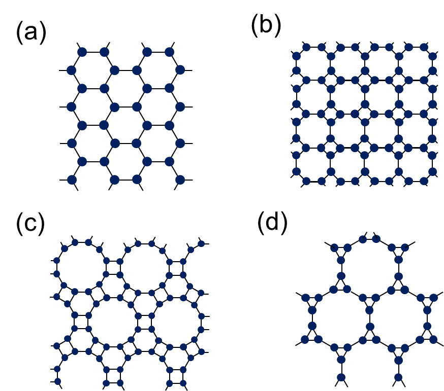
Figure 1: (color online) The four trivalent Archimedean lattices. (a) the honeycomb $(6^{3})$; (b) the square octagon $(4,8^{2})$; (c) the cross $(4,6,12)$; and (d) the star $(3,12^{2})$.

It was shown, by the author and his collaborators WeiAffleckRaussendorf11 and independently by Miayke Miyake11 , that the intrinsic 2D AKLT state on the honeycomb lattice indeed provides a universal resource for MBQC. The notion of the computational backbone for universal quantum computation was introduced by Miyake in Ref. Miyake11 and his argument that such backbone exists in the honeycomb lattice seems intuitive. The key point of his argument is that the backbone consists mainly of the sites that have different POVM outcomes with their neighbors as well as the edges that link these sites Miyake11 . For a pair of neighboring sites, the six outcomes: $xy$, $xz$, $yx$, $yz$, $zx$, $zy$ are desirable whereas the remaining three $xx$, $yy$, $zz$ do not contribute to the backbone. This corresponds approximately to the probability that an edge occupied by the backbone being $p_{\rm occ}=2/3$. Because the bond percolation threshold for the honeycomb lattice is $p_{th}^{\rm(bond)}\approx 0.65<p_{\rm occ}$, the computational backbone spanning across the lattice exists and thus the AKLT state is a universal resource. However, as we shall see below that the argument cannot extend to other trivalent lattices with $p_{th}>2/3$.

So far the 2D AKLT state on the honeycomb lattice is the only state in the AKLT family that has been shown to be a universal resource. It is unclear whether its computational universality is a coincidence or a more general feature in the family of two-dimensional AKLT states. From the viewpoint of magnetic ordering, in three dimensions, AKLT states can be Néel ordered on many lattices such as the cubic lattice, but they can also be disordered on lattices such as diamond and pyrochlore Param . But all 2D AKLT states are found to be disordered. Néel ordered states are believed not to possess sufficient quantum correlation for the MBQC. Is being disordered in 2D or higher sufficient for the AKLT states to be universal for MBQC? In contrast for cluster states, it has been shown that all 2D cluster states (i.e., graph states on all 2D regular lattices; see also Sec. II.1), including those on the square, triangular, honeycomb, and Kagome lattices, are all universal Universal .

Here, we focus ourselves on the family of spin-3/2 AKLT states but on various trivalent Archimedean lattices, which include the honeycomb $(6^{3})$, the square octagon $(4,8^{2})$, the ‘cross’ $(4,6,12)$ and the ‘star’ $(3,12^{2})$ lattices; see Fig. 1. All latter three lattices have bond percolation thresholds higher than $2/3$, in contrast to the honeycomb lattice, which has the threshold approximately $0.65$. Does this mean that AKLT states on these trivalent lattices but the honeycomb are not universal, i.e., cannot be used to implement universal MBQC? Surprisingly, as we shall find below, in addition to the honeycomb lattice, the spin-3/2 AKLT states on the square octagon and the cross lattices are also universal resources, whereas the spin-3/2 AKLT state on the star $(3,12^{2})$ lattice is likely not due to geometric frustration; see Table 1 for a summary. Along the way, we have also provided an efficient method for the Metropolis update, improving on the accessible system sizes that previous works could achieve WeiAffleckRaussendorf11 ; WeiAffleckRaussendorf12 ; DarmawanBrennenBartlett .

The remaining of the paper is organized as follows. In Sec. II we define the AKLT, graph and cluster states. In Sec. III we describe the procedure to convert an AKLT state to a graph state by POVM. If the resulting graph state lies in the supercritical phase, then it can be used for universal quantum computation. In Sec. IV we describe an efficient Metropolis update method and perform numerical simulations for AKLT states on various trivalent Archimedean lattices. Unlike the other lattices (honeycomb, square octagon and cross), the star lattice possesses geometric frustration and the associated AKLT state is argued to fail to provide a universal resource. In Sec. V we make some concluding remarks.

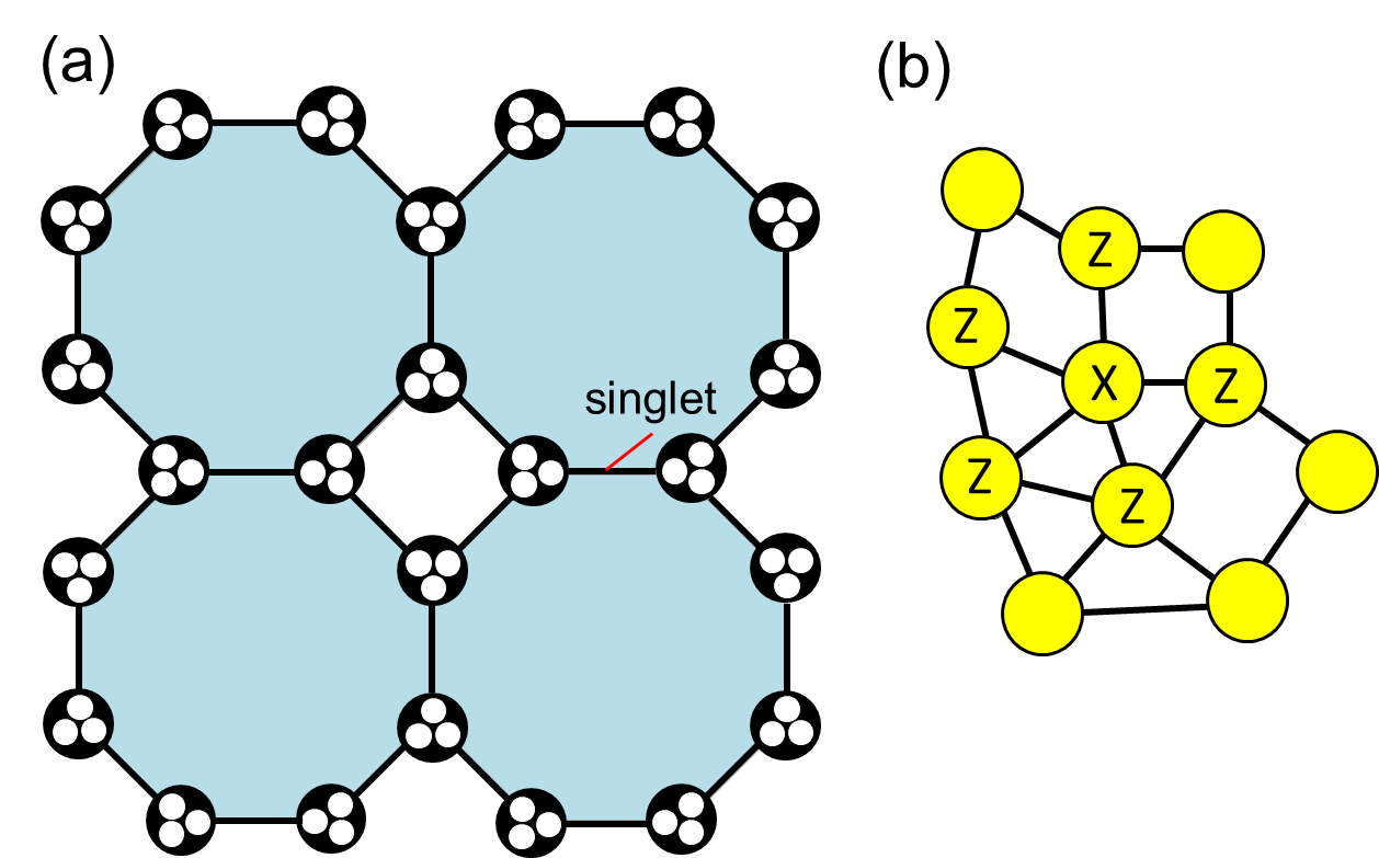
Figure 2: (color online) Illustrations of the AKLT state on a square-octagon lattice and a graph state on a graph. (a) AKLT state. Each site is spin-3/2 and can be regarded as three virtual spin-1/2’s in their symmetric subspace. Two virtual qubits connected by an edge form a spin singlet state. (b) A graph state. One qubit resides at each vertex and one stabilizer generator of the form $X\otimes Z\cdots Z$ is shown (with $X\equiv\sigma_{x}$ at a vertex and $Z\equiv\sigma_{z}$ on neighboring vertices). Cluster states are graph states defined on regular lattices.

II AKLT and cluster states

Let us now define the spin-3/2 AKLT states, the graph and cluster states. The AKLT state AKLT on the trivalent Archimedean lattices ${\cal{L}}$ (see Fig. 1) has one spin-3/2 per site of lattice ${\cal{L}}$. The state space of each spin 3/2 can be viewed as the symmetric subspace of three virtual spin-1/2’s, i.e., qubits. In terms of these virtual qubits, the AKLT state on ${\cal{L}}$ is (see Fig. 2a)

$$|\Phi_{\rm AKLT}\rangle\equiv\bigotimes_{v\in V({\cal{L}})}P_{S,v}\bigotimes_{e\in E({\cal{L}})}|\phi\rangle_{e},$$ (1)

where $V({\cal L})$ and $E({\cal L})$ to denote the set of vertices and edges of ${\cal L}$, respectively. $P_{S,v}$ is the projection onto the symmetric (equivalently, spin 3/2) subspace at site $v$ of ${\cal{L}}$ WeiAffleckRaussendorf11 ; WeiAffleckRaussendorf12 . For an edge $e=(v,w)$, $|\phi\rangle_{e}$ denotes a singlet state, with one virtual spin 1/2 at vertex $v$ and the other at $w$. On the other hand, a graph state $|G\rangle$ is a stabilizer state Hein with one qubit per vertex of the graph $G$ (see Fig. 2b) and is the unique eigenstate of a set of commuting operators Cluster , usually called the stabilizer generators Stabilizer ,

$$\sigma_{x}^{[v]}\bigotimes_{u\in{\rm nb}(v)}\sigma_{z}^{[u]}\,\,|{G}\rangle=|{G}\rangle,\ \forall v\in V({G}),$$ (2)

where ${\rm nb}(v)$ denotes the neighbors of vertex $v$, and $\sigma_{x}$, $\sigma_{y}$ and $\sigma_{z}$ are the Pauli matrices. The original cluster state was defined as the graph state on the square lattice, but recent trend is to refer to any graph state with the underlying graph being a regular lattice as a cluster state. We shall adopt this broader definition of a cluster state.

II.1 Remarks on universality of 2D cluster states and other graph states

It was shown by Van den Nest et al. Universal that the graph states on the triangular, honeycomb, and Kagome lattices can all be converted to graph states on the square lattice via local measurement, hence proving that these cluster states also provide the same quantum computational power as the square-lattice cluster state. Their approach can be applied to show that the cluster states on the square-octagon, cross and star lattices are also universal, the proof of which is given in Appendix A. Browne et al. Browne considered faulty cluster states on the square lattice, i.e., graph states whose graphs are obtained from square lattice by site deletion and are thus irregular. Such irregular graph states (from site deletion) are universal if the site occupation probability is below the site percolation threshold of the square lattice. Their treatment was subsequently generalized to general 2D random graphs, and naturally the universality of the corresponding graph states arises if the graphs are in the supercritical phase of percolation WeiAffleckRaussendorf12 . On the other hand, even though AKLT states can be defined on any graph, their fate of universality is much less understood. As detailed below, our proof of universality for the trivalent AKLT states relies on reduction of them to graph/cluster states via a particular local generalized measurement (3). If the reduction from AKLT states to universal graph states can be shown, then the universality of the AKLT states is thus established. However, to prove that a particular AKLT state is not universal, one may need to show that for all possible local measurement, such a reduction to universal graph states is not possible. Other possible approaches for proving non-universality include the scaling of entanglement Universal and efficient classical simulation VandenNestDurVidalBriegel07 . These latter methods seems unlikely useful for proving non-universality for 2D AKLT states, as they possess entanglement that satisfies an area law and the tensor network description for all trivalent AKLT states gives essentially the same local tensors.

(a)	(b)

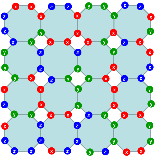
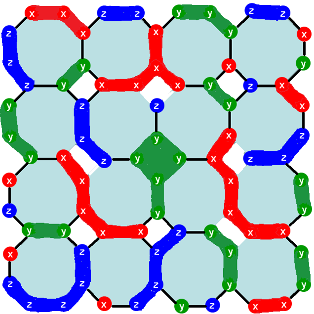
Figure 3: (color online) Illustration of POVM outcomes and construction of the graph for the resulting graph state on a square-octagon lattice. (a) POVM outcomes: x (red), y (green) and z (blue). (b) The graph after formation of domains and edge modulo-2 operation.

III From AKLT to graph states

The AKLT state on the honeycomb lattice was shown, via two different approaches, in Ref. WeiAffleckRaussendorf11 and Ref. Miyake11 , respectively, to be a universal resource. In the former WeiAffleckRaussendorf11 a generalized measurement or positive-operator-value-measure measurement (POVM), see below, on all spins gives rises to a random planar graph state $|G({\cal{A}})\rangle$, whose graph $G({\cal{A}})$ possesses a macroscopic number of vertices and connections and from which a 2D cluster state can be carved out by local measurement. Here, ${\cal A}$ denotes the set measurement outcomes on all sites; see Figs. 3 and 4 for example. In the latter Miyake11 the same POVM was used but universal gates were constructed and a computational backbone on the honeycomb lattice was argued to exist. Its existence relies on the bond percolation threshold of the honeycomb lattice being smaller than $2/3$, as explained earlier. For all the lattices that we shall examine, their bond percolation thresholds are all higher than $2/3$ (approximately, $0.6768$ for the square-octagon, $0.6737$ for the cross, and $0.7404$ for the star, respectively). This suggests that either the AKLT states on these lattices may not be universal for MBQC or the argument used in Ref. Miyake11 simply cannot be extended to these cases. Therefore, to determine whether they can be universal, we shall follow the approach employed in Ref. WeiAffleckRaussendorf11 , where the argument that, after the POVM, the AKLT state is mapped to a random planar graph state $|G({\cal{A}})\rangle$ applies more generally and, specifically, to other trivalent AKLT states. The MBQC on cluster and graph states rely on the ability to simulate multiple-qubit evolution along quantum wires and interaction between qubits on neighboring wires. The computational universality of typical graph states $|G({\cal{A}})\rangle$ hence is dependent on the connectivity of $G({\cal{A}})$, and thus the problem whether these AKLT states are universal resource can be resolved by examining the properties of the typical graphs resulting from the POVM.

Let us elaborate on one of the key steps in the construction, i.e., the POVM. The approach we shall use is to convert locally four-level spin-3/2 particles to two-level qubits, and this requires projection or, more generally, a local generalized measurement NielsenChuang00 (or POVM), on every site $v$ on ${\cal{L}}$. The POVM consists of three rank-two elements

$$\!\!\!\!{F}_{v,z}\!\!\!\!\!\!\!\! =\sqrt{\frac{2}{3}}(|000\rangle\langle 000|+|111\rangle\langle 111|)$$

$$= \sqrt{\frac{2}{3}}\Big{(}|S_{z}=\frac{3}{2}\rangle\langle S_{z}=\frac{3}{2}|+|S_{z}=-\frac{3}{2}\rangle\langle S_{z}=-\frac{3}{2}|\Big{)}$$

$$\!\!\!\!{F}_{v,x}\!\!\!\!\!\!\!\! =\sqrt{\frac{2}{3}}(|+++\rangle\langle+++|+|---\rangle\langle---|)$$

$$= \sqrt{\frac{2}{3}}\Big{(}|S_{x}=\frac{3}{2}\rangle\langle S_{x}=\frac{3}{2}|+|S_{x}=-\frac{3}{2}\rangle\langle S_{x}=-\frac{3}{2}|\Big{)}$$

$$\!\!\!\!{F}_{v,y}\!\!\!\!\!\!\!\! =\sqrt{\frac{2}{3}}(|i,i,i\rangle\langle i,i,i|+|-\!i,-\!i,-\!i\rangle\langle-\!i,-\!i,-\!i|)$$

$$= \sqrt{\frac{2}{3}}\Big{(}|S_{y}=\frac{3}{2}\rangle\langle S_{y}=\frac{3}{2}|+|S_{y}=-\frac{3}{2}\rangle\langle S_{y}=-\frac{3}{2}|\Big{)},$$

where $|0/1\rangle$, $|\pm\rangle\equiv(|0\rangle\pm|1\rangle)/\sqrt{2}$ and $|\pm i\rangle\equiv(|0\rangle\pm i|1\rangle)/\sqrt{2}$ are eigenstates of the Pauli operators $\sigma_{z}$, $\sigma_{x}$ and $\sigma_{y}$, respectively. As indicated in the second line of each of the above three equations, physically, $F_{v,a}$ is proportional to a projector onto the two-dimensional subspace spanned by the $S_{a}=\pm 3/2$ states. Its action on the rotationally invariant AKLT state gives a locally preferred quantization axis $a$. The above POVM elements obey the relation $\sum_{\nu\in\{x,y,z\}}F^{\dagger}_{v,\nu}F_{v,\nu}=P_{S,v}$ in terms of three qubits, i.e., the sum projects onto the symmetric subspace, as required, or equivalently equals identity in terms of spin-3/2 states. Such POVM can, in principle, be implemented by coupling the local spin (whose initial state denoted by $|\psi\rangle_{v}$) to a meter (whose initial state denoted by $|0\rangle_{m}$) so that the spin and meter involve unitarily:

$$U:\ |\psi\rangle_{v}\otimes|0\rangle_{m}\rightarrow\sum_{a=x,y,z}F_{v,a}|\psi\rangle_{v}\otimes|a\rangle_{m},$$ (4)

where $|x\rangle_{m}$, $|y\rangle_{m}$, and $|z\rangle_{m}$ are three orthogonal meter states. Upon ‘reading’ the meter state to be $|a\rangle_{m}$, the spin state ‘collapses’ to $F_{v,a}|\psi\rangle_{v}$. We note that the unitary transformation $U$ in Eq. (4) can always be found and is not unique NielsenChuang00 .

(a)	(b)

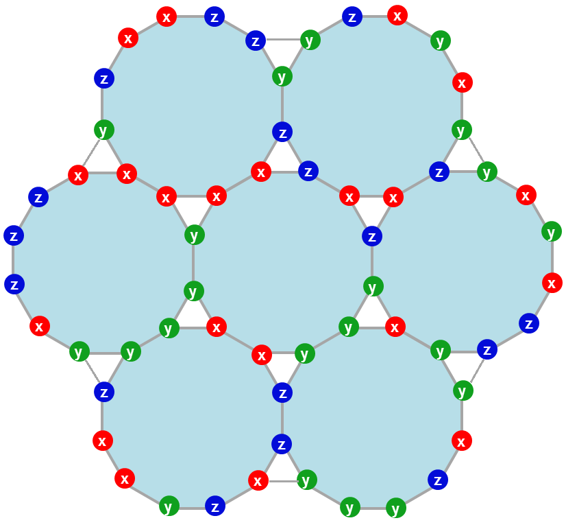
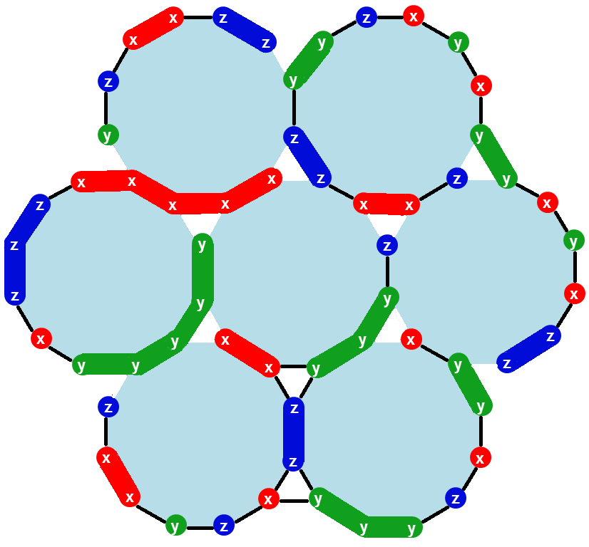
Figure 4: (color online) Illustration of POVM outcomes and construction of the graph for the resulting graph state on a star lattice. (a) POVM outcomes: x (red), y (green) and z (blue). (b) The graph after formation of domains and edge modulo-2 operation. One can also see the effect of the geometric frustration, which causes two edges in some triangles to be removed.

In contrast to usual projection operators where there are some probability of getting undesired outcomes (i.e., lying in the orthogonal subspaces to the desired outcomes), here any outcome of the POVM is a successful mapping from four levels to two levels. The outcome $a_{v}$ of the POVM at any site $v$ is random, which can be $x$, $y$ or $z$, but it is correlated with the outcomes at other sites due to quantum correlations in the AKLT state AKLT . As shown in Refs. WeiAffleckRaussendorf11 ; WeiAffleckRaussendorf12 , the resulting quantum state, dependent on the random POVM outcomes ${\cal{A}}=\{a_{v},v\in V({\cal{L}})\}$,

$$|\Psi({\cal{A}})\rangle=\bigotimes_{v\in V({\cal{L}})}\!\!F_{v,a_{v}}\,|\Phi_{\rm AKLT}\rangle$$ (5)

is equivalent to an encoded graph state ${|G({\cal{A}})\rangle}$.

One important consequence of the POVM is that a logical qubit, which sits on a domain (a vertex of $G({\cal{A}})$), can be composed of multiple spins (i.e. those spins whose sites are connected and whose POVM outcomes are the same). Such encoding originates from the antiferromagnetic property inherent in AKLT states: neighboring spin-3/2 particles must not have the same $S_{a}=3/2$ (or -3/2) configuration AKLT . Hence, after the projection onto $S_{a}=\pm 3/2$ subspace by the POVM, the configurations for all sites inside a domain can only be $|3/2,-3/2,3/2,-3/2,\dots\rangle$ or $|-3/2,3/2,-3/2,3/2,\dots\rangle$, and these form the basis or the encoding of a single qubit. This corresponds to that a domain is formed by contracting all edges that connect sites with the same POVM outcome. Equivalently, those edges that are contracted become internal edges of a domain. We note that even though a logical qubit is encoded by several physical spins, the quantum information it carries can be concentrated to any one of the spins, by measuring other spins in the basis $\{|3/2\rangle\pm|-3/2\rangle\}$, still requiring only local measurements.

The graph for the corresponding graph state is formed by domains as vertices. What about the (external) edges? When multiple sites are merged into a domain, two domains can share multiple edges. It turns out that in accordance with the fact that Pauli $\sigma_{z}$ squares to identity (i.e. $\sigma_{z}^{2}=I$), the edges between two domains should be regarded in a modulo two fashion (i.e. edge modulo-2 operation): one should delete all edges of even multiplicity and convert all edges of odd multiplicity into one single edge. See Figs. 3 and 4 for illustration of domain formation and edge modulo-2 operation.

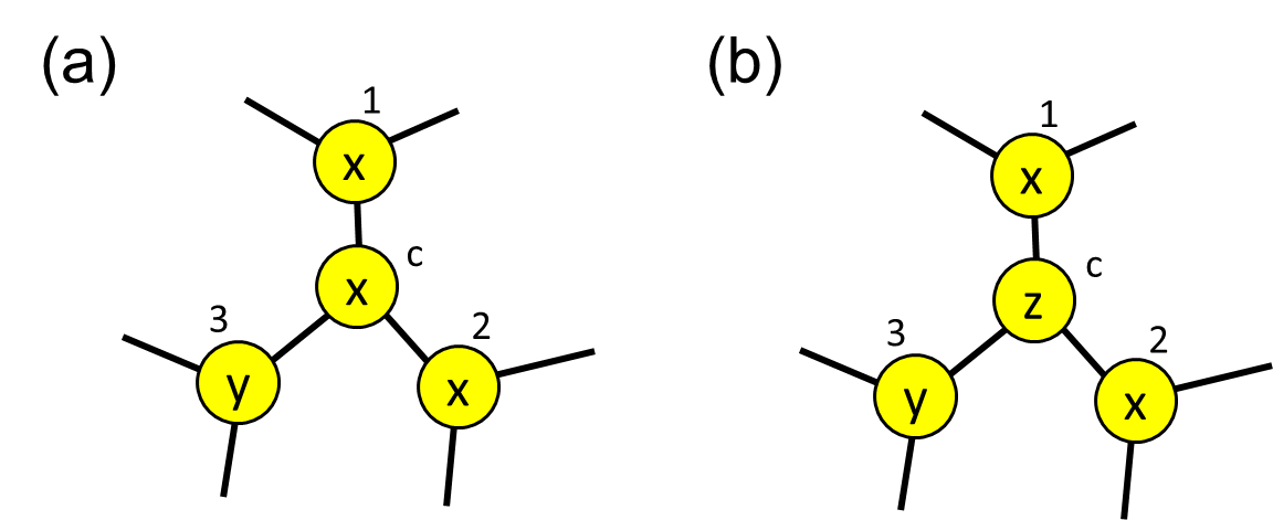
Figure 5: (color online) Illustrations of the counting of $e_{I}$ and $v_{c}$ (see text). The POVM types are shown in the circles: (a) before the type at $c$ was flipped; (b) after it was flipped. In (a), $e_{I}=2$, arising from edges $(c,1)$ and $(c,2)$. In (b) the type on $c$ is flipped from $x$ to $z$ and it is easy to see that $e_{I}=0$. In (a), there are two distinct domains ($v_{c}=2$) that vertices $c$, $1$, $2$ and $3$ belong to. In (b) $v_{c}=3$ if vertices $1$ and $2$ belong to the same domain; otherwise $v_{c}=3$.

IV Efficient Metropolis update and numerical simulations

We used a Monte Carlo method to sample typical random graphs resulting from the POVM and compute their properties. All Archimedean lattices can be embedded on rectilinear grids, enabling simple labeling of sites and their connections SudingZiff . The simulations utilize a generalized Hoshen-Kopelman algorithm HoshenKopelman to identify domains WeiAffleckRaussendorf11 ; WeiAffleckRaussendorf12 . Due to the entanglement in the AKLT states, the local POVM outcomes are correlated which is fully taken into account in our simulations. In particular, to sample typical POVM outcomes ${\cal A}$ correctly, we use a Metropolis method to update configurations. For each site we attempt to flip the type (either $x$, $y$ or $z$) to one of the other two equally and accept the flip with a probability

$$p_{\rm acc}=\min\big{\{}1,2^{|V^{\prime}|-|{\cal E}^{\prime}|-|V|+|{\cal E}|}\big{\}},$$ (6)

where $|V|$ and $|{\cal E}|$ denote the number of domains and inter-domain or external edges (without the edge modulo-2 operation), respectively, before the flip, and similarly $|V^{\prime}|$ and $|{\cal E}^{\prime}|$ for the flipped configuration WeiAffleckRaussendorf12 . We note that in terms of the set of internal edges, denoted by ${\cal E}_{I}$, we have that $|{\cal E}|+|{\cal E}_{I}|={\rm const.}$ Then the above equation can be replaced by $p_{\rm acc}=\min\big{\{}1,2^{|V^{\prime}|+|{\cal E}_{I}^{\prime}|-|V|-|{\cal E}_{I}|}\big{\}}$.

The probability in Eq. (6) involves global quantities $|{\cal E}|$ and $|V|$. But do we have to compute $|{\cal E}|$, $|V|$, $|{\cal E}^{\prime}|$ and $|V^{\prime}|$ every time when we attempt to flip the type of a site, as was done in Refs. WeiAffleckRaussendorf11 ; WeiAffleckRaussendorf11 ; DarmawanBrennenBartlett ? The probability ratio can actually be replaced by a quasi-local quantity. Denote by $e_{I}$ the number of internal edges impinging on a vertex $c$ and $v_{c}$ the total number of distinct domains that the site $c$ and its neighbors belong to. The quantity $e_{I}$ can be straightforwardly checked locally by comparing the POVM type on $c$ and those on its neighbors; see Fig. 5. To count the distinct domains, we first apply a Wolff algorithm Wolff to grow domains on $c$ and the remaining sites of its neighbors (that are not yet included in a domain) and then check the total number of distinct domains. This can be done quasi-locally and in the worst case scenario the largest domain has a size logarithmic in the system size. Similarly, we can compute the $e_{I}^{\prime}$ and $v_{c}^{\prime}$ when the POVM type on $c$ is flipped. Thus, we arrive at

$$p_{\rm acc}=\min\big{\{}1,2^{v_{c}^{\prime}+e_{I}^{\prime}-v_{c}-e_{I}}\big{\}}.$$ (7)

With such a local update, the system size can reach to $N=L^{2}$ with $L\sim 1000$ without any difficulty. (Results of $L\sim 500$ and $\sim 1000$ are illustrated, e.g., in Figs. 6 and 8, and are consistent with those from smaller sizes.)

In the square-octagon and cross lattices, all the $3^{N}$ possible POVM outcome configurations can occur. But in the case of the star lattice, due to geometric frustration, the three sites in a triangle cannot share the same POVM outcome. This is taken care of by excluding the initial random assignment to be such configurations and by forbidding transition to such configurations during the simulations.

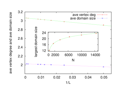
Figure 6: (color online) Average domain size, average degree of a vertex, and the largest domain size (inset) in the typical graphs vs. $L=20,40,60,80,100,120,500,1000$, with $N=L^{2}$ being the total number of sites for the square-octagon lattice. Inset: The largest domain size scales with $N$ logarithmically.

(a)

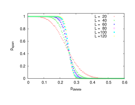
(b)

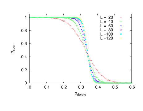
Figure 7: (color online) Percolation study of the random graphs of domains resulting from the original square-octagon lattice: probability of a spanning cluster $p_{\rm span}$ vs. that to delete an edge $p_{\rm delete}$ with $N=L^{2}$. (a) Site percolation and (b) bond percolation.

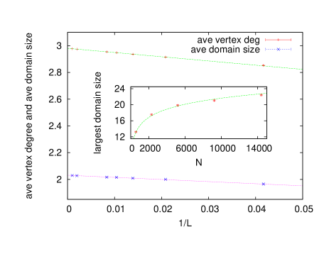
Figure 8: (color online) Average domain size, average degree of a vertex, and the largest domain size (inset) in the typical graphs vs. $L=24,48,72,96,120,504,1008$, with $N=L^{2}$ being the total number of sites for the cross lattice. Inset: The largest domain size scales with $N$ logarithmically.

(a)

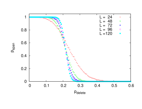
(b)

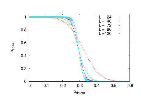
Figure 9: (color online) Percolation study of the random graphs of domains resulting from the original cross lattice: probability of a spanning cluster $p_{\rm span}$ vs. that to delete an edge $p_{\rm delete}$ with $N=L^{2}$. (a) Site percolation and (b) bond percolation.

IV.1 Square-octagon and cross lattices

For the square-octagon and cross lattices, we have tested that all the typical graphs of the post-POVM graph states are percolated and deep in the supercritical phase, by randomly deleting a fraction of vertices or edges from $G({\cal{A}})$. For the square-octagon lattice, the average domain size is $2.025(2)$ the average degree $\bar{d}\approx 3.065(1)$ (see Fig. 6). There remain macroscopic number of vertices and edges: the number of vertices $|\bar{V}|\approx 0.488(1)N$, the number of edges $|\bar{E}|\approx 0.748(1)N$. The typical graphs after the POVM reside deep in the supercritical phase of percolation, as evidenced by the fact that the threshold for site deletion is $p^{\rm[site]*}_{\rm delete}\approx 0.26(1)$ and the threshold for edge deletion is $p^{\rm[bond]*}_{\rm delete}\approx 0.35(1)$; see Fig. 7. The corresponding site and bond percolation thresholds ($p_{\rm th}=1-p_{\rm delete}$) are $0.74(1)$ and $0.65(1)$, respectively.

For the cross lattice, the average domain size is $2.029(2)$, the average degree $\bar{d}\approx 2.980(1)$ (see Fig. 8). Similar to the square-octagon case, there also remain macroscopic number of vertices and edges: the number of vertices $|\bar{V}|\approx 0.485(1)N$, the number of edges $|\bar{E}|\approx 0.723(1)N$. Furthermore, the typical graphs after the POVM reside deep in the supercritical phase of percolation, as evidenced by the fact that the threshold for site deletion is $p^{\rm[site]*}_{\rm delete}\approx 0.21(1)$ and the threshold for edge deletion is $p^{\rm[bond]*}_{\rm delete}\approx 0.29(1)$; see Fig. 9. The corresponding site and bond percolation thresholds ($p_{\rm th}=1-p_{\rm delete}$) are $0.79(1)$ and $0.71(1)$, respectively. Table 1 contains a summary of all these properties, including those from the honeycomb AKLT state.

Let us examine the consequence of the above results in the context of quantum computational universality. Whether or not typical graph states $|G({\cal{A}})\rangle$ are universal resources hinges solely on connectivity properties of $G({\cal{A}})$ (provided the graph is macroscopic), and is thus a percolation problem Perc . Two simple criteria can be used to determine whether the AKLT states on the trivalent lattices ${\cal L}$ are universal WeiAffleckRaussendorf11 ; WeiAffleckRaussendorf12 :

1. The distribution of the number of sites in a domain (i.e. domain size) is microscopic, i.e., the largest domain size can at most scale logarithmically with the total number of sites $|V({\cal{L}})|$ in the large ${\cal{L}}$ limit.

2. The probability of the existence of a path through $G({\cal{A}})$ from the left to the right (or top to bottom) approaches unity in the limit of large ${\cal{L}}$.

Condition C1 ensures that the graph $G({\cal{A}})$ remains macroscopic, i.e., possesses macroscopic number of vertices and edges, if the original ${\cal{L}}$ was. Condition C2 ensures that the system is in the supercritical phase with a macroscopic spanning cluster of domains, and hence there exist sufficient number of paths that can be used to simulate evolution of qubits (such as single qubit gates) and their interactions (such as the CNOT gate). For a large initial lattice ${\cal{L}}$ the random graph state $|G({\cal{A}})\rangle$ resulting from the POVM can thus be efficiently reduced to a large two-dimensional cluster state WeiAffleckRaussendorf12 .

It is evident that the results of our numerical simulations demonstrate that both conditions C1 and C2 are satisfied in the cases of the square-octagon and cross lattices. This shows that they are both universal resources for MBQC.

(a)

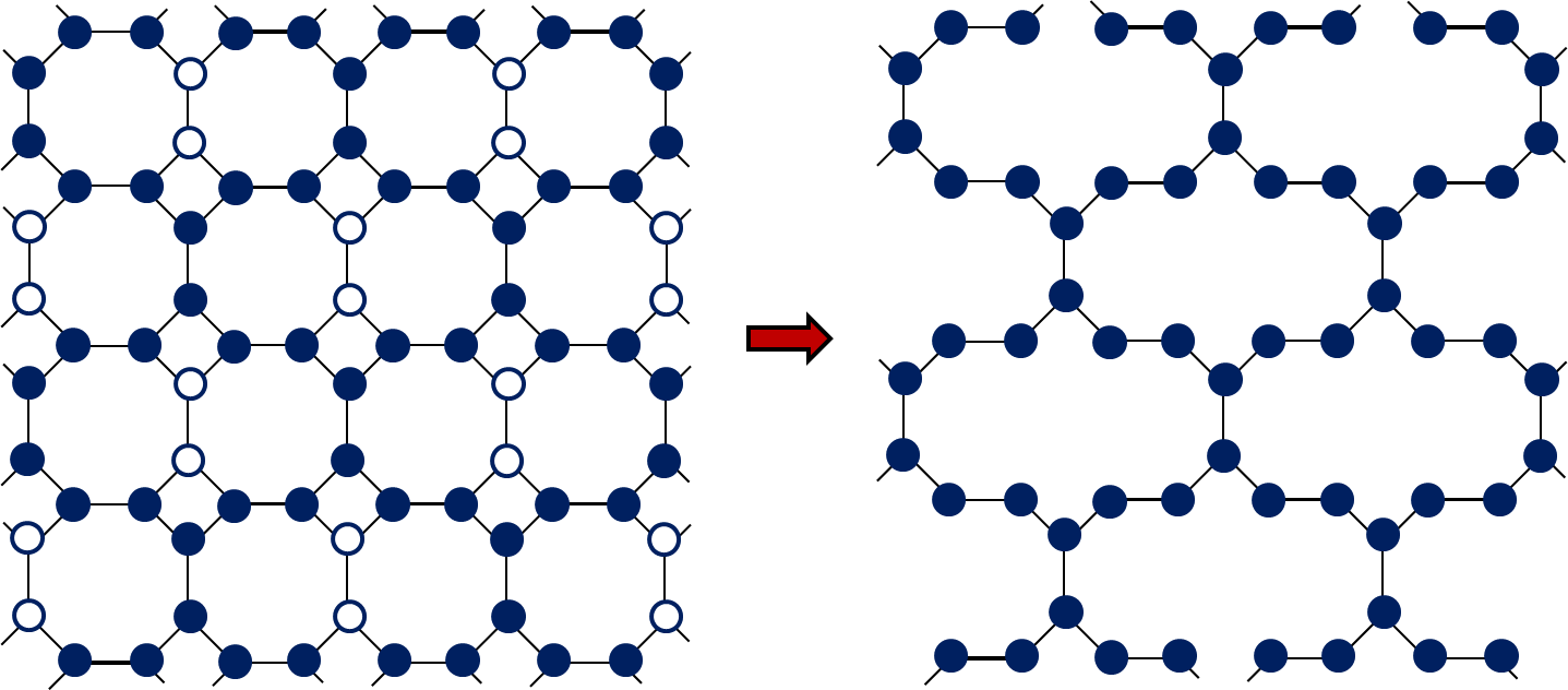
(b)

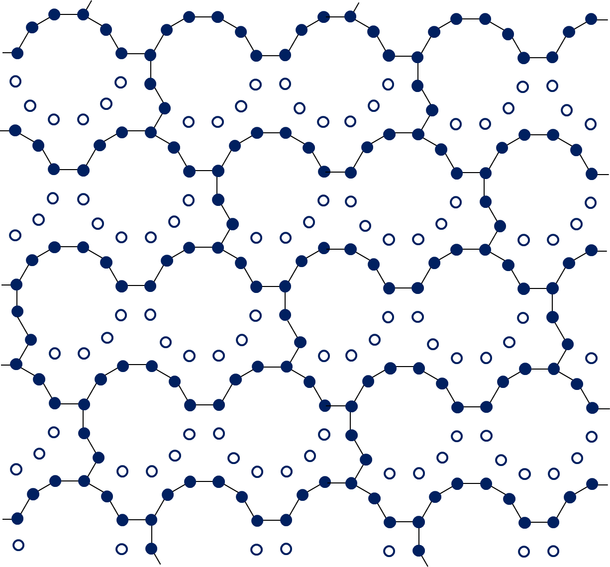
Figure 10: (color online) Illustration of the key local measurement in converting the cluster states on (a) the square-octagon and (b) the cross lattices to a cluster state on the honeycomb lattice. The hollow circles indicate the locations where Pauli Z measurement is performed. The picture on the r.h.s. in (a) shows the resulting graph after removing the Z measured sites, which is topologically equivalent to a honeycomb lattice, except with additional sites of vertex degree 2. In (b) the resultant graph is shown by removing the edges due to Z measurements on the sites indicated by hollow circles. In both cases, Pauli X measurements can be applied to those sites of vertex degree 2 to further reduce to the honeycomb lattice.

IV.2 The star lattice

For the star lattice, however, none of the typical POVM configurations that we generated (for $L\geq 48$) yield percolated graphs, i.e., they reside in the subcritical phase, even without any deletion of vertices or edges. This shows that there does not exist a computational backbone (formed by domains) that extends to a two-dimensional grid and thus there are not sufficient paths to simulate evolution of qubits and their interaction. Hence, the resultant graph states cannot be used to perform universal quantum computation. We should stress that for a finite system the POVM can, albeit with a probability exponentially small with the system size, yield graph states (e.g. a cluster state on the original star lattice) whose graphes are indeed percolated, consistent with our simulations. However, we are concerned with the ability to generate universal resource states in the large system limit. In this limit, the probability that one obtains graph states that are universal approaches zero, consistent with our numerical simulations as we increases the system size.

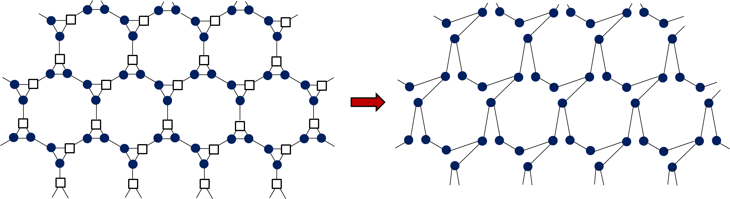
Figure 11: (color online) Illustration of the key local measurement in converting the cluster state on the star lattice to a cluster state on the honeycomb lattice. The hollow squares indicate the locations where Pauli Y measurement is performed. The action of Pauli Y measurement is to perform local complementation followed by removal of the vertex measured. The resultant graph is shown on the r.h.s., which is topologically equivalent to a honeycomb lattice. Pauli X measurements can be applied to those sites of vertex degree 2 to further reduce to the honeycomb lattice.

This lack of universality for the resultant typical graph states is due to the antiferromagnetic property of the original AKLT state and the geometric frustration in the star lattice. An intuitive understanding is as follows. Consider a triangle and because of geometric frustration, the POVM outcome with $(x,x,x)$, $(y,y,y)$ and $(z,z,z)$ cannot occur. There are 6 outcomes with all three labels be different (case 1) and 18 outcomes with only two labels being the same and the third being distinct (case 2). In the former case the three edges remain, whereas in the latter case two of the three edges are removed (and the remaining one becomes an internal edge). This gives rise to an average probability of $p_{\rm delete}^{\rm[bond]}=1/4*0+3/4*2/3=1/2$ to remove an edge in an triangle. The edges that connect neighboring triangles either become internal edges or remain external edges (see Fig. 4). Hence for the purpose of percolation, we can consider contracting these edges and thus the star lattice becomes a Kagome lattice, which has a bond percolation threshold $p_{\rm th}^{\rm[bond]}\approx 0.5244$. Thus deleting an edge with probability $1/2$ will make the graph become un-percolated. We note that consideration of correlated removal of edges should be taken into account. Our numerical simulations do take into account all correlations in the configuration (and hence correlations in removing edges) and confirm that the graphs resulting from the POVM are in the subcritical phase. This implies that the AKLT state on the star lattice under the POVM cannot produce a graph state that is universal for MBQC, which fails to satisfies Condition C2 (percolation). In contrast, the Néel phase in the deformed AKLT model on the honeycomb lattice NiggemannKlumperZittarz was argued not universal due to the breaking of Condition C1 (non-macroscopic domains) DarmawanBrennenBartlett . We should emphasize that we have not ruled out the possibility that other POVM’s might enable the star-lattice AKLT state for universal MBQC, even though we believe that it is unlikely. On another note, frustrated lattices such as the star and Kagome lattices are of particular interest in condensed matter physics, as they can host exotic phases of matter, such as the spin liquids YaoKivelson ; YangParamekantiKim ; YanHuseWhite . Here, we have witnessed evidence that such frustration may prevent a certain type of universal resource states to exist.

V Concluding remarks

Given that the spin-3/2 AKLT state on the honeycomb lattice has been shown to be a universal resource for MBQC, a natural question arises whether other AKLT states can also be universal. We have thus investigated MBQC with the spin-3/2 AKLT states on all four trivalent Archimedean lattices and found that they are also universal on two other lattices: the square-octagon $(4,8^{2})$ and the cross $(4,6,12)$. Furthermore, the same POVM performed on the AKLT state on the star lattice $(3,12^{2})$ yields typical graph states whose graphs are in subcritical phase (in the sense of percolation), and this suggests the AKLT state on the star lattice may not be universal for MBQC. However, it might be possible that other POVM’s could turn this AKLT state into a universal resource, which, remains an open question.

Acknowledgment. The author thanks Ian Affleck and Robert Raussendorf for useful discussions. This work was supported by the National Science Foundation under Grants No. PHY 1314748 and No. PHY 1333903.

Appendix A Cluster states on trivalent Archimedean lattices

The cluster state on one of the four trivalent Archimedean lattices, namely, the honeycomb lattice, was shown by Van den Nest et al. to be universal for MBQC Universal . Their approach is to use local Pauli measurements and their effects on the original graph is to transform it with certain rules Universal ; Hein2 . For example, a Pauli Z measurement on a qubit corresponds to deleting edges incident to the vertex that the qubit resides on, hence disentangling the qubit (whose vertex is removed as well). A Pauli Y measurement on a qubit corresponds to first implementing the local complementation on the neighboring vertices, followed by removing the measured vertex and edges incident on it. Using these rules, we can prove that the all the cluster states on the square-octagon, cross and star lattices can be converted to a cluster state on the honeycomb lattice, which is universal. The key step for all three cases are illustrated in Figs. 10& 11.

References

- (1) M. Nielsen and I. Chuang, Quantum Computation and Quantum Information (Cambridge Univ. Press, 2000).
- (2) R. Raussendorf and H. J. Briegel, Phys. Rev. Lett. 86, 5188 (2001).
- (3) H. J. Briegel, D. E. Browne, W. Dür, R. Raussendorf, and M. Van den Nest, Nature Phys. 5, 19 (2009).
- (4) R. Raussendorf and T.-C. Wei, Annu. Rev. Condens. Matter Phys. 3, pp.239-261 (2012).
- (5) M. Van den Nest, W. Dür, G. Vidal, and H. J. Briegel, Phys. Rev. A 75, 012337 (2007).
- (6) M. Van den Nest, W. Dür, A. Miyake, and H. J. Briegel, New J. Phys. 9, 204 (2007).
- (7) D. Gross, S.T. Flammia, and J. Eisert, Phys. Rev. Lett. 102, 190501 (2009); M.J. Bremner, C. Mora, and A. Winter, ibid 102, 190502 (2009).
- (8) H. J. Briegel and R. Raussendorf, Phys. Rev. Lett. 86, 910 (2001).
- (9) M. A. Nielsen, Rep. Math. Phys. 57, 147 (2006).
- (10) D. Gross and J. Eisert, Phys. Rev. Lett. 98, 220503 (2007).
- (11) F. Verstraete and J. I. Cirac, Phys. Rev. A 70, 060302(R) (2004).
- (12) X. Chen, B. Zeng, Z.-C. Gu, B. Yoshida, and I. L. Chuang, Phys. Rev. Lett. 102, 220501 (2009).
- (13) I. Affleck, T. Kennedy, E. H. Lieb, and H. Tasaki, Phys. Rev. Lett. 59, 799 (1987).
- (14) I. Affleck, T. Kennedy, E. H. Lieb, and H. Tasaki, Comm. Math. Phys. 115, 477 (1988).
- (15) G. K. Brennen and A. Miyake, Phys. Rev. Lett. 101, 010502 (2008).
- (16) F. D. M. Haldane, Phys. Lett. A 93, 464-468 (1983).
- (17) F. D. M. Haldane, Phys. Rev. Lett. 50, 1153-1156 (1983).
- (18) T. Kennedy, E. H. Lieb, and H. Tasaki, J. of Stat. Phys. 53, 383 (1988).
- (19) R. Kaltenbaek , J. Lavoie, B. Zeng, S. D. Bartlett, and K. J. Resch, Nature Phys. 6, 850 (2010).
- (20) S. D. Bartlett, G. K. Brennen, A. Miyake, and J. M. Renes, Phys. Rev. Lett. 105, 110502 (2010).
- (21) A. Miyake, Phys. Rev. Lett. 105, 040501 (2010).
- (22) D. V. Else, I. Schwarz, S. D. Bartlett, and A. C. Doherty, Phys. Rev. Lett. 108, 240505 (2012).
- (23) T.-C. Wei, I. Affleck, and R. Raussendorf, Phys. Rev. Lett. 106, 070501 (2011).
- (24) J.-M. Cai, A. Miyake, W. Dür, and H. J. Briegel, Phys. Rev. A 82, 052309 (2010).
- (25) T.-C. Wei, R. Raussendorf, and L. C. Kwek, Phys. Rev. A 84, 042333 (2011).
- (26) A. Miyake, Ann. Phys. (Leipzig) 326, 1656 (2011).
- (27) S. A. Parameswaran, S. L. Sondhi, and D. P. Arovas, Phys. Rev. B 79, 024408 (2009).
- (28) M. Van den Nest, A. Miyake, W. Dür, and H. J. Briegel, Phys. Rev. Lett. 97, 150504 (2006).
- (29) T.-C. Wei, I. Affleck, and R. Raussendorf, Phys. Rev. A 86, 032328 (2012).
- (30) A. S. Darmawan, G. K. Brennen, and S. D. Bartlett, New J. Physics, 14, 013023 (2012).
- (31) M. Hein, J. Eisert, and H.-J. Briegel, Phys. Rev. A 69, 062311 (2004).
- (32) D. Gottesman, Stabilizer Codes and Quantum Error Correction, Ph.D. Thesis, Caltech (1997).
- (33) D. E. Browne, M. B. Elliott, S. T. Flammia, S. T. Merkel, A. Miyake, A. J. Short, New J. Physics 10, 023010 (2008).
- (34) P. N. Suding and R. M. Ziff, Phys. Rev. E 60, 275 (1999).
- (35) J. Hoshen and R. Kopelman, Phys. Rev. B 14, 3438 (1976).
- (36) U. Wolff, Phys. Rev. Lett. 62, 361 (1989).
- (37) R. Durrett, Random Graph Dynamics, Cambridge University Press (2007).
- (38) H. Niggemann, A. Klümper, and J. Zittartz, Z. Phys. B 104, 103 (1997).
- (39) H. Yao and S. A. Kivelson, Phys. Rev. Lett. 99, 247203 (2007).
- (40) B.-J. Yang, A. Paramekanti, and Y. B. Kim, Phys. Rev. B 81, 134418 (2010).
- (41) S. Yan, D. A. Huse, and S. R. White, Science 332, 1173 (2011).
- (42) M. Hein, W. Dür, J. Eisert, R. Raussendorf, M. Van den Nest, and H.-J. Briegel, eprint quant-ph/0602096.