Optical correlation techniques
for the investigation of colloidal systems

Abstract

This review aims to provide a simple introduction to the application of optical correlation methods in colloidal science. In particular, I plan to show that full appraisal of the intimate relation between light scattering and microscopy allows designing novel powerful investigation techniques that combine their powers. An extended version of this paper will appear in Colloidal Foundations of Nanoscience, edited by D. Berti and G. Palazzo, Elsevier (ISBN 978-0-444-59541-6). I am very grateful to the publisher for having granted me the permission to post this preprint on arXiv.

Scattering or microscopy experiments necessarily involve statistical fluctuations, which already stem from the optical source used to probe the investigated system, are modified by the interaction of the probing field with the sample, and are further influenced by the detection process. All these effects concur in turning optical fields into random signals, which are physically described in terms of correlations. In optics, fluctuations and correlations are nicely embodied in the concept of coherence. As the Roman god of beginnings and transitions, Janus, coherence is however two-faced: because the field fluctuates both in time and space, one should indeed distinguish between temporal and spatial coherence. Setting apart these two aspects is not always possible, since they can be intrinsically intermixed, but when this is feasible, it is far more than a useful practical approach. As a matter of fact, it involves an important conceptual distinction: whereas temporal coherence is a physical concept, related to the spectrum of the optical signal generated by the interaction of the incoming field with the sample, which is therefore the actual “source” of the detected radiation, spatial coherence has mostly to do with the source extension, so it is usually (but not always) a geometrical problem. Curiously, in spite of this, spatial coherence is far more important, for the physical problems we shall investigate, than temporal coherence. Nevertheless, it is useful to start by recalling some basic concepts of the latter. We shall first refer to the temporal coherence properties of optical fields, or “first order” optical coherence, to distinguish it from correlations of the intensity, discussed later.

I Basic concepts in statistical optics

I.1 Temporal coherence

Temporal fluctuations can be equivalently discussed in the frequency domain, where it is basically related to non-monochromaticity. For a generically time–varying real field $u^{R}(t)$ with Fourier transform $\mathscr{F}[u^{R}]=\tilde{u}^{R}(\omega)$, it is useful to introduce the associated analytical signalGoodman (1985)

$$u(t)=\frac{1}{\pi}\int_{0}^{\infty}\mathrm{d}\omega\,\tilde{u}^{R}(\omega)\mathrm{e}^{-{\rm i}\omega t}=2\int_{0}^{\infty}\mathrm{d}\nu\,\tilde{u}^{R}(\nu)\mathrm{e}^{-{\rm i}2\pi\nu},$$ (1)

which is then a complex quantity obtained by suppressing the negative frequency components of $u^{R}(t)$ and doubling the amplitude of the positive ones. For a narrowband signal, having a spectrum centered on $\omega_{0}$ of width $\Delta\omega\ll\omega_{0}$, we can write $u^{R}(t)=A(t)\cos[\omega_{0}t-\phi(t)]$, hence $u(t)=U(t)\mathrm{e}^{-{\rm i}\omega_{0}t}$, where $U(t)=A(t)\mathrm{e}^{{\rm i}\phi(t)}$ is called the complex envelope.

The crucial point that we are going to discuss is that any signal with finite bandwidth must display temporal fluctuations: specifically, the envelope $U(t)$ of a signal with bandwidth $\Delta\omega$ does not appreciably change in time on time scales much shorter than a coherence time $\tau_{c}=2\pi/\Delta\omega$, to which we can associate a coherence length $\ell_{c}=c\tau_{c}$. To see this, let us introduce the time correlation function of the analytic signal, or self-coherence function

$$\Gamma(\tau)=\left\langle u^{*}(t)u(t+\tau)\right\rangle_{t},$$ (2)

where the average is performed over the initial time $t$, and we assume the process to be stationary, so that $\Gamma$ does not depend explicitly on $t$. Normalizing $\Gamma(\tau)$ to is initial value $\Gamma(0)=\left\langle|u(t)|^{2}\right\rangle_{t}=I$, we obtain the degree of first order coherence (usually simply dubbed “field correlation function”)

$$g_{1}(\tau)=\frac{\left\langle u^{*}(t)u(t+\tau)\right\rangle_{t}}{I}$$ (3)

Provided that a signal has a finite average power we can define its power spectral density

$$P^{R}_{u}(\omega)=\lim_{T\rightarrow\infty}\frac{1}{T}\int_{-T}^{T}\mathrm{d}t\,u^{R}(t)\mathrm{e}^{{\rm i}\omega t}$$ (4)

From the definition (1) it can be easily shown that the power spectrum $P_{u}(\omega)$ of the complex analytic signal is just $4P_{u}^{R}(\omega)$ for $\omega\geq 0$, and 0 otherwise. The fundamental link between the time and frequency description is then provided by the Wiener-Kintchine (WK) theorem, which states that $\Gamma(\tau)$ and $P_{u}(\omega)$ are Fourier transform pairs. If we define the normalized power spectrum of the real signal as

$$P(\omega)=\left\{\begin{array}[]{cc}\dfrac{P_{u}^{R}(\omega)}{\int_{0}^{\infty}\mathrm{d}\omega\,P_{u}^{R}(\omega)}&\mathrm{for}~{}\omega\geq 0\\ 0&\mathrm{for}~{}\omega<0\\ \end{array}\right.$$ (5)

the WK theorem can be restated in the form

$$\left\{\begin{array}[]{l}P(\omega)={F}[g_{1}(\tau)]=\int_{-\infty}^{\infty}\mathrm{d}\tau g_{1}(\tau)\mathrm{e}^{{\rm i}\omega\tau}\vspace{5pt}\\ g_{1}(\tau)=\mathscr{F}^{-1}[P(\omega)]=\int_{-\infty}^{\infty}\mathrm{d}\omega P(\omega)\mathrm{e}^{-{\rm i}\omega\tau},\\ \end{array}\right.$$ (6)

which will be particularly useful for our purposes. The degree of temporal coherence is strongly related to the signals detected in classical interferometric measurements, such as those obtained with a Michelson interferometer.Loudon (2000) Qualitatively, the beams propagating in the two arms of the interferometer can interfere only if the difference $\Delta l$ between the optical paths is smaller than the coherence length of the source $\ell_{c}$. Quantitatively, one finds that the time dependence of the detected intensity is given by

$$I=I_{0}\{1+\mathrm{Re}[g_{1}(\Delta t)]\},$$ (7)

with $\Delta t=\Delta l/c$, which is then proportional to the real part of the time correlation function, evaluated at the delay $\Delta t$.

As an important example for what follows, we briefly describe the temporal properties of a narrowband thermal source, defined as a collection of many microscopic independent emitters, such as a collection of thermally excited atoms, all radiating at the same frequency $\omega_{0}$, but undergoing collisions that induce abrupt phase jumps. With $N$ identical emitters, the total signal amplitude (the complex envelope) can be written

$$U(t)=A(t)\mathrm{e}^{{\rm i}\phi(t)}=\sum_{i=1}^{N}u_{i}(t)=a\sum_{i=1}^{N}\mathrm{e}^{{\rm i}\phi_{i}(t)},$$

where $u_{i}(t)=a\mathrm{e}^{{\rm i}\phi_{i}(t)}$ is the complex envelope for a single emitter. This is nothing but a $N$-step random walk in the complex plane. For large $N$, $u_{r}=\mathrm{Re}(U)=A\cos(\phi)$ and $u_{i}=\mathrm{Im}(U)=A\sin(\phi)$ have therefore a joint Gaussian statistics

$$p(r,i)=\frac{1}{2\pi\sigma^{2}}\exp\left(-\frac{u_{r}^{2}+u_{i}^{2}}{2\sigma^{2}}\right),$$ (8)

with $\sigma=a\sqrt{N}$. By a standard transformation of variables, it is easy to show the probability density for the amplitude is a Rayleigh distribution

$$p_{A}(A)=\frac{A}{\sigma^{2}}\exp\left(-\frac{A^{2}}{2\sigma^{2}}\right)\,\,\,(A\geq 0)$$

A photodetector does not respond to the instantaneous optical intensity associated to the signal, but rather to its value averaged over many optical cycles that, for a narrowband signal, is $I_{rad}=(\epsilon_{0}c/2)A^{2}$, where $\epsilon_{0}$ is the vacuum permittivity and $c$ the speed of light. Following a common convention, rather than the “radiometric” intensity $I_{rad}$, we shall simply call “intensity” the quantity $I=A^{2}$ (actually an irradiance). Changing again variable, we get

$$P_{I}(I)=\frac{1}{2\sigma^{2}}\exp\left(-\frac{I}{2\sigma^{2}}\right)=\frac{1}{\left\langle I\right\rangle}\exp\left(-\frac{I}{\left\langle I\right\rangle}\right).$$ (9)

The intensity has therefore an exponential probability density, with a decay constant given by its average value $\left\langle I\right\rangle$.

These probability distributions for the field and intensity apply for instance to a spectral lamp, but also, as we shall see, to a medium containing scatterers. As a matter of fact, a gaussian distribution for the field characterizes any “random” optical source. However, the spectrum and the time–correlation function depend on the physical origin of the frequency broadening. Indeed, for independent emitters, we have $\left\langle u_{i}(0)u_{j}(t)\right\rangle=0$ for $i\neq j$. Hence:

$$\Gamma(\tau)=\left\langle U^{*}(0)U(\tau)\right\rangle=\sum_{i=1}^{N}\left\langle u_{i}(0)u_{i}(\tau)\right\rangle=N\left\langle u(0)u(\tau)\right\rangle.$$

The field correlation function of the system coincides therefore with the correlation function for a single emitter, $g_{1}(\tau)\equiv g_{1}^{(i)}(\tau)$, which is determined by a specific physical mechanism. Let us for instance consider the model we formerly introduced, corresponding to a “collision-broadened” source, where $g_{1}(\tau)=\mathrm{e}^{-{\rm i}\omega_{0}\tau}\left\langle\mathrm{e}^{{\rm i}[\phi(\tau)-\phi(0)]}\right\rangle.$ The phases $\phi(0)$ and $\phi(t)$ are correlated only if the atom does not undergo collisions in $\tau$, so the phase correlation function is proportional to the probability of colliding at any $t>\tau$, which is easily found to be $\exp(-\tau/\tau_{c})$, where $\tau_{c}$ is the average time between collisions. Hence

$$g_{1}(\tau)=\exp(-{\rm i}\omega_{0}\tau-\tau/\tau_{c}),$$ (10)

with $\tau_{c}$ playing therefore the role of coherence time (for a gas at $300\mathrm{\,K}$, $10^{5}\mathrm{\,Pa}$, $\tau_{c}\simeq 30ps$ and $\ell_{c}\simeq 1\mathrm{\,cm}$). It is for instance easy to show that, in a Michelson interferometer, the fringe visibility is related to $\tau_{c}$ by

$$\frac{I_{max}-I_{min}}{I_{max}+I_{min}}=\mathrm{e}^{-\Delta t/\tau_{c}},$$

where $\Delta t$ is the difference in propagation time between the two arms. Fourier–transforming $g_{1}(t)$, we obtain a Lorenzian lineshape for the power spectrum

$$P(\omega)=\frac{1}{\pi\tau}\frac{1}{(\omega-\omega_{0})^{2}+(1/\tau)^{2}}$$ (11)

In view of our application to light scattering, it is also useful to have a brief look to the temporal coherence of a laser source. Even when operating on a single longitudinal mode, like the diode–pumped solid–state lasers (DPSS) now extensively used in light scattering measurements, a laser is not an ideal monochromatic source, for is displays phase fluctuations due to the intrinsic nature of the lasing process but also, in practice, to coupling with mechanical vibrations of the cavity mirrors. Well above lasing threshold and at steady–state, the field amplitude can be written asArmstrong and Smith (1967)

$$u^{R}(t)=A\cos[\omega_{0}\vartheta(t)]+u_{n}(t).$$

where $u_{n}(t)$ is a narrowband noise due to spontaneous emission, while phase fluctuations are embodied in $\vartheta(t)$. Neglecting the additive noise contribution, which is usually very small, neither the amplitude nor the intensity probability densities differ however from those of an ideal monochromatic source. Mechanical stability usually sets a lower limit of the order of tens of MHz to the laser bandwidth, which is far wider than the extremely narrow line of an ideal single–mode laser: yet, this is mostly due to phase fluctuations, hence intensity fluctuations are usually negligible. However, scattering measurements are often still made using common lab sources, such as simple He-Ne lasers, which oscillates on many longitudinal modes separated by $c/2L$, where $L$ is the cavity length. By increasing the number of oscillating modes, and provided that coupling between different modes is weak, the intensity fluctuations approach those of a thermal source with a bandwidth equal to that of the atomic gain line of the laser.

I.2 Spatial coherence

Suppose we illuminate with a laser beam a light diffuser, for instance a window made of ground glass: then, a complex figure made of many irregular spots forms on a screen placed beyond the diffuser, which is what we call a speckle pattern. If we insert a lens and enlarge the beam spot on the diffuser, the speckle size reduces. Conversely, if we move the diffuser towards the lens focus plane, the speckle pattern becomes much coarser. Hence, the speckle size depends on the extension of the illuminated region on the diffuser.

Again, reflecting upon an interferometric experiment, in this case made with a classical two-pinhole Young’s setup, sheds light on the origin of this effect. When an absorbing screen pierced by two pinholes $P_{1}$ and $P_{2}$ separated by a distance $d$ is illuminated by a monochromatic point-like source, fringes with a spatial period $\Delta x=l\lambda/d$ form on a plane placed at distance $l$ from the screen. However, if we illuminate the pinholes with an extended source $\Sigma$ of size $D$ made of independent emitters and placed at distance $z$ from the screen, the fringe pattern forms only provided that $Dd/z\ll\lambda$.

Fringe visibility is actually a manifestation of the spatial coherence of the fields at the pinholes. Consider indeed two points $U$ and $V$ on $\Sigma$, which we assume to be a thermal source made of many independent and spatially uncorrelated emitters, and call $u_{i}$ and $v_{i}$ the amplitude of the fields reaching pinhole $P_{i}$ from $U$ and $V$ respectively. If $P_{1}$ and $P_{2}$ are very close, so that $u_{1}\simeq u_{2}$, $v_{1}\simeq v_{2}$), the fields $U(P_{1})=u_{1}+v_{1}$, $U(P_{2})=u_{2}+v_{2}$, will be strongly correlated (they are almost the same field!), even if the fields $u$ and $v$ are fully uncorrelated. Namely, propagation from $\Sigma$ to the screen induces spatial correlations even if different points of the source are uncorrelated.

However, if $P_{2}$ is moved apart from $P_{1}$, the phases of the fields coming from $U$ and $V$ change differently. If $r_{u}(P_{i})$ and $r_{v}(P_{i})$ are the distances of $U$ and $V$ from pinhole $P_{i}$, putting $\Delta r_{u}=r_{u}(P_{1})-r_{u}(P_{2})$, $\Delta r_{v}=r_{v}(P_{1})-r_{v}(P_{2})$ we have at first order $\Delta r_{u}=-\Delta r_{v}\simeq dD/z$, where $D$ is the distance $\overline{UV}$. Spatial field correlation is retained only provided that $\Delta r_{u}-\Delta r_{v}\ll\lambda$, namely, $d\ll\lambda z/D$. In the Young setup, the fields coming from $U$ and $V$ form two displaced sets of fringes. However, if the pinhole are sufficiently close, fringe oscillations are coarse, the shift of the two patterns is a small fraction of their period, and the sum of the two interference patterns still shows fringes. Conversely, if the pinholes are moved apart, fringe oscillation becomes more rapid and the two sets of fringes soon gets strongly out of phase, canceling out.

When $U$ and $V$ are taken as far as possible, so that $D$ is the maximal lateral extension of the source, the pinholes must therefore lie within a coherence area $A_{c}\simeq(z\lambda/D)^{2}$. To the source is then associated a “coherence cone” with solid angle at vertex $\Delta\Omega\simeq(\lambda/D)^{2}$, which corresponds to an angular aperture $2\alpha\simeq\lambda/D$. Conversely, the solid angle under which the source is seen from the pinhole plane is $\Delta\Omega^{\prime}=D/z^{2}$, so the coherence area can also be conveniently expressed as $A_{c}\simeq\lambda^{2}/\Delta\Omega^{\prime}$. For example, the coherence area at a distance of $1\mathrm{\,m}$ of a thermal source of diameter $D=1\mathrm{\,mm}$ emitting at $\lambda=0.5\mathrm{\,\mu m}$ is $A_{c}\simeq 0.25\mathrm{\,mm^{2}}$, whereas at the same wavelength the coherence area for the sun, which has an apparent angular diameter $2\alpha\simeq 32^{\prime}$ ($\Delta\Omega^{\prime}\simeq 7\times 10^{-5}\mathrm{\,sr}$), is $A_{c}\simeq 4\times 10^{-3}\mathrm{\,mm^{2}}$. Note that for a star like Betelgeuse ($\alpha$ Orionis), with $2\alpha\simeq 0.047^{\prime\prime}$, $A_{c}$ is conversely as large as about $6\mathrm{\,m^{2}}$. This last example, showing that the coherence area of the light emitted by a star is fully coherent over the size of our eye pupil, actually explains why stars “twinkle”, while a planet with a sizeable angular size does not. Of course, air turbulence, which is the physical mechanism generating intensity fluctuations, affects the light coming from a planet too, but these fluctuations gets averaged out if the number of coherence areas on our eye pupil is large.

The former considerations can be made quantitative by introducing the key concept of mutual intensity. Still considering a quasi-monochromatic source, so that all delays in propagation are much shorter than $\tau_{c}$, we call mutual intensity the spatial correlation of the field at two different points

$$J_{12}=J(\textbf{r}_{1},\mathbf{r}_{2})=\left\langle u^{*}(\mathbf{r}_{1},t)u(\mathbf{r}_{2},t)\right\rangle=\left\langle U^{*}(\mathbf{r}_{1},t)U(\mathbf{r}_{2},t)\right\rangle,$$ (12)

which, when $\textbf{r}_{1}=\textbf{r}_{2}=\textbf{r}$, becomes just the intensity $I(\mathbf{r})$ in $\mathbf{r}$. The normalized mutual intensity is called degree of spatial coherence

$$\mu=\frac{J(\textbf{r}_{1},\textbf{r}_{2})}{\sqrt{I_{1}I_{2}}}.$$ (13)

An extremely interesting result about spatial coherence comes from considering how $J_{12}$ propagates from a given surface, where it is known, to another surface. The general problem is rather complicated, but it considerably simplifies if the first surface is actually a planar source $\Sigma$ that can be considered as fully spatially incoherent, by which we mean that, over $\Sigma$,

$$J(\boldsymbol{\rho}_{1},\boldsymbol{\rho}_{2})=I(\boldsymbol{\rho}_{1})\delta(\boldsymbol{\rho}_{2}-\boldsymbol{\rho}_{1}).$$

Denoting by $\boldsymbol{\rho}$ the coordinates on the source plane, and $\mathbf{r}$ those on an observation plane further down the propagation axis, one indeed obtains in the paraxial approximation

$$J(\mathbf{r}_{1},\mathbf{r}_{2})=\frac{\mathrm{e}^{-{\rm i}\psi}}{(\lambda z)^{2}}\int_{\Sigma}\mathrm{d}^{2}\rho\,I_{0}(\boldsymbol{\rho})\exp\left({\rm i}\frac{2\pi}{\lambda z}\boldsymbol{\rho}\cdot\mathbf{r}\right)$$ (14)

where $\Delta\mathbf{r}=\mathbf{r}_{1}-\mathbf{r}_{2}$ and $\psi=\pi[r_{1}^{2}-r_{2}^{2})]/\lambda z$. Hence, apart from a scaling and phase factor, the mutual intensity is the Fourier transform of the intensity distribution across the source. Eq. (14) is the Van Cittert-Zernike (VCZ) theorem, arguably the most important result in statistical optics. By means of the VCZ theorem, it can be shown that the coherence area is quantitatively given by

$$A_{c}=(\lambda z)^{2}\frac{\int|I(x,y)|^{2}\mathrm{d}x\mathrm{d}y}{\left|\int I(x,y)\mathrm{d}x\mathrm{d}y\right|^{2}}=\frac{(\lambda z)^{2}}{A_{s}}\frac{\left\langle I^{2}\right\rangle}{\left\langle I\right\rangle^{2}},$$ (15)

where $A_{s}$ is the area of the source. For a incoherent source with uniform intensity (which may be an incoherently and uniformly illuminated sample), so that $\left\langle I^{2}\right\rangle=\left\langle I\right\rangle^{2}$, $A_{c}=(\lambda z)^{2}/A_{s}$, consistently with our qualitative approach.

The coherence area basically yields the size of the speckles produced by a source or a diffuser around each point $P$ on the screen. Since the field in $P$ is a random sum of the contributions coming from all points on the source, which are independent emitters, the total amplitude has a Gaussian statistics. The distribution of the speckle intensity (namely, the distribution of the intensity at different points on the screen) is hence exponential, so there are many more “dark” speckles than “bright” speckles. What is more important, according to the VCZ theorem the “granularity” of the speckle pattern should depend only on the geometry of the source, and not on its physical nature. We shall later see that this is not always necessarily true.

I.3 Intensity correlation

In section I.1 we have investigated the temporal coherence properties of optical fields. Scattering techniques, however, usually probe intensity correlations, which are described by means of the normalized time–correlation function

$$g_{2}(\tau)=\frac{\left\langle I(t)I(t+\tau)\right\rangle_{t}}{\left\langle I(t)\right\rangle^{2}_{t}}=\frac{\left\langle u^{*}(t)u^{*}(t+\tau)u(t+\tau)u(t)\right\rangle_{t}}{\left\langle u^{*}(t)u(t)\right\rangle^{2}_{t}}.$$ (16)

Note that, for $\tau\rightarrow\infty$, $g_{2}(\tau)\rightarrow 1$, whereas $g_{1}(\tau)\rightarrow 0$. While for an ideal monochromatic source $g_{2}(\tau)=1$ for all values of $\tau$, for a random source, we should evaluate the rather complicated double sum

$$\left\langle I(t)I(t+\tau)\right\rangle=\sum_{i,j=1}^{N}\left\langle u_{i}^{*}(t)u_{j}^{*}(t+\tau)u_{i}(t+\tau)u_{j}(t)\right\rangle.$$ (17)

Due to the independence of the emitters, however, a given term averages to zero unless it contains only products of a field times its complex conjugate relative to the same emitter. For a very large number $N$ of emitters, splitting the averages and taking into account that all emitters are identical, the dominant contribution to the sum, which is of order $N^{2}$, is found to be

$$\left\langle I(t)I(t+\tau)\right\rangle\simeq N^{2}\left[\left\langle u_{i}^{*}(t)u_{i}(t)\right\rangle^{2}+\left|\left\langle u_{i}^{*}(t)u_{i}(t+\tau)\right\rangle\right|^{2}\right],$$

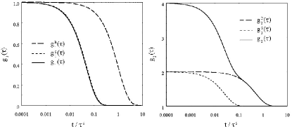
which, noticing that $N^{2}\left\langle u_{i}^{*}(t)u_{i}(t)\right\rangle^{2}=\left\langle I(t)\right\rangle^{2}$, yields the important Siegert relation:

$$g_{2}(\tau)=1+|g_{1}(\tau)|^{2}.$$ (18)

Hence, for a random source, $g_{2}(\tau)$ does not yield any additional information, and can be directly obtained from $g_{1}(\tau)$; in particular, for a collision-broadened thermal source $g_{2}(\tau)=1+\exp(-2|\tau|/\tau_{c})$. Nevertheless, the distinctive difference in the long-time asymptotic behavior between $g_{2}(\tau)$ and $g_{1}(\tau)$ yields, as we shall see, a crucial advantage for intensity correlation techniques.

II Dynamic Light Scattering (Intensity Correlation Spectroscopy)

The most popular optical correlation technique in colloid science is Dynamic Light Scattering, which I shall also call “Intensity Correlation Spectroscopy”, a denomination that captures much better, as we shall see, the essence of the method. This short presentation is mostly meant to stress those fundamentals of the technique that are essential to grasp the more recent advancement we shall later discuss. For the same reason, we shall just discuss DLS from a system of non-interacting particles, referring to excellent books and reviewsBerne and Pecora (1976); Chu (1991); Han and Akcasu (2011); Pusey (1977, 2002) for a more comprehensive treatment.

To spot the key feature of an intensity correlation measurement, let us make a comparison with a simple spectroscopic or interferometric experiment, where the signal is related to the spectrum $E(\omega)$, and therefore to the field time correlation function of the source, which in our case is the scattering volume. To select a given frequency, we have to insert a filter (such as a monochromator) on the optical path, and then detect the signal at the selected frequency. The basic strategy of DLS is simply moving the filter after the detector, so that the photocurrent output $i(t)$ of the detector, instead of the optical signal, is filtered. Any optical detectors is necessarily quadratic, namely, it detects a signal proportional to the time–averaged intensity $I(t)=\overline{E^{*}(t)E(t)}$: hence, by using a filter whose central frequency can be swept through a given range, the power spectrum of the signal can be obtained. Because of Wiener–Kintchine theorem, an equivalent procedure is measuring the time correlation function of $i(t)$, which is directly related to $\left\langle I(t)I(t+\tau)\right\rangle$. Whatever the choice, we shall see that operating on the photocurrent is a winning strategy for a basic reason: at variance with field correlation spectroscopy or interferometry the spectral bandwidth $\Delta\omega_{s}$ (or the correlation time $\tau_{s}$) of the source illuminating the scattering volume poses no limitation to the measurements, even when the spectral bandwidth of the scattered field $\Delta\omega\ll\Delta\omega_{s}$ (corresponding to a correlation time $\tau\gg\tau_{s}$). The first approach, based on using a spectrum analyzer, was mostly used at the dawn of DLS. The invention of the digital correlator (once a complex dedicated instrument, now just a PC data acquisition board), which allows to work in the time domain, has however been crucial to make DLS the spectroscopic method with the highest resolving power ever devised.

II.1 Time-dynamics of the scattered field

In a scattering experiment, the linear dimension of the scattering volume $V$ is usually much larger than the range $\xi$ of the structural and hydrodynamic correlations of the systems, even when the latter extend over large spatial scales compared to the particle size. Hence, $V$ can ideally be split into volume elements $\delta V$ satisfying $\xi^{3}\ll\delta V\ll V$. Consequently, $V$ can be regarded as a random source, where these uncorrelated volumes $\delta V$ play the role of “elementary emitters”. We may then expect the scattered field and intensity to display, respectively, a gaussian and an exponential statistics, and the time correlation functions of $E_{s}$ and $I_{s}$ to be dictated by the temporal correlation of the field emitted by a single elementary emitter, which will be related to the particle dynamics in $\delta V$. There are however a couple of warnings. First, the total scattered field has a gaussian statistics only provided that the field scattered by each single emitter is fully fluctuating in phase and/or amplitude. However, this is not true for many systems of interest in colloid science, such as glasses and gels: we shall comment on these “nonergodic” systems shortly. Second, the Siegert relation connecting field and intensity correlations is violated when the number $N$ of particles in $V$ is very small, which may be the case when performing measurements on very diluted suspensions under a microscope, if the coherence area of the illuminating source is small. In this case, by retaining the terms of order $1/N$ in Eq. (17), one can show that Eq. (18) contains an additional a number fluctuation term:

$$g_{2}(\tau)=1+|g_{1}(\tau)|^{2}+\frac{\left\langle\delta N(0)\delta N(\tau)\right\rangle}{\left\langle N\right\rangle^{2}},$$ (19)

where $\delta N(\tau)=N(\tau)-\left\langle N\right\rangle$ decays on a time scale comparable to the time it takes for a particle to move across the scattering volume.

The field scattered by a particle suspension can be written as

$$E_{s}(\mathbf{q},t)=E_{0}\sum_{i}b_{i}(\mathbf{q},t)\mathrm{e}^{{\rm i}\mathbf{q}\cdot\mathbf{r}_{i}(t)}.$$ (20)

If particles are all identical, and provided that the scattering amplitudes do not depend on time (which holds true for optically isotropic particles), the normalized field correlation function is then given by

$$g_{1}(q,\tau)=\frac{\left\langle E^{*}_{s}(\mathbf{q},0)E_{s}(\mathbf{q},\tau)\right\rangle}{|E_{s}(0)|^{2}}=F(q,\tau)\mathrm{e}^{-{\rm i}\omega\tau}$$

where we have defined the intermediate scattering function (ISF)

$$F(q,\tau)=\left\langle\sum_{i,j}\mathrm{e}^{-{\rm i}\mathbf{q}\cdot[\mathbf{r}_{i}(0)-\mathbf{r}_{j}(\tau)]}\right\rangle,$$ (21)

which is nothing but the FT (in frequency) of the dynamic structure factor $S(q,\omega)$ measured in quasi-elastic neutron scattering experiments. Neglecting interactions amounts of course to assume that the position of different particles are uncorrelated, so $g_{1}(q,\tau)$ is proportional to the self ISF

$$F_{s}(q,\tau)=\left\langle\exp[{\rm i}\mathbf{q}\cdot\Delta\mathbf{r}(\tau)]\right\rangle$$ (22)

where $\Delta\mathbf{r}(\tau)=\mathbf{r}(\tau)-\mathbf{r}(0)$. Therefore, $F_{s}(q,\tau)$ is the average value of $\exp[{\rm i}\mathbf{q}\cdot\Delta\mathbf{r}(\tau)]$ over the probability distribution $p(\Delta r,\tau)$ of the particle displacement in a time $\tau$. Note that, as a matter of fact, $\mathbf{q}\cdot\Delta\mathbf{r}$ is just the component $\Delta r_{q}$ of the particle displacement in the direction of the wave-vector $\mathbf{q}$. Hence, $F_{s}(q,\tau)$ can be seen as the Fourier transform $\mathscr{F}[p(\Delta r_{q},\tau)]$, which is the characteristic function of $p(\Delta r_{q},\tau)$. Given the characteristic function, all the moments of a probability distribution are easily calculated. For instance, the mean square particle displacement along $\mathbf{q}$ is given by

$$\left\langle\Delta^{2}r_{q}(\tau)\right\rangle=-\left[\frac{\partial g_{1}(q,\tau)}{\partial q^{2}}\right]_{q=0}$$ (23)

II.2 Time-correlation of the field scattered by Brownian particles

The simplest model of a freely–diffusing Brownian particle is that of a mathematical random walk. In one dimension, the particle motion is seen as a sequences of random “steps” $x_{i}$ along the positive or negative direction, so that $\left\langle x_{i}\right\rangle=0$ and, if we assume the steps to be uncorrelated $\left\langle x_{i}x_{j}\right\rangle=\left\langle x_{i}^{2}\right\rangle\delta_{ij}=\Delta^{2}\delta_{ij}$. Then, because of the Central Limit Theorem, the total displacement $x=\sum_{i=1}^{N}x_{i}$ for a large number $N$ of steps is a gaussian random variable with $\left\langle x\right\rangle=0$ and $\sigma_{x}^{2}=\left\langle x^{2}\right\rangle=N\Delta^{2}$. This corresponds, in a continuum description, to a diffusion process with a diffusion coefficient $D=\Delta^{2}/2\Delta t$, where $\Delta t$ is the time it takes for a step. Generalizing to 3D, the particle mean square displacement is then given by $\left\langle\mathbf{r}^{2}(t)\right\rangle=6Dt$, where, because of the celebrated Einstein’s relation, the diffusion coefficient is related to the hydrodynamic friction coefficient $\zeta$ by $D=k_{B}T/\zeta$ .

For $t\rightarrow 0$, the random walk model yields however a rather unphysical result, because the particle velocity diverges as $t^{-1/2}$. A more consistent description is obtained from the Langevin equation,Kubo et al. (1993) whose solution shows that the particle motion becomes diffusive only after the hydrodynamic relaxation time $\tau_{B}=m/\zeta$, where $m$ is the particle mass, which is the decay time of the velocity time-correlation function. It is also useful to note that the diffusion coefficient is just the time integral of the latter

$$D=\frac{1}{3}\int_{0}^{\infty}\!\!\!\left\langle\mathbf{v}(0)\cdot\mathbf{v}(t)\right\rangle\mathrm{d}t$$ (24)

For $t\gg\tau_{B}$, the probability for a particle to be in $\mathbf{r}$ if it was in the origin at $t=0$ is then a gaussian. Note however that we need only the component of the displacement in direction of $\mathbf{q}$ (which can in fact be taken as the $x$ axis), hence $p(\Delta r_{q},\tau)$ is a gaussian with $\left\langle\Delta r_{q}\right\rangle=0$ and variance $\sigma^{2}=2D\tau$. Being the characteristic function of a gaussian centered on the origin, $F_{s}(q,t)$ is itself a gaussian in $q$ with variance $1/\sigma^{2}=(2D\tau)^{-1}$, $F_{s}(q,\tau)=\exp(-Dtq^{2})$. Then as a function of $\tau$, the ISF decays exponentially with a rate $\Gamma=Dq^{2}$. The field and (because of the Siegert relation) the intensity correlation functions are given by

$$\left\{\begin{array}[]{l}g_{1}(\tau)=\exp(-{\rm i}\omega t)\exp(-\Gamma\tau)\\ g_{2}(\tau)=1+\exp(-2\Gamma\tau).\\ \end{array}\right.$$ (25)

II.3 DLS, the ultimate spectroscopy

Brownian motion gives then rise to a spectral broadening $\Gamma=Dq^{2}$ that, because $D$ is related to the particle radius, should allow for particle sizing. The problem, however, is that these spectral broadenings are extremely small, because colloidal diffusion is extremely slow: for instance, expressing its radius $R$ in nanometers, a spherical particle in water at $20^{\circ}$C has $D\simeq(2.15/R)\times 10^{-6}\mathrm{\,cm^{2}/s}$. Since the largest accessible $q$-values in light scattering are about $3\times 10^{5}\mathrm{\,cm^{-1}}$, even for a small surfactant micelle with a radius $R=2\mathrm{\,nm}$ the spectral broadening is of the order of $0.1\mathrm{\,MHz}$, which is negligible compared to the bandwidth of a spectral lamp, or of a common laser with no longitudinal mode selection. For “usual” colloids with a size in the tenths of a micron range, the situation is obviously far worse. Measuring a spectral broadening that is much smaller than the source intrinsic bandwidth is of course extremely challenging: as a matter of fact, it is totally out of question for any spectroscopic method relying on field correlations.

Yet, things change dramatically if we consider intensity correlations. This is probability easier to see in the time domain. Assume that a source has a bandwidth $\Delta\omega_{s}$, hence a coherence length $\ell_{c}\simeq 2\pi c/\Delta\omega$. If the scattering volume has linear dimensions $\ell=(V_{s})^{1/3}\ll\ell_{c}$, which is usually the case, each point in $V_{s}$ basically “sees” the same incident field. Hence, we can write $\mathbf{E}_{s}(q,t)=B(q,t)\mathbf{E}_{0}(t)$, where $\mathbf{E}_{0}(t)$ is the incident field and $B(q,t)=\sum_{i}b_{i}(q)\exp[{\rm i}\mathbf{q}\cdot\mathbf{r}_{i}(t)]$ the total scattering amplitude. However, $\mathbf{E}_{0}(t)$ and $B(q,t)$ are clearly independent random variables, so we have: $\left\langle B^{*}(q,0)E^{*}_{0}(0)B(q,\tau)E_{0}(\tau)\right\rangle=\left\langle B^{*}(q,0)B(q,\tau)\right\rangle\left\langle E^{*}_{0}(0)E_{0}(\tau)\right\rangle.$ Hence, the field correlation function factorizes as

$$g_{1}(q,\tau)=g_{1}^{S}(\tau)g_{1}^{B}(q,\tau)$$

where $g_{1}^{S}(\tau)$ is the time correlation function of the source and $g_{1}^{B}(q,\tau)$ is the sample correlation function due to particle Brownian motion. Since $g_{1}^{S}(\tau)$ decays to zero on the correlation time $\tau_{c}$ of the source, which is far shorter than the Brownian correlation time, there is no way to follow the decay of $g_{1}^{B}$. Consider however the intensity correlation function. Again, we can write

$$g_{2}(q,\tau)=g_{2}^{S}(\tau)g_{2}^{B}(q,\tau)$$

Yet, in this case, for $\tau\gg\tau_{c}$, $g_{2}^{S}(\tau)$ decays to one, and we have:

$$g_{2}(q,\tau)\underset{t\gg\tau_{c}}{\longrightarrow}g_{2}^{B}(q,\tau)$$ (26)

which is exactly what we want to measure.

Figure 1: Behavior of the field (left) and intensity (right) correlation functions, using a temporally partial coherent thermal source with $\tau_{c}^{S}=0.05\tau_{c}^{B}$.

In other words, we actually want to avoid using a source with a very long coherence time, for we need $\tau_{c}$ to be much shorter than the physical fluctuation time of the sample.

Of course, using single longitudinal mode lasers $g_{2}^{S}\equiv 1$, even if the effective laser bandwidth is not negligible, because the spectral broadening is due to pure phase fluctuations. The latter, however, still affect $g_{1}(\tau)$, thus hampering spectroscopic and interferometric measurements. Quantitatively,Pusey (1977) one finds that the scattered field is not gaussian, so that, in terms of the full correlation functions $g_{2}(q,\tau)\neq 1+|g_{1}(q,t)|^{2}$; yet, $g_{2}(\tau)=1+|g_{1}^{B}(q,t)|^{2}$, thus intensity correlation measurements still yield what is needed. Even if useful, using single–mode lasers in DLS is not at all compulsory, so much that the first attempts to study Brownian motion by analyzing the intensity fluctuations of speckle patterns were performed by Raman using a conventional mercury-arc lamp.Raman (1959) Hence, lasers are not used in DLS setups because of they are particularly monochromatic but, as we shall shortly see, just for practical reasons related to their unique spatial coherence properties.

In the frequency domain, we can see that the “magic” of intensity correlation comes from the fact that doing DLS is like playing a kind of “optical radio”. To broadcast an audio signal $v_{s}=f(t)$ we can for instance modulate the amplitude of a carrier wave at a radio frequency $\omega_{c}$ much larger than the frequency components of $f(t)$:

$$v(t)=A[1+mf(t)]\cos\omega_{c}t.$$

Then, to “decode” the signal, we use again a quadratic detector, which basically consist of a rectifier (a simple galena crystal in the first radios, a diode later). Suppose for simplicity that we wish to transmit a simple sinusoidal signal $\cos\omega_{m}t$, with $\omega_{m}\ll\omega_{c}$. Before the rectifier, the broadcast field is:

$$v(t)=A\cos\omega_{c}t+\frac{mA}{2}[\cos(\omega_{c}+\omega_{m})t+\cos(\omega_{c}-\omega_{m})t].$$

This contains, besides the original carrier frequency, two symmetric sidebands with $\Delta\omega=\pm\omega_{m}$ but, because $\Delta\omega\ll\omega_{c}$, no resonant filter can resolve them. After the rectifier, supposing that the modulation depth $m$ is small, we have:

$$v^{2}(t)\simeq\frac{A^{2}}{2}[1+\cos 2\omega_{c}t+m\cos(2\omega_{c}\pm\omega_{m})t]+mA^{2}\cos\omega_{m}t,$$

namely, besides a zero–frequency component and three components at radio-frequency (RF), we have obtained a signal at the modulation frequency that can be extracted with a low-pass filter. This strategy, which is called homodyne detection (the signal is “mixed with itself”), is again the result of using a quadratic detector. In DLS, the photodetector plays a role quite similar to the galena crystal, with $B(q,t)$ as modulating signal, although in the form $f(t)v_{c}(t)$ instead of [$1+mf(t)]v_{c}(t)$. The net effect of the “self–beating” of the scattered field on the quadratic detector is reconstructing a copy of the spectrum of $B(q,t)$ in baseband, but with all frequencies doubled.

II.4 Spatial coherence requirements in DLS

Intensity correlation measurements have several requirements in terms of spatial coherence for what concerns both the illuminating source and the detection scheme. Maximizing the DLS signal requires indeed to illuminate the scattering volume with a spatially coherent beam. Yet, we have seen that a source of area $A$ emits a spatially coherent field only within a solid angle $\Delta\Omega\simeq\lambda^{2}/A$: the useful emitted power is then just the amount contained in $\Delta\Omega$, namely, $P=SL\Delta\Omega$, where $L$, the power emitted per unit area and solid angle, is the radiance of the source (sometimes also called “brightness”, or “brilliance”). The crucial difference between a laser and a spectral lamp is actually its enormously higher spatial coherence, which is strictly related to its directionality. In fact, a gaussian beam emitted by a laser is perfectly coherent over its whole section, and diverges with the diffraction angle $\Delta\Omega=\lambda^{2}/w_{0}^{2}$, where $w_{0}$ is the minimum beam–spot size. The section of the emitted beam can therefore be regarded as a “speckle” emitted by a source of size $w_{0}$; a source, however, that emits all its power on a single speckle. It is actually their high brilliance that make lasers practically indispensable in DLS.

Let us now consider detection. The scattering volume behaves as a random source, with a size that is just the projection perpendicular to $\mathbf{q}$ of the illuminated volume. As a consequence, there is no advantage in using a detector with an area $A$ larger than a coherence area of this source. Namely, increasing the detector area beyond the size of the speckles made by the scattered field increases the detected power, but this additional power is of no use, for different speckles are uncorrelated. If the number $N=A/A_{c}$ of collected speckles is large, intensity fluctuations will grow just as $\sigma(I)\sim N^{1/2}$ (it is a Poisson statistics). Hence $g_{2}(0)-g_{2}(\infty)=\sigma^{2}(I)/\left\langle I\right\rangle^{2}\sim N^{-1},$ so we just loose contrast. For a generic value of $N$, one can actually write a “corrected” Siegert relation of the kind $g_{2}(\tau)=1+f(N)|g_{1}(\tau)|^{2}$, where the spatial coherence factor $f(N)$ can be approximately written as $f(N)\simeq(1+N)^{-1}$. To get a high contrast (a “good intercept”, in the jargon of DLS) , the detector aperture should be considerably smaller then a coherence area.

In the earliest schemes of a DLS apparatus, the angular extent of the scattered light reaching the photodetector was limited by means of two pinholes aligned along the selected scattering direction. However, a much more efficient detection scheme, which consists in forming by a lens an image of the scattering volume on a slit that can be closed or opened by micrometers to select a single speckle, was soon adopted. The real novelty is that the effective size of speckle on the slits can be tuned by stopping–down the lens with an iris diaphragm, because the image of a speckle gets convoluted with the lens pupil, so that by reducing the lens aperture the size of a coherence area on the image plane increases.Goodman (2005) We shall return to this idea of performing a “spatial coarse-graining” on the image plane in section IV. With these “traditional” detection schemes it is however very hard to reach a condition close to the “ideal” contrast $g_{2}(0)-g_{2}(\infty)=1$, which is conversely ensured by novel detection schemes using single-mode fibers that have become widespread in the last two decades. Understanding fiber detection requires however to forget all about “geometrical” arguments: neither the size of the fiber to be used, nor the distance of its opening from the sample, have indeed anything to do with the speckle size. Rather, an optical fiber has to be regarded as an “antenna”, which can resonate only on well-defined proper “modes”. A monomode fiber, in particular, allows for a single propagating mode, whose spatial structure is very similar to the fundamental transversal mode of a laser and display therefore full spatial coherence. The field detected by such a fiber is nothing but the projection (in the full mathematical sense) of the scattered field on the single fiber mode. The amplitude of the field collected by the fiber can vary by changing the size of the scattering volume or of the fiber core but, because of the full spatial coherence of the fiber mode, the field and intensity correlation functions always show full contrast, with values $g_{1}(0)=1$ and $g_{2}(0)=2$ at zero delay. One can show that the amplitude of the projected component can be maximized by matching the angular aperture of a speckle with the acceptance angle of the fiber. Besides being much simpler both conceptually and practically, fibers receivers present another very interested feature: if a laser beam is fed into the fiber from the opposite terminal (the one usually bringing the collected light to the photodetector) and launched towards the scattering cell from the receiver input, its spatial intersection with the incident beam allows to precisely define the scattering volume. By this trick, optical alignment, which is time–consuming in traditional DLS setups, becomes much simpler.Rička (1993)

II.5 Heterodyne detection and Doppler velocimetry

In radio engineering, homodyne detection has the disadvantage of generating a signal at $\omega_{m}$ which is proportional to the (generally weak) amplitude of the carrier wave detected by an aerial. Radios became much more efficient with the development of the “heterodyne” receiver, where the signal power is “pumped up” by mixing it with the signal $v_{L}(t)=A_{L}\cos\omega_{c}t$ from a local oscillator (LO) at the frequency of the carrier wave. Indeed, using a mixer that multiplies the incoming and LO signals, we get again the audio signal, but amplified by $v_{L}$:

$$V(t)=v(t)v_{L}(t)=AA_{L}(1+\cos\omega_{m}t)\cos^{2}\omega_{p}(t)=\{\mathrm{RFsignals}\}+AA_{L}\cos\omega_{m}t.$$

A very similar trick is used in heterodyne DLS, where the LO is simply a fraction of the incident beam (even simply a reflection from the cell windows) which “beats” with the scattered field on the photodetector. We have then

$$\left\langle I(0)I(\tau)\right\rangle^{HD}=\left\langle|E_{s}(0)+E_{L}(0)|^{2}|E_{s}(\tau)+E_{L}(\tau)|^{2}\right\rangle.$$

Neglecting fluctuations in the incident field (hence in $E_{L}$), observing that $E_{L}$ and $E_{s}$ are uncorrelated, and assuming that $|E_{L}|\gg|E_{s}|$ (which is almost unavoidable), one obtains after some calculation

$$g_{2}^{HD}(\tau)=1+k\mathrm{Re}[g_{1}(\tau)]$$ (27)

where $k=\left\langle I_{s}\right\rangle/I_{L}$. The important difference with respect to homodyne DLS is that, by heterodyning, we also detect the real part of oscillating terms of the form $\exp({\rm i}\omega\tau)$. Consider for instance a colloidal suspension in flow with a uniform velocity $\mathbf{v}$. The field correlation function can be evaluated by adding to the diffusion equation an advective term $\mathbf{v}\cdot\boldsymbol{\nabla}c$. Using the same method we have described earlier, one finds $g_{1}(q,\tau)=\exp({\rm i}\mathbf{q}\cdot\mathbf{v}\tau)\exp(-Dq^{2}\tau).$ The first phase term is totally “invisible” in homodyne detection, whereas:

$$g_{2}^{HD}(\tau)=1+k\exp(-Dq^{2}\tau)\cos(\mathbf{q}\cdot\mathbf{v}\tau)$$

Heterodyne detection is therefore at the roots of Laser Doppler Velocimetry, which allows to study hydrodynamic motion using particles as tracers, or the drift particle motion induced by an external field, such as in electrophoresis.

III Novel investigation methods based on intensity correlation

III.1 Multi–speckle DLS and Time-Resolved Correlation (TRC)

Colloidal gels and glasses are a class of materials of prominent interest characterized by an extremely low, quasi–arrested dynamics where each single particle performs a restricted motion around a fixed position. Because of the limited particle displacement, the scattered field can be written as the sum $\mathbf{E}_{s}(q,t)=\mathbf{E}_{f}(q,t)+\mathbf{E}_{c}(q)$ of a fully fluctuating component $\mathbf{E}_{f}(q,t)$ plus a time–independent contribution $\mathbf{E}_{c}(q)$. As a main consequence, $\mathbf{E}_{s}(q,t)$ is not anymore a fully–fluctuating gaussian random variable, and its statistical properties of are very different from those of the light scattered by free Brownian particles. The value of $\mathbf{E}_{c}(q)$ depends indeed on the specific configuration of the scatterers as seen from a given detection point, hence it is different from speckle to speckle because each coherence area comes from a unique combination of the phases of the individual fields scattered by each particle. Therefore, while evaluating the ensemble average of the scattered field over many speckles we get $\left\langle\mathbf{E}_{s}(q,t)\right\rangle_{e}=0$, the time average of $E_{s}(q,t)$ does not vanish, but is rather given by $\left\langle\mathbf{E}_{s}(q,t)\right\rangle_{t}=\mathbf{E}_{c}(q)$. Retrieving sound structural information by DLS on gels and glasses requires then to measure ensemble–averaged correlation functions. The latter can be of course obtained with a “brute force” method by very slowly displacing or rotating the cell between distinct acquisitions of $g_{2}(t)$, so that the detector is sequentially illuminated by many independent speckles. A different and far less time–consuming strategy was however proposed by Pusey and van Megen, who showed that the correct, ensemble-averaged correlation function may be reconstructed from the intensity correlation function measured in a single run on a fixed speckle, provided that the ensemble–average of just the static intensity $\left\langle I\right\rangle_{E}$ is carefully measured. The correct intensity correlation function is obtained from the single-run $g_{2}(\tau)$ and the ratio $\left\langle I\right\rangle_{t}/\left\langle I\right\rangle_{E}$ with a well–defined, although non trivial, correction scheme.Pusey and van Megen (1989)

Investigating “non-ergodic” media by traditional DLS is anyway laborious. Luckily, we can actually take advantage from the very slow dynamics of colloidal gels and glasses. In fact, neither a fast detectors as a photomultiplier, nor a real–time digital correlator are needed: a digital camera with a moderately fast data acquisition and transfer rate fully suffices, and the calculation of $g_{2}$ can still be made in real time via software. CCD and CMOS cameras are moreover multi-pixel devices, where each pixel acts as a detector, hence, in principle, we have a way to perform DLS measurements simultaneously on a vary large number of speckles. The outcome of such a multi-speckle experiment is a series of speckle images, where the intensity for each pixel $p$ and time $t$ is recorded. The intensity correlation function is then obtained as

$$g_{2}(\tau)=\left\langle\frac{\left\langle I_{p}(t)I_{p}(t+\tau)\right\rangle_{p}}{\left\langle I_{p}(t)\right\rangle_{p}\left\langle I_{p}(t+\tau)\right\rangle_{p}}\right\rangle_{t}$$

where $\left\langle\cdots\right\rangle_{t}$ is a time average, whereas $\left\langle\cdots\right\rangle_{p}$ denotes an average over an appropriate set of pixels corresponding to the same $q$-value. Because of the pre–averaging over many pixels, yielding very smooth data, multi–speckle detection yields a tremendous reduction of measurement time.

Multi–speckle methods are also ideal for investigating systems displaying heterogeneous temporal dynamics in glasses, foams, and a variety of jammed systems that often evolve in time through intermittent rearrangements. This is the principle of the Time–Resolved Correlation (TRC) technique,Cipelletti et al. (2003); Duri et al. (2005) where the change of the sample configuration is obtained by calculating the degree of intensity correlation between pairs of images taken at time $t$ and $t+\tau$, which explicitly depends on $t$

$$c_{I}(t,\tau)=\frac{\left\langle I_{p}(t)I_{p}(t+\tau)\right\rangle_{p}}{\left\langle I_{p}(t)\right\rangle_{p}\left\langle I_{p}(t+\tau)\right\rangle_{p}}-1.$$

The amplitude of the fluctuations in the temporal dynamics can then be quantified by the variance $\chi(\tau)=\left\langle c^{2}_{I}(t,\tau)\right\rangle-\left\langle c_{I}(t,\tau)\right\rangle^{2}$, which is directly related to the so-called dynamical susceptibility $\chi_{4}$ used to characterize dynamic heterogeneity in computer simulations of the glassy state. In the last section we will see that an extension of TRC, allowing to resolve $g_{2}(\tau)$ both in time and space, provides a basic link between scattering and imaging.

III.2 Near Field Scattering (NFS)

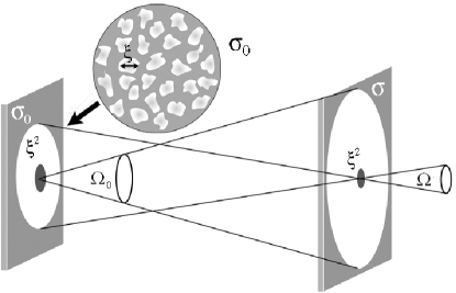
Because the scattered intensity has (for ergodic media) an exponential distribution with $\left\langle I^{2}\right\rangle=\left\langle I\right\rangle$, Eq. (15) basically states that the size of a speckle is just fixed by the geometry of the scattering volume, and does not contain any information about the physical mechanisms that produce scattering (see section I.2). This is a consequence of the VCZ theorem, which is however strictly valid only when the source is not spatially correlated. In fact, it is definitely not true for by a “structured source”, by which we mean a sample scattering light because of the presence of correlated regions of size $\xi\gtrsim\lambda$, due for instance to an inhomogeneous refractive index distribution.Giglio et al. (2000) For example consider, as in Fig. 2a, the scattering pattern generated on a close-by plane at distance $z$ from the cell by a suspension of colloidal particles contained in a thin cell, and illuminated with a beam spot of diameter $D$. Particles with a size $\xi\gtrsim\lambda$ scatter light mostly within a cone of angular aperture $\varphi\simeq\lambda/\xi$ (which, for very large particles, coincides with the angular aperture of their diffraction pattern). By reciprocity, light can reach a given point $P$ on the observation plane only from a region of size $d\simeq z\varphi$. Hence, $P$ sees an “effective” source with a size that, provided that $z<z_{c}=D\xi/\lambda$, is smaller than $D$. Rather surprisingly, the speckles generated by such a source have a typical dimension

$$\frac{\lambda}{d}z=\lambda\left(\frac{\xi}{\lambda z}\right)z=\xi.$$

The statistical size of a near–field speckle (which according to the VCZ theorem should vanish for $z\rightarrow 0$) is therefore of the order of the particle size.

Figure 2: Speckles in near field (a) and sketch of a NFS experiment (b).

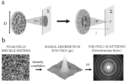
More quantitatively, it turns out that, for a structured source with a generic mass distribution, the intensity correlation function of the scattered light in the near–field is proportional to the radial distribution function $g(r)$, which yields, for non-interacting scatterers with a finite size, the average value for the speckle size we found with the former qualitative argument.Giglio et al. (2001) The intensity distribution $I(q)$ measured in the usual far–field scattering experiments, which is conversely proportional to the structure factor of the sample, can then also be obtained by evaluating the power spectrum of the intensity on a near field plane. These conclusions are fully confirmed by a reassessment of the VCZ theorem for a source with finite spatial correlation, which leads to conclude that, within the so-called “deep Fresnel region” (DFR) $z<z_{c}$, corresponding to large Fresnel numbers, the field correlation function is actually invariant upon propagation and approximately equal to that on the source plane, so the speckles retain the same size all along this region. For $z\gg z_{c}$, conversely, the source basically act as a collection of $\delta$-correlated emitters, and the standard VCZ theorem yields a good approximation for the mutual intensity on the observation plane.Cerbino (2007)

This Near-Field Scattering (NFS) technique present several advantages with respect to traditional methods to measure small-angle scattering, in particular when made using a heterodyne detection scheme, which just consists in letting the scattered field to “beat” with the transmitted beam, without blocking the latter:Giglio et al. (2001) in this configuration it requires indeed an extremely simple optical setup, in principle just a multi–pixel detector placed on the near-field observation plane. Of course, the speckle size should not be much smaller than the size of a pixel of the sensor, since we would otherwise average over many uncorrelated speckles, loosing contrast. However, if this condition is not met, the speckles can be magnified using a microscope objective: actually, the speckle size on the image plane depends only on the numerical aperture NA of the objective, and can be enlarged at will by reducing the latter. This trick of magnifying speckles by just stopping-down the imaging optics, is in fact similar to what is done in DLS detections by closing the diaphragm of the lens that images the sample volume on the slits. A second important advantage is that, because the scattered and transmitted beams are perfectly superimposed, NFS is an ideal heterodyne method that provides an absolute measure of the scattering cross sections, since the strength of the local oscillator is exactly known. An example of NFS experiment, made in our lab to obtain the form factor of very diluted polystyrene particles, in shown in Fig. 2b.

III.3 NFS velocimetry

Besides providing a simple and efficient tool to obtain the structure factor of a suspension at very small angles, heterodyne NFS can be used as a very accurate technique to measure the local motion in a fluid, using colloidal particles as “tracers” like in Particle Imaging Velocimetry (PIVAdrian (1991)). In a PIV measurement, a fluid containing tracer particles is illuminated by a thin sheet of light and imaged in the perpendicular direction. By measuring the tracer displacement between two closely spaced times, the two-dimensional in-plane velocity of the fluid is recovered, whereas a full 3-D reconstruction of the field profile can be obtained by holographic methods.Barnhart et al. (1994) Of course, tracking individual particles requires the latter to be large enough to be imaged, namely, the particle size must be larger than the resolution limit of the imaging system. This is usually acceptable when studying macroscopic hydrodynamics flow, but may raise several problems when dealing with flow around very small structures, which is often the case in microfluidic experiments. Suppose however that we perform a NFS measurement on a moving suspension, namely from particles that, besides performing Brownian motion, are transported by the suspending fluid. As we discussed, a detector placed on a plane $P$ within the deep-Fresnel region, or on the plane where $P$ is imaged by a microscope objective, collects light from a region $D^{*}\ll D$, where $D^{*}$ is respectively determined by the scattering cone of the scatterers or by the NA of objective. If all scatterers are rigidly displaced transversally to the optical axis, the speckle field just displaced accordingly, with no relative change in the speckle position. Note that this one-to-one mapping between particle motions and speckles displacement works only in NFS conditions: upon particle motions, the far–field speckle pattern remains stationary, simply fluctuating in time due to Brownian motion, because each speckle is the result of contributions arriving from the whole illuminated region $D$.

Hence, a statistical analysis of speckle patterns taken at different times allows to recover the tracer motion, and map the fluid velocity profile.Alaimo et al. (2006) This can either be done by measuring the cross-correlation function between two subsequent patterns, or from observing the effects of the tracer motion on the far–field scattered intensity reconstructed by a Fourier transform. Writing the total heterodyne intensity as $I(\mathbf{r},t)=I_{0}+\delta I_{t}(\mathbf{r})$, where $\delta I_{t}(\mathbf{r})=2\mathrm{Re}[E_{t}E_{s}^{*}(t)]$, and assuming that the fluid embedding the tracers is moving at constant velocity $\mathbf{V}$, after a delay $\Delta t$ the fluctuating part becomes $\delta_{t+\Delta t}(\mathbf{r})$ = $\delta_{t}(\mathbf{r}-\Delta\mathbf{r})$, where $\Delta\mathbf{r}=\mathbf{V}\delta t$. Then, the cross-correlation of the speckle pattern between $t$ and $t+\Delta t$ is simply a “shifted version” of the signal at time $t$:

$$G_{\Delta t}(\mathbf{x})=\left\langle\delta I_{t}(\mathbf{r})\delta I_{t+\delta t}(\mathbf{r}+\mathbf{x})\right\rangle=\left\langle\delta I_{t}(\mathbf{r})\delta I_{t}(\mathbf{r}-\Delta\mathbf{r}+\mathbf{x})\right\rangle=G_{0}(\textbf{x}-\Delta\mathbf{r}).$$ (28)

In other words, the cross-correlation shows a pronounced peak located at $\mathbf{x}=\Delta\mathbf{r}$ that, for constant $\mathbf{V}$, shift linearly with time. For practical reasons, it is often more useful considering the autocorrelation of the difference signal

$$\delta I^{\prime}_{\Delta t}=I_{t+\Delta t}(\mathbf{r})-I_{t}(\mathbf{r})=\delta I_{t+\Delta t}(\mathbf{r})-\delta I_{t}(\mathbf{r}),$$

which is a zero-average fluctuating variable that does not require, to be evaluated, the subtraction of the time–independent background. In this case, one gets two symmetric correlation peaks.Alaimo et al. (2006) This alternative approach is also useful because, considering the FT of $\delta I^{\prime}_{\Delta t}$ and making use of the shift theorem, one easily finds that

$$\left|\mathscr{F}[\delta I^{\prime}_{\Delta t}]\right|^{2}=I(q)[1-\cos(\mathbf{q}\cdot\Delta\mathbf{r})].$$ (29)

Thus, particle motion shows up in the structure factor as a set of straight fringes perpendicular to $\mathbf{V}$, with a spacing $\Lambda=2\pi/|\mathbf{q}\cdot\mathbf{V}\Delta t|$ that narrows linearly in time.

III.4 The third dimension of the speckles

In section I.2 we have discussed the two-dimensional properties of the speckles, namely, what is the statistical distribution and characteristic “granularity” of the maculated pattern observed on a screen placed at a given distance from a random source. In fact, we have spoken of coherence areas: however, we may wonder whether speckles also have a “depth” along the direction of propagation, and how this depth depends on the distance from the source. To avoid confusion, we are referring here to a purely spatial longitudinal coherence for a monochromatic source (for a polychromatic source with finite bandwidth, there is an obvious longitudinal limit to extent of field correlations, which is given by the coherence length $\ell_{c}$). The longitudinal coherence of speckles is important in several novel techniques, such as speckle photography, interferometry, and holography, yet it has been the subject of relatively few theoretical investigations (for a review till 2007, see.Goodman (2007))

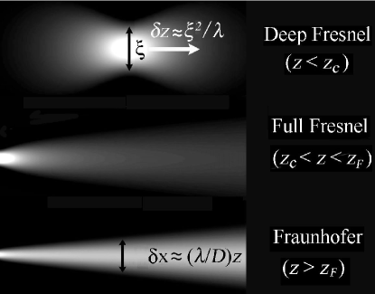
Without entering in the details of the analysis, we just quote here the main results obtained in novel approachesAlaimo (2006); Gatti et al. (2008) where the problem is carefully reconsidered in relation to the distance from the source: quite different properties of the 3-D speckles are indeed found depending on whether they are observed in the deep Fresnel region, in far-field Fraunhofer diffraction, or in the intermediate “full” Fresnel regime where the VCZ theorem already holds in the form given by Eq. (14) (see footnote References). Suppose that a random diffuser is illuminated by a laser beam focused on the diffuser to a spot size $D$ (so that the illuminating wavefront is flat). We shall also assume that the source is quasi–homogeneous, meaning by that that the spatial correlations of the diffuser extend over a typical size $\xi\ll D$. Then, the transitions between a different “morphology” of the 3-D speckles generated by the diffuser are marked by the distances $z_{c}=D\xi/\lambda$ and $z_{F}=D^{2}/\lambda$. Let us summarize the main aspects of these regimes.

“Deep” Fresnel region ($z<z_{c}\ll z_{F}$)

As already discussed, in this near–field region the trasverse coherence length $\delta x$ of the speckles does not depend on $z$ and coincides with $\xi$. Physically, the speckle pattern on a plane at distance $z$ can be pictures as made of luminous “spots” with an average size $\xi$, separated by a typical distance which is also of order $\xi$. The longitudinal coherence length $\delta z$ can be qualitatively found as follows. Since $z\ll z_{F}$, the beam wavefront is still approximately flat, namely, each speckle behaves like an aperture illuminated by a plane wave and broadens upon propagation just because of diffraction, with a characteristic diffraction angle $\vartheta_{d}\sim\lambda/\xi$. The longitudinal coherence length can be roughly evaluated as the distance where the diffraction patterns from two neighbor speckles starts to interfere. Hence $\delta z\simeq\xi/\vartheta_{d}\simeq\xi^{2}/\lambda$, which correctly estimates the value obtained from a rigorous approach. A 3-D speckle in near field can then pictured as a kind of “jelly bean” with a coherence volume of order $\xi^{2}\times(\xi^{2}/\lambda)=\xi^{4}/\lambda.$

Fraunhofer region ($z\gg z_{F}$)

As the distance from the source increases beyond $z_{c}$, we enter the region where the usual VCZ theorem holds. Here speckles grow in transverse size as $\delta x(z)\simeq\lambda z/D$, so they diffract at smaller and smaller angles $\vartheta_{d}\simeq\lambda/\delta x\simeq D/z$. On the other hand, the wavefront of the overall beam becomes progressively curved, so that each speckle “expands” as a spherical wave. In the Fraunhofer region, where the speckles have consistently expanded, the diffraction effects ruling speckle growth in the DFR becomes negligible, while the beam wavefront has a radius of curvature approximately equal to the distance $z$ from the source. Because of this curvature, two neighbor speckles of size $\delta x=z\lambda/D$ broaden and simultaneously spread apart at the same rate $\vartheta_{c}\simeq\delta x/z\simeq\lambda/D$. Hence, their “paths” do not cross any more, and each speckle preserves its own coherence in propagation (no “crosstalk” between the speckles). As a consequence, the 3-D geometrical shape of a speckle changes dramatically from a jelly bean to a pencil. Hence, in the Fraunhofer region, $\delta z\rightarrow\infty$.

“Full” Fresnel region $z_{c}<z<z_{F}$

We have seen that speckle growth is due to two distinct mechanisms: diffraction, dominating in the DFR, and expansion due to wavefront curvature, which is the sole mechanism operating in far–field. The distance from the source where the two contribution becomes comparable can be found by equating

$$\vartheta_{d}\simeq\vartheta_{c}\Longrightarrow\delta x\sim D\Longrightarrow z\simeq\frac{D^{2}}{\lambda}=z_{F}$$

Hence, in the “usual”, or “full” Fresnel region we are considering, both mechanisms are operating, and simple scaling arguments do not help. Nonetheless, we can qualitatively say that, as the distance from the source grows, the wavefront becomes curved and the speckles start to spread apart. Because of this, the diffraction patterns from two neighbor speckles take longer to interfere, and the coherence length becomes longer than the pure diffractive length $\delta x^{2}/\lambda$. Thus, a 3D-speckle in this region cans till be viewed a jelly beans, but sensibly elongated in the direction pointing away from the source.

A schematic view of the three regimes is shown in Fig. 3 (for a more quantitative description, seeGatti et al. (2008)). We recall, however, that all we have said refer to an ideal monochromatic source, whereas the longitudinal coherence of a polychromatic source is in any case be upper limited by $\ell_{c}=c\tau_{c}$.

Figure 3: Sketch of the longitudinal coherence profile of speckles from an ideal monochromatic sources in the deep Fresnel, Fresnel, and Fraunhofer regions.

IV Spatial coherence and imaging

In its simplest acceptation, imaging consist in producing, by means of optical elements like lenses or mirrors, a faithful copy of a planar section of an object onto another plane, apart from a change of scale (magnification). To what extent the copy we make can be really faithful is however limited not only by the “stigmatic” properties of the imaging system (for instance by the presence of geometrical aberrations), but also on diffraction effects, which set the resolution limit, and therefore the maximum useful magnification, of an imaging system. Hence, it is not surprising that, since the seminal investigation by Ernst Abbe, diffraction has been a fundamental tool to investigate image formation under a microscope. Yet, spatial coherence plays a primary role too, although this is usually marginally considered in introductory textbooks on microscopy (with the noticeable exception of a recent book by MertzMertz (2010)). To properly understand how a microscope really works requires however some basic concepts in Fourier optics and some additional results from statistical optics.Goodman (2005); Mertz (2010)

a) Angular spectrum

While investigating diffraction effects, it is usually possible to select a “main” propagation direction $z$ (the optical axis), and expanding a generic wavefront in terms of plane waves propagating with specific components of the wave-vector $\mathbf{k}$ along $x$ and $y$. This is done by decomposing the amplitude $U(x,y,z)$ of a monochromatic optical field with a partial inverse Fourier Transform along $x,y$ as:

$$U(x,y,z)=\int\mathrm{d}f_{x}\mathrm{d}f_{y}A(f_{x},f_{y},z)\mathrm{e}^{2\pi{\rm i}(f_{x}x+f_{y}y)},$$

where $f_{x}$ and $f_{y}$ are called spatial frequencies and

$$A(f_{x},f_{y},z)=\int\mathrm{d}x\mathrm{d}yU(x,y,z)\mathrm{e}^{-2\pi{\rm i}(f_{x}x+f_{y}y)}.$$

Spatial frequencies be given a simple geometric interpretation by expressing the amplitude of a simple plane wave in terms of the director cosines $(\alpha,\beta,\gamma)$ it makes with the axes $(x,y,z)$ as

$$P(x,y,z)=\exp[{\rm i}(2\pi/\lambda)(\alpha x+\beta y)]\exp[{\rm i}(2\pi/\lambda)\gamma z].$$

Thus, across the plane $z=0$, $\exp[2\pi{\rm i}(f_{x}x+f_{y}y)]$ may be seen as a plane wave traveling with director cosines $\alpha=\lambda f_{x}$, $\beta=\lambda f_{y}$. However, the director cosines are not independent, because $\gamma=\sqrt{1-\alpha^{2}-\gamma^{2}}.$ The physical meaning of this relation can be grasped by observing that $U(x,y,z)$ satisfies the Helmholtz equation $(\nabla^{2}+k^{2})U(\mathbf{r})=0$, with $k=2\pi/\lambda$. Hence, writing $A(\alpha,\beta,z)=\int\mathrm{d}x\mathrm{d}y\,U(x,y,z)\mathrm{e}^{-{\rm i}k(\alpha x+\beta y)}$, we have

$$\frac{\partial^{2}A(\alpha,\beta,z)}{\partial z^{2}}+k^{2}(1-\alpha^{2}-\beta^{2})A(\alpha,\beta,z)=0\Longrightarrow A(\alpha,\beta,z)=A(\alpha,\beta,0)\mathrm{e}^{{\rm i}k\gamma z}.$$

For $\alpha^{2}+\beta^{2}\leq 1$ ( $f_{x}^{2}+f_{y}^{2}\leq\lambda^{-2}$) $\gamma$ is real, hence propagation just amounts to a change of the relative phases of the components of the angular spectrum, because each wave travels a different distance between constant-$z$ planes, which brings in phase delays. Conversely, for $\alpha^{2}+\beta^{2}>1$ $\gamma$ is imaginary, and $\alpha$, $\beta$ cannot be regarded anymore as true direction cosines. Rather, we have an evanescent wave, whose amplitude decays as $\exp(-2\pi|\gamma|z)$ and becomes negligible as soon as $z$ is a few times $\lambda$. Wave propagation in free space can then be regarded as a “low–pass dispersive filter”, since only those spatial frequencies such as $f_{x}^{2}+f_{y}^{2}\leq\lambda^{-2}$ can propagate, with a phase shift that depends however on frequency.

b) Fourier–Transform properties of a lens

Suppose we illuminate with uniform amplitude $A$ a flat object, for instance a transparency transmitting an amplitude $U(x,y)=At(x,y)$, placed against a thin lens of focal length $f$. Then, if the object is much smaller than the lens aperture, so that we can neglect the effect of the finite size of the latter, the amplitude distribution $U_{f}(x,y)$ in the focal plane of the lens is the Fraunhofer diffraction pattern of the object transmittance $t(x,y)$, aside from a pure phase factor that does not change the intensity. The former phase factor exactly cancels out when the object is placed at a distance $f$ before the lens. In other words, the front and back focal planes of a lens are related by a FT or, as we shall say are reciprocal Fourier planes. Finally, is an object is placed before a thin lens at a distance $z_{1}$ then (except again for phase factors) an image of the object, inverted and magnified by the ratio $M=-z_{2}/z_{1}$, forms at a distance $z_{2}$ such that $z_{1}^{-1}+z_{2}^{-1}=f^{-1}$, which is of course the simple lens law from geometrical optics. Moreover, the back focus is exactly a Fourier plane for the object, so we can “manipulate” the image, for instance by “cutting out” some spatial frequencies or by selectively changing their relative phases. This “spatial filtering” technique, besides being at the roots of the whole field of optical communication, is fully exploited in phase–contrast microscopy. The effect of the lens pupil is very similar, since also the lens plane is (aside from a phase factor) a Fourier plane for the object. Hence, reducing the lens diameter $D$ (or better, its numerical aperture $NA=D/f$) corresponds to cut out the high-frequency Fourier components, in fact reducing the image resolution.

c) Aperture and field stops

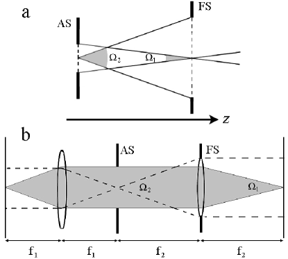
In free space, all spatial frequencies with $f_{x}^{2}+f_{y}^{2}\leq\lambda^{-2}$ propagate, whereas evanescent waves die out. When an optical signal is fed through a generic imaging system, however, there are further limitations to the spatial frequencies that can reach the image plane, because the finite size of the optical components limits the angular extent of the radiation emitted by the object that can propagate through the system. Crucial to the analysis of spatial coherence in an optical system are the concepts of aperture and field stops, which are defined as follows. Let first look at the optical system from the image plane, and find what is the aperture which most limits the incoming light: this is the aperture stop AS, or simply the “pupil” of the system. Now project of cone from the center of the aperture stop, and find what is the stop that limits its angular aperture: this is the field stop FS. For example, Fig. 4a, shows the aperture and field stops for a simple propagation between two diaphragms, whereas in the so–called $2f_{1}-2f_{2}$ lens system shown in Fig. 4b (a very convenient combination for spatial filtering) AS is the diaphragm placed in the common focus of the two lenses, while FS is the pupil of the lens that limits more the angular aperture.

Figure 4: Aperture and field stops for free propagation between two apertures (a) and for a $2f_{1}-2f_{2}$ lens system (b).

Partially–coherent sources

According to footnote References, the fundamental gaussian mode emitted by a laser has a far–field angular divergence $\theta\simeq\lambda/(\pi w_{0})$, where $w_{0}$ is the beam waist, which is the spread expected for a spatially coherent wavefront because of diffraction. For a partially coherent circular source of area $\sigma_{0}=\pi w_{0}^{2}$, which can be pictured as “speckle mosaic” made of $N_{c}\sim\sigma_{0}/\xi_{0}^{2}$ uncorrelated coherence regions of size $\xi_{0}$ (see figure 5), the divergence is found to be $N_{c}$ times larger.

Figure 5: Propagation of the spatial coherence for a partially–coherent source and étendue.

It is however interesting to investigate how the correlation length changes upon propagation. We have seen that, in the deep Fresnel region, the propagation of the spatial coherence is very different from what predicted by the VCZ theorem for a fully uncorrelated source. Here, however, we wish to find how a similar source behaves in far field, namely, in the Fraunhofer diffraction regime. Without entering into details, which involve rather tedious calculations, we just state the main result. In far field, the area $\sigma$ of the source and the correlation length $\xi$ grow upon propagation by a distance $z$ as

$$\left.\begin{array}[]{l}\sigma=\dfrac{(\lambda z)^{2}}{\xi_{0}^{2}}\vspace{3pt}\\ \xi^{2}=\dfrac{(\lambda z)^{2}}{\sigma_{0}}\\ \end{array}\right\}\Longrightarrow\frac{\sigma}{\xi^{2}}=\frac{\sigma_{0}}{\xi_{0}^{2}}.$$ (30)

Hence, the “expansion rate” of the source area is determined by the area of a coherence region and vice versa. It is therefore useful to define a quantity with the dimensions of an area called the étendue

$$G=\lambda^{2}\frac{\sigma}{\xi^{2}}.$$ (31)

which, because of Eq. (30), has the very important property of being conserved upon free–space propagation. Moreover, introducing as in Fig. 5 the solid angles $\Omega_{0}=\sigma/z^{2}$ and $\Omega=\sigma_{0}/z^{2}$, we can also write $G=\sigma_{0}\Omega_{0}=\sigma\Omega$. Physically, the étendue is a “combined extension” of the source, given by the the product of its area in the real space times its far–field diverging angle, which is related to the region in the Fourier space of the spatial frequencies that propagate from $\sigma$. For a uniform source, we can the write the total emitted power as the product $W=GL$ of the étendue times the radiance: since $W$ is of course fixed, the invariance of the étendue upon free–space propagation is equivalent to the conservation of the source brightness.

The étendue is however not conserved in the presence of limiting apertures. Suppose for instance that a fully coherent planer wavefront of infinite lateral extent impinges on the simple system in figure 4a, where the aperture stop AS limits the source size, while the field stop FS its angular divergence: it is easy to show that the effective étendue is limited to $G_{t}=A_{s}\Omega=A_{f}\Omega^{\prime}=A_{s}A_{f}/z^{2}$, where $A_{s}$ and $A_{f}$ are the areas of the aperture and field stop respectively. This is called the throughput of an optical system. Using the double–diaphragm setup in figure 4, we can actually increase the effective spatial coherence of a source: this happens whenever the solid angle subtended by FS is smaller than than $\Omega_{0}$ (we loose of course some power). This also helps to understand fiber–optic detection in DLS. A monomode optical fiber has by definition an étendue $G=\sigma_{f}\Omega_{f}=\lambda^{2}$ where $\sigma_{f}$ and $\Omega_{f}$ are the area of the fiber core and its solid acceptance angle. For a source of étendue $G$, the maximum power fed into the fiber is $W=W_{0}\sigma_{f}\Omega_{f}/G$. It is then easy to show that, for a monomode fiber collecting scattered radiation, $W$ coincides with the power scattered by the sample within one speckle.

IV.1 Microscope structure: coherence of illumination and resolution limit

Figure 6: Structure of a microscope with Köhler illumination. The illumination path consists of the collector lenses $L_{1}$ and $L_{2}$ that generate an image of the illumination source on the plane of the condenser, which focuses the light on the object plane. In the imaging path, the transmitted light is collected by an infinity–corrected objective and made parallel by the tube lens. The two conjugate sets of planes where the illumination source and the sample are in focus are shown by corresponding symbols.

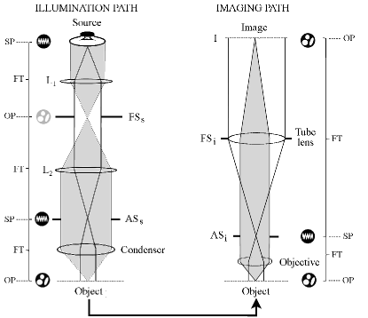
Fig. 5 shows the basic structure of an optical microscope using Köhler illumination. This setup provides a uniform illumination of the sample by placing the latter on the focal plane of the condenser, which is a conjugate Fourier plane for the illuminating lamp. As a matter of fact, in the configuration shown in Fig. 6 there are actually two sets of planes where the source $S$ and the object (sample) plane are, respectively, imaged. Set 1 is composed of the lamp filament, the source aperture stop $\mathrm{AS}_{s}$ at the front focal plane of the condenser, and the image aperture stop $\mathrm{AS}_{i}$ at the back focal plane of the objective. All these planes are Fourier planes for set 2, which comprises the field stop $\mathrm{FS}_{s}$ at the back focal plane of the collector lens $L_{1}$, the object plane where the sample is placed, and the image plane (in visual observation, the latter is further imaged by the eyepiece).

Understanding the reciprocal nature of these two sets of planes is crucial to describe the way a microscope works. In particular, it is important to stress that the size of the illumination source and its spatial coherence properties can be controlled independently. The former is simply tuned by opening or closing the diaphragm $\mathrm{AS}_{s}$. The field stop $\mathrm{FS}_{s}$ conversely controls the angular aperture of the light reaching the sample from a given point on the source plane. Since the latter lies on the focal plane of $L_{1}$, where we have the FT of the source, closing down $\mathrm{FS}_{s}$ corresponds to filtering the spatial frequencies of $S$ and therefore to tuning the spatial coherence properties of the source. By increasing the condenser aperture, the illuminating optics becomes more and more similar to a fully incoherent source, whereas by progressively stopping it down we approach the coherent illumination limit. From what we have seen in the previous section, the illumination on the object plane has then in general the form of a “speckle mosaic” similar to the one sketched in figure 5, where the speckle size $\xi$ is fixed by the condensed numerical aperture. In section V.2, we shall see how novel correlation methods in microscopy exploit this peculiar tunability of the spatial coherence of illumination.

The degree of spatial coherence of the illumination at the sample plane has noticeable effects on the resolving power of the microscope. For of a telescope with an objective of radius $w$, the determination of the resolving power is particularly simple, because two close-by stars we may wish to resolve behave as mutually incoherent point sources. Moreover, since the telescope is focused ai infinity, each one of them is imaged on the focal plane of the objective as an “Airy disk” (namely, the Fraunhofer diffraction pattern of a circular aperture) of diameter $d\simeq 0.6\lambda f/w$. A reasonable criterion for separation, suggested by Rayleigh, is that they are “barely resolved” if the center of the Airy disk of one star coincides with the first minimum of the second one, namely, if their angular separation is larger than $\vartheta_{min}\simeq 0.6\lambda/w$. For microscope, however, the problem is more complicated, first because this simple result from Fraunhofer diffraction holds only provided that ray propagation is paraxial, which is the case of a telescope but surely not of a microscope; second, because we are considering non self-luminous objects, hence the spatial coherence of the light generated at the object plane depend on the coherence of the illuminating source. Consider first the situation where the illumination is fully incoherent, which can be obtained for instance by opening up completely the field stop $\mathrm{FS}_{s}$ of the condenser. If we take a look to the “imaging path” to the right of figure 6, we can see that the spatial frequencies of the light produced at the object plane that can reach the image plane are basically limited by the aperture stop $\mathrm{AS}_{i}$. Since the object plane lies very close to the front focal plane of the objective, the maximum spatial frequency that enters the imaging path is determined by the numerical aperture of the latter $NA_{obj}=n\sin\vartheta$, where $\vartheta$ is the angle subtended by $\mathrm{AS}_{i}$ when viewed from the image plane, and $n$ is refractive index of the medium the objective is immersed in (which may not be air). It is then not hard to deduce that the Rayleigh limit is generalized by the celebrated Abbe criterion, stating that the minimal separation distance is:

$$\delta\simeq 1.22\frac{\lambda}{n\sin\vartheta}=1.22\,\frac{\lambda}{NA_{obj}},$$

For fully coherent illumination, however, things are quite different, even in the paraxial approximation, and the result depends on phase difference $\varphi$ of the illumination at the two point sources. Indeed, one finds that the situation is identical to the incoherent case only when the phases are in quadrature ($\varphi=\pi/2$), whereas, when the two sources are fully in phase ($\varphi=0$), the two Airy disks conversely merge into a single peak centered at $x=0$: thus, at the Rayleigh limit, they are not resolved at all. If the sources are in counter-phase ($\varphi=\pi$), however, at the Rayleigh limit they are fully separated, hence resolution actually doubles. Stating that coherent illumination is “worse” than incoherent illumination, as often made in elementary textbooks, is therefore incorrect. With coherent illumination, the resolution actually depends on the specific way we illuminate the object: whereas in a standard geometry two close-by points are usually illuminated with the same phase, with a suitable oblique illumination (a technique which has often been used in microscopy) one can obtain a counter–phase condition. Even with a standard illumination geometry, the best resolution is not obtained by increasing as much as possible the condenser aperture. A detailed calculation shows indeed that it is not worth increasing the condenser numerical aperture $NA_{con}$ to more than about $1.5NA_{obj}$, and that in these conditions the resolving power isBorn and Wolf (1997)

$$\delta\simeq 1.22\,\frac{\lambda}{NA_{obj}+NA_{con}}.$$ (32)

V Scattering and imaging: towards a joint venture

We have seen how statistical optics concepts can describe both DLS and imaging by a microscope. Yet, communication between these two worlds has been rather limited till a few years ago. The main reason is that the description of particle scattering necessarily requires a full 3-D treatment of the electromagnetic problem leading, even in the case of spherical particles, to the complicated Lorenz-Mie solution. On the other hand, most traditional microscopy problems can be discussed using the simpler language of diffraction, which is basically 2-D. Recent advancements in imaging, such as the development of confocal microscopy and of accurate particle–tracking methods, have led to investigate many aspects of imaging of 3-D objects, and to reconsider the relation between scattering and microscopy.

The latter is far from being trivial. It is not easy even to state when we can actually see under a microscope a particle made of a non-absorbing material and with a size much larger than the wavelength. If we regard them as two dimensional sources and just apply the basics of Fourier optics, the answer is simple: never. A non absorbing particle just modulates the phase of the illuminating radiation, and does not change its amplitude: in other words, they are phase diffractive elements, and the image of a phase element is again a phase element, with no intensity contrast.Goodman (2005) Cells and other optically transparent biological samples object are indeed practically invisible, except at their contour boundaries, but, as a matter of fact, large polystyrene particles can be seen under a microscope, even when they are right on focus. This must have therefore to do both with the 3D nature of the particles, and with the difference $n_{p}-n_{s}$ between the refractive indexes of the particle and of the solvent. In fact, particles of a size $a$ such that $|n_{p}-n_{s}|a/\lambda\ll 1$ (namely, Rayleigh-Gans scatterers) cannot be visualized at all, and the same is true for particles scattering in the so-called “anomalous diffraction” regime,C.van de Hulst (1957) where reflections and refractions at the particle/solvent interface can be neglected. A detailed analysis of the visibility problem for a generic scatterer is however still lacking. Scattering from non-absorbing objects is in any case rather weak, whatever their refractive index with the surrounding medium, hence a common way to increase their visibility is “de-focusing”, namely, focusing the objective on a plane outside the particle. However, it is worth noticing that, with this methods, evaluating particle size or interparticle distances is not trivial, and may lead to serious errors.Baumgartl and Bechinger (2005) In fact, quantifying how the imaging optics collects the intensity distribution generated on a generic plane from particles situated at various distances $z$ from it requires a full 3D treatment of the imaging process. In the simplest case of a Rayleigh–Gans scatterer, one finds that the intensity pattern consists of a central disk surrounded by a set of concentric fringes that get the coarser the farther is the particle from the plane $z=0$, and that a particle displacement at constant $z_{0}$ amounts to a rigid translation of this fringe pattern, similarly to what is observed in out-of-focus microscopy observations. A full discussion of 3D imaging can be found in Ref.Streibl (1985); Nemoto (1988).

For what follows it is also useful relating the scattering wave-vector $\mathbf{q}$ to its projection $\textbf{q}_{\shortparallel}$ on the observation plane $z=0$. Since in the paraxial approximation $q=2k\sin(\theta/2)\simeq k\theta$, where $\theta$ is the scattering angle, we have

$$q^{2}\simeq q_{\shortparallel}^{2}\left[1+\left(\frac{q_{\shortparallel}}{2k}\right)^{2}\right],$$ (33)

so that the perpendicular component of $\mathbf{q}$ is $q_{z}\simeq q_{\shortparallel}^{2}/2k$. The second term in square brackets is of order $\theta$, so it is negligible for small scattering angles. Notice however that, according to Eq. (33), the same $\mathbf{q}_{\shortparallel}$ vector may actually correspond, for two distinct wavelengths, to different $\mathbf{q}$ vectors. Nevertheless, it is not difficult to show that this effect is small as long as the difference in wavelength $\Delta\lambda\ll q_{\shortparallel}^{-1}$, which is of order $\lambda/\theta$: hence at small collection angles, the speckle patterns formed by different wavelengths superimpose.

V.1 Photon Correlation Imaging (PCI)

TRC is a very powerful method to investigate the heterogeneous and intermittent time–dynamics of restructuring processes in gels and glasses. However, glassy dynamics is also very heterogeneous in space, behaving very differently in different regions of the sample at equal time. Photon Correlation Imaging,Duri et al. (2009) a simple extension of TRC, allows to detect these spatial heterogeneities by means of measurements of space and time resolved correlation functions. With respect to the TRC scheme, the major change concerns the collection optics. Instead of collecting the light scattered in far–field, one forms an low-magnified image of the scattering volume onto a multi-pixel detector, using only the light scattered in a narrow cone centered around a well defined scattering angle. Of course, since the magnification $M$ is low, the scatterers themselves are not resolved, but a speckle pattern is visible, because we are actually collecting the light within all the depth of field of the imaging lens, hence also the near–field scattering from the sample. In fact, we can tune the size of the speckles by adjusting the NA of the imaging lens with an iris diaphragm, exactly as when, in heterodyne NFS, the near–field speckle pattern is magnified using an objective. In contrast to far field speckles that are formed by the light coming from the whole scattering volume, however, each speckle in a PCI experiment receives only the contribution of scatterers located in a small volume, centered about the corresponding object point in the sample. The linear size of this volume will be of order $(\lambda/Md)z$, where $d$ is the diameter of the lens pupil, and $z$ the lens-detector distance. As a result of the imaging geometry, the fluctuations of the intensity of a given speckle are thus related to the dynamics of a well localized, small portion of the illuminated sample. Hence, the local dynamics can be probed by dividing the image in “Regions of Interest” (RoI) which contains a sufficient number of speckles and measuring their time-fluctuations.

This method was developed to study slow or quasi–arrested systems, but it works also for free particles in Brownian motion too, provided that the speckle size is sufficiently enlarged by stopping down the imaging lens and that a fast detector is used. For instance, in our lab we were able to obtain very good measurements for dilute suspensions of particles with a size of about $50\mathrm{\,nm}$ using a fast CMOS camera. Of course, because one measures many speckles simultaneously, the averaging process is very fast, and very good correlation functions can be obtained in a few seconds, but there is much more than this. Indeed, when the particles, besides performing Brownian motion, are also moving as a whole, the overall motion of the speckle pattern is then a faithful reproduction of the local hydrodynamic motion within the sample. Hence, if the speckle correlation time is sufficiently long, the local flow velocity can be obtained by monitoring the motion of the speckle pattern: for instance, for particles settling under gravity, the local sedimentation velocity can be obtained. This strategy has allowed to investigate the relation between microscopic dynamics and large-scale restructuring in depletionBrambilla et al. (2011) and biopolymerSecchi et al. (2013) gels.

V.2 Differential Dynamic Microscopy (DDM)

The powers of microscopy and DLS are perfectly combined in Differential Dynamic Microscopy (DDM), a simple but very powerful technique that can be set up on a standard microscope and does not even require a coherent laser source.Cerbino and Trappe (2008); Giavazzi et al. (2009) Let us see how it works by retracing the original steps made by R. Cerbino and V. Trappe.Cerbino and Trappe (2008) The image under a conventional microscope of a suspension of particles having a size much smaller than the wavelength is just an uniform white field with spurious disturbances due to dust or defects in the optics, like in the image to the left of figure 7a. However, taking a second images after a time delay, and subtracting from it the first one, a well-defined speckle pattern appears, and gets the sharper the longer the delay time $t$ (see figure 7a, right). In fact, calling $\Delta I(x,y;t)=I(x,y;t)-I(x,t;0)$ the difference in intensity at a given point on the image plane, one finds that the total variance

$$\sigma^{2}(t)=\int|\Delta I(x,y;t)|^{2}\mathrm{d}x\mathrm{d}y$$

grows with time, progressively reaching a plateau.

Why the speckles? Collecting just the field originating from the object plane, we would not see any intensity difference between the two frames, but, as in PCI, we are also collecting the scattering in the near field. Actually, DDM has many points in common with near–field scattering, but with two crucial advantages. First, we do not need at all a monochromatic source because, as discussed in the last section, the speckle patterns generated by different wavelengths fully superimpose at small angles. To make it clearer, it is sufficient to observe that each spatial frequency $f_{o}$ of the object behaves as a grating, diffracting in paraxial approximation at an angle $\theta=\sin^{-1}(\lambda f)$. This diffraction pattern generates on the image plane a set of fringes with spatial frequency $f_{i}=\sin(\theta)/\lambda=f_{o}$ that does not depend on $\lambda$. Hence, each different wavelength generates an identical interference pattern which depends only on $f_{o}$, which, provided that $\Delta\lambda\ll q_{\shortparallel}^{-1}$ is uniquely associated to a single scattering wave-vector $q=2\pi f_{0}$. Second, at variance with a standard NFS experiment with a laser source, using a microscope we can vary the spatial coherence of the illuminating source. This means that the deep Fresnel region where NFS is observed depends on the numerical aperture of the condenser: in fact, if the condenser is fully opened, no appreciable speckle pattern is observed. What is more important, this also amounts to change the thickness of the sample region which is coherently illuminated: we have indeed seen that the speckles have a “jelly bean” structure, with a longitudinal size $\delta z\sim\xi^{2}/\lambda$, where $\xi$ is the transversal coherence of the source on the object plane. By micrometrically translating the objective, a “$z$-scan” through the sample can be made. The typical longitudinal resolution is is of the order of tens of microns, which is much larger than the resolution achievable with a confocal microscope, but still sufficient for many purposes.

Figure 7: Panel A: “Extraction” of the speckle pattern by image subtraction in DDM. The images refer to a suspension of PS particles with a diameter of about $0.1\mathrm{\,\mu m}$ at a concentration of about 0.2%, imaged with a $0.5NA$ objective and a stopped-down condenser. Panel B: Time-evolution of the correlation peak (top) and of the structure factor (bottom) in a GPV experiment.

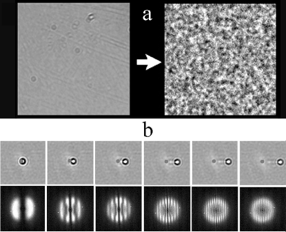
With DDM, one can in fact obtain fast measurements of the intensity correlation function at very low angles. Recalling that there is a one-to-one correspondence between the spatial frequencies of the image and the scattering wave-vectors, and using the Parseval’s theorem, which states that the integral of the square of a function is equal to the integral of the square of its Fourier transform,Goodman (2005) the total variance can indeed be written also as

$$\sigma^{2}(t)=\int|\widetilde{\Delta I}(f_{x},f_{y};t)|^{2}\mathrm{d}f_{x}\mathrm{d}f_{y},$$

where $\widetilde{\Delta I}(f_{x},f_{y};t)=\mathscr{F}[\Delta I(x,y;t)]$. Hence, by Fourier-transforming the image differences, one can extract the Brownian dynamics of the particles.Cerbino (2007)

V.3 Ghost Particle Velocimetry (GPV)

Particle Imaging Velocimetry is extensively used to monitor fluid flow in microfluidics systems, which are becoming widespread in academic and company research labs. Individual tracking, however, requires particles large enough to be optically resolved, which therefore perturb the flow over spatial scales that, in microfluidics, may be comparable to those of the investigated structures. This limitation can be overcome by resorting to more sophisticated methods such as micro-scale Particle Imaging Velocimetry ($\mu$PIV), which exploits small fluorescent tracers that do not need to be individually resolved. In this alternative approach, the fluid average velocity within a small region is rather found by detecting fluorescence intensity fluctuations and evaluating the spatial cross-correlation of two images taken at different times with a suitable frame rate.Lindken et al. (2009) However, $\mu$PIV instrumentation requires a rather expensive optical setup, usually including a pulsed laser source synchronized with a high resolution fast CCD camera.

As we mentioned in section III.3, NFS techniques provides a simple, efficient, and much cheeper method for tracking fluid motion that overcomes the main limitation of standard PIV, since particles that are smaller than the optical resolution limit can be used. Microfluidic applications, however, require velocimetry to be made under a microscope on microfluidic chips that have generally a poor optical quality: feeding in an additional laser source and setting the configuration required to measure near-field scattering is surely inconvenient, if not unfeasible. An alternative approach to quantitatively map fluid flow in microfluidic devices is what we call “Ghost Particle Velocimetry” (GPV), which uses the same procedures of NFS velocimetry, but within a DDM optical scheme.Buzzaccaro et al. (2013) Figure 7b, for instance, which refer to an experiment made using a standard microscope and white light, shows that two basic strategies for extracting the local fluid velocity discussed in Section III.2 can be used with no relevant change in a DDM configuration.

At variance with a standard NFS experiment, however, the depth of the region probed in GPV is extremely limited, because of the very small size of coherence area of the illumination source: in fact, it is much smaller than the depth of focus of the objective, so that mapping of the velocity field can be done by focusing the objective on the object plane itself. In a microfluidic geometry, this allows to simultaneously obtain, for instance, a detailed image of the channel. GPV also allows for an appreciable resolution along the optical axis, yielding 2D sections of the flow pattern separated by a few tens of micrometers. What is really interesting, however, is that the size of the particles used as tracers does not matter, as long as they scatters sufficiently strong (remember indeed that, even for scatterers with a size $a\ll\lambda$, the near–field speckle size cannot be smaller than about $\lambda$, whereas their size on the image plane is just fixed by the NA of the objective). In fact, using GPV one can perform a detailed analysis of hydrodynamic flow using as tracers nanometric “ghost” particles that are far smaller than the microscope resolution limit.Buzzaccaro et al. (2013)

PCI, DDM, and GPV are just some examples of how a careful application of statistical optics concepts can help in devising novel powerful optical methods that bring together scattering and imaging. In fact, these techniques, and DDM in particular, are deeply related to other methods that fully exploit coherence effects, such as Digital Holography and Optical Tomography. It is therefore highly probable that in the next future these new fascinating approaches will gain more importance in the investigation of colloidal systems.