Curve shortening-straightening flow for
non-closed planar curves with infinite length

Abstract

We consider a motion of non-closed planar curves with infinite length. The motion is governed by a steepest descent flow for the geometric functional which consists of the sum of the length functional and the total squared curvature. We call the flow shortening-straightening flow. In this paper, first we prove a long time existence result for the shortening-straightening flow for non-closed planar curves with infinite length. Then we show that the solution converges to a stationary solution as time goes to infinity. Moreover we give a classification of the stationary solution.

1 Introduction

There are various studies about the steepest descent flow for geometric functional defined on closed curves, for example, the shortening flow ([1], [4], [5]), the straightening flow for curve with fixed total length ([7], [11], [12]), and the straightening flow for curve with fixed local length ([6], [9]). In this paper, we consider the steepest descent flow called shortening-straightening flow.

Let $\gamma$ be a planar curve, $\kappa$ be the curvature, and $s$ denote the arc-length parameter of $\gamma$. For $\gamma$, we consider the following geometric functional

(1.1) $$E(\gamma)=\lambda^{2}\mathcal{L}(\gamma)+\mathcal{E}(\gamma),$$

where

$$\mathcal{L}(\gamma)=\int_{\gamma}ds,\qquad\mathcal{E}(\gamma)=\int_{\gamma}\kappa^{2}\,ds,$$

and $\lambda$ is a given non-zero constant. The steepest descent flow for (1.1) is given by the system

(1.2) $$\partial_{t}\gamma=(-2\partial^{2}_{s}\kappa-\kappa^{3}+\lambda^{2}\kappa)\bm{\nu},$$

where $\bm{\nu}$ is the unit normal vector of the curve pointing in the direction of the curvature. The functional $\mathcal{L}(\gamma)$ denotes the length functional of $\gamma$. We call the steepest descent flow for length functional the curve shortening flow. On the other hand, the functional $\mathcal{E}$ is well known as the total squared curvature or one dimensional Willmore functional. The steepest descent flow for the functional is called the curve straightening flow. Thus we call (1.2) the shortening-straightening flow in this paper.

We mention the known results of shortening-straightening flow. In 1996, it has been proved by A. Polden ([10]) that the equation (1.2) admits smooth solutions globally defined in time, when the initial curve is closed and has finite length (i.e., compact without boundary). Furthermore, G. Dziuk, E. Kuwert, and R. Schätzle ([3]) extended the result of [10] to closed curves with finite length in $\mathbb{R}^{n}$.

We are interested in the following problem: “What is the dynamics of non-closed planar curve with infinite length governed by shortening-straightening flow?” In this paper, we prove that there exists a long time solution of shortening-straightening flow starting from smooth planar curve with infinite length. Moreover we show that the solution converges to a stationary solution as $t\to\infty$. Namely, we consider the following initial value problem:

(SS) $$\begin{cases}&\partial_{t}\gamma=(-2\partial^{2}_{s}\kappa-\kappa^{3}+\lambda^{2}\kappa)\bm{\nu},\\ &\gamma(x,0)=\gamma_{0}(x).\end{cases}$$

The initial curve $\gamma_{0}$ is a smooth non-closed planar curve with infinite length. Moreover we assume that $\gamma_{0}$ is allowed to have self-intersections but must be close to an axis in a $C^{1}$ sense as $\left|x\right|\to\infty$. More precisely, $\gamma_{0}(x)=(\phi_{0}(x),\psi_{0}(x)):\mathbb{R}\to\mathbb{R}^{2}$ satisfies the following assumptions:

(1.3) $$\left|{\gamma_{0}}^{\prime}(x)\right|\equiv 1,$$

(1.4) $$\partial^{m}_{x}\kappa_{0}\in L^{2}(\mathbb{R})\quad\text{\rm for all}\,\,\,\,m\geq 0,$$

(1.5) $$\lim_{x\to\infty}{\phi_{0}(x)}=\infty,\quad\lim_{x\to-\infty}{\phi_{0}(x)}=-\infty,\quad\lim_{\left|x\right|\to\infty}{\phi^{\prime}_{0}(x)}=1,$$

(1.6) $$\psi_{0}(x)=O(x^{-\alpha})\,\,\,\text{for \,some}\,\,\,\alpha>\frac{1}{2}\,\,\,\text{as}\,\,\,\left|x\right|\to\infty,\quad\psi^{\prime}_{0}\in L^{2}(\mathbb{R}),$$

We state the main result of this paper in a concise form:

Theorem 1.1.

Let $\gamma_{0}(x)$ be a planar curve satisfying (1.3)–(1.6). Then there exist a family of smooth planar curves $\gamma(x,t):\mathbb{R}\times[0,\infty)\to\mathbb{R}^{2}$ satisfying (SS). Moreover, there exist sequences $\{t_{j}\}^{\infty}_{j=1}$ and $\{p_{j}\}^{\infty}_{j=1}$ and a smooth curve $\hat{\gamma}:\mathbb{R}\to\mathbb{R}^{2}$ such that $\gamma(\cdot,t_{j})-p_{j}$ converges to $\hat{\gamma}(\cdot)$ as $t_{j}\to\infty$ up to a reparametrization. The curve $\hat{\gamma}$ satisfies $\mathcal{E}(\hat{\gamma})<\infty$ and the curvature $\hat{\kappa}$ is a solution of

$$2\partial^{2}_{s}\hat{\kappa}+\hat{\kappa}^{3}-\lambda^{2}\hat{\kappa}=0.$$

Generally, in order to prove a long time existence of a steepest descent flow for a functional, we have to make use of a priori boundedness which proceeds from the functional. Thus the functional must be bounded at least for an initial state. However our functional $E$ is unbounded, because we consider planar curves with infinite length. This is a difficulty of our problem. One of the contribution of Theorem 1.1 is to prove a long time existence of the steepest descent flow for the unbounded functional $E$. In order to overcome the difficulty we mentioned above, we construct the solution of (SS) by making use of Arzelà-Ascoli’s theorem. To define a sequence approximating a solution of (SS), we need to solve a certain compact case with fixed boundary.

Concerning the classification of stationary state, one of the types is a straight line. This is corresponding to a trivial stationary state. On the other hand, the other one corresponds to a non-trivial stationary state. We give not only a classification but also a characterization of them (see Theorem 3.7). Although a dynamical aspect of solution of (SS) is an open problem, to classify and to characterize the stationary state is an important step to comprehend the dynamics.

The paper is organized as follows: In Section 2, we prove that, for a non-closed planar curve with finite length, there exists a unique long time classical solution of (1.2) with certain boundary conditions. Furthermore we show that the solution converges to a stationary solution along a sequence of time $\{t_{j}\}_{j}$ with $t_{j}\to\infty$. In Section 3, we prove (i) a long time existence of solution of (SS) and a certain asymptotic profile of the solution as $\left|x\right|\to\infty$ (Theorem 3.6), (ii) a subconvergence of the solution to a stationary solution, (iii) a classification of the stationary solutions (Theorem 3.7), and (iv) a characterization of a dynamical aspect of the solution of (SS) (Theorem 3.8).

2 Compact case with fixed boundary

Let $\Gamma_{0}(x):[0,L]\to\mathbb{R}^{2}$ be a smooth planar curve and $k_{0}(x)$ denote the curvature. Let $\Gamma_{0}(x)$ satisfy

(2.1) $$\left|{\Gamma_{0}}^{\prime}(x)\right|\equiv 1,\quad\Gamma_{0}(0)=(0,0),\quad\Gamma_{0}(L)=(R,0),\quad k_{0}(0)=k_{0}(L)=0,$$

where $L>0$ and $R>0$ are given constants. We consider the following initial boundary value problem:

(CSS) $$\begin{cases}&\partial_{t}\gamma=(-2\partial^{2}_{s}\kappa-\kappa^{3}+\lambda^{2}\kappa)\bm{\nu},\\ &\gamma(0,t)=(0,0),\quad\gamma(L,t)=(R,0),\quad\kappa(0,t)=\kappa(L,t)=0,\\ &\gamma(x,0)=\Gamma_{0}(x)\end{cases}$$

The purpose of this section is to prove the following theorem:

Theorem 2.2.

Let $\Gamma_{0}$ be a smooth planar curve satisfying the condition (2.1). Then there exists a unique classical solution of (CSS) for any time $t>0$.

2.1 Short time existence

First we show a short time existence of solution to (CSS). Let

(2.2) $$\gamma(x,t)=\Gamma_{0}(x)+d(x,t)\bm{\nu}_{0}(x),$$

where $d(x,t):[0,L]\times[0,\infty)\to\mathbb{R}$ is an unknown scalar function and $\bm{\nu}_{0}(x)$ is the unit normal vector of $\Gamma_{0}(x)$, i.e., $\bm{\nu}_{0}(x)=\mathfrak{R}{\Gamma_{0}}^{\prime}(x)=\bigl{(}\begin{smallmatrix}0&-1\\ 1&0\end{smallmatrix}\bigr{)}{\Gamma_{0}}^{\prime}(x)$. Under the formulation (2.2), the boundary conditions $\gamma(0,t)=(0,0)$ and $\gamma(L,t)=(R,0)$ are reduced to

(2.3) $$d(0,t)=d(L,t)=0.$$

With the aid of Frenet-Serret’s formula ${\Gamma_{0}}^{\prime\prime}=k_{0}\bm{\nu}_{0}$ and ${\bm{\nu}_{0}}^{\prime}=-k_{0}{\Gamma_{0}}^{\prime}$, we have

$$\partial_{x}\gamma =(1-k_{0}d){\Gamma_{0}}^{\prime}+\partial_{x}d\bm{\nu}_{0},$$

$$\mathfrak{R}\partial_{x}\gamma =-\partial_{x}d{\Gamma_{0}}^{\prime}+(1-k_{0}d)\bm{\nu}_{0},$$

$$\partial^{2}_{x}\gamma =(-{k_{0}}^{\prime}d-2k_{0}\partial_{x}d){\Gamma_{0}}^{\prime}+(\partial^{2}_{x}d+k_{0}-{k_{0}}^{2}d)\bm{\nu}_{0},$$

$$\kappa =\dfrac{\partial^{2}_{x}\gamma\cdot\mathfrak{R}\partial_{x}\gamma}{\left|\partial_{x}\gamma\right|^{3}}=\dfrac{\partial_{x}d({k_{0}}^{\prime}d+2k_{0}\partial_{x}d)+(1-k_{0}d)(\partial^{2}_{x}d+k_{0}-{k_{0}}^{2}d)}{\left\{(1-k_{0}d)^{2}+(\partial_{x}d)^{2}\right\}^{3/2}}.$$

Thus the condition $\kappa(0,t)=\kappa(L,t)=0$ implies

(2.4) $$\partial^{2}_{x}d(0,t)=\partial^{2}_{x}d(L,t)=0.$$

Let $s=s(x,t)$ denote the arc length parameter of $\gamma(x,t)$. Since

$$s(x,t)=\int^{x}_{0}\left|\partial_{x}\gamma(x,t)\right|\,dx=\int^{x}_{0}\left\{(1-k_{0}(x)d(x,t))^{2}+(\partial_{x}d(x,t))^{2}\right\}^{1/2}\,dx,$$

we have

(2.5) $$\dfrac{\partial s}{\partial x}:=\left|\gamma_{d}\right|=\left\{(1-k_{0}(x)d(x,t))^{2}+(\partial_{x}d(x,t))^{2}\right\}^{1/2}.$$

Combining the relation (2.5) with

$$\dfrac{\partial}{\partial s}=\dfrac{\partial/\partial x}{\partial s/\partial x},$$

we obtain

$$\dfrac{\partial}{\partial s}=\dfrac{\partial_{x}}{\left|\gamma_{d}\right|}.$$

Then we see that

$$\partial^{2}_{s}\kappa=\dfrac{\partial_{x}}{\left|\gamma_{d}\right|}\left(\dfrac{\partial_{x}}{\left|\gamma_{d}\right|}\left(\dfrac{\partial_{x}d(\partial_{x}k_{0}d+2k_{0}\partial_{x}d)+(1-k_{0}d)(\partial^{2}_{x}d+k_{0}-{k_{0}}^{2}d)}{\left|\gamma_{d}\right|^{3}}\right)\right).$$

This is reduced to

$$\partial^{2}_{s}\kappa=\dfrac{1}{\left|\gamma_{d}\right|^{5}}\partial^{2}_{x}\alpha_{3}-\dfrac{7}{\left|\gamma_{d}\right|^{6}}\partial_{x}\left|\gamma_{d}\right|\partial_{x}\alpha_{3}+\left\{-\dfrac{3}{\left|\gamma_{d}\right|^{6}}\partial^{2}_{x}\left|\gamma_{d}\right|+\dfrac{15}{\left|\gamma_{d}\right|^{7}}\left(\partial_{x}\left|\gamma_{d}\right|\right)^{2}\right\}\alpha_{3},$$

where

$$\alpha_{3}=\partial_{x}d(\partial_{x}k_{0}d+2k_{0}\partial_{x}d)+(1-k_{0}d)(\partial^{2}_{x}d+k_{0}-{k_{0}}^{2}d).$$

Setting

$$\alpha_{1} =\partial_{x}k_{0}d+k_{0}\partial_{x}d,$$

$$\alpha_{2} =\partial_{x}d\partial^{2}_{x}d+\alpha_{1}(k_{0}d-1),$$

$$\alpha_{4} =\partial_{x}d\partial^{3}_{x}d+(\partial^{2}_{x}d)^{2}+{\alpha_{1}}^{2}+\partial_{x}\alpha_{1}(k_{0}d-1),$$

we have

$$\partial_{x}\left|\gamma_{d}\right|=\dfrac{\alpha_{2}}{\left|\gamma_{d}\right|},\qquad\partial^{2}_{x}\left|\gamma_{d}\right|=-\dfrac{{\alpha_{2}}^{2}}{\left|\gamma_{d}\right|^{3}}+\dfrac{\alpha_{4}}{\left|\gamma_{d}\right|}.$$

Thus $\partial^{2}_{s}\kappa$ is written as

$$\partial^{2}_{s}\kappa=\dfrac{1}{\left|\gamma_{d}\right|^{5}}\partial^{2}_{x}\alpha_{3}-\dfrac{1}{\left|\gamma_{d}\right|^{7}}\left(7\alpha_{2}\partial_{x}\alpha_{3}+3\alpha_{3}\alpha_{4}\right)+\dfrac{18}{\left|\gamma_{d}\right|^{9}}{\alpha_{2}}^{2}\alpha_{3}.$$

Since $\kappa=\alpha_{3}/\left|\gamma_{d}\right|^{3}$ and

$$\partial_{t}\gamma=\partial_{t}d\bm{\nu}_{0},$$

we have

$$\partial_{t}d =\left\{-\dfrac{2}{\left|\gamma_{d}\right|^{4}}\partial^{2}_{x}\alpha_{3}+\dfrac{14}{\left|\gamma_{d}\right|^{6}}\alpha_{2}\partial_{x}\alpha_{3}+\dfrac{6}{\left|\gamma_{d}\right|^{6}}\alpha_{3}\alpha_{4}-\dfrac{36}{\left|\gamma_{d}\right|^{8}}{\alpha_{2}}^{2}\alpha_{3}-\dfrac{{\alpha_{3}}^{3}}{\left|\gamma_{d}\right|^{8}}+\dfrac{\lambda^{2}\alpha_{3}}{\left|\gamma_{d}\right|^{2}}\right\}\dfrac{1}{1-k_{0}d}$$

$$=-\dfrac{2}{\left|\gamma_{d}\right|^{4}}\partial^{4}_{x}d+\Phi(d).$$

Setting $A(d)=(-2/\left|\gamma_{d}\right|^{4})\partial^{4}_{x}$, the problem (CSS) is written in terms of $d$ as follows:

(2.6) $$\begin{cases}&\partial_{t}d=A(d)d+\Phi(d),\\ &d(0,t)=d(L,t)=d^{\prime\prime}(0,t)=d^{\prime\prime}(L,t)=0,\\ &d(x,0)=d_{0}(x)=0.\end{cases}$$

We find a smooth solution of (2.6) for a short time. To do so, we need to show the operator $A_{0}:=A(d_{0})$ is a sectorial operator. Since $A_{0}=-2\partial^{4}_{x}$, first we consider the boundary value problem

(2.7) $$\begin{cases}&\partial^{4}_{x}\varphi+\mu\varphi=f,\\ &\varphi(0)=\varphi(L)=\varphi^{\prime\prime}(0)=\varphi^{\prime\prime}(L)=0,\end{cases}$$

where $\mu$ is a constant. The solution of (2.7) is written as

(2.8) $$\varphi(x)=\int^{L}_{0}G(x,\xi)f(\xi)\,d\xi,$$

where $G(x,\xi)$ is a Green function given by

(2.9) $$G(x,\xi)=\begin{cases}\vspace{0.2cm}\dfrac{1}{(2\mu_{*})^{3}}(g_{1}(\xi)g_{2}(x)+g_{3}(\xi)g_{4}(x))\quad&\text{for}\quad 0\leq x\leq\xi,\\ \dfrac{1}{(2\mu_{*})^{3}}(g_{1}(x)g_{2}(\xi)+g_{3}(x)g_{4}(\xi))\quad&\text{for}\quad\xi<x\leq L.\\ \end{cases}$$

Here the functions $g_{1}$, $g_{2}$, $g_{3}$, $g_{4}$, and constants $K_{0}$, $K_{1}$, $K_{2}$, $\mu_{*}$ are given by

$$g_{1}(\zeta) =\cos{\mu_{*}\zeta}\sinh{\mu_{*}\zeta}-\sin{\mu_{*}\zeta}\cosh{\mu_{*}\zeta},$$

$$g_{2}(\zeta) =e^{\mu_{*}\zeta}\cos{\mu_{*}\zeta}-\dfrac{K_{1}}{K_{0}}\cos{\mu_{*}\zeta}\sinh{\mu_{*}\zeta}+\dfrac{K_{2}}{K_{0}}\sin{\mu_{*}\zeta}\cosh{\mu_{*}\zeta},$$

$$g_{3}(\zeta) =\cos{\mu_{*}\zeta}\sinh{\mu_{*}\zeta}+\sin{\mu_{*}\zeta}\cosh{\mu_{*}\zeta},$$

$$g_{4}(\zeta) =-e^{\mu_{*}\zeta}\sin{\mu_{*}\zeta}+\dfrac{K_{1}}{K_{0}}\sin{\mu_{*}\zeta}\cosh{\mu_{*}\zeta}+\dfrac{K_{2}}{K_{0}}\cos{\mu_{*}\zeta}\sinh{\mu_{*}\zeta},$$

$$K_{0} =2\cos^{2}{\mu_{*}L}\sinh^{2}{\mu_{*}L}+2\sin^{2}{\mu_{*}L}\cosh^{2}{\mu_{*}L},$$

$$K_{1} =\dfrac{e^{2\mu_{*}L}-\cos{2\mu_{*}L}}{2},\quad K_{2}=-\dfrac{\sin{2\mu_{*}L}}{2},\quad\mu_{*}=\dfrac{\mu^{1/4}}{\sqrt{2}}.$$

By virtue of (2.8) and (2.9), we see that the solution of (2.7) satisfies a priori estimate

(2.10) $$\left\|\varphi\right\|_{W^{4}_{p}(0,L)}\leq C\left\|f\right\|_{L^{p}(0,L)}$$

for any $p\geq 1$. Using the a priori estimate (2.10), we show that the operator $A_{0}$ generates an analytic semigroup on $L^{p}(0,L)$. Moreover we can verify that $A_{0}:h^{4+4\theta}_{B}([0,L])\to h^{4\theta}_{B}([0,L])$ is an infinitesimal generator of an analytic semigroup on $h^{4\theta}_{B}([0,L])$, where $0<\theta<1/4$ (for example, see [8]). Here $h^{\alpha}_{B}([0,L])$ is a little Hölder space with boundary condition:

(2.11) $$h^{\alpha}_{B}([0,L])=\begin{cases}\left\{u\in h^{\alpha}([0,L])\mid u(0)=u(L)=u^{\prime\prime}(0)=u^{\prime\prime}(L)=0\right\}\quad\text{if}\quad\alpha>2,\\ \left\{u\in h^{\alpha}([0,L])\mid u(0)=u(L)=0\right\}\quad\text{if}\quad 0<\alpha<2.\end{cases}$$

Since the equation in (2.6) is a fourth order quasilinear parabolic equation, we shall prove a short time existence of (2.6) as follows. Letting $B(d):=A(d)-A_{0}$, the system (2.6) is written as

(2.12) $$\begin{cases}&\partial_{t}d=A_{0}d+B(d)d+\Phi(d),\\ &d(0,t)=d(L,t)=d^{\prime\prime}(0,t)=d^{\prime\prime}(L,t)=0,\\ &d(x,0)=d_{0}(x)=0.\end{cases}$$

And then, we find a solution of (2.12) for a short time by using contraction mapping principle. Indeed, making use of the maximal regularity property and continuous interpolation spaces, we see that there exists a unique classical solution of (2.12), i.e., (2.6), in the class $C([0,T];h^{4+4\theta}_{B}([0,L]))\cap C^{1}([0,T];h^{4\theta}_{B}([0,L]))$, where $T>0$ is sufficiently small. And then we obtain the regularity by a standard bootstrap argument (see [8]). Then we obtain the following:

Lemma 2.1.

Let $\Gamma_{0}$ be a smooth curve satisfying (2.1). Then there exists a constant $T>0$ such that the problem (2.6) has a unique smooth solution for $0\leq t<T$.

Lemma 2.1 implies the existence of unique solution of (CSS) for a short time:

Theorem 2.3.

Let $\Gamma_{0}(x)$ be a smooth curve satisfying (2.1). Then there exist a constant $T>0$ and a smooth curve $\gamma(x,t)$ such that $\gamma(x,t)$ is a unique classical solution of the problem (CSS) for $0\leq t<T$.

2.2 Long time existence

Next we shall prove a long time existence of solution to (CSS). Let us set

$$F^{\lambda}=2\partial^{2}_{s}\kappa+\kappa^{3}-\lambda^{2}\kappa.$$

Then the gradient flow (1.2) is written as

$$\partial_{t}\gamma=-F^{\lambda}\bm{\nu}.$$

Lemma 2.2.

Under (1.2), the following commutation rule holds:

$$\partial_{t}\partial_{s}=\partial_{s}\partial_{t}-\kappa F^{\lambda}\partial_{s}.$$

Lemma 2.2 gives us the following:

Lemma 2.3.

Let $\gamma(x,t)$ satisfy (1.2). Then the curvature $\kappa(x,t)$ of $\gamma(x,t)$ satisfies

(2.13) $$\partial_{t}\kappa =-\partial^{2}_{s}F^{\lambda}-\kappa^{2}F^{\lambda}$$

$$=-2\partial^{4}_{s}\kappa-5\kappa^{2}\partial^{2}_{s}\kappa+\lambda^{2}\partial^{2}_{s}\kappa-6\kappa(\partial_{s}\kappa)^{2}-\kappa^{5}+\lambda^{2}\kappa^{3}.$$

Furthermore, the line element $ds$ of $\gamma(x,t)$ satisfies

(2.14) $$\partial_{t}ds=\kappa F^{\lambda}ds=(2\kappa\partial^{2}_{s}\kappa+\kappa^{4}-\lambda^{2}\kappa^{2})ds.$$

Here we introduce the following notation for a convenience.

Definition 2.1.

([2]) We use the symbol $\mathfrak{q}^{r}(\partial^{l}_{s}\kappa)$ for a polynomial with constant coefficients such that each of its monomials is of the form

$$\prod^{N}_{i=1}\partial^{j_{i}}_{s}\kappa\quad\text{\rm with}\quad 0\leq j_{i}\leq l\quad\text{\rm and}\quad N\geq 1$$

with

$$r=\sum^{N}_{i=1}(j_{i}+1).$$

By virtue of Lemmas 2.2 and 2.3, we have

Lemma 2.4.

For any $j\in\mathbb{N}$, the following formula holds:

(2.15) $$\partial_{t}\partial^{j}_{s}\kappa=-2\partial^{j+4}_{s}\kappa-5\kappa^{2}\partial^{j+2}_{s}\kappa+\lambda^{2}\partial^{j+2}_{s}\kappa+\lambda^{2}\mathfrak{q}^{j+3}(\partial^{j}_{s}\kappa)+\mathfrak{q}^{j+5}(\partial^{j+1}_{s}\kappa).$$

Proof.

The case $j=0$ in (2.15) has been already proved in Lemma 2.3, where $\mathfrak{q}^{5}(\partial_{s}\kappa)=-6\kappa(\partial_{s}\kappa)^{2}-\kappa^{5}$ and $\mathfrak{q}^{3}(\kappa)=\kappa^{3}$. Next suppose that the formula (2.15) holds for $j-1$. Then we have

$$\partial_{t}\partial^{j}_{s}\kappa =\partial_{s}\partial_{t}\partial^{j-1}_{s}\kappa-\kappa F^{\lambda}\partial^{j}_{s}\kappa$$

$$=\partial_{s}\left\{-2\partial^{j+3}_{s}\kappa-5\kappa^{2}\partial^{j+1}_{s}\kappa+\lambda^{2}\partial^{j+1}_{s}\kappa+\lambda^{2}\mathfrak{q}^{j+2}(\partial^{j-1}_{s}\kappa)+\mathfrak{q}^{j+4}(\partial^{j}_{s}\kappa)\right\}$$

$$\qquad-\kappa(2\partial^{2}_{s}\kappa+\kappa^{3}-\lambda\kappa^{2})\partial^{j}_{s}\kappa$$

$$=-2\partial^{j+4}_{s}\kappa-5\kappa^{2}\partial^{j+2}_{s}\kappa+\lambda^{2}\partial^{j+2}_{s}\kappa+\lambda^{2}\mathfrak{q}^{j+3}(\partial^{j}_{s}\kappa)+\mathfrak{q}^{j+5}(\partial^{j+1}_{s}\kappa).$$

∎

From the boundary condition of (CSS), we see that the curvature $\kappa$ satisfies the following:

Lemma 2.5.

Let $\kappa(x,t)$ be the curvature of $\gamma(x,t)$ satisfying (CSS). Then, for any $m\in\mathbb{N}$, it holds that

(2.16) $$\partial^{2m}_{s}\kappa(0,t)=\partial^{2m}_{s}\kappa(L,t)=0.$$

Proof.

First we show the case where $m=1$, $2$. Differentiating the boundary condition $\gamma(0,t)=(0,0)$ and $\gamma(L,t)=(R,0)$ with respect to $t$, we have $\partial_{t}\gamma(0,t)=\partial_{t}\gamma(L,t)=0$. From $\kappa(0,t)=\kappa(L,t)=0$ and the equation (1.2), we see that $\partial^{2}_{s}\kappa(0,t)=\partial^{2}_{s}\kappa(L,t)=0$. Since $\partial_{t}\kappa(0,t)=\partial_{t}\kappa(L,t)=0$, the equation (2.13) yields $\partial^{4}_{s}\kappa(0,t)=\partial^{4}_{s}\kappa(L,t)=0$.

Next, suppose that $\partial^{2n}_{s}\kappa(0,t)=\partial^{2n}_{s}\kappa(L,t)=0$ holds for any natural numbers $0\leq n\leq m$. Lemma 2.4 gives us

$$\partial_{t}\partial^{2m-2}_{s}\kappa =-2\partial^{2m+2}_{s}\kappa-5\kappa^{2}\partial^{2m}_{s}\kappa+\lambda^{2}\partial^{2m}_{s}\kappa+\lambda^{2}\mathfrak{q}^{2m+1}(\partial^{2m-2}_{s}\kappa)+\mathfrak{q}^{2m+3}(\partial^{2m-1}_{s}\kappa).$$

Since any monomials of $\mathfrak{q}^{2m+1}(\partial^{2m-2}_{s}\kappa)$ and $\mathfrak{q}^{2m+3}(\partial^{2m-1}_{s}\kappa)$ contain at least one of the terms $\partial^{2l}_{s}\kappa$ $(l=0$, $1$, $2$, $\cdots$, $m-1)$, we obtain $\partial^{2m+2}_{s}\kappa(0,t)=\partial^{2m+2}_{s}\kappa(L,t)=0$. ∎

Let us define $L^{p}$ norm with respect to the arc length parameter of $\gamma$. For a function $f(s)$ defined on $\gamma$, we write

$$\left\|f\right\|_{L^{p}_{s}} =\left\{\int_{\gamma}\left|f(s)\right|^{p}\,ds\right\}^{\frac{1}{p}},$$

$$\left\|f\right\|_{L^{\infty}_{s}} =\sup_{s\in[0,\mathcal{L}(\gamma)]}{\left|f(s)\right|},$$

where $\mathcal{L}(\gamma)$ denotes the length of $\gamma$.

In the following, we make use of the following interpolation inequalities:

Lemma 2.6.

Let $\gamma(x,t)$ be a solution of (CSS). Let $u(x,t)$ be a function defined on $\gamma$ and satisfy

$$\partial^{2m}_{s}u(0,t)=\partial^{2m}_{s}u(L,t)=0$$

for any $m\in\mathbb{N}$. Then, for integers $0\leq p<q<r$, it holds that

(2.17) $$\left\|\partial^{q}_{s}u\right\|_{L^{2}_{s}}\leq\left\|\partial^{p}_{s}u\right\|_{L^{2}_{s}}^{\frac{r-q}{r-p}}\left\|\partial^{r}_{s}u\right\|_{L^{2}_{s}}^{\frac{q-p}{r-p}}.$$

Moreover, for integers $0\leq p\leq q<r$, it holds that

(2.18) $$\left\|\partial^{q}_{s}u\right\|_{L^{\infty}_{s}}\leq\sqrt{2}\left\|\partial^{p}_{s}u\right\|_{L^{2}_{s}}^{\frac{2(r-q)-1}{2(r-p)}}\left\|\partial^{r}_{s}u\right\|_{L^{2}_{s}}^{\frac{2(q-p)+1}{2(r-p)}}.$$

Proof.

Making use of Lemma 2.5, for any positive integer $n$, we have

$$\left\|\partial^{n}_{s}u\right\|_{L^{2}_{s}}^{2}=\int_{\gamma}(\partial^{n}_{s}u)^{2}\,ds=-\int_{\gamma}\partial^{n-1}_{s}u\cdot\partial^{n+1}_{s}u\,ds\leq\left\|\partial^{n-1}_{s}u\right\|_{L^{2}_{s}}\left\|\partial^{n+1}_{s}u\right\|_{L^{2}_{s}}.$$

This implies that $\log{\left\|\partial^{n}_{s}u\right\|_{L^{2}_{s}}}$ is convex with respect to $n>0$. Thus we obtain the inequality (2.17).

Next we turn to (2.18). By Lemma 2.5, we see that $\partial^{2m}_{s}u(0)=\partial^{2m}_{s}u(L)=0$ for any $m\in\mathbb{N}$. Thus the intermediate theorem implies that there exists at least one point $0<\xi<L$ such that $\partial^{2m+1}_{s}u(\xi)=0$ for each $m\in\mathbb{N}$. Hence, for each non-negative integer $n$, there exists a point $0<\xi<L$ such that $\partial^{n}_{s}u(\xi)=0$. Then we have

$$\left(\partial^{n}_{s}u(s)\right)^{2}=\int^{s}_{\xi}\left\{\left(\partial^{n}_{s}u(\tau)\right)^{2}\right\}^{\prime}\,d\tau\leq 2\left\|\partial^{n}_{s}u\right\|_{L^{2}_{s}}\left\|\partial^{n+1}_{s}u\right\|_{L^{2}_{s}}.$$

Hence we get

(2.19) $$\left\|\partial^{n}_{s}u\right\|_{L^{\infty}_{s}}\leq\sqrt{2}\left\|\partial^{n}_{s}u\right\|_{L^{2}_{s}}^{\frac{1}{2}}\left\|\partial^{n+1}_{s}u\right\|_{L^{2}_{s}}^{\frac{1}{2}}.$$

Combining (2.17) with (2.19), we obtain (2.18). ∎

By virtue of Lemma 2.5, we are able to apply Lemma 2.6 to $\kappa(x,t)$ for any $n\in\mathbb{N}$. Making use of boundedness of the energy functional at $\gamma=\Gamma_{0}$, we derive an estimate for $\left\|\kappa\right\|_{L^{2}_{s}}$:

Lemma 2.7.

The following estimate holds:

(2.20) $$\left\|\kappa\right\|_{L^{2}_{s}}^{2}\leq\left\|k_{0}\right\|_{L^{2}(0,L)}^{2}+\lambda^{2}\left(\mathcal{L}(\Gamma_{0})-R\right).$$

Proof.

Since the equation in (CSS) is the steepest descent flow for $E(\gamma)=\left\|\kappa\right\|_{L^{2}_{s}}^{2}+\lambda^{2}\mathcal{L}(\gamma)$, we have

$$\left\|\kappa\right\|_{L^{2}_{s}}^{2}+\lambda^{2}\mathcal{L}(\gamma)\leq\left\|k_{0}\right\|_{L^{2}(0,L)}^{2}+\lambda^{2}\mathcal{L}(\Gamma_{0}).$$

Clearly it holds that $\mathcal{L}(\gamma)\geq R$. Therefore we obtain (2.20). ∎

In order to use the energy method, we prepare the following:

Lemma 2.8.

For any $j\in\mathbb{N}$, it holds that

(2.21) $$\dfrac{d}{dt}\left\|\partial^{j}_{s}\kappa\right\|_{L^{2}_{s}}^{2} =-2\left\|\partial^{j+2}_{s}\kappa\right\|_{L^{2}_{s}}^{2}-2\lambda^{2}\left\|\partial^{j+1}_{s}\kappa\right\|_{L^{2}_{s}}^{2}$$

$$\qquad+\lambda^{2}\int_{\gamma}\mathfrak{q}^{2j+4}(\partial^{j}_{s}\kappa)\,ds+\int_{\gamma}\mathfrak{q}^{2j+6}(\partial^{j+1}_{s}\kappa).$$

Proof.

By virtue of Lemma 2.4, we have

$$\dfrac{d}{dt}\left\|\partial^{j}_{s}\kappa\right\|_{L^{2}_{s}}^{2} =\int_{\gamma}2\partial^{j}_{s}\kappa\partial_{t}\partial^{j}_{s}\kappa\,ds+\int_{\gamma}(\partial^{j}_{s}\kappa)^{2}\kappa F^{\lambda}\,ds$$

$$=\int_{\gamma}2\partial^{j}_{s}\kappa\left\{-2\partial^{j+4}_{s}\kappa-5\kappa^{2}\partial^{j+2}_{s}\kappa+\lambda^{2}\partial^{j+2}_{s}\kappa+\lambda^{2}\mathfrak{q}^{j+3}(\partial^{j}_{s}\kappa)+\mathfrak{q}^{j+5}(\partial^{j+1}_{s}\kappa)\right\}\,ds$$

$$\qquad+\int_{\gamma}\kappa\partial^{j}_{s}\kappa(2\partial^{2}_{s}\kappa+\kappa^{3}-\lambda\kappa^{2})\,ds.$$

By integrating by parts, we get

$$\int_{\gamma}\kappa^{2}\partial^{j}_{s}\kappa\partial^{j+2}_{s}\kappa\,ds=-\int_{\gamma}\left\{2\kappa\partial_{s}\kappa\partial^{j}_{s}\kappa\partial^{j+1}_{s}\kappa+\kappa^{2}(\partial^{j+1}_{s}\kappa)^{2}\right\}\,ds.$$

Consequently we obtain (2.21). ∎

Using Lemmas 2.7 and 2.8, we derive the estimate for the derivative of $\|\partial^{j}_{s}\kappa\|_{L^{2}_{s}}^{2}$ with respect to $t$.

Lemma 2.9.

For any $j\in\mathbb{N}$, we have

$$\dfrac{d}{dt}\left\|\partial^{j}_{s}\kappa\right\|_{L^{2}_{s}}^{2}\leq C\left\|\kappa\right\|_{L^{2}_{s}}^{4j+6}+C\left\|\kappa\right\|_{L^{2}_{s}}^{4j+10}.$$

Proof.

By Lemma 2.8, we shall estimate the right hand side of (2.21). First we focus on the term $\int_{\gamma}\mathfrak{q}^{2j+4}(\partial^{j}_{s}\kappa)\,ds$. By Definition 2.1, we have

$$\mathfrak{q}^{2j+4}(\partial^{j}_{s}\kappa)=\sum_{m}\prod^{N_{m}}_{l=1}\partial^{c_{ml}}_{s}\kappa$$

with all the $c_{ml}$ less than or equal to $j$ and

$$\sum^{N_{m}}_{l=1}(c_{ml}+1)=2j+4$$

for every $m$. Hence we have

$$\left|\mathfrak{q}^{2j+4}(\partial^{j}_{s}\kappa)\right|\leq\sum_{m}\prod^{N_{m}}_{l=1}\left|\partial^{c_{ml}}_{s}\kappa\right|.$$

Setting

$$Q_{m}=\prod^{N_{m}}_{l=1}\left|\partial^{c_{ml}}_{s}\kappa\right|,$$

it holds that

$$\int_{\gamma}\left|\mathfrak{q}^{2j+4}(\partial^{j}_{s}\kappa)\right|\,ds\leq\sum_{m}\int_{\gamma}Q_{m}\,ds.$$

We now estimate any term $Q_{m}$ by Lemma 2.6. After collecting derivatives of the same order in $Q_{m}$, we can write

(2.22) $$Q_{m}=\prod^{j}_{i=0}\left|\partial^{i}_{s}\kappa\right|^{\alpha_{mi}}\qquad\text{with}\quad\sum^{j}_{i=0}\alpha_{mi}(i+1)=2j+4.$$

Then

$$\int_{\gamma}Q_{m}\,ds=\int_{\gamma}\prod^{j}_{i=0}\left|\partial^{i}_{s}\kappa\right|^{\alpha_{mi}}\,ds\leq\prod^{j}_{i=0}\left(\int_{\gamma}\left|\partial^{i}_{s}\kappa\right|^{\alpha_{mi}}\,ds\right)^{1/\lambda_{i}}\leq\prod^{j}_{i=0}\left\|\partial^{i}_{s}\kappa\right\|_{L^{\alpha_{mi\lambda_{i}}}_{s}}^{\alpha_{mi}},$$

where the value $\lambda_{i}$ are chosen as follows: $\lambda_{i}=0$ if $\alpha_{mi}=0$ (in this case the corresponding term is not present in the product) and $\lambda_{i}=(2j+4)/(\alpha_{mi}(i+1))$ if $\alpha_{mi}\neq 0$. Clearly, $\alpha_{mi}\lambda_{i}=\frac{2j+4}{i+1}\geq\frac{2j+4}{j+1}>2$ and by the condition (2.22),

$$\sum^{j}_{i=0,\lambda_{i}\neq 0}\frac{1}{\lambda_{i}}=\sum^{j}_{i=0,\lambda_{i}\neq 0}\frac{\alpha_{mi}(i+1)}{2j+4}=1.$$

Let $k_{i}=\alpha_{mi}\lambda_{i}-2$. The fact $\alpha_{mi}\lambda_{i}>2$ implies $k_{i}>0$. Then we have

$$\left\|\partial^{i}_{s}\kappa\right\|_{L^{\alpha_{mi\lambda_{i}}}_{s}} =\left\|\partial^{i}_{s}\kappa\right\|_{L^{\infty}_{s}}^{k_{i}}\left\|\partial^{i}_{s}\kappa\right\|_{L^{2}_{s}}^{2},$$

$$\left\|\partial^{i}_{s}\kappa\right\|_{L^{\infty}_{s}}^{k_{i}} \leq 2^{\frac{k_{i}}{2}}\left\|\partial^{j+1}_{s}\kappa\right\|_{L^{2}_{s}}^{\frac{2i+1}{2j+2}k_{i}}\left\|\kappa\right\|_{L^{2}_{s}}^{\frac{2j+1-2i}{2j+2}k_{i}},$$

$$\left\|\partial^{i}_{s}\kappa\right\|_{L^{2}_{s}}^{2} \leq\left\|\partial^{j+1}_{s}\kappa\right\|_{L^{2}_{s}}^{\frac{2i}{j+1}}\left\|\kappa\right\|_{L^{2}_{s}}^{\frac{2j+2-2i}{j+1}}.$$

These imply

$$\left\|\partial^{i}_{s}\kappa\right\|_{L^{\alpha_{mi}\lambda_{i}}_{s}} \leq 2^{\frac{k_{i}}{2}}\left\|\partial^{j+1}_{s}\kappa\right\|_{L^{2}_{s}}^{\sigma_{mi}}\left\|\kappa\right\|_{L^{2}_{s}}^{1-\sigma_{mi}}$$

with

$$\sigma_{mi}=\frac{i+\frac{1}{2}-\frac{1}{\alpha_{mi}\lambda_{i}}}{j+1}.$$

Multiplying together all the estimates,

(2.23) $$\int_{\gamma}Q_{m}\,ds \leq\prod^{j}_{i=0}2^{\frac{k_{i}}{2}}\left\|\partial^{j+1}_{s}\kappa\right\|_{L^{2}_{s}}^{\alpha_{mi}\sigma_{mi}}\left\|\kappa\right\|_{L^{2}_{s}}^{\alpha_{mi}(1-\sigma_{mi})}$$

$$\leq C\left\|\partial^{j+1}_{s}\kappa\right\|_{L^{2}_{s}}^{\sum^{j}_{i=0}\alpha_{mi}\sigma_{mi}}\left\|\kappa\right\|_{L^{2}_{s}}^{\sum^{j}_{i=0}\alpha_{mi}(1-\sigma_{mi})}.$$

Then we compute

$$\sum^{j}_{i=0}\alpha_{mi}\sigma_{mi}=\sum^{j}_{i=0}\frac{\alpha_{mi}(i+\frac{1}{2})-\frac{1}{\lambda_{i}}}{j+1}=\frac{\sum^{j}_{i=0}\alpha_{mi}(i+\frac{1}{2})-1}{j+1}$$

and using again the rescaling condition in (2.22),

$$\sum^{j}_{i=0}\alpha_{mi}\sigma_{mi} =\frac{\sum^{j}_{i=0}\alpha_{mi}(i+1)-\frac{1}{2}\sum^{j}_{i=0}\alpha_{mi}-1}{j+1}$$

$$=\frac{2j+4-\frac{1}{2}\sum^{j}_{i=0}\alpha_{mi}-1}{j+1}=\frac{4j+6-\sum^{j}_{i=0}\alpha_{mi}}{2(j+1)}.$$

Since

$$\sum^{j}_{i=0}\alpha_{mi}\geq\sum^{j}_{i=0}\alpha_{mi}\frac{i+1}{j+1}=\frac{2j+4}{j+1},$$

we get

$$\sum^{j}_{i=0}\alpha_{mi}\sigma_{mi}\leq\frac{2j^{2}+4j+1}{(j+1)^{2}}=2-\frac{1}{(j+1)^{2}}<2.$$

Hence, we can apply the Young inequality to the product in the last term of inequality (2.23), in order to get the exponent $2$ on the first quantity, that is,

$$\int_{\gamma}Q_{m}\,ds\leq\frac{\delta_{m}}{2}\left\|\partial^{j+1}_{s}\kappa\right\|_{L^{2}_{s}}^{2}+C_{m}\left\|\kappa\right\|_{L^{2}_{s}}^{\beta}\leq\delta_{m}\left\|\partial^{j+1}_{s}\kappa\right\|_{L^{2}_{s}}^{2}\,ds+C_{m}\left\|\kappa\right\|_{L^{2}_{s}}^{\beta},$$

for arbitrarily small $\delta_{m}>0$ and some constant $C_{m}>0$. The exponent $\beta$ is given by

$$\beta =\sum^{j}_{i=0}\alpha_{mi}(1-\sigma_{mi})\frac{1}{1-\frac{\sum^{j}_{i=0}\alpha_{mi}\sigma_{mi}}{2}}=\frac{2\sum^{j}_{i=0}\alpha_{mi}(1-\sigma_{mi})}{2-\sum^{j}_{i=0}\alpha_{mi}\sigma_{mi}}$$

$$=\frac{2\sum^{j}_{i=0}\alpha_{mi}-\frac{4j+6-\sum^{j}_{i=0}\alpha_{mi}}{j+1}}{2-\frac{4j+6-\sum^{j}_{i=0}\alpha_{mi}}{2(j+1)}}=2\frac{2(j+1)\sum^{j}_{i=0}\alpha_{mi}-4j-6+\sum^{j}_{i=0}\alpha_{mi}}{4j+4-4j-6+\sum^{j}_{i=0}\alpha_{mi}}$$

$$=2\frac{(2j+3)\sum^{j}_{i=0}\alpha_{mi}-2(2j+3)}{\sum^{j}_{i=0}\alpha_{mi}-2}=2(2j+3).$$

Therefore we conclude

$$\int_{\gamma}Q_{m}\,ds\leq\delta_{m}\left\|\partial^{j+1}_{s}\kappa\right\|_{L^{2}_{s}}^{2}+C_{m}\left\|\kappa\right\|_{L^{2}_{s}}^{4j+6}.$$

Repeating this argument for all the $Q_{m}$ and choosing suitable $\delta_{m}$ whose sum over $m$ is less than one, we conclude that there exists a constant $C$ depending only on $j\in\mathbb{N}$ such that

$$\int_{\gamma}\mathfrak{q}^{2j+4}(\partial^{j}_{s}\kappa)\,ds\leq\left\|\partial^{j+1}_{s}\kappa\right\|_{L^{2}_{s}}^{2}+C\left\|\kappa\right\|_{L^{2}_{s}}^{4j+6}.$$

Reasoning similarly for the term $\mathfrak{q}^{2j+6}(\partial^{j+1}_{s}\kappa)$, we obtain

$$\int_{\gamma}\mathfrak{q}^{2j+6}(\partial^{j+1}_{s}\kappa)\,ds\leq\left\|\partial^{j+2}_{s}\kappa\right\|_{L^{2}_{s}}^{2}+C\left\|\kappa\right\|_{L^{2}_{s}}^{4j+10}.$$

Hence, from (2.21), we get

$$\partial_{t}\left\|\partial^{j}_{s}\kappa\right\|_{L^{2}_{s}}^{2} =-2\left\|\partial^{j+2}_{s}\kappa\right\|_{L^{2}_{s}}^{2}-2\lambda^{2}\left\|\partial^{j+1}_{s}\kappa\right\|_{L^{2}_{s}}^{2}$$

$$\qquad+\lambda^{2}\int_{\gamma}\mathfrak{q}^{2j+4}(\partial^{j}_{s}\kappa)\,ds+\int_{\gamma}\mathfrak{q}^{2j+6}(\partial^{j+1}_{s}\kappa)$$

$$\leq-\lambda^{2}\left\|\partial^{j+1}_{s}\kappa\right\|_{L^{2}_{s}}^{2}+C\left\|\kappa\right\|_{L^{2}_{s}}^{4j+6}-\left\|\partial^{j+2}_{s}\kappa\right\|_{L^{2}_{s}}^{2}+C\varepsilon\left\|\kappa\right\|_{L^{2}_{s}}^{4j+10}$$

$$\leq C\left\|\kappa\right\|_{L^{2}_{s}}^{4j+6}+C\left\|\kappa\right\|_{L^{2}_{s}}^{4j+10},$$

where $C$ depends only on $j$. ∎

Next we estimate the local length of $\gamma(x,t)$.

Lemma 2.10.

Let $\gamma(x,t)$ be a solution of (CSS) for $0\leq t<T$. Then there exist positive constants $C_{1}$ and $C_{2}$ such that the inequalities

(2.24) $$\dfrac{1}{C_{1}(\Gamma_{0},T)}\leq\left|\partial_{x}\gamma(x,t)\right|\leq C_{1}(\Gamma_{0},T),$$

(2.25) $$\left|\partial^{m}_{x}\left|\partial_{x}\gamma(x,t)\right|\right|\leq C_{2}(\Gamma_{0},T)$$

hold for any $(x,t)\in[0,L]\times[0,T]$ and integer $m\geq 1$.

Proof.

First we prove (2.24). Since

$$\partial_{x}\partial_{t}\gamma =\partial_{x}\left(-2\partial^{2}_{s}\kappa-{\kappa}^{3}+\lambda^{2}\kappa\right)\bm{\nu}+\left(-2\partial^{2}_{s}\kappa-{\kappa}^{3}+\lambda^{2}\kappa\right)\partial_{x}\bm{\nu},$$

and $\partial_{x}\bm{\nu}=\left|\partial_{x}\gamma\right|\partial_{s}\bm{\nu}=-\left|\partial_{x}\gamma\right|\kappa\partial_{s}\gamma$, we have

(2.26) $$\partial_{t}\left|\partial_{x}\gamma\right|=\dfrac{\partial_{x}\gamma\cdot\partial_{x}\partial_{t}\gamma}{\left|\partial_{x}\gamma\right|}=-\kappa\left(-2\partial^{2}_{s}\kappa-{\kappa}^{3}+\lambda^{2}\kappa\right)\left|\partial_{x}\gamma\right|.$$

Thus $\left|\partial_{x}\gamma\right|$ satisfies the initial value problem

(2.27) $$\begin{cases}\dfrac{du}{dt}=F(\kappa)u,\\ u(0)=1,\end{cases}$$

where

$$F(\kappa)=-\kappa\left(-2\partial^{2}_{s}\kappa-{\kappa}^{3}+\lambda^{2}\kappa\right).$$

Since Lemmas 2.7 and 2.9 implies that there exists a constant $C$ such that

$$\left|F(\kappa)\right|\leq C$$

for any $(x,t)\in[0,L]\times[0,T]$. Hence, for any $(x,t)\in[0,L]\times[0,T]$, we have

$$e^{-C_{1}T}\leq\left|\partial_{x}\gamma(x,t)\right|\leq e^{C_{1}T}.$$

Next we turn to the proof of (2.25). Here we have

(2.28) $$\partial^{m}_{x}F(\kappa)-\left|\partial_{x}\gamma\right|^{m}\partial^{m}_{s}F(\kappa)=P(\left|\partial_{x}\gamma\right|,\cdots,\partial^{m-1}_{x}\left|\partial_{x}\gamma\right|,F(\kappa),\cdots,\partial^{m-1}_{s}F(\kappa)).$$

Suppose that there exist constants $C_{j}(T,\Gamma_{0})$ such that

$$\sup_{(x,t)\in[0,L]\times[0,T]}\left|\partial^{j}_{x}\left|\partial_{x}\gamma\right|\right|\leq C_{j}(T,\Gamma_{0})$$

for any $0\leq j\leq m-1$. Then (2.28) implies

$$\left|\partial^{m}_{x}F(\kappa)\right|<C.$$

Differentiating the equation (2.26) with respect to $x$, we have

$$\partial_{t}\partial^{m}_{x}\left|\partial_{x}\gamma\right|=F(\kappa)\partial^{m}_{x}\left|\partial_{x}\gamma\right|+\sum^{m}_{j=1}\mbox{}_{m}C_{j}\partial^{j}_{x}F(\kappa)\partial^{m-j}_{x}\left|\partial_{x}\gamma\right|.$$

Thus $\partial^{m}_{x}\left|\partial_{x}\gamma\right|$ satisfies

(2.29) $$\begin{cases}&\partial_{t}v=F(\kappa)v+G,\\ &v(0)=0.\end{cases}$$

We can check that there exists a constant $C_{2}(T,\Gamma_{0})$ such that $\left|v\right|\leq C_{2}$. This gives us the conclusion of Lemma 2.10. ∎

Then we prove that the system (CSS) has a unique global solution in time.

Theorem 2.4.

Let $\Gamma_{0}$ be a smooth planar curve satisfying the condition (2.1). Then there exists a unique classical solution of (CSS) for any time $t>0$.

Proof.

Suppose not, then there exists a positive constant $\tilde{T}$ such that $\gamma(x,t)$ does not extend smoothly beyond $\tilde{T}$. It follows from Lemmas 2.7 and 2.9 that

$$\left\|\partial^{m}_{s}\kappa\right\|_{L^{2}_{s}}^{2}\leq\left\|\partial^{m}_{x}k_{0}\right\|_{L^{2}(0,L)}^{2}+C\tilde{T}$$

holds for any $0\leq t\leq\tilde{T}$ and $m\in\mathbb{N}$. This yields that there exists a constant $C$ such that

(2.30) $$\left\|\partial^{m}_{s}\gamma\right\|_{L^{2}_{s}}\leq C$$

for $t\in[0,\tilde{T}]$. We have already known

(2.31) $$\partial^{m}_{x}\gamma-\left|\partial_{x}\gamma\right|^{m}\partial^{m}_{s}\gamma=P(\left|\partial_{x}\gamma\right|,\cdots,\partial^{m-1}_{x}\left|\partial_{x}\gamma\right|,\gamma,\cdots,\partial^{m-1}_{s}\gamma).$$

By virtue of (2.30), (2.31), and Lemma 2.10, we see that there exists a constant $C$ such that

$$\left\|\partial^{m}_{x}\gamma\right\|_{L^{2}(0,L)}\leq C$$

for any $t\in[0,\tilde{T}]$ and $m\in\mathbb{N}$. Then $\gamma(x,t)$ extends smoothly beyond $\tilde{T}$ by Theorem 2.3. This is a contradiction. We complete the proof. ∎

2.3 Convergence to a stationary solution

Finally we shall prove that the solution $\gamma(x,t)$ converges to a stationary solution as $t\to\infty$. For this purpose, we rewrite the equation (1.2) in terms of $\gamma$ as follows:

(2.32) $$\partial_{t}\gamma=-2\partial^{4}_{s}\gamma+\left(\lambda^{2}-3\left|\partial^{2}_{s}\gamma\right|^{2}\right)\partial^{2}_{s}\gamma-3\partial_{s}\left(\left|\partial^{2}_{s}\gamma\right|^{2}\right)\partial_{s}\gamma.$$

Since the arc length parameter $s$ depends on $t$, the following rules hold:

(2.33) $$\partial_{t}\partial_{s} =\partial_{s}\partial_{t}-G^{\lambda}\partial_{s},$$

(2.34) $$\partial_{t}ds =G^{\lambda}ds,$$

where $G^{\lambda}=\partial_{s}\partial_{t}\gamma\cdot\partial_{s}\gamma$. In previous section, we prove that the initial-boundary value problem for (2.32) has a unique classical solution $\gamma(x,t)$ for any $t>0$. The solution $\gamma$ has the following property:

Lemma 2.11.

Let $\gamma(x,t)$ be the solution of (CSS). Then, for any positive integer $m$, it holds that

(2.35) $$\partial^{2m}_{s}\gamma(0,t)=\partial^{2m}_{s}\gamma(L,t)=0.$$

Proof.

First we prove that the relation

(2.36) $$\partial^{n}_{s}\gamma=\mathfrak{q}^{n-1}(\partial^{n-2}_{s}\kappa)\bm{\nu}+\mathfrak{q}^{n-1}(\partial^{n-2}_{s}\kappa)\partial_{s}\gamma$$

holds for any integers $n\geq 2$. Since $\partial^{2}_{s}\gamma=\kappa\bm{\nu}$, we see that (2.36) holds for $n=2$. Suppose that (2.36) holds for any integers $2\leq n\leq k$, where $k>2$ is some integer. Then we have

$$\partial^{k+1}_{s}\gamma =\partial^{s}\{\mathfrak{q}^{k-1}(\partial^{k-2}_{s}\kappa)\}\bm{\nu}+\mathfrak{q}^{k-1}_{s}(\partial^{k-2}_{s}\kappa)\partial_{s}\bm{\nu}+\partial^{s}\{\mathfrak{q}^{k-1}(\partial^{k-2}_{s}\kappa)\}\partial_{s}\gamma+\mathfrak{q}^{k-1}_{s}(\partial^{k-2}_{s}\kappa)\partial^{2}_{s}\gamma$$

$$=\left\{\partial^{s}\{\mathfrak{q}^{k-1}(\partial^{k-2}_{s}\kappa)\}+\kappa\mathfrak{q}^{k-1}_{s}(\partial^{k-2}_{s}\kappa)\right\}\bm{\nu}+\left\{\partial^{s}\{\mathfrak{q}^{k-1}(\partial^{k-2}_{s}\kappa)\}-\kappa\mathfrak{q}^{k-1}_{s}(\partial^{k-2}_{s}\kappa)\right\}\partial_{s}\gamma$$

$$=\mathfrak{q}^{k}(\partial^{k-1}_{s}\kappa)\bm{\nu}+\mathfrak{q}^{k}(\partial^{k-1}_{s}\kappa)\partial_{s}\gamma.$$

This implies (2.36). Then, along the same line as in the proof of Lemma 2.5, we obtain the conclusion. ∎

By virtue of Lemma 2.11, we can apply Lemma 2.6, i.e., interpolation inequalities, to $\partial^{2}_{s}\gamma$. Using the interpolation inequalities, we first prove the following estimate:

Lemma 2.12.

There exist positive constants $C_{1}$ and $C_{2}$ depending only on $\lambda$ such that

$$\left\|\partial^{4}_{s}\gamma\right\|_{L^{2}_{s}}\leq\left\|\partial_{t}\gamma\right\|_{L^{2}_{s}}+C_{1}\left\|\partial^{2}_{s}\gamma\right\|_{L^{2}_{s}}^{5}+C_{2}\left\|\partial^{2}_{s}\gamma\right\|_{L^{2}_{s}}.$$

Proof.

From (2.32), we have

$$\left\|\partial_{t}\gamma\right\|_{L^{2}_{s}}^{2} =\int_{\gamma}\left|-2\partial^{4}_{s}\gamma+\left(\lambda^{2}-3\left|\partial^{2}_{s}\gamma\right|^{2}\right)\partial^{2}_{s}\gamma-3\partial_{s}\left(\left|\partial^{2}_{s}\gamma\right|^{2}\right)\partial_{s}\gamma\right|^{2}\,ds$$

$$\geq 2\left\|\partial^{4}_{s}\gamma\right\|_{L^{2}_{s}}^{2}-2\left\|\left(\lambda^{2}-3\left|\partial^{2}_{s}\gamma\right|^{2}\right)\partial^{2}_{s}\gamma\right\|_{L^{2}_{s}}^{2}-2\left\|3\partial_{s}\left(\left|\partial^{2}_{s}\gamma\right|^{2}\right)\partial_{s}\gamma\right\|_{L^{2}_{s}}^{2}.$$

It follows from interpolation inequalities that

$$\left\|\left(\lambda^{2}-3\left|\partial^{2}_{s}\gamma\right|^{2}\right)\partial^{2}_{s}\gamma\right\|_{L^{2}_{s}}^{2} \leq 2\lambda^{4}\left\|\partial^{2}_{s}\gamma\right\|_{L^{2}_{s}}^{2}+18\left\|\left|\partial^{2}_{s}\gamma\right|^{2}\partial^{2}_{s}\gamma\right\|_{L^{2}_{s}}^{2}$$

$$\leq 2\lambda^{4}\left\|\partial^{2}_{s}\gamma\right\|_{L^{2}_{s}}^{2}+18\left\|\partial^{2}_{s}\gamma\right\|_{L^{\infty}_{s}}^{4}\left\|\partial^{2}_{s}\gamma\right\|_{L^{2}_{s}}^{2}$$

$$\leq 2\lambda^{4}\left\|\partial^{2}_{s}\gamma\right\|_{L^{2}_{s}}^{2}+72\left\|\partial^{4}_{s}\gamma\right\|_{L^{2}_{s}}\left\|\partial^{2}_{s}\gamma\right\|_{L^{2}_{s}}^{5}$$

$$\leq\varepsilon\left\|\partial^{4}_{s}\gamma\right\|_{L^{2}_{s}}^{2}+C(1/\varepsilon)\left\|\partial^{2}_{s}\gamma\right\|_{L^{2}_{s}}^{10}+2\lambda^{4}\left\|\partial^{2}_{s}\gamma\right\|_{L^{2}_{s}}^{2}.$$

Similarly we have

$$\left\|\partial_{s}\left(\left|\partial^{2}_{s}\gamma\right|^{2}\right)\partial_{s}\gamma\right\|_{L^{2}_{s}}^{2} \leq 4\left\|\partial^{2}_{s}\gamma\right\|_{L^{\infty}_{s}}^{2}\left\|\partial^{3}_{s}\gamma\right\|_{L^{2}_{s}}^{2}$$

$$\leq 4\sqrt{2}\left\|\partial^{4}_{s}\gamma\right\|_{L^{2}_{s}}^{3/2}\left\|\partial^{2}_{s}\gamma\right\|_{L^{2}_{s}}^{5/2}\leq\varepsilon\left\|\partial^{4}_{s}\gamma\right\|_{L^{2}_{s}}^{2}+C(1/\varepsilon)\left\|\partial^{2}_{s}\gamma\right\|_{L^{2}_{s}}^{10}.$$

Letting $\varepsilon=\dfrac{1}{4}$, we obtain

$$\left\|\partial^{4}_{s}\gamma\right\|_{L^{2}_{s}}^{2}\leq\left\|\partial_{t}\gamma\right\|_{L^{2}_{s}}^{2}+C_{1}\left\|\partial^{2}_{s}\gamma\right\|_{L^{2}_{s}}^{10}+C_{2}\left\|\partial^{2}_{s}\gamma\right\|_{L^{2}_{s}}^{2}.$$

∎

In order to derive the estimate of $\left\|\partial^{n}_{s}\gamma\right\|_{L^{2}_{s}}$ for $n\geq 5$, we prepare the following:

Lemma 2.13.

For any $n\in\mathbb{N}$, it holds that

$$\partial_{t}\partial^{n}_{s}\gamma=\partial^{n}_{s}\partial_{t}\gamma-\sum^{n-1}_{j=0}\partial^{j}_{s}(G^{\lambda}\partial^{n-j}_{s}\gamma).$$

Using Lemma 2.13, we prove the estimate of $\left\|\partial^{n+4}_{s}\gamma\right\|_{L^{2}_{s}}$ for any $n\in\mathbb{N}$:

Lemma 2.14.

For any $n\in\mathbb{N}$, the following estimate holds:

(2.37) $$\left\|\partial^{n+4}_{s}\gamma\right\|_{L^{2}_{s}}\leq\left\|\partial^{n}_{s}\partial_{t}\gamma\right\|_{L^{2}_{s}}+C\left\|\partial^{2}_{s}\gamma\right\|_{L^{2}_{s}}^{2n+5}+C\left\|\partial^{2}_{s}\gamma\right\|_{L^{2}_{s}}.$$

Proof.

We have already proved the case $n=0$ by Lemma 2.12. Let $n\geq 1$ fix arbitrarily. By (2.32), we have

$$\left\|\partial^{n}_{s}\partial_{t}\gamma\right\|_{L^{2}_{s}}^{2} =\left\|-2\partial^{n+4}_{s}\gamma+\partial^{n}_{s}\left\{\left(\lambda^{2}-3\left|\partial^{2}_{s}\gamma\right|^{2}\right)\partial^{2}_{s}\gamma\right\}-3\partial^{n}_{s}\left\{\partial_{s}\left(\left|\partial^{2}_{s}\gamma\right|^{2}\right)\partial_{s}\gamma\right\}\right\|_{L^{2}_{s}}^{2}$$

$$\geq 2\left\|\partial^{n+4}_{s}\gamma\right\|_{L^{2}_{s}}^{2}-2\left\|\partial^{n}_{s}\left\{\left(\lambda^{2}-3\left|\partial^{2}_{s}\gamma\right|^{2}\right)\partial^{2}_{s}\gamma\right\}\right\|_{L^{2}_{s}}^{2}-2\left\|3\partial^{n}_{s}\left\{\partial_{s}\left(\left|\partial^{2}_{s}\gamma\right|^{2}\right)\partial_{s}\gamma\right\}\right\|_{L^{2}_{s}}^{2}$$

$$:=2\left\|\partial^{n+4}_{s}\gamma\right\|_{L^{2}_{s}}^{2}-2I_{1}-2I_{2}.$$

Concerning $I_{1}$, first we have

$$\left\|\partial^{n}_{s}\partial^{2}_{s}\gamma\right\|_{L^{2}_{s}}^{2}\leq C\left\|\partial^{n+4}_{s}\gamma\right\|_{L^{2}_{s}}^{\frac{2n}{n+2}}\left\|\partial^{2}_{s}\gamma\right\|_{L^{2}_{s}}^{\frac{4}{n+2}}\leq\varepsilon\left\|\partial^{n+4}_{s}\gamma\right\|_{L^{2}_{s}}^{2}+C\left\|\partial^{2}_{s}\gamma\right\|_{L^{2}_{s}}^{2}.$$

Furthermore since

$$\partial^{n}_{s}\left(\left|\partial^{2}_{s}\gamma\right|^{2}\partial^{2}_{s}\gamma\right)=2\sum^{n}_{j=0}\mbox{}_{n}C_{j}\partial^{n-j+2}_{s}\gamma\sum^{j}_{k=0}\mbox{}_{j}C_{k}\partial^{k+2}_{s}\gamma\cdot\partial^{j-k+2}_{s}\gamma,$$

it follows from interpolation inequalities that

$$\left\|\partial^{n}_{s}\left(\left|\partial^{2}_{s}\gamma\right|^{2}\partial^{2}_{s}\gamma\right)\right\|_{L^{2}_{s}}^{2} \leq C\sum^{n}_{j=0}\sum^{j}_{k=0}\left\|\partial^{n-j+2}_{s}\gamma(\partial^{k+2}_{s}\gamma\cdot\partial^{j-k+2}_{s}\gamma)\right\|_{L^{2}_{s}}^{2}$$

$$\leq C\sum^{n}_{j=0}\sum^{j}_{k=0}\left\|\partial^{n-j+2}_{s}\gamma\right\|_{L^{2}_{s}}^{2}\left\|\partial^{k+2}_{s}\gamma\right\|_{L^{\infty}_{s}}^{2}\left\|\partial^{j-k+2}_{s}\gamma\right\|_{L^{\infty}_{s}}^{2}$$

$$\leq C\left\|\partial^{n+4}_{s}\gamma\right\|_{L^{2}_{s}}^{\frac{2n+2}{n+2}}\left\|\partial^{2}_{s}\gamma\right\|_{L^{2}_{s}}^{\frac{4n+10}{n+2}}\leq\varepsilon\left\|\partial^{n+4}_{s}\gamma\right\|_{L^{2}_{s}}^{2}+C\left\|\partial^{2}_{s}\gamma\right\|_{L^{2}_{s}}^{4n+10}.$$

Thus we have

$$I_{1}\leq(\lambda^{2}+1)\varepsilon\left\|\partial^{n+4}_{s}\gamma\right\|_{L^{2}_{s}}^{2}+C\left\|\partial^{2}_{s}\gamma\right\|_{L^{2}_{s}}^{4n+10}+C\left\|\partial^{2}_{s}\gamma\right\|_{L^{2}_{s}}^{2}.$$

Next we estimate $I_{2}$. Since

$$\partial^{n}_{s}\left\{\partial_{s}\left(\left|\partial^{2}_{s}\gamma\right|^{2}\right)\partial_{s}\gamma\right\}=2\sum^{n}_{j=0}\mbox{}_{n}C_{j}\partial^{n-j+1}_{s}\gamma\sum^{j}_{k=0}\mbox{}_{j}C_{k}\partial^{k+2}_{s}\gamma\cdot\partial^{j-k+3}_{s}\gamma,$$

we obtain

$$I_{2} \leq C\sum^{n}_{j=0}\sum^{j}_{k=j}\left\|\partial^{n-j+1}_{s}\gamma(\partial^{k+2}_{s}\gamma\cdot\partial^{j-k+3}_{s}\gamma)\right\|_{L^{2}_{s}}^{2}$$

$$\leq C\sum^{n}_{j=0}\sum^{j}_{k=j}\left\|\partial^{n-j+1}_{s}\gamma\right\|_{L^{2}_{s}}^{2}\left\|\partial^{k+2}_{s}\gamma\right\|_{L^{\infty}_{s}}^{2}\left\|\partial^{j-k+3}_{s}\gamma\right\|_{L^{\infty}_{s}}^{2}$$

$$\leq C\left\|\partial^{n+4}_{s}\gamma\right\|_{L^{2}_{s}}^{\frac{2n+2}{n+2}}\left\|\partial^{2}_{s}\gamma\right\|_{L^{2}_{s}}^{\frac{4n+10}{n+2}}\leq\varepsilon\left\|\partial^{n+4}_{s}\gamma\right\|_{L^{2}_{s}}^{2}+C\left\|\partial^{2}_{s}\gamma\right\|_{L^{2}_{s}}^{4n+10}.$$

Letting $\varepsilon>0$ sufficiently small, we complete the proof. ∎

By virtue of Lemma 2.13, we show that $\partial_{t}\gamma$ satisfies the similar property to Lemma 2.11.

Lemma 2.15.

Let $\gamma(x,t)$ be a solution of (CSS). Then it holds that

(2.38) $$\partial^{2m}_{s}\partial_{t}\gamma(0,t)=\partial^{2m}_{s}\partial_{t}\gamma(L,t)=0$$

for any non-negative integer $m$.

Proof.

By virtue of Lemma 2.13, we have already known that

(2.39) $$\partial_{t}\partial^{n}_{s}\gamma=\partial^{n}_{s}\partial_{t}\gamma-\sum^{n-1}_{j=0}\partial^{j}_{s}(G^{\lambda}\partial^{n-j}_{s}\gamma),$$

where

(2.40) $$G^{\lambda} =\partial^{2}_{s}\left(\left|\partial^{2}_{s}\gamma\right|^{2}\right)-2\left|\partial^{3}_{s}\gamma\right|^{2}+\left(3\left|\partial^{2}_{s}\gamma\right|^{2}-\lambda^{2}\right)\left|\partial^{2}_{s}\gamma\right|^{2}$$

$$=\partial^{2}_{s}\gamma\cdot\partial^{4}_{s}\gamma+\left(3\left|\partial^{2}_{s}\gamma\right|^{2}-\lambda^{2}\right)\left|\partial^{2}_{s}\gamma\right|^{2}.$$

Moreover Lemma 2.5 gives us

(2.41) $$\partial_{t}\partial^{2m}_{s}\gamma(0,t)=\partial_{t}\partial^{2m}_{s}\gamma(L,t)=0.$$

Since

$$\partial^{j}_{s}(G^{\lambda}\partial^{n-j}_{s}\gamma)=\sum^{j}_{k=0}\mbox{}_{j}C_{k}\partial^{k}_{s}G^{\lambda}\partial^{2m-k}_{s}\gamma,$$

Lemma 2.13 and (2.40) yield that

(2.42) $$\partial^{j}_{s}(G^{\lambda}\partial^{n-j}_{s}\gamma)=0$$

at $x=0$, $L$ for any $t>0$ and non-negative integer $j\leq n$. By (2.39), (2.41), and (2.42), we complete the proof. ∎

By virtue of Lemma 2.15, we are able to apply Lemma 2.6 to $\partial_{t}\gamma$.

In the rest of this section, we shall use the notation

$$\int_{\gamma}{\bf u}\cdot{\bf v}\,ds=\left\langle\bf{u},\bf{v}\right\rangle,$$

where ${\bf u}$ and ${\bf v}$ are functions defined on $\gamma$. By way of Lemma 2.15, we obtain the following:

Lemma 2.16.

For any $n\in\mathbb{N}$, it holds that

(2.43) $$\left\|\partial^{n}_{s}\partial_{t}\gamma\right\|_{L^{2}_{s}}\to 0\quad\text{as}\quad t\to\infty.$$

Proof.

To begin with, we have

$$\int^{\infty}_{0}\left\|\partial_{t}\gamma\right\|_{L^{2}_{s}}^{2}\,dt=-\int^{\infty}_{0}\partial_{t}\left(\int_{\gamma}\kappa^{2}\,ds+\lambda^{2}\mathcal{L}(\gamma)\right)\,dt=\left[\int_{\gamma}\kappa^{2}\,ds+\lambda^{2}\mathcal{L}(\gamma)\right]^{t=0}_{t=\infty}<+\infty.$$

Next it follows from (2.34) that

(2.44) $$\partial_{t}\left\|\partial_{t}\gamma\right\|_{L^{2}_{s}}^{2}=2\left\langle\partial_{t}\gamma,\partial_{t}(\partial_{t}\gamma)\right\rangle+\left\langle\partial_{t}\gamma,G^{\lambda}\partial_{t}\gamma\right\rangle.$$

Making use of (2.32), Lemma 2.13, and the relation $\partial_{t}\gamma\cdot\partial_{s}\gamma=0$, we obtain

$$\partial_{t}\gamma\cdot\partial_{t}(\partial_{t}\gamma)= -2\partial_{t}\cdot\partial^{4}_{s}\gamma+2\partial_{t}\gamma\cdot\sum^{3}_{j=0}\partial^{j}_{s}(G^{\lambda}\partial^{4-j}_{s}\gamma)+(\lambda^{2}-3\left|\partial^{2}_{s}\gamma\right|^{2})\partial_{t}\gamma\cdot(\partial^{2}_{s}\partial_{t}\gamma-2G^{\lambda}\partial^{2}_{s}\gamma)$$

$$\qquad-3\partial_{t}(\left|\partial^{2}_{s}\gamma\right|^{2})\partial_{t}\gamma\cdot\partial^{2}_{s}\gamma-3\partial_{s}(\left|\partial^{2}_{s}\gamma\right|^{2})\partial_{t}\gamma\cdot\partial_{s}\partial_{t}\gamma.$$

By integrating by parts, (2.44) is reduced to

(2.45) $$\partial_{t}\left\|\partial_{t}\gamma\right\|_{L^{2}_{s}}^{2} =-4\left\|\partial^{2}_{s}\partial_{t}\gamma\right\|_{L^{2}_{s}}^{2}+4\sum^{3}_{j=0}\left\langle\partial_{t}\gamma,\partial^{j}_{s}(G^{\lambda}\partial^{4-j}_{s}\gamma)\right\rangle$$

$$\qquad-2\left\langle\lambda^{2}-3\left|\partial^{2}_{s}\gamma\right|^{2},\left|\partial_{s}\partial_{t}\gamma\right|^{2}-2|G^{\lambda}|^{2}\right\rangle+\left\langle 6\partial_{t}(\left|\partial^{2}_{s}\gamma\right|^{2})+\left|\partial_{t}\gamma\right|^{2},G^{\lambda}\right\rangle$$

$$:=-4\left\|\partial^{2}_{s}\partial_{t}\gamma\right\|_{L^{2}_{s}}^{2}+4I_{1}-2I_{2}+I_{3}.$$

We shall estimate the right-hand side. First, by Lemmas 2.11, 2.12, and 2.15, we have

(2.46) $$\left|I_{2}\right| \leq C(1+\left\|\partial^{2}_{s}\gamma\right\|_{L^{\infty}_{s}}^{2})\left\|\partial_{s}\partial_{t}\gamma\right\|_{L^{2}_{s}}^{2}\leq C(1+\left\|\partial^{4}_{s}\gamma\right\|_{L^{2}_{s}}^{\frac{1}{2}})\left\|\partial_{t}\gamma\right\|_{L^{2}_{s}}\left\|\partial^{2}_{s}\partial_{t}\gamma\right\|_{L^{2}_{s}}$$

$$\leq\varepsilon\left\|\partial^{2}_{s}\partial_{t}\gamma\right\|_{L^{2}_{s}}^{2}+C\left\|\partial_{t}\gamma\right\|_{L^{2}_{s}}^{2}(1+\left\|\partial_{t}\gamma\right\|_{L^{2}_{s}}).$$

Next we turn to the estimate of $I_{3}$. Since

$$\partial_{t}(\left|\partial^{2}_{s}\gamma\right|^{2})=2\partial^{2}_{s}\gamma\cdot\partial^{2}_{s}\partial_{t}\gamma-4\left|\partial^{2}_{s}\gamma\right|^{2}G^{\lambda},$$

we obtain

(2.47) $$\left|I_{3}\right| \leq 12\left\|\partial^{2}_{s}\gamma\right\|_{L^{\infty}_{s}}\left\|\partial^{2}_{s}\partial_{t}\gamma\right\|_{L^{2}_{s}}\left\|\partial_{s}\partial_{t}\gamma\right\|_{L^{2}_{s}}+24\left\|\partial^{2}_{s}\gamma\right\|_{L^{\infty}_{s}}^{2}\left\|\partial_{s}\partial_{t}\gamma\right\|_{L^{2}_{s}}^{2}$$

$$\qquad+\left\|\partial_{t}\gamma\right\|_{L^{\infty}_{s}}\left\|\partial_{t}\gamma\right\|_{L^{2}_{s}}\left\|\partial_{s}\partial_{t}\gamma\right\|_{L^{2}_{s}}$$

$$\leq C\left\|\partial^{4}_{s}\gamma\right\|_{L^{2}_{s}}^{\frac{1}{4}}\left\|\partial_{t}\gamma\right\|_{L^{2}_{s}}^{\frac{1}{2}}\left\|\partial^{2}_{s}\partial_{t}\gamma\right\|_{L^{2}_{s}}^{\frac{3}{2}}+C\left\|\partial^{4}_{s}\gamma\right\|_{L^{2}_{s}}^{\frac{1}{2}}\left\|\partial_{t}\gamma\right\|_{L^{2}_{s}}\left\|\partial^{2}_{s}\partial_{t}\gamma\right\|_{L^{2}_{s}}$$

$$\qquad\quad+\sqrt{2}\left\|\partial_{t}\gamma\right\|_{L^{2}_{s}}^{\frac{9}{4}}\left\|\partial^{2}_{s}\partial_{t}\gamma\right\|_{L^{2}_{s}}^{\frac{3}{4}}$$

$$\leq\varepsilon\left\|\partial^{2}_{s}\partial_{t}\gamma\right\|_{L^{2}_{s}}^{2}+C\left\|\partial_{t}\gamma\right\|_{L^{2}_{s}}^{2}(1+\left\|\partial_{t}\gamma\right\|_{L^{2}_{s}}+\left\|\partial_{t}\gamma\right\|_{L^{2}_{s}}^{\frac{8}{5}}).$$

Finally we estimate the term $I_{1}$. By integrating by parts, $I_{1}$ is written as follows:

(2.48) $$I_{1}=\sum^{2}_{j=0}\left\langle(-1)^{j}\partial^{j}_{s}\partial_{t}\gamma,G^{\lambda}\partial^{4-j}_{s}\gamma\right\rangle+\left\langle\partial_{t}\gamma,\partial^{3}_{s}(G^{\lambda}\partial_{s}\gamma)\right\rangle.$$

For $j=0,1,2$, we have

$$\left|\left\langle\partial^{j}_{s}\partial_{t}\gamma,G^{\lambda}\partial^{4-j}_{s}\gamma\right\rangle\right| \leq\left\|\partial^{j}_{s}\partial_{t}\gamma\right\|_{L^{2}_{s}}\left\|\partial_{s}\partial_{t}\gamma\right\|_{L^{2}_{s}}\left\|\partial^{4-j}_{s}\gamma\right\|_{L^{\infty}_{s}}\leq C\left\|\partial^{2}_{s}\partial_{t}\gamma\right\|_{L^{2}_{s}}^{\frac{j+1}{2}}\left\|\partial_{t}\gamma\right\|_{L^{2}_{s}}^{\frac{3-j}{2}}\left\|\partial^{4}_{s}\gamma\right\|_{L^{2}_{s}}^{\frac{5-2j}{4}}$$

$$\leq\varepsilon\left\|\partial^{2}_{s}\partial_{t}\gamma\right\|_{L^{2}_{s}}^{2}+C\left\|\partial_{t}\gamma\right\|_{L^{2}_{s}}^{2}\left\|\partial^{4}_{s}\gamma\right\|_{L^{2}_{s}}^{\frac{5-2j}{3-j}}.$$

Hence the first term in the right-hand side of (2.48) is estimated as follows:

$$\left|\sum^{2}_{j=0}\left\langle(-1)^{j}\partial^{j}_{s}\partial_{t}\gamma,G^{\lambda}\partial^{4-j}_{s}\gamma\right\rangle\right|\leq\varepsilon\left\|\partial^{2}_{s}\partial_{t}\gamma\right\|_{L^{2}_{s}}^{2}+C\left\|\partial_{t}\gamma\right\|_{L^{2}_{s}}^{2}(1+\left\|\partial_{t}\gamma\right\|_{L^{2}_{s}}^{2}).$$

Furthermore the equality $\partial_{t}\gamma\cdot\partial_{s}\gamma=0$ yields that

$$\left\langle\partial_{t}\gamma,\partial^{3}_{s}(G^{\lambda}\partial_{s}\gamma)\right\rangle=-3\left\langle\partial_{s}\partial_{t}\gamma,\partial_{s}G^{\lambda}\partial^{2}_{s}\gamma\right\rangle+\left\langle\partial_{t}\gamma,G^{\lambda}\partial^{4}_{s}\gamma\right\rangle.$$

Then we obtain

$$\left|\left\langle\partial_{s}\partial_{t}\gamma,\partial_{s}G^{\lambda}\partial^{2}_{s}\gamma\right\rangle\right| \leq\left|\left\langle\partial_{s}\partial_{t}\gamma\cdot\partial^{2}_{s}\gamma,\partial^{2}_{s}\partial_{t}\gamma\cdot\partial_{s}\gamma+\partial_{s}\partial_{t}\gamma\cdot\partial^{2}_{s}\gamma\right\rangle\right|$$

$$\leq\left\|\partial^{2}_{s}\gamma\right\|_{L^{\infty}_{s}}\left\|\partial_{s}\partial_{t}\gamma\right\|_{L^{2}_{s}}\left\|\partial^{2}_{s}\partial_{t}\gamma\right\|_{L^{2}_{s}}+\left\|\partial^{2}_{s}\gamma\right\|_{L^{\infty}_{s}}^{2}\left\|\partial_{s}\partial_{t}\gamma\right\|_{L^{2}_{s}}^{2}$$

$$\leq\varepsilon\left\|\partial^{2}_{s}\partial_{t}\gamma\right\|_{L^{2}_{s}}^{2}+C\left\|\partial_{t}\gamma\right\|_{L^{2}_{s}}^{2}(1+\left\|\partial_{t}\gamma\right\|_{L^{2}_{s}}),$$

$$\left|\left\langle\partial_{t}\gamma,G^{\lambda}\partial^{4}_{s}\gamma\right\rangle\right| \leq\left\|\partial_{t}\gamma\right\|_{L^{\infty}_{s}}\left\|\partial_{s}\partial_{t}\gamma\right\|_{L^{2}_{s}}\left\|\partial^{4}_{s}\gamma\right\|_{L^{2}_{s}}$$

$$\leq\sqrt{2}\left\|\partial^{2}_{s}\partial_{t}\gamma\right\|_{L^{2}_{s}}^{\frac{3}{4}}\left\|\partial_{t}\gamma\right\|_{L^{2}_{s}}^{\frac{5}{4}}\left\|\partial^{4}_{s}\gamma\right\|_{L^{2}_{s}}\leq\varepsilon\left\|\partial^{2}_{s}\partial_{t}\gamma\right\|_{L^{2}_{s}}^{2}+C\left\|\partial_{t}\gamma\right\|_{L^{2}_{s}}^{2}\left\|\partial^{4}_{s}\gamma\right\|_{L^{2}_{s}}^{\frac{8}{5}}.$$

Hence we see that

(2.49) $$\left|I_{1}\right|\leq\varepsilon\left\|\partial^{2}_{s}\partial_{t}\gamma\right\|_{L^{2}_{s}}^{2}+C\left\|\partial_{t}\gamma\right\|_{L^{2}_{s}}^{2}(1+\left\|\partial_{t}\gamma\right\|_{L^{2}_{s}}^{2}).$$

Letting $\varepsilon>0$ sufficiently small and using (2.45), (2.46), (2.47), and (2.49), we have the inequality

(2.50) $$\partial_{t}\left\|\partial_{t}\gamma\right\|_{L^{2}_{s}}^{2}\leq-\left\|\partial^{2}_{s}\partial_{t}\gamma\right\|_{L^{2}_{s}}^{2}+C\left\|\partial_{t}\gamma\right\|_{L^{2}_{s}}^{2}(1+\left\|\partial_{t}\gamma\right\|_{L^{2}_{s}}^{2}).$$

This implies that $\left\|\partial_{t}\gamma\right\|_{L^{2}_{s}}\to 0$ as $t\to+\infty$. In particular, $\left\|\partial_{t}\gamma\right\|_{L^{2}_{s}}$ is bonded for any $t>0$. Then (2.50) is reduced to

(2.51) $$\partial_{t}\left\|\partial_{t}\gamma\right\|_{L^{2}_{s}}^{2}\leq-\left\|\partial^{2}_{s}\partial_{t}\gamma\right\|_{L^{2}_{s}}^{2}+C\left\|\partial_{t}\gamma\right\|_{L^{2}_{s}}^{2}.$$

Integrating (2.51) on $[0,\infty)$, we obtain

(2.52) $$\int^{\infty}_{0}\left\|\partial^{2}_{s}\partial_{t}\gamma\right\|_{L^{2}_{s}}^{2}\,dt\leq-\int^{\infty}_{0}\partial_{t}\left\|\partial_{t}\gamma\right\|_{L^{2}_{s}}^{2}\,dt+C\int^{\infty}_{0}\left\|\partial_{t}\gamma\right\|_{L^{2}_{s}}^{2}\,dt<\infty.$$

Next, suppose that

$$\int^{\infty}_{0}\left\|\partial^{j}_{s}\partial_{t}\gamma\right\|_{L^{2}_{s}}^{2}\,dt<\infty,\qquad\left\|\partial^{j-2}_{s}\partial_{t}\gamma\right\|_{L^{2}_{s}}\to 0\quad\text{as}\quad t\to\infty$$

hold for $2\leq j\leq 2m$, where $m\geq 1$. From the assumption, we see that $\left\|\partial^{n}_{s}\gamma\right\|_{L^{2}_{s}}$ is bounded for any $t>0$ and $2\leq n\leq 2m+2$. Since

$$\partial_{t}\left\|\partial^{2m}_{s}\partial_{t}\gamma\right\|_{L^{2}_{s}}^{2} =\left\langle 2\partial^{2m}_{s}\partial_{t}\gamma,\partial_{t}\partial^{2m}_{s}\partial_{t}\gamma\right\rangle+\left\langle\partial^{2m}_{s}\partial_{t}\gamma,G^{\lambda}\partial^{2m}_{2}\partial_{t}\gamma\right\rangle$$

$$=2\left\langle\partial^{4m}_{s}\partial_{t}\gamma,\partial_{t}\partial_{t}\gamma\right\rangle-2\left\langle\partial^{2m}_{s}\partial_{t}\gamma,\sum^{2m-1}_{j=0}\partial^{j}_{s}(G^{\lambda}\partial^{2m-j}_{s}\partial_{t}\gamma)\right\rangle+\left\langle\partial^{2m}_{s}\partial_{t}\gamma,G^{\lambda}\partial^{2m}_{s}\partial_{t}\gamma\right\rangle$$

$$:=2I_{1}+2I_{2}+I_{3},$$

it is sufficient to estimate the terms $I_{1}$, $I_{2}$, and $I_{3}$. Since $G^{\lambda}=\partial_{s}\partial_{t}\gamma\cdot\partial_{s}\gamma$, it is clear that

(2.53) $$\left|I_{3}\right|\leq C\left\|\partial^{2m}_{s}\partial_{t}\gamma\right\|_{L^{2}_{s}}^{2}.$$

Concerning $I_{2}$, for $k=0,1,\cdots,2m-1$, we have

$$\left|\left\langle\partial^{2m}_{s}\partial_{t}\gamma,\partial^{k}_{s}G^{\lambda}\partial^{2m-k}_{s}\partial_{t}\gamma\right\rangle\right|\leq C\left\|\partial^{2m}_{s}\partial_{t}\gamma\right\|_{L^{2}_{s}}\sum^{2m-1}_{l=m}\left\|\partial^{l}_{s}\partial_{t}\gamma\right\|_{L^{2}_{s}}\leq\left\|\partial^{2m}_{s}\partial_{t}\gamma\right\|_{L^{2}_{s}}^{2}+C\sum^{2m-2}_{l=m}\left\|\partial^{l}_{s}\partial_{t}\gamma\right\|_{L^{2}_{s}}^{2}.$$

Hence we obtain

(2.54) $$\left|I_{2}\right|\leq\left\|\partial^{2m}_{s}\partial_{t}\gamma\right\|_{L^{2}_{s}}^{2}+C\sum^{2m-2}_{l=m}\left\|\partial^{l}_{s}\partial_{t}\gamma\right\|_{L^{2}_{s}}^{2}.$$

Concerning the term $I_{1}$, using (2.32) and integrating by parts, $I_{1}$ is reduced to

$$I_{1} =-2\left\|\partial^{2m+2}_{s}\partial_{t}\gamma\right\|_{L^{2}_{s}}^{2}+2\left\langle\partial^{4m}_{s}\partial_{t}\gamma,\sum^{3}_{j=0}\partial^{j}_{s}(G^{\lambda}\partial^{4-j}_{s}\partial_{t}\gamma)\right\rangle+3\left\langle\partial^{4m+1}_{s}\partial_{t}\gamma,\partial_{t}(\left|\partial^{2}_{s}\gamma\right|^{2})\partial_{s}\gamma\right\rangle$$

$$\quad-\left\langle\partial^{4m+1}_{s}\partial_{t}\gamma,(\lambda^{2}-3\left|\partial^{2}_{s}\gamma\right|^{2})\partial_{s}\partial_{t}\gamma\right\rangle-\left\langle\partial^{4m}_{s}\partial_{t}\gamma,(\lambda^{2}-3\left|\partial^{2}_{s}\gamma\right|^{2})\sum^{1}_{j=0}\partial^{j}_{s}(G^{\lambda}\partial^{2-j}_{s}\gamma)\right\rangle$$

$$\qquad+6\left\langle\partial^{4m}_{s}\partial_{t}\gamma,\partial_{s}(\left|\partial^{2}_{s}\gamma\right|^{2})G^{\lambda}\partial_{s}\gamma\right\rangle$$

$$:=-2\left\|\partial^{2m+2}_{s}\partial_{t}\gamma\right\|_{L^{2}_{s}}^{2}+2I_{11}+3I_{12}-I_{13}-I_{14}+6I_{15}.$$

First we estimate $I_{12}$. Since

$$\partial_{t}(\left|\partial^{2}_{s}\gamma\right|^{2})=2\partial^{2}_{s}\partial_{t}\gamma\cdot\partial^{2}_{s}\gamma+4G^{\lambda}\left|\partial^{2}_{s}\gamma\right|^{2},$$

we have

$$\left|I_{12}\right| \leq 2\left|\left\langle\partial^{4m+1}_{s}\partial_{t}\gamma,\partial^{2}_{s}\partial_{t}\gamma\cdot\partial^{2}_{s}\gamma\right\rangle\right|+4\left|\left\langle\partial^{4m+1}_{s}\partial_{t}\gamma,G^{\lambda}\left|\partial^{2}_{s}\gamma\right|^{2}\right\rangle\right|$$

$$=2\left|\left\langle\partial^{2m+2}_{s}\partial_{t}\gamma,\partial^{2m-1}_{s}(\partial^{2}_{s}\partial_{t}\gamma\cdot\partial^{2}_{s}\gamma)\right\rangle\right|+4\left|\left\langle\partial^{2m+2}_{s}\partial_{t}\gamma,\partial^{2m-1}_{s}(G^{\lambda}\left|\partial^{2}_{s}\gamma\right|^{2})\right\rangle\right|$$

$$\leq C\left\|\partial^{2m+2}_{s}\partial_{t}\gamma\right\|_{L^{2}_{s}}\sum^{2m+1}_{j=1}\left\|\partial^{j}_{s}\partial_{t}\gamma\right\|_{L^{2}_{s}}$$

$$\leq\varepsilon\left\|\partial^{2m+2}_{s}\partial_{t}\gamma\right\|_{L^{2}_{s}}^{2}+C\left\|\partial^{2m}_{s}\partial_{t}\gamma\right\|_{L^{2}_{s}}^{2}+C\sum^{2m-2}_{j=1}\left\|\partial^{j}_{s}\partial_{t}\gamma\right\|_{L^{2}_{s}}^{2}.$$

Along the same line, we obtain

$$\max\{\left|I_{13}\right|,\left|I_{14}\right|,\left|I_{15}\right|\}\leq\varepsilon\left\|\partial^{2m+2}_{s}\partial_{t}\gamma\right\|_{L^{2}_{s}}^{2}+C\left\|\partial^{2m}_{s}\partial_{t}\gamma\right\|_{L^{2}_{s}}^{2}+C\sum^{2m-2}_{j=1}\left\|\partial^{j}_{s}\partial_{t}\gamma\right\|_{L^{2}_{s}}^{2}.$$

Finally we turn to the estimate of $I_{11}$. We reduce the term $I_{11}$ to

$$I_{11} =2\sum^{2}_{j=0}\left\langle\partial^{4m}_{s}\partial_{t}\gamma,\partial^{j}_{s}(G^{\lambda}\partial^{4-j}_{s}\gamma)\right\rangle+2\left\langle\partial^{4m}_{s}\partial_{t}\gamma,\partial^{3}_{s}(G^{\lambda}\partial_{s}\gamma)\right\rangle:=2J_{1}+2J_{2}.$$

Moreover, by virtue of the relation $\partial_{s}\partial_{t}\gamma\cdot\partial_{s}\gamma=0$, $J_{2}$ is reduced to

$$J_{2} =\left\langle\partial_{t}\gamma,\partial^{4m+3}_{s}(G^{\lambda}\partial_{s}\gamma)\right\rangle=\left\langle\partial_{t}\gamma,\partial^{4m+3}_{s}(G^{\lambda}\partial_{s}\gamma)-\partial^{4m+3}_{s}G^{\lambda}\partial_{s}\gamma\right\rangle$$

$$=\left\langle\partial^{2m+2}_{s}\partial_{t}\gamma,\partial^{2m+1}_{s}(G^{\lambda}\partial_{s}\gamma)\right\rangle-\left\langle\partial_{t}\gamma,\partial^{4m+3}_{s}G^{\lambda}\partial_{s}\gamma\right\rangle:=J_{21}-J_{22}.$$

Since

$$J_{21} =\left\langle\partial^{2m+2}_{s}\partial_{t}\gamma,\partial^{2m+1}_{s}G^{\lambda}\partial_{s}\gamma\right\rangle+\sum^{2m}_{j=0}\left\langle\partial^{2m+2}_{s}\partial_{t}\gamma,\partial^{j}_{s}G^{\lambda}\partial^{2m+1-j}_{s}\gamma\right\rangle,$$

and

$$J_{22} =\left\langle\partial^{2m+2}_{s}(\partial_{t}\gamma\cdot\partial_{s}\gamma),\partial^{2m+1}_{s}G^{\lambda}\right\rangle$$

$$=\left\langle\partial^{2m+2}_{s}\partial_{t}\gamma,\partial^{2m+1}_{s}(G^{\lambda}\partial_{s}\gamma)\right\rangle+\sum^{2m+1}_{j=0}\left\langle\partial^{j}_{s}\partial_{t}\gamma,\partial^{2m+1}_{s}G^{\lambda}\partial^{2m+3-j}_{s}\gamma\right\rangle,$$

$J_{2}$ is written as follows:

$$J_{2}=\sum^{2m}_{j=0}\left\langle\partial^{2m+2}_{s}\partial_{t}\gamma,\partial^{j}_{s}G^{\lambda}\partial^{2m+1-j}_{s}\gamma\right\rangle-\sum^{2m+1}_{j=0}\left\langle\partial^{j}_{s}\partial_{t}\gamma,\partial^{2m+1}_{s}G^{\lambda}\partial^{2m+3-j}_{s}\gamma\right\rangle:=K_{1}+K_{2}.$$

Here we have

$$\left|K_{1}\right| \leq C\left\|\partial^{2m+2}_{s}\partial_{t}\gamma\right\|_{L^{2}_{s}}\sum^{2m+1}_{j=0}\left\|\partial^{j}_{s}\partial_{t}\gamma\right\|_{L^{2}_{s}}$$

$$\leq\varepsilon\left\|\partial^{2m+2}_{s}\partial_{t}\gamma\right\|_{L^{2}_{s}}^{2}+C\left\|\partial^{2m}_{s}\partial_{t}\gamma\right\|_{L^{2}_{s}}^{2}+C\sum^{2m-2}_{j=0}\left\|\partial^{j}_{s}\partial_{t}\gamma\right\|_{L^{2}_{s}}^{2},$$

and

$$\left|K_{2}\right| \leq\sum^{2m+1}_{j=0}\left|\left\langle\partial^{j}_{s}\partial_{t}\gamma\cdot\partial^{2m+3-j}_{s}\gamma,\partial^{2m+1}_{s}(\partial_{s}\partial_{t}\gamma\cdot\partial_{s}\gamma)\right\rangle\right|$$

$$\leq C\sum^{2m+1}_{j=1}\left\|\partial^{j}_{s}\partial_{t}\gamma\right\|_{L^{2}_{s}}\cdot\sum^{2m+2}_{k=1}\left\|\partial^{k}_{s}\partial_{t}\gamma\right\|_{L^{2}_{s}}$$

$$\leq\varepsilon\left\|\partial^{2m+2}_{s}\partial_{t}\gamma\right\|_{L^{2}_{s}}^{2}+C\left\|\partial^{2m}_{s}\partial_{t}\gamma\right\|_{L^{2}_{s}}^{2}+C\sum^{2m-2}_{l=0}\left\|\partial^{l}_{s}\partial_{t}\gamma\right\|_{L^{2}_{s}}^{2}.$$

Hence we obtain

(2.55) $$\left|J_{2}\right|\leq\varepsilon\left\|\partial^{2m+2}_{s}\partial_{t}\gamma\right\|_{L^{2}_{s}}^{2}+C\left\|\partial^{2m}_{s}\partial_{t}\gamma\right\|_{L^{2}_{s}}^{2}+C\sum^{2m-2}_{l=0}\left\|\partial^{l}_{s}\partial_{t}\gamma\right\|_{L^{2}_{s}}^{2}.$$

Along the same line, we get

(2.56) $$\left|J_{1}\right| \leq\varepsilon\left\|\partial^{2m+2}_{s}\partial_{t}\gamma\right\|_{L^{2}_{s}}^{2}+C\left\|\partial^{2m}_{s}\partial_{t}\gamma\right\|_{L^{2}_{s}}^{2}+C\sum^{2m-2}_{l=0}\left\|\partial^{l}_{s}\partial_{t}\gamma\right\|_{L^{2}_{s}}^{2}.$$

The estimates (2.55) and (2.56) imply

(2.57) $$\left|I_{11}\right|\leq\varepsilon\left\|\partial^{2m+2}_{s}\partial_{t}\gamma\right\|_{L^{2}_{s}}^{2}+C\left\|\partial^{2m}_{s}\partial_{t}\gamma\right\|_{L^{2}_{s}}^{2}+C\sum^{2m-2}_{l=0}\left\|\partial^{l}_{s}\partial_{t}\gamma\right\|_{L^{2}_{s}}^{2}.$$

Therefore, letting $\varepsilon>0$ sufficiently small, we see that

(2.58) $$\partial_{t}\left\|\partial^{2m}_{s}\partial_{t}\gamma\right\|_{L^{2}_{s}}^{2}\leq-\left\|\partial^{2m+2}_{s}\partial_{t}\gamma\right\|_{L^{2}_{s}}^{2}+C\left\|\partial^{2m}_{s}\partial_{t}\gamma\right\|_{L^{2}_{s}}^{2}+C\sum^{2m-2}_{l=0}\left\|\partial^{l}_{s}\partial_{t}\gamma\right\|_{L^{2}_{s}}^{2}.$$

Integrating (2.58) with respect to $t$ on $[0,\infty)$, we have

$$\int^{\infty}_{0}\left\|\partial^{2m+2}_{s}\partial_{t}\gamma\right\|_{L^{2}_{s}}^{2}\,dt<\infty.$$

This completes the proof. ∎

Making use of Lemmas 2.12, 2.14, and 2.16, we prove the following:

Theorem 2.5.

Let $\gamma$ be a solution of (CSS). Then there exist a sequence $\{t_{i}\}^{\infty}_{i=0}$ with $t_{i}\to\infty$ and a planar curve $\hat{\gamma}$ such that $\gamma(\cdot,t_{i})$ converges to $\hat{\gamma}(\cdot)$ up to a reparametrization in the $C^{\infty}$ topology as $t_{i}\to\infty$ . Moreover $\hat{\gamma}$ is a stationary solution of (CSS).

Proof.

Since it holds that

$$R\leq\mathcal{L}(\gamma(\cdot,t))\leq\dfrac{1}{\lambda^{2}}\left\{\int^{L}_{0}k_{0}^{2}\,dx-\int_{\gamma}\kappa^{2}\,ds\right\}+\mathcal{L}(\gamma_{0})<C,$$

we reparameterize $\gamma$ by its arc length, i.e., $\gamma=\gamma(s,t)$. By virtue of Lemmas 2.12, 2.14, and 2.16, we see that

(2.59) $$\left\|\partial^{n}_{s}\gamma(\cdot,t)\right\|_{L^{2}_{s}}<\infty$$

for any integers $n\geq 2$. From Lemma 2.6, the inequality (2.59) yields

$$\left\|\partial^{n}_{s}\gamma(\cdot,t)\right\|_{L^{\infty}_{s}}<\infty.$$

Thus $\partial^{n}_{s}\kappa$ is uniformly bounded with respect to $t$ for any non-negative integers $n$. Furthermore it follows from (2.59) that

$$\left|\partial^{n}_{s}\kappa(s_{1},t)-\partial^{n}_{s}\kappa(s_{2},t)\right|\leq\left|\int^{s_{1}}_{s_{2}}\partial^{n+1}_{s}\kappa(s,t)\,ds\right|\leq C\left|s_{1}-s_{2}\right|,$$

for each $n\in\mathbb{N}$, where the constant $C$ is independent of $t$. Thus $\partial^{n}_{s}\kappa$ is equi-continuous with respect to $t$. Thus, there exist a sequence $\{t_{1,j}\}_{j=1}^{\infty}$ and $\hat{\kappa}(x)$ such that $\kappa(\cdot,t_{1,j})$ uniformly converges to $\hat{\kappa}(\cdot)$ as $t_{1,j}\to\infty$. Similarly, for each $n\in\mathbb{N}$, there exists a subsequence $\{t_{n,j}\}_{j=1}^{\infty}\subset\{t_{n-1,j}\}_{j=1}^{\infty}$ such that $\partial^{n}_{s}\kappa(\cdot,t)$ uniformly converges to $\partial^{n}_{\cdot}\hat{\kappa}(\cdot)$ as $t_{n,j}\to\infty$. By virtue of the diagonal method, we see that there exist a sequence $\{t_{i}\}_{i=1}^{\infty}$ and a function $\hat{\kappa}(\cdot)$ such that $\kappa(\cdot,t_{i})$ converges to $\hat{\kappa}(\cdot)$ in the $C^{\infty}$ topology. Since $\gamma(\cdot,t)$ is fixed at the boundary, a curve $\hat{\gamma}$ with curvature $\hat{\kappa}$ is uniquely determined. Moreover, by Lemma 2.16, $\partial_{t}\gamma(\cdot,t)$ uniformly converges to $0$ as $t\to\infty$. Therefore the curve $\hat{\gamma}$ is a stationary solution of (CSS). ∎

3 Non compact case

Let $\gamma_{0}(x)=(\phi_{0}(x),\psi_{0}(x)):\mathbb{R}\to\mathbb{R}^{2}$ be a smooth curve, and $\kappa_{0}$ denote the curvature. Let $\gamma_{0}(x)$ satisfy the following conditions:

(A1) $$\left|{\gamma_{0}}^{\prime}(x)\right|\equiv 1$$

(A2) $$\partial^{m}_{x}\kappa_{0}\in L^{2}(\mathbb{R})\quad\text{\rm for all}\,\,\,\,m\geq 0,$$

(A3) $$\lim_{x\to\infty}{\phi_{0}(x)}=\infty,\quad\lim_{x\to-\infty}{\phi_{0}(x)}=-\infty,\quad\lim_{\left|x\right|\to\infty}{\phi^{\prime}_{0}(x)}=1,$$

(A4) $$\psi_{0}(x)=O(x^{-\alpha})\,\,\,\text{for \,some}\,\,\,\alpha>\frac{1}{2}\,\,\,\text{as}\,\,\,\left|x\right|\to\infty,\quad\psi^{\prime}_{0}\in L^{2}(\mathbb{R}).$$

The definition of $\gamma_{0}$ and (A1) imply that $\gamma_{0}$ has infinite length. From (A2), we see that $\gamma_{0}$ approaches a straight line as $\left|x\right|\to\infty$. Furthermore (A3) and (A4) yield that the straight line is given by the axis. Indeed, by (A2) and (A3), for sufficiently small $\rho>0$, there exists a constant $M>0$ such that

(3.1) $$\sup_{\left|x\right|\in(M,\infty)}{\left|\left|\phi^{\prime}_{0}(x)\right|-1\right|}<\rho,\quad\sup_{\left|x\right|\in(M,\infty)}\left|\psi_{0}(x)\right|<\rho,\quad\sup_{\left|x\right|\in(M,\infty)}{\left|\psi^{\prime}_{0}(x)\right|}<\rho.$$

To begin with, we prove that the shortening-straightening flow starting from $\gamma_{0}$ has a classical solution for any finite time. As the first step, we shall construct an “approximate solution”. For this purpose, it starts from the definition of a cut-off function $\eta_{r}(x)\in C^{\infty}_{c}(\mathbb{R})$:

$$\eta_{r}(x)=1\quad \text{for \, any}\quad\left|x\right|\in[0,r-1],$$

$$0<\eta_{r}(x)<1\quad \text{for \, any}\quad\left|x\right|\in(r-1,r),$$

$$\eta_{r}(x)=0\quad \text{for \, any}\quad\left|x\right|\in[r,+\infty).$$

Using the cut-off function, we define a curve $\Gamma_{0,r}:[-r,r]\to\mathbb{R}^{2}$ as

$$\Gamma_{0,r}(x)=(\phi_{0}(x),\eta_{r}(x)\psi_{0}(x))\Bigm{|}_{x\in[-r,r]},$$

and we consider the following initial-boundary value problem:

($${\rm SS}_{r} \begin{cases}&\partial_{t}\gamma=(\lambda^{2}\kappa-2\partial^{2}_{s}\kappa-\kappa^{3})\bm{\nu},\\ &\gamma(-r,t)=(\phi_{0}(-r),0),\quad\gamma(r,t)=(\phi(r),0),\quad\kappa(-r,t)=\kappa(r,t)=0,\\ &\gamma(x,0)=\Gamma_{0,r}(x).\end{cases}$$)

We are able to verify that the compatibility condition of (${\rm SS}_{r}$) holds.

Lemma 3.1.

Let $r>M$. Then $\Gamma_{0,r}(x)$ is smooth and satisfies

(3.2) $$\Gamma_{0,r}(-r)=(\phi_{0}(-r),0),\quad\Gamma_{0,r}(r,0)=(\phi_{0}(r),0),\quad\kappa_{0,r}(-r)=\kappa_{0,r}(r)=0,$$

where $\kappa_{0,r}$ denotes the curvature of $\Gamma_{0,r}$.

Proof.

Let $r>M$. By the definition of $\eta_{r}$, it is clear that $\Gamma_{0,r}$ is smooth and $\Gamma_{0,r}(-r)=(\phi_{0}(-r),0)$, $\Gamma_{0,r}(r,0)=(\phi_{0}(r),0)$ hold. Furthermore, since the curvature $\kappa_{0,r}(x)$ is written as

$$\dfrac{\mathfrak{R}(\phi^{\prime}_{0}(x),\partial_{x}\eta_{r}(x)\psi_{0}(x)+\eta_{r}(x)\psi^{\prime}_{0}(x))\cdot(\phi^{\prime\prime}_{0}(x),\partial^{2}_{x}\eta_{r}(x)\psi_{0}(x)+2\eta^{\prime}_{r}(x)\psi^{\prime}_{0}(x)+\eta_{r}(x)\psi^{\prime\prime}_{0}(x))}{\left|\Gamma^{\prime}_{0,r}(x)\right|^{3}},$$

we observe that $\kappa_{0,r}(-r)$ and $\kappa_{0,r}(r)$ vanish. ∎

Concerning (${\rm SS}_{r}$), we obtain the following:

Lemma 3.2.

Let $r>M$. Then there exists a unique classical solution of (${\rm SS}_{r}$) for any time $t>0$. Moreover, there exists a sequence $\{t_{i}\}^{\infty}_{i=0}$ with $t_{i}\to\infty$ such that the solution converges to a stationary solution of (${\rm SS}_{r}$) as $t_{i}\to\infty$ up to a reparametrization.

Proof.

Lemma 3.1 and Theorem 2.4 gives us the conclusion. ∎

In what follows, let $\gamma_{r}(x,t)$ denote the solution of (${\rm SS}_{r}$), and $\kappa_{r}(x,t)$ be the curvature of $\gamma_{r}(x,t)$. In order to construct a solution of (SS), we apply Arzelà-Ascoli’s theorem to $\{\gamma_{r}\}_{r>M}$. The point is to prove that $\kappa_{r}$ is uniformly bounded with respect to $r$.

Lemma 3.3.

There exists a positive constant $C$ being independent of $r$ such that

(3.3) $$\sup_{r\in(M,\infty)}{\left\|\kappa_{r}(t)\right\|_{L^{2}_{s}}}<C$$

for any $t>0$.

Proof.

Let $r>M$. First recall that the inequality

(3.4) $$\left\|\kappa_{r}\right\|_{L^{2}_{s}}^{2}\leq\left\|\kappa_{0,r}\right\|_{L^{2}_{s}}^{2}+\lambda^{2}\left\{\mathcal{L}(\Gamma_{0,r})-(\phi_{0}(r)-\phi_{0}(-r))\right\}$$

holds. Concerning the first term of the right-hand side of (3.4), it holds that

$$\left\|\kappa_{0,r}\right\|_{L^{2}_{s}}^{2} =\int^{r}_{-r}\left|\kappa_{0,r}(x)\right|^{2}\left|\partial_{x}\Gamma_{0,r}(x)\right|\,dx$$

$$=\int^{-r+1}_{-r}\left|\kappa_{0,r}(x)\right|^{2}\left|\partial_{x}\Gamma_{0,r}(x)\right|\,dx+\int^{r-1}_{-r+1}\left|\kappa_{0}(x)\right|^{2}\,dx+\int^{r}_{r-1}\left|\kappa_{0,r}(x)\right|^{2}\left|\partial_{x}\Gamma_{0,r}(x)\right|\,dx$$

$$\leq\left\|\kappa_{0}\right\|_{L^{2}(\mathbb{R})}^{2}+\int^{-r+1}_{-r}\left|\kappa_{0,r}(x)\right|^{2}\left|\partial_{x}\Gamma_{0,r}(x)\right|\,dx+\int^{r}_{r-1}\left|\kappa_{0,r}(x)\right|^{2}\left|\partial_{x}\Gamma_{0,r}(x)\right|\,dx.$$

By virtue of Frenet-Serret’s formula, (A1), and (A2), we see that $\phi^{(m)}$, $\psi^{(m)}\in L^{2}(\mathbb{R})$ for any integer $m\geq 2$. Combining the fact with the expression of $\kappa_{0,r}$, we see that

$$\int_{[-r,-r+1]\cup[r-1,r]}\left|\kappa_{0,r}(x)\right|^{2}\left|\partial_{x}\Gamma_{0,r}(x)\right|\,dx<C,$$

where the constant $C$ depends only on $\gamma_{0}$. This yields that

$$\left\|\kappa_{0,r}\right\|_{L^{2}_{s}}^{2}<\left\|\kappa_{0}\right\|_{L^{2}(\mathbb{R})}^{2}+C$$

holds for any $r>M$.

In order to obtain the conclusion, we turn to a estimate of the second term in the right-hand side of (3.4). Let us fix $b\in(M,r-1)$ arbitrarily. Then we have

(3.5) $$\mathcal{L}(\Gamma_{0,r})-(\phi_{0}(r)-\phi_{0}(-r))$$

$$\quad=\left\{\mathcal{L}_{1}(\Gamma_{0,r})-(\phi_{0}(b)-\phi_{0}(-b))\right\}+\left\{\mathcal{L}_{2}^{+}(\Gamma_{0,r})-(\phi_{0}(r)-\phi_{0}(b))\right\}$$

$$\qquad\quad+\left\{\mathcal{L}_{2}^{-}(\Gamma_{0,r})-(\phi_{0}(-b)-\phi_{0}(-r))\right\},$$

where

$$\mathcal{L}_{1}(\Gamma_{0,r}) =\int^{b}_{-b}\left|\partial_{x}\Gamma_{0,r}(x)\right|\,dx=2b,$$

$$\mathcal{L}_{2}^{+}(\Gamma_{0,r}) =\int^{r}_{b}\left|\partial_{x}\Gamma_{0,r}(x)\right|\,dx,$$

$$\mathcal{L}_{2}^{-}(\Gamma_{0,r}) =\int^{-b}_{-r}\left|\partial_{x}\Gamma_{0,r}(x)\right|\,dx.$$

The first term in the right hand side of (3.5) is bounded independently of $r$. In the following, we focus on the second term.

From (3.1), for any $r>M$, we see that $\Gamma_{0,r}(x)$ is expressed as a variation of line in the interval $[b,r]$. Here we derive a variational formula for $\mathcal{L}$ in a general case. Let $\Gamma(x):[b,r]\to\mathbb{R}^{2}$ be a straight line. For $\varphi\in C^{\infty}((-\varepsilon_{0},\varepsilon_{0});C^{\infty}[b,r])$ with $\varphi(x,0)\equiv 0$ and $\varphi(r,\varepsilon)\equiv 0$, we consider a variation

$$\Gamma(x,\varepsilon)=\Gamma(x)+\varphi(x,\varepsilon),$$

where $\Gamma(b,\varepsilon)$ is on the straight line orthogonally intersecting with $\Gamma(x)$ at $x=b$ for any $\varepsilon>0$. Concerning the variation, it holds that

(3.6) $$\mathcal{L}(\Gamma(\cdot,\varepsilon)) =\mathcal{L}(\Gamma(\cdot))+\dfrac{d}{d\varepsilon}\mathcal{L}(\Gamma(\cdot,\varepsilon))\bigm{|}_{\varepsilon=0}\varepsilon+\dfrac{d^{2}}{d\varepsilon^{2}}\mathcal{L}(\Gamma(\cdot,\varepsilon))\bigm{|}_{\varepsilon=\theta}\varepsilon^{2},$$

where $\left|\theta\right|<\left|\varepsilon\right|$. Concerning the first variation, we have

(3.7) $$\dfrac{d}{d\varepsilon}\mathcal{L}(\Gamma(\cdot,\varepsilon))=\int^{r}_{b}\dfrac{\{\Gamma^{\prime}(x)+\varphi^{\prime}(x,\varepsilon)\}\cdot\varphi^{\prime}_{\varepsilon}(x,\varepsilon)}{\left|\Gamma^{\prime}(x)+\varphi^{\prime}(x,\varepsilon)\right|}\,dx.$$

Integrating by parts and letting $\varepsilon=0$, (3.7) is reduced to

$$\dfrac{d}{d\varepsilon}\mathcal{L}(\Gamma(\cdot,\varepsilon))\biggm{|}_{\varepsilon=0}=\left[\dfrac{\partial_{x}\Gamma(x)}{\left|\partial_{x}\Gamma(x)\right|}\cdot\varphi_{\varepsilon}(x,0)\right]^{r}_{b}-\int^{r}_{b}\left(\dfrac{\Gamma^{\prime}(x)}{\left|\Gamma^{\prime}(x)\right|}\right)^{\prime}\cdot\varphi_{\varepsilon}(x,0)\,dx=0.$$

For $\Gamma(x)$ is a straight line. Next, concerning the second variation, we have

$$\dfrac{d^{2}}{d\varepsilon^{2}}\mathcal{L}(\Gamma(\cdot,\varepsilon))=\int^{r}_{b}\left\{\dfrac{\left|\varphi^{\prime}_{\varepsilon}(x,\varepsilon)\right|^{2}}{\left|\Gamma^{\prime}(x,\varepsilon)\right|}-\dfrac{(\Gamma^{\prime}(x,\varepsilon)\cdot\varphi^{\prime}_{\varepsilon}(x,\varepsilon))^{2}}{\left|\Gamma^{\prime}(x,\varepsilon)\right|^{3}}\right\}\,dx.$$

Here, in particular, we set

(3.8) $$\Gamma(x)=(\phi_{0}(x),0),\quad\varphi(x,\varepsilon)=\left(0,\frac{2\varepsilon}{\varepsilon_{0}}\eta_{r}(x)\psi_{0}(x)\right).$$

Since $\Gamma(x,\varepsilon_{0}/2)=\Gamma_{0,r}(x)$, the relation (3.6) gives us the following:

(3.9) $$\mathcal{L}_{2}^{+}(\Gamma_{0,r})-\left\{\phi_{0}(r)-\phi_{0}(b)\right\} \leq\dfrac{{\varepsilon_{0}}^{2}}{2}\int^{r}_{b}\dfrac{\left|\varphi^{\prime}_{\varepsilon}(x,\theta)\right|^{2}}{\left|\Gamma^{\prime}(x,\theta)\right|}\,dx.$$

Under (3.8), we have $\left|\Gamma^{\prime}(x,\theta)\right|>1-\rho$. Thus the right hand side of (3.9) is estimated as follows:

$$\int^{r}_{b}\dfrac{\left|\varphi^{\prime}_{\varepsilon}(x,\theta)\right|^{2}}{\left|\Gamma^{\prime}(x,\theta)\right|}\,dx\leq C\int^{r}_{b}\left\{\left|\psi_{0}(x)\right|^{2}+\left|\psi^{\prime}_{0}(x)\right|^{2}\right\}\,dx.$$

Consequently we see that

(3.10) $$\mathcal{L}^{+}_{2}(\Gamma_{0,r})-\left\{\phi_{0}(r)-\phi_{0}(b)\right\}\leq C\int^{\infty}_{b}\left\{\left|\psi_{0}(x)\right|^{2}+\left|\psi^{\prime}_{0}(x)\right|^{2}\right\}\,dx.$$

Along the same line as above, we find

(3.11) $$\mathcal{L}^{-}_{2}(\Gamma_{0,r})-\left\{\phi_{0}(-b)-\phi_{0}(-r)\right\}\leq C\int^{-b}_{-\infty}\left\{\left|\psi_{0}(x)\right|^{2}+\left|\psi^{\prime}_{0}(x)\right|^{2}\right\}\,dx.$$

Combining the estimates (3.10)-(3.11) with condition (A3), we obtain

$$\sup_{r\in(M,\infty)}{\left\{\mathcal{L}(\Gamma_{0,r})-\left\{\phi_{0}(r)-\phi(-r)\right\}\right\}}<\infty.$$

This implies $\sup_{r\in(M,\infty)}{\left\|\kappa_{r}\right\|_{L^{2}_{s}}}<\infty$. ∎

Making use of Lemma 3.3, we obtain a estimate for $\left\|\partial^{m}_{s}\kappa_{r}\right\|_{L^{2}_{s}}$:

Lemma 3.4.

Let $r>M$. Then, for any $m\in\mathbb{N}$, there exist constants $C_{1}>0$ and $C_{2}>0$ being independent of $r$ such that

$$\sup_{r\in(M,\infty)}{\left\|\partial^{m}_{s}\kappa_{r}(t)\right\|_{L^{2}_{s}}}\leq C_{1}+C_{2}t.$$

Proof.

Let $r>M$. Along the same line as in the proof of Lemma 2.9, we have

$$\dfrac{d}{dt}\left\|\partial^{m}_{s}\kappa_{r}\right\|_{L^{2}_{s}}^{2}\leq C\left\|\kappa_{r}\right\|_{L^{2}_{s}}^{4m+6}+C\left\|\kappa_{r}\right\|_{L^{2}_{s}}^{4m+10}.$$

Then, Lemma 3.3 yields that

$$\left\|\partial^{m}_{s}\kappa_{r}(t)\right\|_{L^{2}_{s}}^{2}\leq\left\|\partial^{m}_{s}\kappa_{0,r}\right\|_{L^{2}_{s}}^{2}+Ct.$$

Since $\left\|\partial^{m}_{s}\kappa_{0,r}\right\|_{L^{2}_{s}}\leq\left\|\partial^{m}_{x}\kappa_{0}\right\|_{L^{2}(\mathbb{R})}+C$, we obtain the conclusion. ∎

Next we show estimates on the local length of $\gamma_{r}$:

Lemma 3.5.

Let $T>0$ be any positive number. Then there exist positive constants $C_{1}$ and $C_{2}$ being independent of $r$ such that the inequalities

(3.12) $$\dfrac{1}{C_{1}(T,\gamma_{0})}\leq\left|\partial_{x}\gamma_{r}(x,t)\right|\leq C_{1}(T,\gamma_{0}),$$

(3.13) $$\left|\partial^{m}_{x}\left|\partial_{x}\gamma_{r}(x,t)\right|\right|\leq C_{2}(T,\gamma_{0})$$

hold for any $(x,t)\in[-r,r]\times[0,T]$ and any integer $m>1$.

Proof.

First we prove (3.12). Since

$$\partial_{x}\partial_{t}\gamma_{r} =\partial_{x}\left(-2\partial^{2}_{s}\kappa_{r}-{\kappa_{r}}^{3}+\lambda^{2}\kappa_{r}\right)\bm{\nu}_{r}+\left(-2\partial^{2}_{s}\kappa_{r}-{\kappa_{r}}^{3}+\lambda^{2}\kappa_{r}\right)\partial_{x}\bm{\nu}_{r},$$

and $\partial_{x}\bm{\nu}_{r}=\left|\partial_{x}\gamma_{r}\right|\partial_{s}\bm{\nu}_{r}=-\left|\partial_{x}\gamma_{r}\right|\kappa_{r}\partial_{s}\gamma_{r}$, we have

(3.14) $$\partial_{t}\left|\partial_{x}\gamma_{r}\right|=\dfrac{\partial_{x}\gamma_{r}\cdot\partial_{x}\partial_{t}\gamma_{r}}{\left|\partial_{x}\gamma_{r}\right|}=-\kappa_{r}\left(-2\partial^{2}_{s}\kappa_{r}-{\kappa_{r}}^{3}+\lambda^{2}\kappa_{r}\right)\left|\partial_{x}\gamma_{r}\right|.$$

Thus $\left|\partial_{x}\gamma_{r}\right|$ satisfies the initial value problem

(3.15) $$\begin{cases}\dfrac{du}{dt}=F(\kappa_{r})u,\\ u(0)=1,\end{cases}$$

where

$$F(\kappa_{r})=-\kappa_{r}\left(-2\partial^{2}_{s}\kappa_{r}-{\kappa_{r}}^{3}+\lambda^{2}\kappa_{r}\right).$$

By virtue of Lemmas 2.6 and 3.4, there exists a constant $C$ being independent of $r$ such that $\left|F(\kappa_{r})\right|\leq C(T,\gamma_{0})$ for any $(x,t)\in[-r,r]\times[0,T]$. Hence, for any $(x,t)\in[-r,r]\times[0,T]$, we have

$$e^{-CT}\leq\left|\partial_{x}\gamma_{r}(x,t)\right|\leq e^{CT}.$$

Next we turn to the proof of (3.13). Here we have

(3.16) $$\partial^{m}_{x}F(\kappa_{r})-\left|\partial_{x}\gamma_{r}\right|^{m}\partial^{m}_{s}F(\kappa_{r})=P(\left|\partial_{x}\gamma_{r}\right|,\cdots,\partial^{m-1}_{x}\left|\partial_{x}\gamma_{r}\right|,F(\kappa_{r}),\cdots,\partial^{m-1}_{s}F(\kappa_{r})).$$

Suppose that there exist constants $C_{j}(T,\gamma_{0})$ being independent of $r$ such that

$$\sup_{(x,t)\in[0,r]\times[0,T]}\left|\partial^{j}_{x}\left|\partial_{x}\gamma_{r}\right|\right|\leq C_{j}(T,\gamma_{0})$$

holds for any $0\leq j\leq m-1$. Then (3.16) implies

$$\left|\partial^{m}_{x}F(\kappa_{r})\right|<C,$$

where the constant $C$ is independent of $r$. Differentiating the equation (3.14) with respect to $x$, we have

$$\partial_{t}\partial^{m}_{x}\left|\partial_{x}\gamma_{r}\right|=F(\kappa_{r})\partial^{m}_{x}\left|\partial_{x}\gamma_{r}\right|+\sum^{m}_{j=1}\mbox{}_{m}C_{j}\partial^{j}_{x}F(\kappa_{r})\partial^{m-j}_{x}\left|\partial_{x}\gamma_{r}\right|.$$

Thus $\partial^{m}_{x}\left|\partial_{x}\gamma_{r}\right|$ is a solution of

(3.17) $$\begin{cases}&\partial_{t}v=F(\kappa_{r})v+G,\\ &v(0)=0.\end{cases}$$

Then we see that there exists a constant $C_{2}(T,\gamma_{0})$ being independent of $r$ such that $\left|v\right|\leq C_{2}$. This gives us the conclusion of Lemma 3.5. ∎

In order to state our main result precisely, we define the following:

Definition 3.1.

Let $\gamma(x):\mathbb{R}\to\mathbb{R}^{2}$ be a planar curve. $\gamma$ is called proper if $\displaystyle{\lim_{\left|x\right|\to+\infty}{\left|\gamma(x)\right|}}=+\infty$.

We are now in a position to prove an existence of a classical solution to

$$\begin{cases}&\partial_{t}\gamma=\left(-2\partial^{2}_{s}\kappa-\kappa^{3}+\lambda^{2}\kappa\right)\bm{\nu},\\ &\gamma(x,0)=\gamma_{0}(x)\end{cases}$$

for any finite time:

Theorem 3.6.

Let $\gamma_{0}(x)$ be a proper planar curve satisfying (A1)–(A4). Then there exist a family of smooth proper planar curves $\gamma(x,t):\mathbb{R}\times[0,\infty)\to\mathbb{R}^{2}$ satisfying (SS). Moreover the following holds:

1. There exists a positive constant $K$ being independent of $t$ such that

   (3.18) $$\max{\left\{\left\|\partial^{n}_{s}\kappa(t)\right\|_{L^{2}_{s}},\quad\left\|\partial^{n}_{s}\kappa(t)\right\|_{L^{\infty}_{s}}\right\}}<K$$

   for any $n\in\mathbb{N}\cup\{0\}$, where $\kappa$ denotes the curvature of $\gamma$.

2. Let ${\bf e}=(0,1)$. As $\left|x\right|\to\infty$,

   (3.19) $$\gamma(x,t)\cdot{\bf e}\to 0,\quad\partial_{x}\gamma(x,t)\cdot{\bf e}\to 0$$

   for any $t>0$.

Proof.

To begin with, we prove a long time existence of a classical solution of (SS) by making use of Arzelà-Ascoli’s theorem. Let us fix $N>M$ and $T>0$ arbitrarily. First we show that $\{\gamma_{r}\}_{r>N}$ is uniformly bounded on $[-N,N]\times[0,T]$ with respect to $r$. Let $r-1>N$. For any $(x,t)\in[-N,N]\times[0,T]$, it holds that

$$\left|\gamma_{r}(x,t)\right| \leq\left|\gamma_{r}(x,0)\right|+\int^{T}_{0}\left|\partial_{t}\gamma_{r}(x,\tau)\right|\,d\tau$$

$$\leq\left|\gamma_{0}(x)\right|+\int^{T}_{0}\left\{2\left\|\partial^{2}_{s}\kappa_{r}(\tau)\right\|_{L^{\infty}_{s}}+\left\|\kappa_{r}(\tau)\right\|_{L^{\infty}_{s}}^{3}+\lambda^{2}\left\|\kappa_{r}(\tau)\right\|_{L^{\infty}_{s}}\right\}\,d\tau<C(\gamma_{0},N,T,\lambda)$$

Since

$$\partial^{m}_{x}\gamma_{r}-\left|\partial_{x}\gamma_{r}\right|^{m}\partial^{m}_{s}\gamma_{r}=P(\left|\partial_{x}\gamma_{r}\right|,\cdots,\partial^{m-1}_{x}\left|\partial_{x}\gamma_{r}\right|,\gamma_{r},\cdots,\partial^{m-1}_{s}\gamma_{r}),$$

Lemma 3.5 yields that there exists a positive constant $C(N,T,\gamma_{0})$ such that

$$\left|\partial^{m}_{x}\gamma_{r}(x,t)\right|\leq C(N,T,\gamma_{0}).$$

Moreover, since $\left\|\partial^{m}_{s}\kappa_{r}\right\|_{L^{2}_{s}}<\infty$ for any $m\in\mathbb{N}$, we have

$$\left|\partial_{t}\gamma_{r}(x,t)\right|\leq C(N,T,\gamma_{0}).$$

Next we prove an equi-continuity of $\{\gamma_{r}\}_{r>N}$ with respect to $r$. From the uniform boundedness of $\{\gamma_{r}\}_{r>N}$, we have

$$\left|\gamma_{r}(x,t)-\gamma_{r}(y,\tau)\right| \leq\left|\gamma_{r}(x,t)-\gamma_{r}(y,t)\right|+\left|\gamma_{r}(y,t)-\gamma(y,\tau)\right|$$

$$\leq\int^{x}_{y}\left|\partial_{x}\gamma_{r}(\xi,t)\right|\,d\xi+\int^{t}_{\tau}\left|\partial_{t}\gamma_{r}(y,\rho)\right|\,d\rho$$

$$\leq\int^{x}_{y}\left|\partial_{x}\gamma_{r}(\xi,t)\right|\,d\xi+\int^{t}_{\tau}\left|F^{\lambda}(y,\rho)\right|\,d\rho\leq C_{1}\left|x-y\right|+C_{2}\left|t-\tau\right|,$$

where the constants $C_{1}$ and $C_{2}$ are independent of $r$. Similarly we see that

$$\left|\partial_{t}\gamma_{r}(x,t)-\partial_{t}\gamma_{r}(y,\tau)\right| \leq C_{3}\left|x-y\right|+C_{4}\left|t-\tau\right|,$$

$$\left|\partial^{m}_{x}\gamma_{r}(x,t)-\partial^{m}_{x}\gamma_{r}(y,\tau)\right| \leq C_{5}\left|x-y\right|+C_{6}\left|t-\tau\right|,$$

where $m$ is any natural number. Thus the sequence $\{\gamma_{r}\}_{r>N}$ is equi-continuous. Therefore, Arzelà-Ascoli’s theorem and a diagonal method imply that there exist a subsequence $\{\gamma_{r_{j}}\}_{j=1}^{\infty}$ and a family of smooth planar curves $\gamma$ defined on $[-N,N]\times[0,T]$ such that

$$\sup_{(x,t)\in[-N,N]\times[0,T]}{\left|\partial^{m}_{x}\gamma_{r_{j}}(x,t)-\partial^{m}_{x}\gamma(x,t)\right|}\to 0,$$

$$\sup_{(x,t)\in[-N,N]\times[0,T]}{\left|\partial_{t}\gamma_{r_{j}}(x,t)-\partial_{t}\gamma(x,t)\right|}\to 0,$$

as $j\to\infty$. Since $\gamma_{r_{j}}$ satisfies $({\rm SS}_{r_{j}})$ for any $j$, we see that $\gamma$ satisfies (SS) on $[-N,N]\times[0,T]$.

We can verify that $\gamma$ is defined on $\mathbb{R}\times[0,\infty)$. Indeed, let $\{R_{j}\}^{\infty}_{j=1}$ be a sequence with $R_{j}>M$ and $R_{j}\to\infty$ as $j\to\infty$. Set $Q_{j}=(-R_{j},R_{j})\times[0,R_{j})$. Then there exist a subsequence $\{\gamma_{r_{1j}}\}^{\infty}_{j=1}\subset\{\gamma_{r}\}_{r>R_{1}}$ and a planar curve $\gamma$ defined on $Q_{1}$ such that $\gamma_{r_{1j}}\to\gamma$ as $j\to\infty$. Moreover $\gamma$ satisfies (SS) on $Q_{1}$. Next, for $\{\gamma_{r_{1j}}\}_{r_{1j}>R_{2}}$, there exists a subsequence $\{\gamma_{r_{2j}}\}^{\infty}_{j=1}\subset\{\gamma_{r_{1j}}\}_{r_{1j}>R_{2}}$ such that $\gamma_{r_{2j}}\to\gamma$ in $Q_{2}$ as $j\to\infty$. Similarly we observe that, for any $m\in\mathbb{N}$, there exists a subsequence $\{\gamma_{r_{mj}}\}^{\infty}_{j=1}\subset\{\gamma_{r_{m-1j}}\}_{r_{m-1j}>R_{m}}$ such that $\gamma_{r_{mj}}\to\gamma$ in $Q_{m}$ as $j\to\infty$. Letting $\{\gamma_{r_{nn}}\}^{\infty}_{n=1}$, we see that $\gamma$ is defined on $\mathbb{R}\times[0,\infty)$ and satisfies (SS) on $(-R,R)\times[0,R)$ for any $R>M$.

Next we shall prove that $\gamma(x,t)$ is a smooth proper curve for any $t>0$. Let $R>M$ fix arbitrarily and define a strip domain as follows:

(3.20) $$S(R):=\{(x_{1},x_{2})\mid-R\leq x_{1}\leq R\}.$$

Then there exists $r>R$ such that

(3.21) $$-\phi_{0}(-r)<-R<R<\phi_{0}(r).$$

For such $r>R$, we observe that

(3.22) $$\mathcal{H}^{1}(\gamma_{r}(t)\cap S(R))\geq 2R.$$

For the curve $\gamma_{r}$ is fixed at the both $(\phi_{0}(-r),0)$ and $(\phi_{0}(r),0)$. Since $\gamma_{r}(x,t)$ converges to $\gamma(x,t)$ smoothly along a sequence $\{r_{j}\}_{j}$, the inequality (3.22) implies that

(3.23) $$\mathcal{H}^{1}(\gamma(t)\cap S(R))\geq 2R$$

for any $R>0$.

Next we turn to the estimate (3.18). By virtue of Lemma 3.3, we see that there exists a constant $C_{0}>0$ being independent of $r$ and $t$ such that

(3.24) $$\left\|\kappa_{r}(t)\right\|_{L^{2}_{s}}<C_{0}.$$

The inequality is equivalent to

(3.25) $$\left\|\partial^{2}_{s}\gamma_{r}(t)\right\|_{L^{2}_{s}}<C_{0}.$$

Combining Lemmas 2.12, 2.14, and 2.16 with the inequality (3.25), we observe that there exists a constant $C_{n}>0$ being independent of $r$ and $t$ such that

(3.26) $$\left\|\partial^{n+2}_{s}\gamma_{r}(t)\right\|_{L^{2}_{s}}<C_{n},$$

where $n$ is any non-negative integer. The inequality (3.26) yields that

(3.27) $$\left\|\partial^{n}_{s}\kappa_{r}(t)\right\|_{L^{2}_{s}}<C_{n}$$

holds for each non-negative integer $n$. By using Lemma 2.6, we obtain

(3.28) $$\max{}{\left\{\left\|\partial^{n+2}_{s}\gamma_{r}(t)\right\|_{L^{\infty}_{s}},\left\|\partial^{n+2}_{s}\kappa_{r}(t)\right\|_{L^{\infty}_{s}}\right\}}<\tilde{C}_{n}$$

for each $n$, where $\tilde{C}_{n}$ is independent of $r$ and $t$. Therefore we obtain (3.18).

Finally we prove (3.19). Let $T>0$ fix arbitrarily. First we prove that $\gamma(x,t)\cdot{\bf e}$ converges to $0$ as $\left|x\right|\to\infty$ for any $0<t\leq T$, where ${\bf e}=(0,1)$. Then, by virtue of Lemma 3.5, we have

$$\dfrac{d}{dt}\left\|\gamma(t)\cdot{\bf e}\right\|_{L^{2}(\mathbb{R})}^{2} =2\int^{\infty}_{-\infty}(\partial_{t}\gamma(x,t)\cdot{\bf e})(\gamma(x,t)\cdot{\bf e})\,dx$$

$$=2\int^{\infty}_{-\infty}(\partial_{t}\gamma(x,t)\cdot{\bf e})\left|\partial_{x}\gamma(x,t)\right|^{\frac{1}{2}}\cdot(\gamma(x,t)\cdot{\bf e})\left|\partial_{x}\gamma(x,t)\right|^{-\frac{1}{2}}\,dx$$

$$\leq 2\left\{\int_{\gamma}\left|\partial_{t}\gamma(x,t)\cdot{\bf e}\right|^{2}\,ds\right\}^{\frac{1}{2}}\left\{\int^{\infty}_{-\infty}\left|\psi(x,t)\right|^{2}\left|\partial_{x}\gamma(x,t)\right|^{-1}\,dx\right\}^{\frac{1}{2}}$$

$$\leq C\left\|\partial_{t}\gamma(t)\right\|_{L^{2}_{s}}\left\|\gamma(t)\cdot{\bf e}\right\|_{L^{2}(\mathbb{R})}.$$

Using Lemmas 3.3 and 3.4, we obtain the following:

(3.29) $$\dfrac{d}{dt}\left\|\gamma(t)\cdot{\bf e}\right\|_{L^{2}(\mathbb{R})}^{2}\leq\left\|\gamma(t)\cdot{\bf e}\right\|_{L^{2}(\mathbb{R})}^{2}+C,$$

where $C$ depends only on $\gamma_{0}$ and $T$. The inequality (3.29) implies that $\gamma(x,t)\cdot{\bf e}$ satisfies

(3.30) $$\left\|\gamma(t)\cdot{\bf e}\right\|_{L^{2}(\mathbb{R})}^{2}\leq\left(\left\|\gamma_{0}\cdot{\bf e}\right\|_{L^{2}(\mathbb{R})}^{2}+C\right)e^{T}$$

for any $0<t\leq T$. Therefore we see that $\gamma(x,t)\cdot{\bf e}\to 0$ as $\left|x\right|\to\infty$ for any $0<t\leq T$. Next we prove a convergence of $\partial_{x}\gamma(x,t)\cdot{\bf e}$ as $\left|x\right|\to\infty$. Making use of Lemma 3.5, we have the following:

$$\dfrac{d}{dt}\left\|\partial_{x}\gamma(t)\cdot{\bf e}\right\|_{L^{2}(\mathbb{R})}^{2} =2\int^{\infty}_{-\infty}(\partial_{x}\partial_{t}\gamma(x,t)\cdot{\bf e})(\partial_{x}\gamma(x,t)\cdot{\bf e})\,dx$$

$$=2\int^{\infty}_{-\infty}(\partial_{s}\partial_{t}\gamma(x,t)\cdot{\bf e})\left|\partial_{x}\gamma(x,t)\right|^{\frac{1}{2}}\cdot(\partial_{x}\psi(x,t))\left|\partial_{x}\gamma(x,t)\right|^{\frac{1}{2}}\,dx$$

$$\leq 2\left\{\int_{\gamma}\left|\partial_{s}\partial_{t}\gamma(x,t)\cdot{\bf e}\right|^{2}\,ds\right\}^{\frac{1}{2}}\left\{\int^{\infty}_{-\infty}\left|\partial_{x}\psi(x,t)\right|^{2}\left|\partial_{x}\gamma(x,t)\right|\,dx\right\}^{\frac{1}{2}}$$

$$\leq C\left\|\partial_{s}\partial_{t}\gamma(t)\right\|_{L^{2}_{s}}\left\|\partial_{x}\gamma(t)\cdot{\bf e}\right\|_{L^{2}(\mathbb{R})}.$$

Along the same line as above, we see that $\partial_{x}\gamma(x,t)\cdot{\bf e}\to 0$ as $\left|x\right|\to\infty$ for any $0<t\leq T$. ∎

In the rest of this paper, we prove that the solution of (SS) obtained by Theorem 3.6 converges to a stationary solution as $t\to\infty$. Moreover we see that the stationary solution is a line or a borderline elastica (see Figure 1):

Figure 1: An example of a curve whose curvature is given by (3.34).

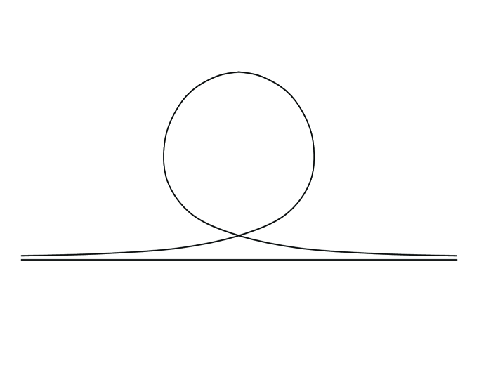
Theorem 3.7.

Let $\gamma(x,t):\mathbb{R}\times[0,\infty)\to\mathbb{R}^{2}$ be a solution of (SS) obtained by Theorem 3.6. Then there exist sequences $\{t_{j}\}^{\infty}_{j=1}$ and $\{p_{j}\}^{\infty}_{j=1}$ and a smooth proper curve $\hat{\gamma}:\mathbb{R}\to\mathbb{R}^{2}$ such that $\gamma(\cdot,t_{j})-p_{j}$ converges to $\hat{\gamma}(\cdot)$ as $t_{j}\to\infty$ up to a reparametrization. The curvature $\hat{\kappa}$ satisfies

(3.31) $$2\partial^{2}_{s}\hat{\kappa}+\hat{\kappa}^{3}-\lambda^{2}\hat{\kappa}=0$$

and

(3.32) $$\int_{\hat{\gamma}}\hat{\kappa}^{2}\,ds<\infty.$$

Moreover $\hat{\kappa}$ is given by either

(3.33) $$\hat{\kappa}\equiv 0$$

or

(3.34) $$\hat{\kappa}(s)=\begin{cases}k(s-s_{0})&\text{for}\quad s>s_{0},\\ k(-s+s_{0})&\text{for}\quad s<s_{0}\end{cases}$$

for some $s_{0}\in\mathbb{R}$, where $k(s)$ is the solution of either

(3.35) $$\begin{cases}\dfrac{dk}{ds}=-\sqrt{-\dfrac{k^{4}}{4}+\dfrac{\lambda^{2}}{2}k^{2}}\quad\text{for}\quad s\in\mathbb{R},\\ k(0)=\sqrt{2}\left|\lambda\right|\end{cases}$$

or

(3.36) $$\begin{cases}\dfrac{dk}{ds}=\sqrt{-\dfrac{k^{4}}{4}+\dfrac{\lambda^{2}}{2}k^{2}}\quad\text{for}\quad s\in\mathbb{R},\\ k(0)=-\sqrt{2}\left|\lambda\right|.\end{cases}$$

Proof.

From (3.18), it follows that $\partial^{n}_{s}\kappa(\cdot,t)$ is uniformly continuous with respect to $t$. Furthermore, the fact (3.18) implies that, as $\left|x\right|\to\infty$,

(3.37) $$\left|\partial^{n+2}_{s}\gamma(x,t)\right|\to 0,\quad\left|\partial^{n}_{s}\kappa(x,t)\right|\to 0$$

for any $t>0$. Then, along the same line as in Section 2.3, we are able to prove that

(3.38) $$\left\|\partial^{n}_{s}\partial_{t}\gamma(t)\right\|_{L^{2}_{s}}\to 0\quad\text{as}\quad t\to\infty.$$

Here we reparametrize $\gamma$ by its arc length, i.e., $\gamma=\gamma(s,t)$. Then, (3.23) implies that $\gamma(s,t)$ is defined on $[0,L]\times[0,\infty)$ for any $L\geq 2R$. In the following, let $L\geq 2R$ fix arbitrarily. For the curve $\gamma=\gamma(s,t):[0,L]\times[0,\infty)\to\mathbb{R}^{2}$, first we observe that

(3.39) $$\left|\gamma(s,t)-\gamma(0,t)\right|\leq s\leq L$$

for any $(s,t)\in[0,L]\times[0,\infty)$. Thus we see that $\gamma(s,t)-\gamma(0,t)$ is uniformly bounded with respect to $t$. It is easy to check that $\gamma(s,t)-\gamma(0,t)$ is equi-continuous with respect to $t$. Indeed, since it holds that

$$\left|\left\{\gamma(s_{1},t)-\gamma(0,t)\right\}-\left\{\gamma(s_{2},t)-\gamma(0,t)\right\}\right|\leq\left|s_{1}-s_{2}\right|,$$

if $\left|s_{1}-s_{2}\right|<\delta$, then we have

$$\left|\left\{\gamma(s_{1},t)-\gamma(0,t)\right\}-\left\{\gamma(s_{2},t)-\gamma(0,t)\right\}\right|<\varepsilon$$

for any $t>0$. Moreover, with the aid of (3.18), we verify that

$$\left|\partial^{n}_{s}\kappa(s_{1},t)-\partial^{n}_{s}\kappa(s_{2},t)\right|\leq\int^{s_{1}}_{s_{2}}\left|\partial^{n+1}_{s}\kappa(\theta,t)\right|\,d\theta<C\left|s_{1}-s_{2}\right|.$$

Therefore, by virtue of Arzelà-Ascoli’s theorem and a diagonal method, we see that there exist a sequence $\{t_{j}\}^{\infty}_{j=1}$, a planar curve $\hat{\gamma}(\cdot)$, and a function $\hat{\kappa}(\cdot)$ such that

(3.40) $$\gamma(\cdot,t_{j})-\gamma(0,t_{j})\to\hat{\gamma}(\cdot),$$

(3.41) $$\partial^{n}_{s}\kappa(\cdot,t_{j})\to\partial^{n}_{s}\hat{\kappa}(\cdot)$$

for all $n\in\mathbb{N}\cup\{0\}$ as $t_{j}\to\infty$. This implies that the curve $\hat{\gamma}(\cdot)$ is smooth and there exists a sequence $\{p_{j}\}^{\infty}_{j=1}\subset\mathbb{R}^{2}$, with $p_{j}=\gamma(0,t_{j})$, such that

$$\gamma(\cdot,t_{j})-p_{j}\to\hat{\gamma}(\cdot)$$

as $t_{j}\to\infty$. Furthermore, it follows from (3.38) and (3.41) that $\hat{\kappa}$ satisfies (3.31). Since $\gamma(s,t)$ converges to $\hat{\gamma}$ along a sequence $\{t_{j}\}^{\infty}_{j=1}$ on any compact set $[0,L]$, the estimate (3.23) yields that the limiting curve $\hat{\gamma}$ is also a smooth proper curve. Moreover (3.32) follows from (3.18) letting $t\to\infty$ along $\{t_{j}\}^{\infty}_{j=1}$.

Finally we derive a representation formula of $\hat{\kappa}$. From (3.31), we obtain

(3.42) $$\left(\dfrac{d\hat{\kappa}}{ds}\right)^{2}=-\dfrac{\hat{\kappa}^{4}}{4}+\dfrac{\lambda^{2}}{2}\hat{\kappa}^{2}+C,$$

where $C$ is an arbitrary constant. A standard theory of ordinary differential equations yields that the fact (3.32) implies $C=0$. Then it is clear that $\hat{\kappa}\equiv 0$ satisfies (3.42). If $\hat{\kappa}$ is non-trivial, then there exists a point $s=s_{0}$ such that $d\hat{\kappa}/ds$ vanishes. Therefore we obtain the conclusion. ∎

Remark 3.1.

Along the same line as in the proof of Theorem 3.7, we can also prove that, for any sequences $\{t_{j}\}_{j}$ and $\{p_{j}\}_{j}\subset\mathbb{R}^{2}$ with $p_{j}\in\gamma(\cdot,t_{j})$, there exist a subsequence $\{t_{j_{k}}\}\subset\{t_{j}\}$ and a stationary solution $\hat{\gamma}$ such that $\gamma(\cdot,t_{j_{k}})-p_{j_{k}}\to\hat{\gamma}(\cdot)$ as $t_{j_{k}}\to\infty$. Indeed, the claim is proved by applying our argument to $\gamma(\cdot,t_{j})$.

We define an index of $\gamma$ as follows:

$$i(\gamma)=\int_{\gamma}\kappa\,ds.$$

Regarding the index $i(\gamma)$, we prove that $i(\gamma)$ is invariant under the shortening-straightening flow for any finite time.

Lemma 3.6.

Let $\gamma(x,t)$ be a solution of (SS). Then $i(\gamma)$ is invariant for any finite time $t>0$.

Proof.

By virtue of Lemma 2.3, we observe that

$$\dfrac{d}{dt}i(\gamma) =\int_{\gamma}\kappa_{t}\,ds+\int_{\gamma}\kappa\,\partial_{t}ds$$

$$=-\int_{\gamma}\partial^{2}_{s}F^{\lambda}\,ds=-\left[\partial_{s}F^{\lambda}\right]^{\infty}_{-\infty}=-\left[2\partial^{3}_{s}\kappa+3\kappa^{2}\partial_{s}\kappa-\lambda^{2}\partial_{s}\kappa\right]^{\infty}_{-\infty}.$$

Since Lemma 3.4 yields that

$$\int_{\gamma}\left(\partial^{m}_{s}\kappa\right)^{2}\,ds<\infty$$

for any $m\in\mathbb{N}$ and finite time $t>0$, we see that, as $\left|x\right|\to\infty$,

$$\partial_{s}F^{\lambda}\to 0.$$

∎

With the aid of Lemma 3.6 and Remark 3.1, we can characterize a dynamical aspect of $\gamma$ starting from $\gamma_{0}$ with $i(\gamma_{0})\neq 0$.

Theorem 3.8.

Let $\gamma_{0}:\mathbb{R}\to\mathbb{R}^{2}$ be a smooth planar curve satisfying (A1)–(A4). Let $\gamma:\mathbb{R}\times[0,\infty)\to\mathbb{R}^{2}$ be a solution of (SS) obtained by Theorem 3.6. If $i(\gamma_{0})\neq 0$, then there exists at least one sequence $\{t_{j}\}_{j}$ with $t_{j}\to\infty$ such that $\gamma(\cdot,t_{j})$ converges to a borderline elastica as $t_{j}\to\infty$.

Proof.

Let $\{t_{j}\}_{j}$ be an arbitral sequence with $t_{j}\to\infty$. If $i(\gamma_{0})\neq 0$, then Lemma 3.6 implies that $\gamma(\cdot,t)$ always contains at least one loop part $l(\gamma(t))$. Let us define a sequence $\{p_{j}\}_{j}\subset\mathbb{R}^{2}$ as

(3.43) $$p_{j}\in l(\gamma(t_{j}))$$

for each $j\in\mathbb{N}$. Then, as we stated in Remark 3.1, there exist a subsequence $\{t_{j_{k}}\}\subset\{t_{j}\}$ and a stationary solution $\hat{\gamma}$ such that $\gamma(\cdot,t_{j_{k}})-p_{j_{k}}\to\hat{\gamma}(\cdot)$ as $t_{j_{k}}\to\infty$. By virtue of (3.43), the curve $\hat{\gamma}$ can not be a straight line. Therefore Theorem 3.7 gives us the conclusion. ∎

Acknowledgements

The first author was partially supported by the Fondazione CaRiPaRo Project Nonlinear Partial Differential Equations: models, analysis, and control-theoretic problems. The second author was partially supported by Grant-in-Aid for Young Scientists (B) (No. 24740097).

References

- [1] S. B. Angenent, On the formation of singularities in the curve shortening flow, J. Differential Geom. 33 (1991), no. 3, 601–633.
- [2] G. Bellettini, C. Mantegazza, and M. Novaga, Singular perturbations of mean curvature flow, J. Differential Geom. 75 (2007), 403–431.
- [3] G. Dziuk, E. Kuwert, and R. Schätzle, Evolution of elastic curves in : existence and computation, SIAM J. Math. Anal. 33 (2002), 1228–1245.
- [4] M. E. Gage, Curve shortening makes convex curves circular, Invent. Math. 76 (1984), no. 2, 357–364.
- [5] M. A. Grayson, The shape of a figure-eight under the curve shortening flow, Invent. Math. 96 (1989), no. 1, 177–180.
- [6] N. Koiso, On the motion of a curve towards elastica, Acta de la Table Ronde de Géométrie Différentielle, (1996), 403–436, Sémin. Congr. 1, Soc. Math. France, Paris.
- [7] A. Linnér, Some properties of the curve straightening flow in the plane, Trans. Amer. Math. Soc. 314 (1989), no. 2, 605–618.
- [8] A. Lunardi, Analytic Semigroup and Optimal Regularity in Parabolic Problems, Progress in Nonlinear Differential Equations and Their Applications 16 (1995), Birkhäuser.
- [9] S. Okabe, The motion of elastic planar closed curves under the area-preserving condition, Indiana Univ. Math. J. 56 (2007), no. 4, 1871–1912.
- [10] A. Polden, Curves and Surfaces of Least Total Curvature And Fourth-Order Flows, Dissertation University of Tuebingen (1996).
- [11] Y. Wen, flow of curve straightening in the plane, Duke Math. J. 70 (1993), no. 3, 683–698.
- [12] Y. Wen, Curve straightening flow deforms closed plane curves with nonzero rotation number to circles, J. Differential Equations 120 (1995), no. 1, 89–107.