Spin Magnetic Moment and Persistent Orbital Currents in Cylindrical Nanolayer

Abstract

Densities of persistent orbital and spin magnetic moment currents of an electron in a cylindrical nanolayer in the presence of external axial magnetic field are considered. For the mentioned current densities analytical expressions are obtained. The conditions when in the system only spin magnetic moment current is present are defined. Dependencies of orbital and spin magnetic moment currents on geometrical parameters of nanolayer are derived. It is shown that in the case of layered geometry the dependence of spin magnetic moment current on radial coordinate has a non-monotonic behavior. This is the peculiarity of layered geometry of nanostructure and it is due to the behavior of wave function of the system along the radial direction. Dependent on the directions of the field and orbital rotation of the electron there are defined values of radial coordinates when the orbital current disappears. The transition to the case of cylindrical quantum dot is discussed as well.

I Introduction

The development of precise methods of the growth of semiconductor nanostructures makes possible the realization of zero-dimensional systems of various geometrical forms and sizes Bimberg . As we know quantum dots (QD) are those structures where quantum effects visualize themselves more vividly. Indeed, due to the full quantization of the spectrum of charge carriers, QDs have similar properties to real atoms, hence, usually, QDs are called ”artificial atoms” Maksym_Chakraborty . They are considered to be very perspective systems that can be used as base elements for contemporary nanoelectronics: started from lasers based on QDs and finished with new generation solar cells Asryan_Luri_2001 ; Asryan_Suris_1996 ; Nozik_2002 ; Aroutiounian_Petrosyan_2001 ; Cao_Yoon_2007 . The physical processes in QDs are being investigated intensively by the specialists, because besides the pure academic interest, the results of investigation can be applicable Alferov . Currently spherical, cylindrical, ellipsoidal, pyramidal, lens-shaped and many other QDs are experimentally realized and thoroughly investigated Ozmen_Cakir ; Safar_Barati_2013 ; Chen_Xie_2013 ; Safar_Barati_2012 ; Antonov_Daniltsev_2012 ; Soylu_2012 ; Zhang_Han_2012 ; Munacute_Domin_2012 . All of these QDs listed above have specific geometries that impose their electronic, optical, kinetic and other characteristics. The latest circumstance gives a vast choice of properties of QDs for solving a concrete practical problem. An interesting class of QDs are layered QDs, for which there are two boundaries of transition from QD to the surrounding medium. This makes possible to control the physical properties of layered samples easily. In many papers it was considered electronic, optical and also thermal characteristics of ring-like and other layered nanostructures. The theoretical investigation of electron states in layered nanostructures is originated from the pioneering works of Chakraborty and Pietilainen Chak_Piet_1993 ; Chak_Piet_1994 . Authors have considered one-electron and many-electron states in quantum rings at the presence of impurities, as well as under the influence of a magnetic field. At the same time, taking into account that in the radial direction the movement of electron is restricted both on internal and external radiuses, Chakraborty and Pietilainen have suggested a model of confining potential having the form of a two-dimensional shifted oscillator. In Ref. Aghek_Kaz_2010, ; Aghek_Kaz_Kost_2011, ; Aghek_Kaz_2012, the authors have discussed one and two electronic states in spherical nanolayer with different confinement potentials. Energy spectrum and wave functions have been obtained dependent on inner and outer radiuses. Along with changing inner or outer radiuses it is also possible to control physical properties of nanolayers with external electrical and magnetic fields, with hydrostatic pressure and so on. This means that it is urgent to study such systems by investigating interband and intraband absorption coefficients, ballistic conductance of orbital and spin currents and etc. Particularly the problem of charge current in ring like structures was discussed in many papers. For example in Ref. Chak_Piet_1994, there have been studied the effect of electron-electron interaction on the magnetic moment (associated with the persistent current) of electrons in a quantum ring. There was introduced a model where the electron makes a circular motion in a parabolic confinement simulating a quantum ring which is subjected to a perpendicular magnetic field. The electron states in such a ring with and without the Coulomb interaction are then investigated. There also explored the limits of narrow and wide rings. In Ref. Nita_Marinescu_2012, it was demonstrated the theoretical possibility of obtaining a pure spin current in a 1D ring with spin-orbit interaction by irradiation with a non-adiabatic, two-component terahertz laser pulse, whose spatial asymmetry is reflected by an internal phase difference. In Ref. Castelano_2008, the persistent current in two vertically coupled quantum rings containing few electrons is studied. It was shown that the Coulomb interaction between the rings in the absence of tunneling affects the persistent current in each ring and the ground-state configurations. Quantum tunneling between the rings alters significantly the ground state and the persistent current in the system. Also this problem is discussed in Refs. Chak_Piet_1993, ; Nita_Marinescu_2011, ; Bellucci_2009, .

In general, the quantum mechanical expression for one electron current in presence of magnetic field with consideration of the spin of electron consists of two components. The first one characterizes the orbital current ${\overrightarrow{j}_{Orb}}$ and it is connected with orbital motion of the electron. The second one is caused by the magnetic moment of electron and it is called density of spin magnetic moment current - ${\overrightarrow{j}_{SMM}}$. As far as this current is not conditioned with directed motion of the electron, therefore, its divergence equals to zero:

$$div{\overrightarrow{j}_{SMM}}=0.$$

This current is specific and its existence is and is caused by the presence of the spin magnetic moment of the electron. In Ref. Mita_Bougaida_1999, the peculiarities of spin magnetic moment current were discussed, particularly, when hydrogen atom electron is in and states. In these states, the total current is formed exclusively by the spin magnetic moment current of the electron. It is interesting to note, that similar problem arises also in optics. Particularly, in Ref. Berry_2009, it is shown that for scalar light, the current is the familiar expectation value of the intensity-weighted momentum operator. Current is distinct from the local wave vector (not weighted) that could be observed by means of quantum weak measurement. For vector light, the current (Poynting vector) contains an additional term corresponding to the photon spin, recently identified for paraxial light by Bekshaev and Soskin but valid generally after a modification to restore electric-magnetic democracy this term has physical consequences. Also in Ref. Bakshaev_Bliokh_2011, it was discussed an optical phenomena associated with the internal energy redistribution which accompany propagation and transformations of monochromatic light fields in homogeneous media. The total energy flow (linear-momentum density, Poynting vector) can be divided into a spin part associated with the polarization and an orbital part associated with the spatial inhomogeneity. It is clear that in ring-like nanostructures it is also possible to discuss density of one electron current in presence of magnetic field with considering the spin. It is important to note, that in nanostructures there could be controlled densities of orbital as well as spin magnetic moment currents by the variation of geometrical parameters of studied samples.

In this paper the investigation of orbital and spin magnetic moment current densities for an electron located in cylindrical nanolayer are presented in presence of axial magnetic field.

II Cylindrical nanolayer

II.1 Energy spectrum and wave functions

Let us discuss the behavior of electron in the cylindrical nanolayer with confinement potential

$${V_{Conf}}\left({\rho,z}\right)=\left\{\begin{array}[]{l}0,\,\,{R_{1}}<\rho<{R_{2}},\,\,\left|z\right|<\frac{L}{2}\\ \infty,\,\,\rho\leq{R_{1}},\,\,\rho\geq{R_{2}},\,\,\left|z\right|\geq\frac{L}{2}\end{array}\right.,$$ (1)

where $L$ is the height of the cylindrical nanolayer, $R_{1}$ and $R_{2}$ are respectively the inner and outer radiuses (Figure 1).

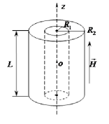
Figure 1: Geometrical shape of cylindrical nanolayer with $R_{1}$ inner and $R_{2}$ outer radiuses and $L$ height.

Let us also consider that the system is in an axial $\overrightarrow{H}$ homogenous magnetic field with the following gauge:

$$\overrightarrow{A}=\left\{{{A_{\rho}}={A_{z}}=0,{A_{\varphi}}=\frac{{H\rho}}{2}}\right\}.$$ (2)

For the gauge chosen above the variables in Schrodinger equation can be separated. By taking into account the spin of the electron one can obtain the following three dimensional equation:

$$\begin{array}[]{l}-\frac{{{\hbar^{2}}}}{{2\mu}}\left({\frac{1}{\rho}\frac{\partial}{{\partial\rho}}\left({\rho\frac{\partial}{{\partial\rho}}}\right)+\frac{{{\partial^{2}}}}{{\partial{z^{2}}}}+\frac{1}{{{\rho^{2}}}}\frac{{{\partial^{2}}}}{{\partial{\varphi^{2}}}}-\frac{{i\hbar{\omega_{H}}}}{2}\frac{\partial}{{\partial\varphi}}+\frac{{\mu\omega_{H}^{2}}}{8}{\rho^{2}}+{V_{Conf}}\left({\rho,z}\right)-{\mu^{*}}H{{\hat{\sigma}}_{z}}}\right)\psi\left({\rho,\varphi}\right)f\left(z\right){\chi_{{s_{z}}}}=\\ ={E_{{n_{z}},{n_{\rho}},m,{s_{z}}}}\psi\left({\rho,\varphi}\right)f\left(z\right){\chi_{{s_{z}}}}\end{array}$$ (3)

with the following boundary conditions:

$$\Psi{|_{z=\pm\frac{L}{2}}}=\Psi{|_{\rho={R_{1}}}}=\Psi{|_{\rho={R_{2}}}}=0$$ (4)

where $\mu^{*}$ is the effective magnetic moment of electron (for $GaAs$ ${\mu^{*}}={g_{L}}{\mu_{B}}$, ${\mu_{B}}=\frac{{e\hbar}}{{2{m_{e}}c}}$, ${g_{L}}=0,44$, ${\hat{\sigma}_{z}}$ is the $z$ component of Pauli matrices, ${\omega_{H}}=\frac{{eH}}{{\mu c}}$ is the cyclotron frequency, where $\mu=0,067{m_{e}}$, $m_{e}$ electron rest mass and ${\chi_{s}}$ is the spin part of the wave function. For the $z$ representation of Pauli matrices one can write:

$${\hat{\sigma}_{z}}=\left({\begin{array}[]{*{20}{c}}1&0\\ 0&{-1}\end{array}}\right),\,\,{\chi_{{s_{z}}=\frac{1}{2}}}=\left(\begin{array}[]{l}1\\ 0\end{array}\right)$$ (5)

Equation (3) has analytical solutions. After corresponding calculations for the wave function one can obtain the following expression:

$$\begin{split}\begin{array}[]{l}\Psi_{{n_{\rho}},m}^{n,\,{s_{z}}}\left({\rho,\varphi,z,{s_{z}}}\right)=\frac{1}{{\sqrt{2\pi}}}{e^{im\varphi}}\sqrt{\frac{2}{L}}\cdot\\ \cdot\left\{\begin{array}[]{l}\sin\frac{{\pi n}}{L}z\,(n=2k)\\ \cos\frac{{\pi n}}{L}z\,(n=2k+1)\end{array}\right\}\left(\begin{array}[]{l}1\\ 0\end{array}\right)R\left(\rho\right)\end{array}\end{split}$$ (6)

where $m=0;\pm 1;\pm 2;...$ is the magnetic quantum number.

After substitution (6) into (3) we obtain an equation for the radial wave function.After inserting the following notations:

$$\beta=\frac{{E-{E_{n}}}}{{\hbar{\omega_{H}}}}-\frac{m}{2},\,\,\\ {a_{H}}=\sqrt{\frac{\hbar}{{{\omega_{H}}\mu}}}\text{ - magnetic length}$$

the solutions for that radial equation can be written as follows:

$$R\left(\rho\right)={\rho^{\left|m\right|}}{e^{-\frac{{{\rho^{2}}}}{{4a_{H}^{2}}}}}\left\{{{C_{1}}\cdot{}_{1}{F_{1}}\left({-\left({\beta-\frac{{\left|m\right|+1}}{2}}\right),\,m+1,\,\frac{{{\rho^{2}}}}{{2a_{H}^{2}}}}\right)+{C_{2}}\cdot U\left({-\left({\beta-\frac{{\left|m\right|+1}}{2}}\right),\,m+1,\,\frac{{{\rho^{2}}}}{{2a_{H}^{2}}}}\right)}\right\}$$ (7)

where ${}_{1}{F_{1}}$ and $U$ are Kummer confluent hypergeometric and confluent hypergeometric functions correspondingly. On Figure 2 the distribution of electron probability density is depicted. As it follows from Figure 2 the maximal probability of localizing of electron is in the center of the nanolayer in radial direction. In order to find energy spectrum for the ground state, it is necessary to consider the radial boundary conditions (4) and solve the obtained transcendental equation below:

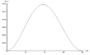
Figure 2: Distribution of density of probability of electron, when $H={10^{4}}{g^{\frac{1}{2}}}\cdot{m^{-\frac{1}{2}}}\cdot{s^{-1}}$

$$\left|\begin{array}[]{l}{}_{1}{F_{1}}\left({-\left({\beta-\frac{{\left|m\right|+1}}{2}}\right),\,m+1,\,\frac{{R_{1}^{2}}}{{2a_{H}^{2}}}}\right)\,\,\,\,\,U\left({-\left({\beta-\frac{{\left|m\right|+1}}{2}}\right),\,m+1,\,\frac{{R_{1}^{2}}}{{2a_{H}^{2}}}}\right)\\ {}_{1}{F_{1}}\left({-\left({\beta-\frac{{\left|m\right|+1}}{2}}\right),\,m+1,\,\frac{{R_{2}^{2}}}{{2a_{H}^{2}}}}\right)\,\,\,\,\,U\left({-\left({\beta-\frac{{\left|m\right|+1}}{2}}\right),\,m+1,\,\frac{{R_{2}^{2}}}{{2a_{H}^{2}}}}\right)\end{array}\right|=0$$ (8)

As a result of those operations we will get:

$${E_{n,m}}=\hbar{\omega_{H}}\left({\beta+\frac{m}{2}}\right)+{E_{n}}$$ (9)

where $\beta$ can be obtained by numerical calculations.

II.2 Orbital current

On the basis of the results obtained above one can calculate orbital and spin magnetic moment current densities for the discussed system:

$${\vec{j}_{Tot}}={\vec{j}_{Orb}}+{\vec{j}_{SMM}}$$ (10)

where the first term represents the orbital and the last one - spin magnetic moment current.

According to the theory of quantum mechanics the expression of orbital current density of a charge carrier in the magnetic field has the following form:

$${\vec{j}_{Orb}}=\frac{{ie\hbar}}{{2\mu}}\left({\Psi\vec{\nabla}{\Psi^{*}}-{\Psi^{*}}\vec{\nabla}\Psi}\right)-\frac{{{e^{2}}}}{{\mu c}}\vec{A}{\left|\Psi\right|^{2}}$$ (11)

and the spin magnetic moment current density as follows Landau_Lifshitz_2003 :

$${\vec{j}_{SMM}}={\mu^{*}}c\,rot\left({{\Psi^{*}}\hat{\vec{\sigma}}\,\Psi}\right).$$ (12)

By direct calculations it could be shown that

$$\begin{array}[]{l}{\left({{{\vec{j}}_{Orb}}}\right)_{\rho}}=0,\,\,\,{\left({{{\vec{j}}_{Orb}}}\right)_{z}}=0,\\ \,{\left({{{\vec{j}}_{Orb}}}\right)_{\varphi}}=\left({\frac{{e\hbar m}}{{\mu\rho}}-\frac{{{e^{2}}H}}{{2\mu c}}\rho}\right){\left|{\psi(\rho,\varphi)}\right|^{2}}{\left|{f(z)}\right|^{2}},\end{array}$$ (13)

Table 1:

For $m=1$

$\left|{\overrightarrow{H}}\right|({g^{\frac{1}{2}}}\cdot c{m^{\frac{1}{2}}}\cdot{s^{-2}})$	$-1.1\cdot 10^{5}$	$-1.5\cdot 10^{5}$	$-1.9\cdot 10^{5}$	$-2.3\cdot 10^{5}$	$-2.65\cdot 10^{5}$
${\rho_{m}}(\mathop{\rm A}\limits^{\circ})$	109.43	93.71	83.26	75.68	70.50

For $\left|{\overrightarrow{H}}\right|=2.65*{10^{5}}{g^{\frac{1}{2}}}*c{m^{\frac{1}{2}}}*{s^{-2}}$

$m$	1	2	3	4	5
${\rho_{m}}(\mathop{\rm A}\limits^{\circ})$	70.50	99.71	122.12	141.01	157.65

where $\psi(\rho,\varphi)$ and $f(z)$ are the two components of $\Psi$ final wave function dependent on correspondingly $\rho,\,\varphi$ and $z$ variables. The orbital current has two components. If we consider that $\hbar m$ is the orbital momentum characterizing the state with quantum number $m$, then it is clear that the first term in formula (13) characterizes the current conditioned by the orbital motion. In its turn $\frac{{eH}}{{\mu c}}$ is the cyclotron frequency of the electron. The multiplication of cyclotron frequency and $\rho$ characterizes the linear velocity of cyclotron movement of the electron. Therefore, the second term is the cyclotron frequency current and describes the contribution of the magnetic field in ${\vec{j}_{Orb}}$.

As we can see from (13), when $\frac{{e\hbar m}}{{\mu\rho}}=\frac{{{e^{2}}H}}{{2\mu c}}\rho$ correspondingly ${\rho_{m}}=\sqrt{2m}{a_{H}}$ and when radial coordinate of the electron has this value the orbital current in nanolayer becomes zero. Let us discuss it in details. As far as we consider electron so let us write this equation as $-\frac{{\left|e\right|\hbar m}}{{\mu\rho}}=\frac{{{e^{2}}H}}{{2\mu c}}\rho$. For this equation one of the following two conditions should be satisfied:

1. $m>0$ and $\overrightarrow{H}\uparrow\downarrow Oz$, which means that $\overrightarrow{H}$ has the opposite direction with respect to $Oz$ axis

2. $m<0$ and $\overrightarrow{H}\uparrow\uparrow Oz$, which, respectively, means that has the same direction as $Oz$ axis

It is important to notice that for each fixed value of $m$ there is its own fixed value of ${\rho_{m}}$ . For a given value of magnetic field $\left|{\overrightarrow{H}}\right|$ on distances equal to ${\rho_{m}}=\sqrt{2m}{a_{H}}$ orbital current equals to zero, as it was mentioned later, and when the radialcoordinate of the electron is larger than this value we have oppositelydirected orbital current. Physically this phenomenon could be explained as follows. With increasing $\rho$ the contribution of energy caused by angular momentum decreases but at the same time contribution of energy of cyclotron rotation increases. For the radiuses larger than ${\rho_{m}}$ the direction of rotation is mainly conditioned by magnetic field $\overrightarrow{H}$. On Table 1 there are shown several values of ${\rho_{m}}$ for different values of $\overrightarrow{H}$ and $m$.

In order to calculate orbital and spin magnetic moment current densities, first we should find integration constants, therefore, we should use the boundary conditions (4). Thus, for those coefficients we obtain the following expressions:

$${C_{2}}=-\frac{{{}_{1}{F_{1}}\left({-\left({\beta-\frac{{\left|m\right|+1}}{2}}\right),\,m+1,\,\frac{{{R_{1}}^{2}}}{{2a_{H}^{2}}}}\right)}}{{U\left({-\left({\beta-\frac{{\left|m\right|+1}}{2}}\right),\,m+1,\,\frac{{{R_{1}}^{2}}}{{2a_{H}^{2}}}}\right)}}{C_{1}}$$ (14)

from where, by using the normalization condition we find, that

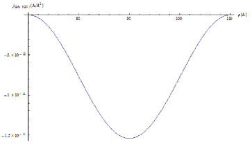
Figure 3: Dependence of orbital current density on radial coordinate for quantum cylindrical nanolayer, when $H={10^{4}}{g^{\frac{1}{2}}}\cdot{m^{-\frac{1}{2}}}\cdot{s^{-1}}$

$${C_{1}}=\frac{1}{{\sqrt{\int\limits_{{R_{1}}}^{{R_{2}}}{{\left({{\rho^{\left|m\right|}}{e^{{}^{-\frac{{{\rho^{2}}}}{{4a_{H}^{2}}}}}}}{\left[{}_{1}{F_{1}}\left({\frac{{\left|m\right|+1}}{2}-\beta,\,m+1,\,\frac{{{\rho^{2}}}}{{2a_{H}^{2}}}}\right)-\frac{{{}_{1}{F_{1}}\left({\frac{{\left|m\right|+1}}{2}-\beta,\,m+1,\,\frac{{{R_{1}}^{2}}}{{2a_{H}^{2}}}}\right)}}{{U\left({\frac{{\left|m\right|+1}}{2}-\beta,\,m+1,\,\frac{{{R_{1}}^{2}}}{{2a_{H}^{2}}}}\right)}}U\left({\frac{{\left|m\right|+1}}{2}-\beta,\,m+1,\,\frac{{{\rho^{2}}}}{{2a_{H}^{2}}}}\right)\right]}\right)}^{2}}\rho d\rho}}}$$ (15)

On Figure 3 the dependence of orbital current density on radial coordinate for the ground state of electron ($n=1,m=0$) is illustrated. Let us discuss the behavior of these current densities in detail when $L=500\text{\AA}$, $R_{1}=70\text{\AA}$, $R_{2}=110\text{\AA}$. In Figure 3 it can be seen that the modulus of orbital current density fully repeats the radial distribution of the electron in the nanolayer and that is natural. As far as we consider the state when $m=0$, the orbital current is negative and its profile has the inverted form of density of probability of radial distribution.

II.3 Spin magnetic moment current

Now let us turn to the investigation of spin magnetic moment current. As for the spin magnetic moment current density calculation, first it is necessary to calculate the components of the following vector:

$$\bar{\vec{\sigma}}={\mu^{*}}{\Psi^{*}}\hat{\vec{\sigma}}\,\Psi$$ (16)

By taking into consideration the forms of Pauli matrices and ${\chi_{s}}$ wave function, with direct calculations it can be obtained that

$${\left({\bar{\vec{\sigma}}}\right)_{\rho}}={\left({\bar{\vec{\sigma}}}\right)_{\varphi}}=0$$ (17)

and

$${\left({\bar{\vec{\sigma}}}\right)_{z}}=2{\mu^{*}}{s_{z}}{\left|\psi\right|^{2}}{\left|f\right|^{2}}.$$ (18)

$\left({{{\left|\psi\right|}^{2}}{{\left|f\right|}^{2}}}\right)$ multiplication is only dependent on $\rho$ and $z$ coordinates, therefore different from zero will be only the $\varphi$ component of $rot\bar{\vec{\sigma}}$. For $\rho,\varphi$ and $z$ components of spin magnetic moment current density one can obtain:

$$\begin{gathered}{\left({{{\vec{j}}_{SMM}}}\right)_{\rho}}=0,\,\,{\left({{{\vec{j}}_{SMM}}}\right)_{\varphi}}=-2{\mu^{*}}c{s_{z}}\frac{\partial}{{\partial\rho}}{\left|\psi\right|^{2}}{\left|f\right|^{2}},\\ {\left({{{\vec{j}}_{SMM}}}\right)_{z}}=0.\end{gathered}$$ (19)

Finally, for the total current density it can be written:

$$\begin{gathered}{\left({{{\vec{j}}_{tot}}}\right)_{\varphi}}=\left({\frac{{e\hbar m}}{{\mu\rho}}-\frac{{{e^{2}}H}}{{2\mu c}}\rho}\right){\left|\psi\right|^{2}}{\left|f\right|^{2}}-\\ -2{\mu^{*}}c{s_{z}}\frac{\partial}{{\partial\rho}}{\left|\psi\right|^{2}}{\left|f\right|^{2}}.\end{gathered}$$ (20)

These results are quite expected because in $\rho$ and $z$ directions charge carriers motion is limited. On the other hand we have periodical rotation of particle around $Oz$ axis which creates cyclical current.

It should be noted, that in contrast with the case of quantum wire, the consideration of the quantization along the $Oz$ axis leads to the vanishing of the orbital current in the direction of magnetic field. On the other hand both in orbital and in spin magnetic moment current expressions the presence of $Oz$ direction is expressed by the presence of ${\left|f\right|^{2}}$ factor. Therefore, dependent on which $z=const$ plain is discussed the current, for the same $\rho$ it will have different values. It is important to note that, in the expression of total current ${\left({{{\vec{j}}_{tot}}}\right)_{\varphi}}$ the factor ${\left|f\right|^{2}}$ characterizes the quantization along $Oz$ axis. Herewith

$${\left|f\right|^{2}}=\left\{\begin{array}[]{l}\frac{2}{L}{\sin^{2}}\left({\frac{{\pi n}}{L}z}\right)\left({n-even}\right)\\ \frac{2}{L}{\cos^{2}}\left({\frac{{\pi n}}{L}z}\right)\left({n-odd}\right)\end{array}\right.$$ (21)

Hence, along $Oz$ axis of cylindrical nanolayer there are plains where total current equals to zero (see Figure 4). These plains match to ${\left|f\right|^{2}}$ factor zeros. Let us consider two cases: one for an even value of and another for an odd one. For example, when $n=6$ we should consider ${\left|f\right|^{2}}=\frac{2}{L}{\sin^{2}}\left({\frac{{\pi n}}{L}z}\right)$.Then there will be seven flats where total current will be equal to zero. $z$ coordinates of these plains could be calculated from $\frac{2}{L}{\sin^{2}}\left({\frac{{6\pi}}{L}z}\right)=0$ condition. For the case of $n=7$ (the odd case) zero plains are obtained by the same calculations for ${\left|f\right|^{2}}=\frac{2}{L}{\cos^{2}}\left({\frac{{\pi n}}{L}z}\right)$. These results could be illustrated as follows:

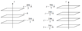
Figure 4: Illustration of plains where total current equals to zero.

One more important thing that should be noted: by fixing $m$ in expression (20) one can choose the magnetic vector $\overrightarrow{H}$ so that in the total current density the contribution would have only the spin magnetic moment current:

$${\left({{{\vec{j}}_{tot}}}\right)_{\varphi}}=-2{\mu^{*}}c{s_{z}}{\left|f\right|^{2}}\left\{{\frac{{\partial{{\left|\psi\right|}^{2}}}}{{\partial\rho}}}\right\}.$$ (22)

which is conditioned by the gradient of electron radial distribution.

On Figure 5 and 6 spin magnetic moment and total current densities are depicted respectively. As we can see on Figure 5 spin magnetic moment has a non-monotonic character. Such behavior is specific for the layered geometries. As far as $\overrightarrow{\nabla},\overrightarrow{{\mu^{*}}}$ and ${\overrightarrow{j}_{SMM}}$ form a right-handed orthogonal trio, from (12) it follows that when $\overrightarrow{\nabla}{\left|\psi\right|^{2}}$ changes its direction to opposite ${\overrightarrow{j}_{SMM}}$ should change its direction to opposite too (see Figure 7).

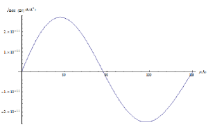
Figure 5: Dependence of spin magnetic moment current density on radial coordinate for quantum cylindrical nanolayer, when $H={10^{4}}{g^{\frac{1}{2}}}\cdot{m^{-\frac{1}{2}}}\cdot{s^{-1}}$

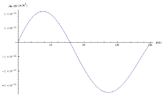
Figure 6: Dependence of total current density on radial coordinate for quantum cylindrical nanolayer, when $H={10^{4}}{g^{\frac{1}{2}}}\cdot{m^{-\frac{1}{2}}}\cdot{s^{-1}}$

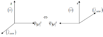
Figure 7: Right-handed orthogonal trio of the vectors.

In fact, the spin magnetic moment current is a pseudo current. Here under the spin magnetic moment current it must be understood imaginary currents which would create the same magnetic field distribution which is created by the spin magnetic moment of the electron. From physical point of view it is obvious that for the cylindrical nanolayer the spin magnetic moment should create a magnetic field parallel to the axis of the cylindrical nanolayer as the spin was directed by the axis originally. A magnetic field parallel to $Oz$ axis can be caused by oppositely directed currents in a plain perpendicular to the $Oz$ axis (Figure 5).

III Cylindrical quantum dot

Let us also discuss the case of quantum cylinder, i. e. the limiting case when the inner radius of the cylindrical nanolayer is equal to zero. All the logic and calculations are the same as that for cylindrical nanolayer with only one difference: radial wave function has the following form Atayan_Kazaryan_2008

$$R\left(\rho\right)={C_{3}}{\rho^{\left|m\right|}}{e^{-\frac{{{\rho^{2}}}}{{4a_{H}^{2}}}}}{}_{1}{F_{1}}\left({\frac{{\left|m\right|+1}}{2}-\beta,\,\left|m\right|+1,\,\frac{{{\rho^{2}}}}{{2a_{H}^{2}}}}\right)$$ (23)

where $\beta=\frac{{{E_{\rho}}}}{{\hbar{\omega_{H}}}}+sign(e)\frac{m}{2}$. Again, by using the normalization condition we can find the integration constant and from boundary condition $R\left({{\rho_{0}}}\right)=0$, where $\rho_{0}$ is the cylinder radius, we can find the energy spectrum. Thereby, we obtain that Atayan_Kazaryan_2008

$${\alpha_{{n_{\rho}}+1,\left|m\right|}}=\beta-\frac{{\left|m\right|+1}}{2}$$

where ${n_{\rho}}=0;\,\,1;\,\,2;\,\,...$. Hence,

$${E_{{n_{\rho}},m}}=\hbar{\omega_{H}}\left({{\alpha_{{n_{\rho}}+1,m}}-sign\left(e\right)\frac{m}{2}+\frac{{\left|m\right|+1}}{2}}\right).$$ (24)

It should be mentioned, that these solutions are entirely analogous to the ones of non-diffracting Laguerre-Gaussian optical beams Bliokh_Schattschneider_2012 .

On Figure 8 the distribution of probability density of electron dependent on radial coordinate for the case of cylindrical quantum dot is depicted.

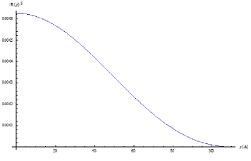
Figure 8: Distribution of electron density of probability for cylindrical QD, when $H={10^{4}}{g^{\frac{1}{2}}}\cdot{m^{-\frac{1}{2}}}\cdot{s^{-1}}$

On Figure 9 it is shown the dependence of orbital current on radial coordinate. As we can see on periphery and in the center of the cylinder the current is equal to zero. On the periphery it equals to zero because wave function, and, therefore, the probability of electron localization there becomes zero. In the center of the system the current is equal to zero because there is no rotation of the electron.

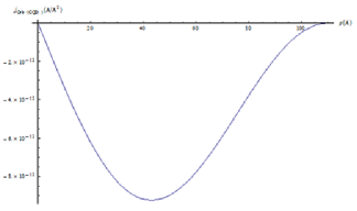
Figure 9: Dependence of orbital current density on radial coordinate for cylindrical QD, when $H={10^{4}}{g^{\frac{1}{2}}}\cdot{m^{-\frac{1}{2}}}\cdot{s^{-1}}$

As for the spin magnetic moment current densities the behavior is shown on Figure 10 from where we can see

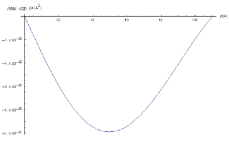
Figure 10: Dependence of spin magnetic moment current density on radial coordinate for cylindrical QD, when $H={10^{4}}{g^{\frac{1}{2}}}\cdot{m^{-\frac{1}{2}}}\cdot{s^{-1}}$

that we have current with spatial distribution of electron charge similar to the orbital current density. As in the case of cylindrical nanolayer we can say as far as we consider the state when $m=0$, the orbital current is negative and its profile has the inverted form of density of probability of radial distribution.

On Figure 11 the dependence of total current on radial coordinate is illustrated.

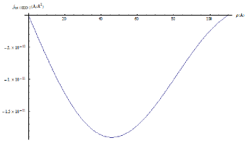
Figure 11: Dependence of total current on radial coordinate for cylindrical QD, when $H={10^{4}}{g^{\frac{1}{2}}}\cdot{m^{-\frac{1}{2}}}\cdot{s^{-1}}$

IV Conclusion

Thereby, in this paper the orbital and spin magnetic moment currents of an electron in a cylindrical nanolayer are investigated. Analytical expressions are obtained for both of those currents. It was shown that under certain conditions the main contribution to the total current is due to the spin magnetic moment current. Particularly, there are cylindrical surfaces parallel to the axis of the nanolayer, where the orbital current becomes zero. It was shown that there are plains perpendicular to the axis of the nanolayer, where both the persistent orbital and spin magnetic moment currents become zero.

Also the calculations were done for the limiting case when the inner radius of the nanolayer is zero. It was illustrated that the spin magnetic moment current has non-monotonic behavior in the radial direction, whereas in the case of cylindrical QD it has monotonic character. Both for the cylindrical nanolayer and for cylindrical QD it was shown that the persistent orbital and spin magnetic moment current can be controlled by changing the geometrical parameters of the quantum nanostructures - the inner or outer radius in the case of the layer, and the radius in the case of the QD.

V Acknowledgements

The authors thank Professor Konstantin Bliokh for useful discussions. The work was performed as a part of the basic program of state of the Republic of Armenia ”Studies of the physical properties of quantum nanostructures with complex geometries and different limiting potentials”.

VI References

References

- (1) D. Bimberg, M. Grundmann, Ledentsov, Quantum dot heterostructures, 1999, Wiley, New York.
- (2) P.A. Maksym, T. Chakraborty, Quantum dots in a magnetic field: Role of electron-electron interactions, Physical Review Letters, vol. 65, 1990.
- (3) L.V. Asryan, S. Luryi, Tunneling-injection quantum-dot laser: ultrahigh temperature stability, Journal of Quantum Electronics, vol. 37, no. 7, 2001.
- (4) L.V. Asryan, R. Suris, Inhomogeneous line broadening and the threshold current density of a semiconductor quantum dot laser, Semiconductor Science and Technology, vol. 11, no. 4, 1996.
- (5) A. Nozik, Quantum dot solar cells, Physica E, vol. 14, no. 1-2, 2002.
- (6) V. Aroutiounian, S. Petrosyan, A. Khachatryan, K.Touryan, Quantum dot solar cells, Journal of Applied Physics, Journal of Applied Physics, vol. 89, no. 4, pp. 2268-2271, 2001.
- (7) Q. Cao, S.F. Yoon, C.Y. Liu, C.Y Ngo, Narrow ridge waveguide high power single mode 1.3-m InAs/InGaAs ten-layer quantum dot lasers, Nanoscale Research Letters, vol. 2, no. 6, pp. 303-307, 2007.
- (8) Z. Alferov, The history and future of semiconductor heterostructures, Semiconductors, vol. 32, no. 1, pp. 1-14, 1998.
- (9) A. Özmen, B. Çakir, Y. Yakar, Electronic structure and relativistic terms of one-electron spherical quantum dot, Journal of Luminescence, vol. 137, 2013.
- (10) Gh. Safarpour, M. Barati, The optical absorption coefficient and refractive index changes of aspherical quantum dot placed at the center of a cylindrical nano-wire, Journal of Luminescence, vol. 137, 2013.
- (11) T. Chen, W. Xie, Sh. Liang, Optical and electronic properties of a two-dimensional quantum dot with an impurity, Journal of Luminescence, vol. 139, 2013.
- (12) Gh. Safarpour, M. Barati, M. Moradi, Electron-hole transition in a spherical quantum dot confined at the center of a cylindrical nano-wire: Comparison of isotropic and anisotropic effective mass, Superlattices and Microstructures, vol. 52, no. 4, 2012.
- (13) A.V. Antonov, V.M. Daniltsev, M.N. Drozdov, Yu.N. Drozdov, L.D. Moldavskaya, V. I. Shashkin, Intraband photoconductivity induced by interband illumination in InAs/GaAs heterostructures with quantum dots, Semiconductors, vol. 46, no. 11, 2012.
- (14) A. Soylu, The influence of external fields on the energy of two interacting electrons in a quantum dot, Annals of Physics, vol. 327, no. 12, 2012.
- (15) Y. Zhang, X. Han, J. Zhang, Y. Liu, H. Huang, H. Ming, Sh. Lee, Zh. Kang, Photoluminescence of silicon quantum dots in nanospheres, Nanoscale, vol. 4, no. 24, 2012.
- (16) J. Munrriz, F. Domnguez-Adame, P.A. Orellana, A.V. Malyshev, Graphene nanoring as a tunable source of polarized electrons, Nanotechnology, vol. 23, no. 20, 2012.
- (17) T. Chakraborty, P. Pietilinen, Interacting-electron states and the persistent current in a quantum ring, Solid State Communications, vol. 87, no. 9, pp. 809-812, 1993.
- (18) T. Chakraborty, P. Pietilinen, Electron-electron Interaction and the Persistent Current in a Quantum Ring, Physical Review B (Condensed Matter), vol. 50, no. 12, pp. 8460-8468, 1994.
- (19) N. G. Aghekyan, E. M. Kazaryan and H. A. Sarkisyan, Two Electron States in a Thin Spherical Nanolayer: Reduction to the Model of Two Electrons on a Sphere, Few-Body Systems, vol. 53, no. 3-4, pp. 505-513, 2012.
- (20) N.G. Aghekyan, E.M. Kazaryan, A.A. Kostanyan, H.A. Sarkisyan, Two electronic states and state exchange time control in spherical nanolayer, Superlattices and Microstructures, vol. 50, no. 3, pp. 199-276, 2011.
- (21) N. G. Aghekyan ; E. M. Kazaryan ; A. A. Kostanyan ; H. A. Sarkisyan, Two electronic states in spherical quantum nanolayer, Proceedings of SPIE, pp. 7998, 79981C, 2010.
- (22) Niţǎ M., Marinescu D. C., Ostahie B., Manolescu A., Gudmundsson V., Nonadiabatic generation of spin currents in a quantum ring with Rashba and Dresselhaus spin-orbit interactions, Journal of Physics: Conference Series, vol. 338, no. 1, 2012.
- (23) L.K. Castelano, G.-Q. Hai, B. Partoens, F.M. Peeters, Correlated persistent currents in a stack of semiconductor quantum rings, Physical Review B, vol. 77, no. 19, p. 235314, 2008.
- (24) M. Niţǎ, D. C. Marinescu, A. Manolescu, V. Gudmundsson, Non-adiabatic generation of a pure spin current in a 1D quantum ring with spin-orbit interaction, Physical Review B, vol. 83, no. 15, p. 155427, 2011.
- (25) S. Bellucci, P. Onorato, Quantum rings with tunnel barriers in a threading magnetic field: Spectra, persistent current and ballistic conductance, Physica E: Low-dimensional Systems and Nanostructures, vol. 41, no. 8, p. 1393-1402, 2009.
- (26) K. Mita, M. Boufaida, Ideal capacitor circuits and energy conservation, American Journal of Physics, vol. 67, no. 8, p. 737, 1999.
- (27) M. Berry, Optical currents, Journal of Optics A: Pure and Applied Optics, Journal of Optics A: Pure and Applied Optics, vol. 11, no. 9, 2009.
- (28) A. Bekshaev, K.Y. Bliokh, M. Soskin, Internal flows and energy circulation in light beams, Journal of Optics, vol. 13, no. 5, 2011.
- (29) L. D. Landau, L.M. Lifshitz, Quantum Mechanics: Non-Relativistic Theory, Third Edition: Volume 3 Moscow, 2003.
- (30) A.K. Atayan, E.M. Kazaryan, A.V. Meliksetyan, H.A. Sarkisyan, Magneto-absorption in cylindrical quantum dots, The European Physical Journal B, vol. 63, no. 4, pp. 485-492, 2008.
- (31) K. Bliokh, P. Schattschneider, J. Verbeeck, F. Nori, Electron Vortex Beams in a Magnetic Field: A New Twist on Landau Levels and Aharonov-Bohm States, Physical Review X, vol. 2, Issue 4, id. 041011, 2012.