Re-entrant Disordered Phase in a System of Repulsive Rods on a Bethe-like Lattice

Abstract

We solve exactly a model of monodispersed rigid rods of length $k$ with repulsive interactions on the random locally tree like layered lattice. For $k\geq 4$ we show that with increasing density, the system undergoes two phase transitions: first from a low density disordered phase to an intermediate density nematic phase and second from the nematic phase to a high density re-entrant disordered phase. When the coordination number is $4$, both the phase transitions are continuous and in the mean field Ising universality class. For even coordination number larger than $4$, the first transition is discontinuous while the nature of the second transition depends on the rod length $k$ and the interaction parameters.

I Introduction

A system of long hard rods in three dimensions undergoes a phase transition from a disordered phase with no orientational order to an orientationally ordered nematic phase as the density of rods is increased beyond a critical value Onsager (1949); Flory (1956); Zwanzig (1963), and has applications in the theory of liquid crystals Vroege and Lekkerkerker (1992); de Gennes and Prost (1993). In two dimensions, though an ordered phase that breaks a continuous symmetry is disallowed Mermin and Wagner (1966), the system undergoes a Kosterlitz-Thouless type transition from an isotropic phase with exponential decay of orientational correlation to a high density critical phase Straley (1971); Frenkel and Eppenga (1985); Khandkar and Barma (2005); Vink (2009). On two-dimensional lattices, remarkably, there are two entropy driven transitions for long rods: first from a low density disordered (LDD) phase to an intermediate density nematic phase, and second from the nematic phase to a high density disordered (HDD) phase Ghosh and Dhar (2007). While the existence of the first transition has been proved rigorously Disertori and Giuliani (2012), the second transition has been demonstrated only numerically Kundu et al. (2013). In this paper, we consider a model of rods interacting via a repulsive potential on the random locally tree like layered lattice, and through an exact solution show the existence of two phase transitions as the density is varied.

We describe the lattice problem in more detail. Rods occupying $k$ consecutive lattice sites along any lattice direction will be called $k$-mers. No two $k$-mers are allowed to intersect, and all allowed configurations have the same energy. For dimers ($k$ = 2), it is known that the system remains disordered at all packing densities Heilmann and Lieb (1972). For $k\geq k_{min}$, it was argued that the system of hard rods would undergo two phase transitions as density is increased Ghosh and Dhar (2007). On both the square and the triangular lattices $k_{min}=7$ Ghosh and Dhar (2007); Matoz-Fernandez et al. (2008a). Monte Carlo studies show that the first transition from LDD phase to nematic phase is continuous, and is in the Ising universality class for the square lattice and in the three-state Potts model universality class for the triangular lattice Matoz-Fernandez et al. (2008b, c, a); Linares et al. (2008); Fischer and Vink (2009). The existence of this transition has been has been proved rigorously for large $k$ Disertori and Giuliani (2012). The second transition from nematic to HDD phase was studied using an efficient algorithm that ensures equilibration of the system at densities close to full packing Kundu et al. (2012, 2013). On the square lattice the second transition is continuous with effective critical exponents that are different from the two dimensional Ising exponents, though a crossover to the Ising universality class at larger length scales could not be ruled out Kundu et al. (2013). On the triangular lattice the second transition is continuous and the critical exponents are numerically close to those of the first transition. This raises the question whether the LDD and HDD phases are same or different.

Is there a solvable model of $k$-mers that shows two transitions with increasing density and throws light on the HDD phase? The hard core $k$-mer problem was solved exactly on the random locally tree like layered lattice (RLTL), a Bethe-like lattice Dhar et al. (2011). This lattice was introduced because a uniform nematic order is unstable on the more conventional Bethe lattice when the coordination number is larger than $4$. However, on the RLTL, while a stable nematic phase exists for all even coordination numbers greater than or equal to four, the second transition is absent for hard rods Dhar et al. (2011). In this paper, we relax the hard-core constraint and allow $k$-mers of different orientations to intersect at a lattice site. Weights $u,v,\ldots$ are associated with sites that are occupied by two, three, $\ldots$ $k$-mers. When the weights are zero, we recover the hard rod problem. We solve this model on the RLTL and show that for a range of $u,v,\ldots$, the system undergoes two transitions as the density is increased: first from a LDD phase to a nematic phase and second from the nematic phase to a HDD phase. For coordination number $q=4$, the two transitions are continuous and belong to the mean field Ising universality class. For $q\geq 6$, where $q$ is an even integer, while the first transition is first order, the second transition is first order or continuous depending on the values of $k,u,v,\ldots.$. In all cases, it is possible to continuously transform the LDD phase into the HDD phase in the $\rho$–interaction parameters phase diagram without crossing any phase boundary, showing that the LDD and HDD phases are qualitatively similar, and hence the HDD phase is a re-entrant LDD phase.

The rest of the paper is organized as follows. In Sec. II, we recapitulate the construction of RLTL and formulate the model of rods on this lattice. In Sec  III, we derive the analytic expression for free energy for fixed density of horizontal and vertical $k$-mers on the $4$-coordinated RLTL. It is shown that the system undergoes two continuous phase transitions for $k\geq 4$. In Sec. IV, the free energy is computed for coordination number $q=6$, and the dependence of the nature of the transition on the different parameters are detailed. Sec. V summarizes the main results of the paper, and discusses some possible extensions.

II The RLTL and definition of the model

The RLTL was introduced in Ref. Dhar et al. (2011). In this section, we recapitulate its construction for coordination number $q=4$. Generalization to larger even values of $q$ is straightforward. Consider a collection of $M$ layers, each having $N$ sites. A layer $m$ is connected to its adjacent layer ($m-1$) by $N$ bonds of type $X$ and $N$ bonds of type $Y$. Each site in the $m^{th}$ layer is connected with exactly one randomly chosen site in the $(m-1)^{th}$ layer with a bond of type $X$. Similarly bonds of type $Y$ are also connected by random pairing of sites in the two adjacent layers. Hence, the total number of such possible pairing between two layers is $(N!)^{2}$. A typical bond configuration is shown in Fig. 1. For a $q$-coordinated lattice with periodic boundary conditions, the total number of different possible graphs is $(N!)^{qM/2}$, and with open boundary conditions there are $(N!)^{q(M-1)/2}$ different possible graphs. In the thermodynamic limit, the RLTL contains few short loops and locally resembles a Bethe lattice.

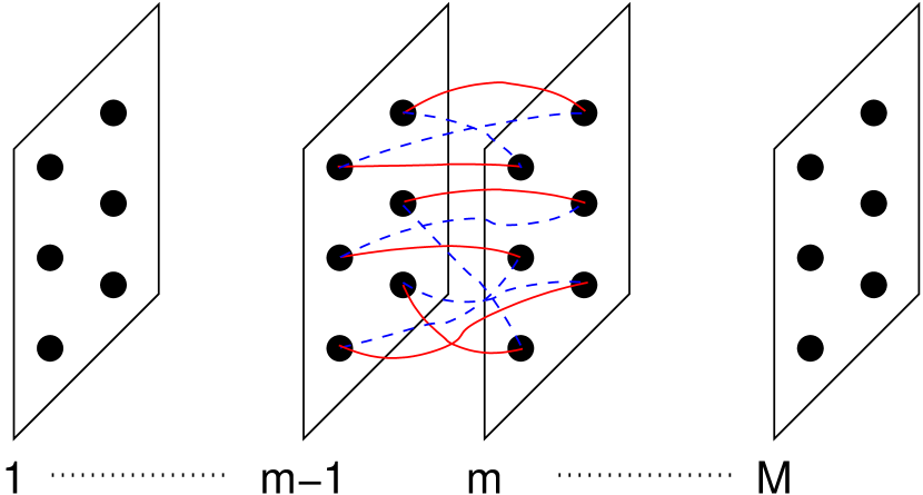
Figure 1: Schematic diagram of the RLTL with $N=6$ sites per layer and coordination number $4$. A typical bond configuration between layers $m-1$ and $m$ is shown with $X$ bonds in red (solid) lines and $Y$ bonds in blue (dotted) lines.

We consider a system of monodispersed rods of length $k$ on the RLTL. A $k$-mer occupies $(k-1)$ consecutive bonds of same type. Rods on $X$ ($Y$) type of bonds will be called $x$-mers ($y$-mers). Weights $e^{\mu_{1}}$ and $e^{\mu_{2}}$ are associated with each $x$-mer and $y$-mer, where $\mu$’s are chemical potentials. Linear rods comprising of $k$ monomers are placed on the RLTL such that a site can be occupied by utmost two $k$-mers. Two $k$-mers of the same type can not intersect. A weight $u$ is associated with every site that is occupied by two $k$-mers of different type. The limiting case $u=0$ corresponds to the hard core problem. For even $q\geq 6$, a site can be occupied by utmost $q/2$ $k$-mers, each of different type.

Consider the annealed model on RLTL. The average partition function is

$$Z_{av}(M,N)=\frac{1}{N_{\mathcal{R}}}\sum_{\mathcal{R}}Z_{\mathcal{R}}(M,N),$$ (1)

where $Z_{\mathcal{R}}(M,N)$ is the partition function for a given bond configuration $\mathcal{R}$ and $N_{\mathcal{R}}$ is the number of different bond configurations on the lattice. In the thermodynamic limit the mean free energy per site is obtained by

$$f=-\lim_{M,N\to\infty}\frac{1}{MN}\ln Z_{av},$$ (2)

where the temperature and Boltzmann constant have been set equal to $1$.

III $k$-mers on RLTL with coordination number $4$

In this section, we calculate the free energy of the system on the RLTL of coordination number $4$ for fixed $u$ and fixed densities of $x$-mers and $y$-mers. The phase diagram of the system is obtained by minimizing the free energy with respect to $x$-mer and $y$-mer densities for a fixed total density.

III.1 Calculation of Free energy

To calculate the partition function, consider the operation of adding the $m^{th}$ layer, given the configuration up to the $(m-1)^{th}$ layer. The number of ways of adding the $m^{th}$ layer is denoted by $C_{m}$. $C_{m}$ will be a function of the number of $x$-mers and $y$-mers passing through the $m^{th}$ layer and the number of intersections between $x$-mers and $y$-mers at the $m^{th}$ layer.

Let $x_{m}$ $(y_{m})$ be the number of $x$-mers ($y$-mers) whose left most sites or heads are in the $m^{th}$ layer. $X_{m}$ and $Y_{m}$ are the number of sites in the $m^{th}$ layer occupied by $x$-mers and $y$-mers respectively, but where the site is not the head of the $k$-mer. Clearly,

$$X_{m}=\sum_{j=1}^{k-1}x_{m-j},~{}Y_{m}=\sum_{j=1}^{k-1}y_{m-j},~{}1\leq m\leq M,$$ (3)

with $x_{m}=y_{m}=0$, for $m\leq 0$. To have all $k$-mer fully contained with in the lattice for open boundary condition we need to impose, $x_{m}=y_{m}=0$ for, $m\geq M-k+2$.

In a $k$-mer, let $h$ denote its head or left most site and $b$ denote the other $k-1$ sites. Then, we define $\Gamma^{m}_{ij}$, where $i,j=h,b$, to be the number of intersections at the $m^{th}$ layer between site $i$ of an $x$-mer and site $j$ of a $y$-mer. For instance, $\Gamma^{m}_{hh}$ is the number of sites in the $m^{th}$ layer, occupied simultaneously by the heads of an $x$-mer and a $y$-mer.

Given $\{x_{m}\}$, $\{y_{m}\}$ and $\{\Gamma^{m}_{ij}\}$, the calculation of $C_{m}$ reduces to an enumeration problem. The details of the enumeration are given in appendix A. We obtain

$$C_{m} = \frac{N!X_{m}!Y_{m}!(N-X_{m})!(N-Y_{m})!}{(x_{m}-\Gamma^{m}_{hh}-\Gamma^{m}_{hb})!(y_{m}-\Gamma^{m}_{hh}-\Gamma^{m}_{bh})!(X_{m}-\Gamma^{m}_{bb}-\Gamma^{m}_{bh})!(Y_{m}-\Gamma^{m}_{bb}-\Gamma^{m}_{hb})!}$$ (4)

$$\times\frac{1}{\left(N-X_{m}-Y_{m}-x_{m}-y_{m}+\displaystyle\sum_{i,j=b,h}\Gamma^{m}_{ij}\right)!\displaystyle\prod_{i,j=b,h}\Gamma^{m}_{ij}!}.$$

The partition function is then the weighted sum of the product of $C_{m}$ for different layers:

$$Z_{av} = \frac{1}{(N!)^{2M}}\sum_{\{x_{m}\},\{y_{m}\},\{\Gamma^{m}_{ij}\}}$$ (5)

$$\prod_{m}\left(C_{m}e^{\mu_{1}x_{m}}e^{\mu_{2}y_{m}}u^{\sum_{ij}\Gamma^{m}_{ij}}\right).$$

where the sum is over all possible number of $x$-mers, $y$-mers and number of doubly occupied sites. Since the summand is of order $\exp(NM)$, for large $N,M$, we replace the summation with the largest summand with negligible error. For the summand to be maximum with respect to $x_{l}$, we set:

$$\frac{C(\{x_{m}+\delta_{m,l}\},\{y_{m}\},\{\Gamma^{m}_{ij}\})e^{\mu_{1}}}{C(\{x_{m}\},\{y_{m}\},\{\Gamma^{m}_{ij}\})}\approx 1,$$ (6)

where $C=\prod_{m}C_{m}$. Likewise, we can write equations for each of the variables.

We look for homogeneous solutions such that $\rho_{x}=x_{m}k/N$, $\rho_{y}=y_{m}k/N$, and $\gamma^{m}_{ij}=\Gamma_{ij}/N$ are variables that are independent of $N$ and have no spatial dependence. Here $\rho_{x}$ and $\rho_{y}$ are fractions of sites in any layer that are occupied by $x$-mers and $y$-mers respectively. In terms of these variables, Eq. (6) and the corresponding one for $y_{j}$ reduce to

$$\frac{(\rho_{x}-\frac{\rho_{x}}{k})^{k-1}(1-\rho\!+\!\sum_{ij}\!\!\gamma_{ij})^{k}(\frac{\rho_{x}}{k}\!-\!\gamma_{hh}\!-\!\gamma_{hb})^{-1}}{(1-\rho_{x}+\frac{\rho_{x}}{k})^{k-1}(\rho_{x}-\frac{\rho_{x}}{k}-\gamma_{bb}-\gamma_{bh})^{k-1}}=e^{-\mu_{1}},$$ (7)

and

$$\frac{(\rho_{y}-\frac{\rho_{y}}{k})^{k-1}(1-\rho\!+\!\sum_{ij}\!\!\gamma_{ij})^{k}(\frac{\rho_{y}}{k}\!-\!\gamma_{hh}\!-\!\gamma_{bh})^{-1}}{(1-\rho_{y}+\frac{\rho_{y}}{k})^{k-1}(\rho_{y}-\frac{\rho_{y}}{k}-\gamma_{bb}-\gamma_{hb})^{k-1}}=e^{-\mu_{2}},$$ (8)

where $\rho=\rho_{x}+\rho_{y}$ is the total density. On maximizing the summand in Eq. (5) with respect to $\Gamma^{l}_{ij}$, we obtain

$$\frac{[\rho_{x}(1\!\!-\!\frac{1}{k}\!)\!-\!\gamma_{bb}\!-\!\!\gamma_{bh}][\rho_{y}(1\!\!-\!\frac{1}{k}\!)\!-\!\gamma_{bb}\!-\!\!\gamma_{hb}]}{\gamma_{bb}(1-\rho+\sum_{ij}\gamma_{ij})} = \frac{1}{u},$$ (9a)

$$\frac{(\frac{\rho_{x}}{k}-\gamma_{hh}-\gamma_{hb})(\frac{\rho_{y}}{k}-\gamma_{hh}-\gamma_{bh})}{\gamma_{hh}(1-\rho+\sum_{ij}\gamma_{ij})} = \frac{1}{u},$$ (9b)

$$\frac{(\frac{\rho_{x}}{k}-\gamma_{hh}-\gamma_{hb})[\rho_{y}(1-\frac{1}{k})-\gamma_{bb}-\gamma_{hb}]}{\gamma_{hb}(1-\rho+\sum_{ij}\gamma_{ij})} = \frac{1}{u},$$ (9c)

$$\frac{(\frac{\rho_{y}}{k}-\gamma_{hh}-\gamma_{bh})[\rho_{x}(1-\frac{1}{k})-\gamma_{bb}-\gamma_{bh}]}{\gamma_{bh}(1-\rho+\sum_{ij}\gamma_{ij})} = \frac{1}{u},$$ (9d)

where $i,j=h,b$. Equation (9) can easily be solved to express $\gamma_{bb}$, $\gamma_{hb}$ and $\gamma_{bh}$ in terms of $\gamma_{hh}$:

$$\gamma_{bb}=(k-1)^{2}\gamma_{hh},~{}\gamma_{bh}=\gamma_{hb}=(k-1)\gamma_{hh},$$ (10)

and $\gamma_{hh}$ satisfies the quadratic equation

$$\gamma_{hh}^{2}-\gamma_{hh}\frac{\rho-\rho u-1}{k^{2}(1-u)}-\frac{u\rho_{x}\rho_{y}}{k^{4}(1-u)}=0.$$ (11)

From Eq. (5), the free energy is calculated using Eq. (2). We express the free energy in terms of $\rho_{x}$, $\rho_{y}$ and $u$ as

$$f(\rho_{x},\rho_{y},u) = -\frac{k-1}{k}\sum_{i}\rho_{i}\ln\rho_{i}-\sum_{i}\left[1-\frac{(k-1)\rho_{i}}{k}\right]\ln\left[1-\frac{(k-1)\rho_{i}}{k}\right]+\sum_{i}(\rho_{i}-k^{2}\gamma_{hh})\ln(\rho_{i}-k^{2}\gamma_{hh})$$ (12)

$$+(1-\rho+k^{2}\gamma_{hh})\ln(1-\rho+k^{2}\gamma_{hh})-\frac{\rho}{k}\ln k+k^{2}\gamma_{hh}\ln\left(\frac{k^{2}\gamma_{hh}}{u}\right),$$

where $\gamma_{hh}$ is a function of $\rho_{x}$, $\rho_{y}$ and $u$ through Eq. (11). This expression for the free energy is not convex everywhere. The true free energy $\bar{f}(\rho_{x},\rho_{y},u)$ is obtained by the Maxwell construction such that

$$\bar{f}(\rho_{x},\rho_{y},u)=\mathcal{CE}\left[f(\rho_{x},\rho_{y},u)\right],$$ (13)

where $\mathcal{CE}$ denotes the convex envelope. Given total density $\rho$, the minimum of free energy determines $\rho_{x}$ and $\rho_{y}$.

III.2 Two Phase Transitions

To study the phase transitions we define the nematic order parameter as

$$\psi=\frac{\rho_{x}-\rho_{y}}{\rho}.$$ (14)

The free energy can then be expressed as a power series in $\psi$,

$$f(\rho_{x},\rho_{y},u)=A_{0}(\rho,u)+A_{2}(\rho,u)\psi^{2}+A_{4}(\rho,u)\psi^{4}+\ldots,$$ (15)

where the coefficient $A_{4}(\rho,u)>0$. $f(\rho_{x},\rho_{y},u)$ is unchanged when $\psi\leftrightarrow-\psi$. For small densities, the coefficient of the quadratic terms $A_{2}(\rho,u)$ is positive and the free energy has a minimum at $\psi=0$ corresponding to the LDD phase. However for $k\geq 4$, if $u$ is smaller than a critical value $u_{c}$, then $A_{2}(\rho,u)$ changes sign continuously at a critical density $\rho_{c1}$ and the free energy has two symmetric minima at $\psi\neq 0$, corresponding to the nematic phase. This qualitative change in the behavior of the free energy for densities close to $\rho_{c1}$ is shown in Fig. 2. As density is further increased, $A_{2}(\rho,u)$ changes sign continuously from negative to positive at a second critical density $\rho_{c2}$, such that the free energy has a minimum at $\psi=0$, corresponding to the HDD phase. The dependence of the free energy on $\psi$ for densities close to $\rho_{c2}$ is similar to that shown in Fig. 2.

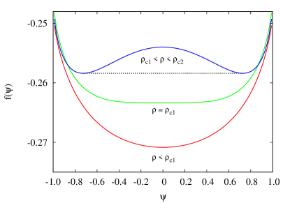
Figure 2: Free energy $f(\psi)$ as a function of the order parameter $\psi$ for $\rho\approx\rho_{c1}$. The data are for $k=6$, $u=0.15$, and $q=4$. The curves have been shifted for clarity. The dotted line denotes the convex envelope.

The variation of the order parameter $\psi$ with density $\rho$ is shown in Fig. 3 for different values of $u$. $\psi$ increases continuously from zero at $\rho_{c1}$ and decreases continuously to zero at $\rho_{c2}$. The average number of intersections between the rods per site, though continuous, also shows non-analytic behavior at $\rho_{c1}$ and $\rho_{c2}$ (see Fig. 4). The power series expansion of free energy in Eq. (15) has the same form as that of a system with scalar order parameter that has two broken symmetry phases. Thus, the two transitions will be in the mean field Ising universality class. The nematic phase does not exist for $k<4$.

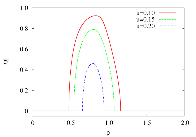
Figure 3: Order parameter $\psi$ as a function of density $\rho$. For low and high densities, $\psi=0$, while for intermediate densities, $\psi\neq 0$. The data are for $q=4$ and $k=6$.

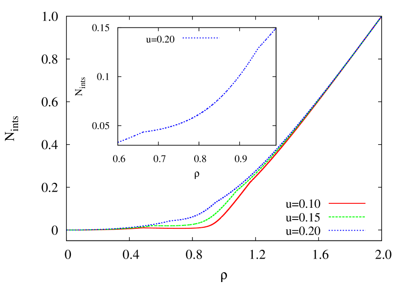
Figure 4: Average number of interactions per site, $N_{ints}$, as a function of density $\rho$ for different values of $u$. Inset: The region between the two critical points is magnified. The data are for $q=4$ and $k=6$.

The phase diagram in the $\rho$–$u$ plane is determined by solving $A_{2}(\rho,u)=0$ for $\rho$ and is shown in Fig. 5 for different values of $k$. The difference between the two critical densities decreases with increasing $u$. Beyond a maximum value $u_{c}(k)$, there is no phase transition and the system remains disordered at all densities. The critical densities $\rho_{c1}$ and $\rho_{c2}$ may be solved as an expansion in $u$. For example, when $k=4$,

$$\rho_{c1}=\frac{2}{k-1}+2u+12u^{2}+O(u^{3}),~{}~{}k=4.$$ (16)

and

$$\rho_{c2}=1.13148-2.38675u-12.2726u^{2}+O(u^{3}),~{}k=4.$$ (17)

It is of interest to determine $\rho_{c2}$ for large $k$. For the hard rod problem, it was conjectured that $\rho_{c2}\approx 1-a/k^{2}$, when $k\rightarrow\infty$ Ghosh and Dhar (2007). For our model, we find,

$$\rho_{c2} = \frac{-1+2k-\sqrt{-3+4k}}{-1+k},~{}~{}u\rightarrow 0,$$ (18)

$$= 2-\frac{2}{\sqrt{k}}+\frac{1}{k}-\frac{5}{4k^{3/2}}+\frac{1}{k^{2}}+O(k^{-5/2}).$$

Thus the leading correction is $O(1/\sqrt{k})$, and not $O(1/k^{2})$.

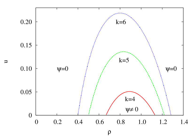
Figure 5: Phase diagram when $q=4$ for different values of $k$.

$u_{c}(k)$, the largest value of $u$ for which the nematic phase exists, is determined by solving the equations $A_{2}(\rho,u)=0$ and $dA_{2}(\rho,u)/d\rho=0$ simultaneously. $u_{c}(k)$ increases with $k$ (see Fig. 6), and approaches $1$ from below as $k\rightarrow\infty$. At $u_{c}(k)$ two mean-field Ising critical lines meet.

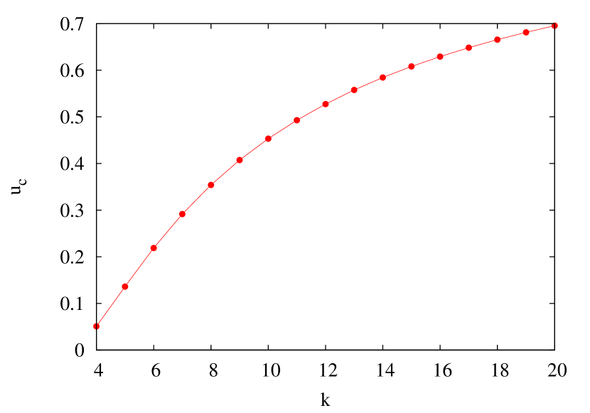
Figure 6: $u_{c}$, the maximum value of $u$ for which the transitions exists as a function of $k$. The data are for $q=4$.

IV $k$-mers on RLTL with $q=6$

The calculation presented in Sec. III may be extended to the case when the coordination number $q\geq 6$. We discuss the results when $q=6$. In this case, we associate a weight $u$ $(v)$ to a site occupied by two (three) $k$-mers of different type. The calculation of the free energy now involves many more combinatorial factors than for the case $q=4$, but is straightforward. The details of the calculation may be found in Supplementary material supplement . Let $\rho_{x}$, $\rho_{y}$ and $\rho_{z}$ be the fraction of sites occupied by $x$-mers, $y$-mers and $z$-mers respectively. We define the order parameter to be $\psi=(\rho_{x}-\rho_{y})/\rho$, where we set $\rho_{y}=\rho_{z}$. We find that for $u<u_{c}(k)$ and $v<u$, the system undergoes two transitions as for the case $q=4$, at critical densities $\rho_{c1}$ and $\rho_{c2}$.

The three dimensional $\rho$–$u$–$v$ phase diagram may be visualized by studying the phase diagram along three different lines in the $u$–$v$ plane: $v=u^{2}$, $v=u^{3}$ and $v=u^{4}$. The free energy, expressed as a power series in $\psi$, now has the form

$$f(\rho_{x},\rho_{y},u,v) = A_{0}(\rho,u,v)+A_{2}(\rho,u,v)\psi^{2}$$ (19)

$$+ A_{3}(\rho,u,v)\psi^{3}+A_{4}(\rho,u,v)\psi^{4}+\ldots,$$

where $A_{4}(\rho,u,v)>0$ and $A_{3}(\rho,u,v)$ is in general non-zero. At low densities, $A_{2}(\rho,u,v)$ is positive and the free energy has a global minimum at $\psi=0$. With increasing density it develops a second local minimum at $\psi\neq 0$. At $\rho_{c1}$ the two minima become degenerate, and for $\rho_{c1}<\rho<\rho_{c2}$, the free energy has a minimum at $\psi\neq 0$, corresponding to the nematic phase. A typical example is shown in Fig. 7. The order parameter thus shows a discontinuity at $\rho_{c1}$ and the transition is first order. In all the cases we have studied, we find that the first transition from disordered to nematic phase is discontinuous.

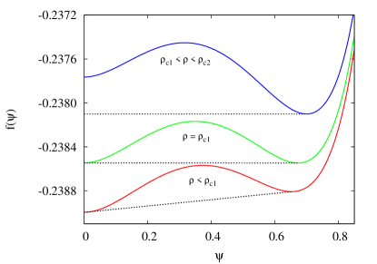
Figure 7: Free energy $f(\psi)$ as a function of the order parameter $\psi$ for $\rho\approx\rho_{c1}$ when $q=6$. The data are for $k=6$, $v=u^{2}$ and $u=0.15$. The dotted lines denote the convex envelopes.

On the other hand, the nature of the second transition from the nematic to HDD phase depends on the value of $k$, $u$ and $v$. When $v=u^{2}$, the second transition is first order for all $k$. However, when $v=u^{3}$, the second transition could be first order or continuous. We find that for $k<7$, the second transition is always first order. For $k=7$, the variation of the order parameter $\psi$ with density $\rho$ is shown in Fig. 8. Qualitatively similar behavior is seen for $k>7$. The second transition is continuous for $u\leq u^{*}(k)$ and first order for $u>u^{*}(k)$. The value of $u^{*}(k)$ increases with $k$. When $v=u^{4}$, the phenomenology is qualitatively similar to that for the case $v=u^{3}$.

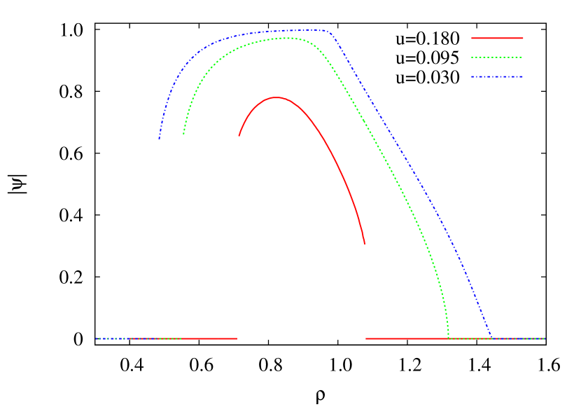
Figure 8: Order parameter $\psi$ as a function of density $\rho$ for different values of $u$ for $k=7$, $q=6$, and $v=u^{3}$. The second transition is first order for $u>u^{*}(k)$ and continuous for $u\leq u^{*}(k)$. Here $u^{*}(7)\approx 0.09563$.

The first order or continuous nature of the second transition is also reflected in the average number of intersections. In Fig. 9, we show the variation for the number of intersections per site with density for $k=7$ for two values of $u$: one corresponding to a first order and the other to continuous transition. In addition to $\psi$, the average number of intersections between rods per site also shows a discontinuity when the transition is first order. This discontinuity vanishes when the transition becomes continuous.

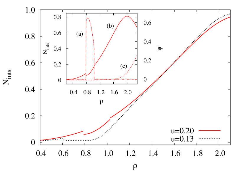
Figure 9: The number of interactions per site, $N_{ints}$, as a function of density $\rho$ for two different values of $u$. The data are for $q=6$, $k=7$, and $v=u^{4}$. Inset: The variation with density of (a) order parameter $\psi$, (b) fraction of sites occupied by two $k$-mers, and (c) fraction of sites occupied by three $k$-mers. Here, $u=0.20$.

These observations are summarized in the $\rho$–$u$ phase diagram for $k=7$ shown in Fig. 10. For $v=u^{3}$ and $v=u^{4}$, a second order line terminates at a tricritical point beyond which the transition becomes first order.

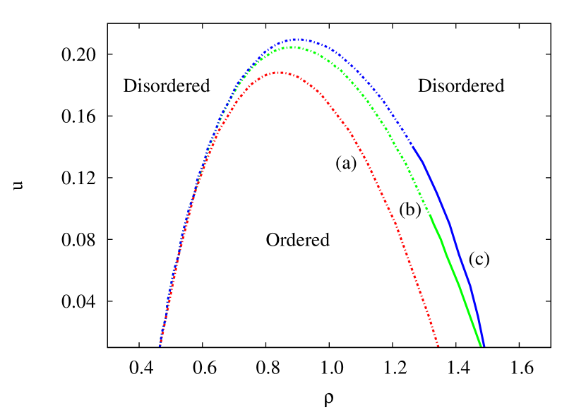
Figure 10: Phase diagram for $q=6$ and $k=7$ for (a) $v=u^{2}$, (b) $v=u^{3}$, and (c) $v=u^{4}$. Dotted (solid) lines denotes first (second) order transitions.

The exponents describing the continuous transitions may be found from the Landau-type free energy, Eq. (19). At the first transition $A_{2}(\rho,u,v)>0$ and $A_{3}(\rho,u,v)<0$. At the spinodal point $A_{2}(\rho,u,v)$ changes sign to negative. As density is further increased $A_{2}(\rho,u,v)$ changes sign back to positive. When this occurs, $A_{3}(\rho,u,v)$ could be positive or negative. If positive, then the transition will be continuous. Now the critical exponents are determined from a Landau free energy functional of the form $A_{2}\psi^{2}+A_{3}\psi^{3}$, and hence the critical exponent $\beta=1$, where $\psi\sim(\rho_{c2}-\rho)^{\beta}$ as $\rho$ approaches $\rho_{c2}$ from below. At the tricritical point $A_{3}(\rho,u,v)=0$, and the transition is in the mean field Ising universality class with $\beta=1/2$ (see Fig. 11).

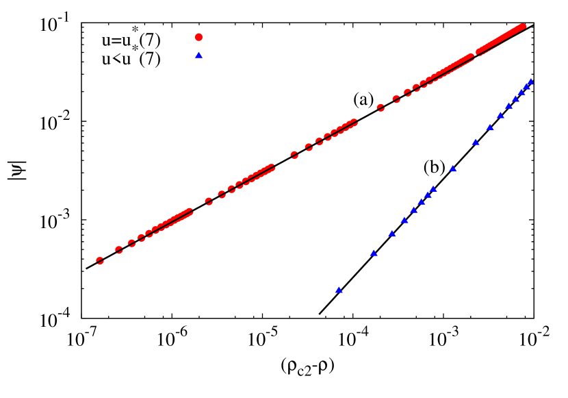
Figure 11: The order parameter $\psi$ as the density $\rho$ approaches the critical density $\rho_{c2}$ for $u<u^{*}$ and at the tricritical point $u=u^{*}$ when $k=7$, $q=6$ and $v=u^{3}$. The solid lines are power laws (a) $(\rho_{c2}-\rho)^{1/2}$ and (b) $(\rho_{c2}-\rho)$.

V Summary and Discussion

In this paper, we studied the problem of monodispersed long rigid rods on the RLTL, a Bethe-like lattice where rods of different orientations are allowed to intersect with weight $u,v,\ldots$ depending on whether a site is occupied by two, three, $\ldots$ $k$-mers. We showed that the system undergoes two phase transitions with increasing density for $k\geq k_{min}$ and appropriate choice of interaction parameters. For coordination number $q=4$, the two transitions are continuous and in the mean field Ising universality class. For $q=6$, while the first transition is first order, the nature of the second transition depends on the values $k$, $u$ and $v$, giving rise to a rich phase diagram. To the best of our knowledge, it is the only solvable model on interacting rods that shows two phase transitions.

The limit $u\to 0$ is different from $u=0$ (the hard rod problem). When $u=0$, the second transition in absent Dhar et al. (2011). When $u,v>0$, the fully packed phase is disordered by construction and if the first phase transition exists, so does a second phase transition. The relaxation of the restriction that only rods of different orientations may intersect at a lattice site does not change the qualitative behavior of the system as the high density phase remains disordered. There are still two transitions, both in the mean field Ising universality class (when $q=4$). However, the solution becomes more cumbersome.

Similarly when $q=6$, the limit $v\rightarrow 0$ is different from $v=0$ when $u>0$. When $v=0$, a lattice site may occupied by utmost two $k$-mers of different type. In this case, the fully packed phase is not necessarily disordered and for certain values of $k$ and $u$, only one transition is present for increasing density.

For hard rods on the square lattice, Monte Carlo simulations were unable to give a clear answer to the question whether the HDD and LDD phases are qualitatively similar or not Kundu et al. (2013). It was argued that the HDD phase has a large crossover length scale $\xi^{*}$ $\sim 1500$, and for length scales larger than $\xi^{*}$ it is possible that the HDD phase is not qualitatively different from the LDD phase. This was based on the evidence that vacancies in the HDD phase do not form a bound state. In this paper, by expanding the phase diagram from a one-dimensional $\rho$ phase diagram to a multi-dimensional $\rho$–interaction parameters phase diagram, we showed that it is always possible to continuously transform the LDD phase into the HDD phase without crossing any phase boundary. This means that the LDD and HDD phases are qualitatively similar, at least for the model on RLTL. It would thus be worthwhile to simulate the hard rods problem on the square lattice for system sizes larger than $1500$ and verify the same.

It would also be possible to study the problem with repulsive interactions on the square lattice. The algorithm presented in Refs. Kundu et al. (2012, 2013) is generalizable to the case when intersections are allowed. Confirming whether the qualitative behavior is similar to that seen for RLTL would be interesting. Measuring the exponents for the second transition might be easier for such a model as the critical density would be away from the fully packed limit.

For the RLTL with coordination number $q=4$, we showed that for large $k$, $\rho_{c2}\approx 2-a/\sqrt{k}+O(k^{-1})$. This is at variance from the prediction from entropy based arguments for the hard rod problem that $\rho_{c2}$ approaches $1$ as $k^{-2}$ Ghosh and Dhar (2007). It would be interesting to resolve this discrepancy.

The RLTL is suitable for studying problems that show orientational order. Polydispersed systems can show multiple phases Speranza and Sollich (2003b); Fasolo and Sollic (2003). Its solution on the RLTL would make rigorous some of the qualitative features of the problem. This is a promising area for future study.

Appendix A Calculation of $C_{m}$ for $q=4$

In this appendix, we derive the expression for $C_{m}$ in Eq. (4). $C_{m}$ is the total number of ways of connecting the bonds from the $(m-1)^{th}$ layer to the $m^{th}$ layer consistent with the number of $x$-mers, $y$-mers, and intersections at the $m^{th}$ layer.

In the $(m-1)^{th}$ layer, there are $X_{m}$ and $Y_{m}$ sites occupied by $x$-mers and $y$-mers that extend to the $m^{th}$ layer. These $X_{m}$ bonds of type $X$ can be connected to $X_{m}$ different sites in the $m^{th}$ layer in

$$\frac{N!}{(N-X_{m})!}$$

ways. Among the $Y_{m}$ bonds of type $Y$, $\Gamma^{m}_{bb}$ of them are connected to sites occupied by an $x$-mer and the remaining $Y_{m}-\Gamma^{m}_{bb}$ bonds are connected to empty sites in the $m^{th}$ layer. The number of ways of connecting is

$$\frac{Y_{m}!X_{m}!}{\Gamma^{m}_{bb}!(Y-\Gamma^{m}_{bb})!(X_{m}-\Gamma^{m}_{bb})!}\times\frac{(N-X_{m})!}{(N-X_{m}-Y_{m}+\Gamma^{m}_{bb})!}.$$

Now connect the remaining $(N-X_{m})$ free bonds of type $X$ and $(N-Y_{m})$ free bonds of type $Y$ to sites in layer $m$ that are not occupied by $x$-mers and $y$-mers respectively. This can be done in

$$(N-X_{m})!(N-Y_{m})!$$

ways.

We have to now assign sites to $x_{m}$ and $y_{m}$ heads in layer $m$. Out of $x_{m}$ ($y_{m}$) heads, $\Gamma_{hb}^{m}$ ($\Gamma_{bh}^{m}$) of them will be on sites already occupied by only a $y$-mer ($x$-mer). The number of ways of doing this is

$$\frac{(X_{m}-\Gamma^{m}_{bb})!}{\Gamma^{m}_{bh}!(X_{m}-\Gamma^{m}_{bb}-\Gamma^{m}_{bh})!}\times\frac{(Y_{m}-\Gamma^{m}_{bb})!}{\Gamma^{m}_{hb}!(Y_{m}-\Gamma^{m}_{bb}-\Gamma^{m}_{hb})!}.$$

There are $(N-X_{m}-Y_{m}+\Gamma^{m}_{bb})$ sites in the $m^{th}$ layer which are unoccupied so far. They can be divided into four groups: $\Gamma^{m}_{hh}$ sites, each occupied by the heads of an $x$-mer and a $y$-mer, $(x_{m}-\Gamma^{m}_{hh}-\Gamma^{m}_{hb})$ sites occupied by only a head of an $x$-mer, $(y_{m}-\Gamma^{m}_{hh}-\Gamma^{m}_{bh})$ sites occupied by only a head of a $y$-mer, and $(N-X_{m}-Y_{m}-x_{m}-y_{m}+\sum_{ij}\Gamma^{m}_{ij})$ unoccupied sites. The number of ways of arranging them is:

$$\begin{split}\frac{(N-X_{m}-Y_{m}+\Gamma^{m}_{bb})!}{\Gamma^{m}_{hh}!(x_{m}-\Gamma^{m}_{hh}-\Gamma^{m}_{hb})!(y_{m}-\Gamma^{m}_{hh}-\Gamma^{m}_{bh})!}\\ \times\frac{1}{(N-X_{m}-Y_{m}-x_{m}-y_{m}+\sum_{ij}\Gamma^{m}_{ij})!}.\end{split}$$

The product of all these factors gives $C_{m}$ as given in Eq. (4).

References

- Onsager (1949) L. Onsager, Ann. N.Y. Acad. Sci. 51, 627 (1949).
- Flory (1956) P. J. Flory, Proc. R. Soc. 234, 60 (1956).
- Zwanzig (1963) R. Zwanzig, J. Chem. Phys. 39, 1714 (1963).
- Vroege and Lekkerkerker (1992) G. J. Vroege and H. N. W. Lekkerkerker, Rep. Prog. Phys. 55, 1241 (1992).
- de Gennes and Prost (1993) P. G. de Gennes and J. Prost, The Physics of Liquid Crystals (Oxford University Press, Oxford, 1993).
- Mermin and Wagner (1966) N. D. Mermin and H. Wagner, Phys. Rev. Lett. 17, 1133 (1966).
- Straley (1971) J. P. Straley, Phys. Rev. A 4, 675 (1971).
- Frenkel and Eppenga (1985) D. Frenkel and R. Eppenga, Phys. Rev. A 31, 1776 (1985).
- Khandkar and Barma (2005) M. D. Khandkar and M. Barma, Phys. Rev. E 72, 051717 (2005).
- Vink (2009) R. L. C. Vink, Euro. Phys. J. B 72, 225 (2009).
- Ghosh and Dhar (2007) A. Ghosh and D. Dhar, Euro. Phys. Lett. 78, 20003 (2007).
- Disertori and Giuliani (2012) M. Disertori and A. Giuliani, arXiv:1112.5564, to appear on Comm. Math. Phys. (2013).
- Kundu et al. (2013) J. Kundu, R. Rajesh, D. Dhar, and J. F. Stilck, Phys. Rev. E 87, 032103 (2013).
- Heilmann and Lieb (1972) O. J. Heilmann and E. Lieb, Commun. Math. Phys. 25, 190 (1972).
- Matoz-Fernandez et al. (2008a) D. A. Matoz-Fernandez, D. H. Linares, and A. J. Ramirez-Pastor, J. Chem. Phys. 128, 214902 (2008a).
- Matoz-Fernandez et al. (2008b) D. A. Matoz-Fernandez, D. H. Linares, and A. J. Ramirez-Pastor, Euro. Phys. Lett 82, 50007 (2008b).
- Matoz-Fernandez et al. (2008c) D. A. Matoz-Fernandez, D. H. Linares, and A. J. Ramirez-Pastor, Physica A 387, 6513 (2008c).
- Linares et al. (2008) D. H. Linares, F. Romá, and A. J. Ramirez-Pastor, J. Stat. Mech. , P03013 (2008).
- Fischer and Vink (2009) T. Fischer and R. L. C. . Vink, Euro. Phys. Lett. 85, 56003 (2009).
- Kundu et al. (2012) J. Kundu, R. Rajesh, D. Dhar, and J. F. Stilck, AIP Conf. Proc. 1447, 113 (2012).
- Dhar et al. (2011) D. Dhar, R. Rajesh, and J. F. Stilck, Phys. Rev. E 84, 011140 (2011).
- (22) see Supplementary Material
- Speranza and Sollich (2003b) A. Speranza and P. Sollich, Phys. Rev. E 67, 061702 (2003b).
- Fasolo and Sollic (2003) M. Fasolo and P. Sollich, Phys. Rev. Lett. 91, 068301 (2003).