Three dimensional evolution of SN 1987A in a self-gravitating disk.

Abstract

The introduction of a exponential or power law gradient in the interstellar medium (ISM) allows to produce an asymmetric evolution of the supernova remnant (SNR) when the framework of the thin layer approximation is adopted. Unfortunately both the exponential and power law gradients for the ISM do not have a well defined physical meaning. The physics conversely is well represented by an isothermal self-gravitating disk of particles whose velocity is everywhere Maxwellian. . We derived a law of motion in the framework of the thin layer approximation with a control parameter of the swept mass. The photon’s losses ,that are often neglected in the thin layer approximation, are modeled trough a velocity dependence. The developed framework is applied to SNR 1987A and the three observed rings are simulated.

Keywords: supernovae: general supernovae: individual (SN 1987A ) ISM : supernova remnants

1 Introduction

The expansion of supernova remnant (SNR) is usually explained by the theory of the shock waves, as an example [1, 2] analyzes self-similar solutions with varying inverse power law exponents for the density profile of the advancing matter, $R^{-n}$, and ambient medium, $R^{-s}$. The SNRs conversely often present a weak departure from the circular symmetry, as an example in SN  1006  a ratio of 1.2 between maximum and minimum radius has been measured, see [3] or great asymmetry as the triple ring of SN  1987A  , see [4, 5].

The asymmetries of SNRs are hardly explained by the shock theory which is usually developed in spherical or planar symmetry. The presence of gradients in the density of the medium allows to explain such asymmetries when the conservation of the momentum is adopted. As an example an exponential decay allows to model SN  1006  and SN  1987A , see [6]. At the same time the various gradients that can be adopted such as Gaussian,power law and exponential do not have a precise physical basis. The auto-gravitating Maxwellian medium provides a gradient given by the secant law. In this paper we will answer the following questions.

• Is it possible to deduce an analytical formula for the temporal evolution of an SN in the presence of a vertical profile density as given by an ISD?

• Is it possible to deduce an equation of motion for SN with an adjustable parameter that can be found from a numerical analysis of the diameter–time relationship?

• Is it possible to simulate the appearance of the triple ring system of SN  1987A  ?

2 A modified thin layer approximation

The thin layer approximation with non cubic dependence (NCD) , $p$ , in classical physics assumes that only a fraction of the total mass enclosed in the volume of the expansion accumulates in a thin shell just after the shock front. The global mass between $0$ and $R_{0}$ is $\frac{4}{3}\pi\rho R_{0}^{3}$ where $\rho$ is the density of the ambient medium. The swept mass included in the thin layer which characterizes the expansion is

$$M_{0}=(\frac{4}{3}\pi\rho R_{0}^{3})^{\frac{1}{p}}\quad.$$ (1)

The mass swept between $0$ and $R$ is

$$M=(\frac{4}{3}\pi\rho R^{3})^{\frac{1}{p}}\quad.$$ (2)

The conservation of radial momentum requires that, after the initial radius $R_{0}$,

$$MV=M_{0}V_{0}\quad,$$ (3)

where $R$ and $V$ are the radius and velocity of the advancing shock. The velocity is

$$V=V_{0}(\frac{M_{0}}{M})^{\frac{1}{p}}\quad.$$ (4)

The velocity as a function of the radius when the expansion starts at the origin of the coordinates is:

$$V=V_{0}(\frac{R_{0}}{R})^{\frac{3}{p}}\quad.$$ (5)

The velocity can be expressed as

$$V=\frac{dR}{dt}\quad,$$ (6)

and the integration between $R$ , $t$ and $R_{0}$ , $t_{0}$ gives

$$p{R}^{1+3\,{p}^{-1}}\left(3+p\right)^{-1}-p{R_{{0}}}^{1+3\,{p}^{-1}}\left(3+p\right)^{-1}=V_{{0}}{R_{{0}}}^{3\,{p}^{-1}}\left(t-t_{{0}}\right)\quad.$$ (7)

We solve the previous equation for $R$ and we obtain

$$R(t)=$$

$$\left({R_{{0}}}^{1+3\,{p}^{-1}}+\left(3+p\right)V_{{0}}{R_{{0}}}^{3\,{p}^{-1}}\left(t-t_{{0}}\right){p}^{-1}\right)^{{\frac{p}{3+p}}}\quad.$$ (8)

The velocity is:

$$V=\frac{N}{D}$$ (9)

$$where$$

$$N=$$

$$({{\it R_{0}}}^{1+3\,{p}^{-1}}+(3+p)\,$$

$$\,{\it V_{0}}\,{{\it R_{0}}}^{3\,{p}^{-1}}(t-{\it t_{0}}){p}^{-1})^{{\frac{p}{3+p}}}{\it V_{0}}\,{{\it R_{0}}}^{3\,{p}^{-1}}p$$

$$D={{\it R_{0}}}^{1+3\,{p}^{-1}}p+3\,{\it V_{0}}\,{{\it R_{0}}}^{3\,{p}^{-1}}t+{\it V_{0}}\,{{\it R_{0}}}^{3\,{p}^{-1}}tp$$

$$-3\,{\it V_{0}}\,{{\it R_{0}}}^{3\,{p}^{-1}}{\it t_{0}}-{\it V_{0}}\,{{\it R_{0}}}^{3\,{p}^{-1}}{\it t_{0}}\,p\,.$$

Equation (8) can also be solved with a solution of type $R=K(t-t_{0})^{\alpha}$, $k$ being a constant, and the asymptotic result is:

$$R(t)=\left(\frac{\left(3+p\right)V_{{0}}{R_{{0}}}^{3/p}\left(t-t_{{0}}\right)}{p}\right)^{{\frac{p}{3+p}}}\quad.$$ (10)

The asymptotic solution for the velocity is

$$V(t)=$$

$$\left(3+p\right)^{-\frac{3}{3+p}}{p}^{\frac{3}{3+p}}{{\it V_{0}}}^{{\frac{p}{3+p}}}{{\it R_{0}}}^{\frac{3}{3+p}}\left(t-{\it t_{0}}\right)^{-\frac{3}{3+p}}\quad.$$ (11)

3 Asymmetrical law of motion with NCD

Given the Cartesian coordinate system $(x,y,z)$, the plane $z=0$ will be called the equatorial plane, $z=R\sin(\theta)$, where $\theta$ is the latitude angle which has range $[-90^{\circ}\leftrightarrow+90^{\circ}]$, and $R$ is the distance from the origin. In our framework, the polar angle of the spherical coordinate system is $90-\theta$. Here we adopt the density profile of a thin self-gravitating disk of gas which is characterized by a Maxwellian distribution in velocity and distribution which varies only in the z-direction (ISD). The number density distribution is

$$n(z)=n_{0}sech^{2}(\frac{z}{2\,h})\quad,$$ (12)

where $n_{0}$ is the density at $z=0$, $h$ is a scaling parameter and $sech$ is the hyperbolic secant ([7, 8]). On assuming that the expansion starts at $z\approx 0$ , we can write $z=R\sin(\theta)$ and therefore

$$n(R,\theta)=n_{0}sech^{2}(\frac{R\sin(\theta)}{2\,h})\quad,$$ (13)

where $R$ is the radius of the advancing shell.

The 3D expansion that starts at the origin of the coordinates will be characterized by the following properties

• Dependence of the momentary radius of the shell on the polar angle $\theta$ that has a range $[-90^{\circ}\leftrightarrow+90^{\circ}]$.

• Independence of the momentary radius of the shell from $\phi$ , the azimuthal angle in the x-y plane, that has a range $[0^{\circ}\leftrightarrow 360^{\circ}]$.

The mass swept, $M$, along the solid angle $\Delta\;\Omega$, between 0 and $R$ is

$$M(R)=\frac{\Delta\;\Omega}{3}m_{H}n_{0}I_{m}(R)+\frac{4}{3}\pi R_{0}^{3}n_{0}m_{H}\quad,$$ (14)

where

$$I_{m}(R)=\int_{R_{0}}^{R}r^{2}sech^{2}(\frac{r\sin(\theta)}{2\,h})dr\quad,$$ (15)

where $R_{0}$ is the initial radius and $m_{H}$ the mass of the hydrogen. The integral is

$$I_{m}(R)=$$

$$-4\,h{r}^{2}(\sin(\theta))^{-1}(1+{{\rm e}^{{\frac{r\sin(\theta)}{h}}}})^{-1}+4\,{\frac{h{r}^{2}}{\sin(\theta)}}$$

$$-8\,{h}^{2}r\ln(1+{{\rm e}^{{\frac{r\sin(\theta)}{h}}}})(\sin(\theta))^{-2}$$ (16)

$$-8\,{h}^{3}{\it\mathrm{Li}_{2}\/}(-{{\rm e}^{{\frac{r\sin(\theta)}{h}}}})(\sin(\theta))^{-3}\quad,$$ (17)

where

$$\mathop{\mathrm{Li}_{2}\/}\nolimits\!\left(z\right)=\sum_{{n=1}}^{\infty}\frac{z^{n}}{n^{2}}\quad,$$ (18)

is the dilogarithm, see [9, 10, 11].

The conservation of the momentum gives

$$(M(R))^{\frac{1}{p}}\dot{R}=(M(R_{0}))^{\frac{1}{p}}\dot{R_{0}}\quad,$$ (19)

where $\dot{R}$ is the velocity at $R$ and $\dot{R_{0}}$ is the initial velocity at $R=R_{0}$ where $p$ is the NCD parameter. This means that only a fraction of the total mass enclosed in the volume of the expansion accumulates in a thin shell just after the shock front. The emission of photons produces losses in the momentum carried by the advancing shell here assumed to be proportional to $R^{2}\dot{R}$. The generalized conservation law is now

$$(M(R))^{\frac{1}{p}}\dot{R}+C_{l}R^{2}\dot{R}=(M(R_{0}))^{\frac{1}{p}}\dot{R_{0}}\quad,$$ (20)

where $C_{l}$ is a constant. At the moment of writing is not possible to deduce the parameter $C_{l}$ which controls the quantity of momentum carried away by the photons due to the presence of the parameter $p$ which controls the quantity of swept mass during the expansion. According to the previous generalized equation (20) an analytical expression for $V(R)$ can be found but it is complex and therefore we omit it. In this differential equation of the first order in $R$ the variable can be separated and the integration term by term gives

$$\int_{R_{0}}^{R}\left[(M(R))^{1/p}+C_{l}R^{2}\right]dr=(M(R_{0}))^{1/p}\dot{R_{0}}\,(t-t_{0})\quad,$$ (21)

where $t$ is the time and $t_{0}$ the time at $R_{0}$. We therefore have an equation of the type

$${\mathcal{F}}(R,R_{0},h)_{NL}={3}^{-{p}^{-1}}{{\it R_{0}}}^{3\,{p}^{-1}}{\it V_{0}}\,\left(t-{\it t_{0}}\right)\quad,$$ (22)

where ${\mathcal{F}}(R,R_{0},h)_{NL}$ has an analytical but complex form. In our case in order to find the root of the nonlinear equation (22) the FORTRAN SUBROUTINE ZRIDDR from [12] has been used.

The physical units have not yet been specified, $pc$ for length and $yr$ for time are perhaps an acceptable astrophysical choice. On adopting the previous units, the initial velocity $V_{{0}}$ is expressed in $\frac{pc}{yr}$ and should be converted into $\frac{km}{s}$; this means that $V_{{0}}=1.020738\,10^{-6}V_{{1}}$ where $V_{{1}}$ is the initial velocity expressed in $\frac{km}{s}$.

4 Application to SN 1987A

4.1 The simulation

The SN  1987A  exploded in the Large Magellanic Cloud in 1987. The observed image is complex and we will follow the nomenclature of [13] which distinguish between torus only , torus +2 lobes and torus + 4 lobes. In particular we concentrate on the torus which is characterized by a distance from the center of the tube and the radius of the tube. Table 2 of [13] reports the relationship between distance of the torus in arcsec and time since the explosion in days. Figure 3 in [14] reports diameter in $pc$ versus year when the counting pixels is adopted. Table 1 reports the data used in the simulation , Figures 1 and 2 report the diameter and the velocity in the equatorial plane respectively as well the observational data as found by the counting pixels method , see [14].

Table 1: Numerical value of the parameters of the simulation for SN  1987A 

$$\begin{array}[]{lcc}\hline\cr\hline\cr Quantity&Unit&value\\ R_{0}&pc&0.015\\ \dot{R}_{0}&\frac{km}{s}&26000\\ p&number&4\\ C_{l}&pc^{-2}&1\\ h&pc&0.011\\ t_{0}&yr&0.023\\ t&yr&23\\ \vskip 3.0pt plus 1.0pt minus 1.0pt\cr\hline\cr\hline\cr\end{array}$$

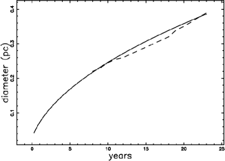
Figure 1: Diameter as a function of time for a self-gravitating medium (full line) when $\theta=0.001$ (equatorial plane) and astronomical data of torus only as extracted from Figure 3 in [14] (dashed line) . Physical parameters as in Table 1.

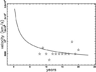
Figure 2: Velocity as a function of time for a self-gravitating medium (full line) when $\theta=0.001$ (equatorial plane) and astronomical data of torus only as extracted from Figure 3 in [14] (empty stars). Physical parameters as in Table 1.

Fig. 3 reports the asymmetric expansion in a section crossing the center, Figures 4 and 5 report the radius and the velocity respectively as a function of the position angle $\theta$.

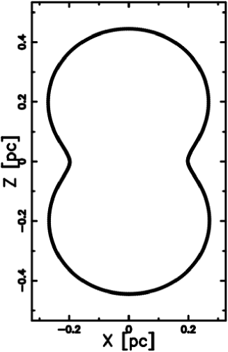
Figure 3: Section of SN  1987A  in the x-z plane. The horizontal and vertical axis are in $pc$. Physical parameters as in Table 1.

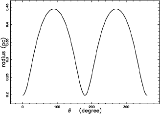
Figure 4: Radius in $pc$ of SN  1987A  as a function of the position angle in degrees for a self-gravitating medium. Physical parameters as in Table 1.

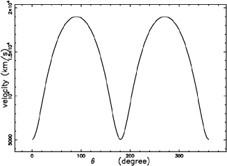
Figure 5: Velocity in $\frac{km}{s}$ of SN  1987A  as a function of the position angle in degrees for a self-gravitating medium. Physical parameters as in Table 1.

The swept mass in our model is not constant but varies with the value of latitude , see Figure 6.

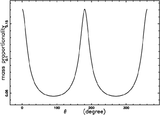
Figure 6: Swept mass of SN  1987A  in arbitrary units as a function of the position angle in degrees , for a self-gravitating medium. Physical parameters as in Table 1.

4.2 The image

We assume that the emissivity is proportional to the number density.

$$j_{\nu}\zeta=KC(s)\quad,$$ (23)

where $j_{\nu}$ is the emission coefficient and $K$ is a constant function. This can be the case of synchrotron radiation in presence of an isotropic distribution of electrons with a power law distribution in energy, $N(E)$,

$$N(E)dE=K_{s}E^{-\gamma_{f}}\quad,$$ (24)

where $K_{s}$ is a constant. The source of synchrotron luminosity is assumed here to be the flux of kinetic energy, $L_{m}$,

$$L_{m}=\frac{1}{2}\rho AV^{3}\quad,$$ (25)

where $A$ is the considered area, see formula (A28) in [15]. In our case $A=4\pi R^{2}$, which means

$$L_{m}=\frac{1}{2}\rho 4\pi R^{2}V^{3}\quad,$$ (26)

where $R$ is the instantaneous radius of the SNR and $\rho$ is the density in the advancing layer in which the synchrotron emission takes place. The total observed luminosity can be expressed as

$$L_{tot}=\epsilon L_{m}\quad,$$ (27)

where $\epsilon$ is a constant of conversion from the mechanical luminosity to the total observed luminosity in synchrotron emission.

The numerical algorithm which allows us to build a complex image is now outlined.

• An empty (value=0) memory grid ${\mathcal{M}}(i,j,k)$ which contains $NDIM^{3}$ pixels is considered

• We first generate an internal 3D surface by rotating the ideal image $180^{\circ}$ around the polar direction and a second external surface at a fixed distance $\Delta R$ from the first surface. As an example, we fixed $\Delta R=R/12$, where $R$ is the momentary radius of expansion. The points on the memory grid which lie between the internal and external surfaces are memorized on ${\mathcal{M}}(i,j,k)$ with a variable integer number according to formula (26) and density $\rho$ proportional to the swept mass, see Fig. 6.

• Each point of ${\mathcal{M}}(i,j,k)$ has spatial coordinates $x,y,z$ which can be represented by the following $1\times 3$ matrix, $A$,

  $$A=\left[\begin{array}[]{c}x\\ \vskip 6.0pt plus 2.0pt minus 2.0pt\cr y\\ \vskip 6.0pt plus 2.0pt minus 2.0pt\cr{\it z}\end{array}\right]\quad.$$ (28)

  The orientation of the object is characterized by the Euler angles $(\Phi,\Theta,\Psi)$ and therefore by a total $3\times 3$ rotation matrix, $E$, see [16]. The matrix point is represented by the following $1\times 3$ matrix, $B$,

  $$B=E\cdot A\quad.$$ (29)

• The intensity map is obtained by summing the points of the rotated images along a particular direction.

• The effect of the insertion of a threshold intensity , $I_{tr}$ , given by the observational techniques , is now analyzed. The threshold intensity can be parametrized to $I_{max}$, the maximum value of intensity characterizing the map.

The image of SN  1987A  having polar axis along the z-direction, is shown in Fig. 7. The image for a realistically rotated SN  1987A  is shown in Fig. 8 and a comparison should be done with the observed triple ring system as reported in Figure 1 of [5] where the outer lobes are explained by light-echo effects.

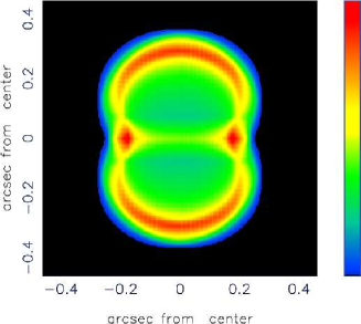
Figure 7: Map of the theoretical intensity of SN  1987A  in the presence of a self-gravitating medium.. Physical parameters as in Table 1. The three Euler angles characterizing the orientation are $\Phi$=180^∘, $\Theta$=90 ^∘ and $\Psi$=0 ^∘. This combination of Euler angles corresponds to the rotated image with the polar axis along the z-axis.

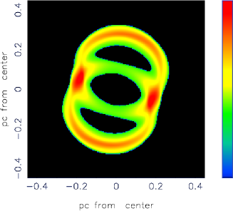
Figure 8: Model map of SN  1987A  rotated in accordance with the observations, for a self-gravitating medium. Physical parameters as in Table 1. the orientation of the observer are $\Phi$=105^∘, $\Theta$=55 ^∘ and $\Psi$=-165 ^∘. This combination of Euler angles corresponds to the observed image. In this map $I_{tr}=I_{max}/4$

Two cuts of intensity are reported in Figure 9, and is interesting to note that the polar cut is characterized by four spikes.

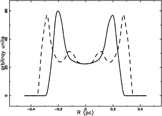
Figure 9: Two cuts of the model intensity across the center of the realistically rotated SN  1987A  : equatorial cut (full line) and polar cut (dotted line).

Here conversely the two outer lobes are explained by the image theory applied to a thin advancing shell.

5 Conclusions

Law of motion The presence of a thin self-gravitating disk of gas which is characterized by a Maxwellian distribution in velocity and distribution of density which varies only in the z-direction produces an axial symmetry in the temporal evolution of a SN. The resulting Eq. (22) has a form which can be solved numerically. The results depend from the chosen latitude and more precisely the radius as function of the time is maximum at the poles and minimum at the equator. A comparison between the observed radius and the velocity at the equator, see [14], gives an agreement of $92\%$ for the theoretical versus observed radius and of $62\%$ for the theoretical versus observed velocity. This is the first result that confirms the rationality of the method here presented. The momentum carried away by the photons can be modeled by introducing a reasonable form for the photon’s losses , see eqn. ( 20).

Images

The combination of different processes such as the bipolar 3D shape , the thin layer approximation (which means advancing layer having thickness $\approx 1/10$ of the momentary radius), the conversion of the rate of kinetic energy into luminosity and the observer’s point of view allows to simulate the observed triple ring morphology of SN  1987A  . The framework here adopted is similar to that adopted to explain the asymmetric shape of the nebula around $\eta$-Carinae (Homunculus), see [17, 18]. We therefore suggest that the astronomers should map the non rotated radius and velocity of SN  1987A  following the outlines of Table 1 in [19]. These maps , if realized , will produce a more clear framework for the observed triple ring. The suggested similarity of the triple ring system of SN  1987A  with $\eta$-Carinae is the second result which ensures the rationality of the method here presented.

REFERENCES

REFERENCES

- [1] Chevalier R A 1982 Self-similar solutions for the interaction of stellar ejecta with an external medium ApJ 258, 790
- [2] Chevalier R A 1982 The radio and X-ray emission from type II supernovae ApJ 259, 302
- [3] Reynolds S P and Gilmore D M 1986 Radio observations of the remnant of the supernova of A.D. 1006. I - Total intensity observations AJ 92, 1138
- [4] Morris T and Podsiadlowski P 2007 The Triple-Ring Nebula Around SN 1987A: Fingerprint of a Binary Merger Science 315, 1103 (Preprint arXiv:astro-ph/0703317)
- [5] Tziamtzis A, Lundqvist P, Gröningsson P and Nasoudi-Shoar S 2011 The outer rings of SN 1987A A&A 527 A35 (Preprint 1008.3387)
- [6] Zaninetti L 2012 On the spherical-axial transition in supernova remnants Astrophysics and Space Science 337, 581 (Preprint 1109.4012)
- [7] Bertin G 2000 Dynamics of Galaxies (Cambridge: Cambridge University Press.)
- [8] Padmanabhan P 2002 Theoretical astrophysics. Vol. III: Galaxies and Cosmology (Cambridge, MA: Cambridge University Press)
- [9] Hill C J 1828 Ueber die Integration logarithmisch-rationaler Differentiale. J. Reine Angew. Math. 3, 101
- [10] Lewin L 1981 Polylogarithms and associated functions. (New York: North Holland)
- [11] Olver F W J e, Lozier D W e, Boisvert R F e and Clark C W e 2010 NIST handbook of mathematical functions. (Cambridge: Cambridge University Press. )
- [12] Press W H, Teukolsky S A, Vetterling W T and Flannery B P 1992 Numerical Recipes in FORTRAN. The Art of Scientific Computing (Cambridge: Cambridge University Press)
- [13] Racusin J L, Park S, Zhekov S, Burrows D N, Garmire G P and McCray R 2009 X-ray Evolution of SNR 1987A: The Radial Expansion ApJ 703, 1752 (Preprint 0908.2097)
- [14] Chiad B T, Karim L M and Ali L T 2012 Study the Radial Expansion of SN 1987A Using Counting Pixels Method International Journal of Astronomy and Astrophysics 2, 199
- [15] De Young D S 2002 The physics of extragalactic radio sources (Chicago: University of Chicago Press)
- [16] Goldstein H, Poole C and Safko J 2002 Classical mechanics (San Francisco: Addison-Wesley)
- [17] Zaninetti L 2010 On the 3D structure of the nebula around -Carinae Advances in Space Research 46, 1341 (Preprint 1010.2364)
- [18] Zaninetti L 2012 Interaction of planetary nebulae , Eta-Carinae and supernova remnants with the Interstellar Medium, In Interstellar Medium: New Research , Cancellieri B. and Mamedov V Eds. (NY: Nova Publishers) pp 91–146
- [19] Smith N 2006 The Structure of the Homunculus. I. Shape and Latitude Dependence from H2 and Fe II Velocity Maps of eta Carinae ApJ 644, 1151 (Preprint arXiv:astro-ph/0602464)