Effect of Coordination Number on Nonequilibrium Critical Point

Abstract

We study the nonequilibrium critical point of the zero-temperature random-field Ising model on a triangular lattice and compare it with known results on honeycomb, square, and simple cubic lattices. We suggest that the coordination number of the lattice rather than its dimension plays the key role in determining the universality class of the nonequilibrium critical behavior. This is discussed in the context of numerical evidence that equilibrium and nonequilibrium critical points of the zero-temperature random-field Ising model belong to the same universality class. The physics of this curious result is not fully understood.

I Introduction

Systems with quenched disorder tend to respond to a smoothly varying force by way of avalanches in their structure  sethna1 ; bertotti ; durin ; fisher1 ; miguel . Generally, the avalanches are microscopic and therefore the response is macroscopically smooth. However, there are several instances in nature where the response exhibits an abrupt and catastrophic jump discontinuity: snow falls gently on a mountain for days before tons of snow may move abruptly in an avalanche. This cannot be attributed to the last snowflake before the avalanche. Similarly, landslides may occur abruptly during periods of incessant rain. Earthquakes are sporadic and sudden effects of the tectonic plates pressing against each other all the time. A more familiar and repeatable example from a physics laboratory is the Barkhausen noise on magnetization curves stoner . The theory of the Barkhausen noise has been studied extensively in the framework of the zero-temperature nonequilibrium random-field Ising model of a ferromagnet on a lattice sethna2 . The disorder is normally modeled by an on-site Gaussian random-field with average value zero and standard deviation $\sigma$. Numerical simulations on $d$-dimensional lattices ($d>1$) reveal that there is a critical value $\sigma_{c}$ such that for $\sigma>\sigma_{c}$, the response of the system, i.e., the magnetization $m(h,\sigma)$ in an applied field $h$, is macroscopically smooth over the entire range of the applied field $-\infty<h<\infty$. For $\sigma<\sigma_{c}$, $m(h,\sigma)$ has a jump discontinuity at $h=h_{c}(\sigma)$. The size of the jump as well as $|h_{c}(\sigma)|$ decreases as $\sigma\rightarrow\sigma_{c}$. The point $\{\sigma_{c},h_{c}(\sigma_{c})\}$ is a nonequilibrium critical point exhibiting anomalous scale-invariant fluctuations and universality reminiscent of the equilibrium critical point phenomena.

The similarity between the nonequilibrium and equilibrium critical behavior has a reason, but one that is not fully understood. The equilibrium critical point in a system with quenched disorder is controlled by a stable zero-temperature fixed point fisher2 . Therefore, it is not entirely surprising to observe critical behavior at zero temperature by varying the parameter $\sigma$. Let us consider zero-temperature equilibrium magnetization curves for different values of $\sigma$. We may expect smooth trajectories for $\sigma>\sigma_{c}$, jump discontinuities for $\sigma<\sigma_{c}$, and a vanishing jump discontinuity at $\sigma=\sigma_{c}$ just as in the case of the nonequilibrium magnetization curves. The only difference will be that the equilibrium case would show no hysteresis and therefore all singularities will occur at $h=0$. The nonequilibrium response will show hysteresis and the singularities for $\sigma\leq\sigma_{c}$ will occur on the lower and upper halves of the hysteresis loop in a symmetrical fashion. One may ask if the noise on the equilibrium magnetization curves and the anomalous fluctuations at the equilibrium critical points have the same character as their nonequilibrium counterparts. Surprisingly, the answer to this question is that they do in the framework of the zero-temperature random-field Ising model. Numerical studies of the model provide strong evidence that the disorder-induced critical points in equilibrium as well as the nonequilibrium case belong to the same universality class liu . This serendipity may provide a way to infer nonequilibrium properties of a system from its equilibrium properties. It is intriguing. As a system is driven by an applied field from $h=-\infty$ to $\infty$, the nonequilibrium trajectory of the system comprises a sequence of metastable states. The equilibrium trajectory goes through the states of global minima of the energy. What is the physics that puts the two cases in the same universality class?

We focus on a similar but smaller question. It is known that the universality class of an equilibrium critical point is determined by the dimensionality of the lattice and not by the kind of Bravais lattice it is. The reason for this is well understood. The correlation length diverges at the critical point and therefore the short-range structure of the lattice is irrelevant to the critical behavior. In contrast, the existence of a nonequilibrium critical point, let alone its universality class, appears to be determined by the coordination number of the lattice rather than its dimensionality. An exact calculation on the Bethe lattice of an arbitrary coordination number $z$ shows that a nonequilibrium critical point exists only if $z>3$  dhar . Numerical simulations suggest that the significance of this result goes beyond the Bethe lattice; periodic lattices with $z=3$ in $d=2,3$ do not possess a nonequilibrium critical point  sabhapandit . Although these results have been reported quite some time ago, their significance does not appear to be widely recognized. For example, numerical simulations have often failed to settle the question if there is a nonequilibrium critical point on the square lattice ($z=4$) bertotti . Recent results indicate that it is there spasojevic . This has been taken to indicate that the lower critical dimension for nonequilibrium critical behavior is equal to 2. However, it has been shown earlier that there is no nonequilibrium phase transition on a honeycomb lattice sabhapandit . Indeed, there is good evidence that the nonequilibrium critical behavior is controlled by a lower critical coordination number ($z=4$) rather than a lower critical dimension ($d=2$).

In this paper we study the nonequilibrium critical point on a triangular lattice ($z=6$) reiterating the importance of the coordination number rather than the dimensionality of the lattice. We show the existence of a critical point and estimate the critical exponent $\nu$. Within numerical errors we find $\nu$ to be tantalizingly close to the value reported for the simple cubic lattice. The simple cubic and the triangular lattices have the same coordination number ($z=6$) and it is possible that the values of the nonequilibrium critical exponents depend on $z$ just as their existence depends on $z$. Indeed, it may be useful to study the triangular lattice with gradual dilution of one of the three sublattices comprising it. This way, one can go continuously from a triangular ($z=6$) to a honeycomb $(z=3)$ lattice and study the effect of $z$ on the critical behavior. However, this is beyond the scope of the present paper.

II The Model and Simulations on a Triangular Lattice

The random-field Ising model is characterized by the Hamiltonian,

$$H=-J\sum_{i,j}s_{i}s_{j}-\sum_{i}h_{i}s_{i}-h\sum_{i}s_{i},$$ (1)

where $\{s_{i}=\pm 1\}$ are Ising spins on a triangular lattice and $\{h_{i}\}$ are identically distributed independent random fields drawn from a Gaussian distribution with mean zero and standard deviation $\sigma$. Periodic boundary conditions are imposed. Here $J$ is the ferromagnetic interaction between nearest neighbors and $h$ is an external field that is varied adiabatically from $-\infty$ to $\infty$. A stable state of the system at $h$ has each spin aligned along the net field at its site. As $h$ is ramped up, numerous instabilities occur where a spin flips up and causes neighboring spins to flip up in an avalanche. When this happens, $h$ is kept constant during the avalanche and then increased again until the next avalanche. The curve $m(h,\sigma)$ is the locus of the magnetization of locally stable states along increasing $h$ for a random-field distribution characterized by standard deviation $\sigma$.

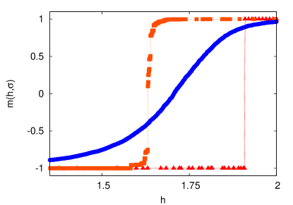
In contrast to the case of the square lattice spasojevic , it takes a rather modest effort to see that the curve $m(h,\sigma)$ makes a transition between a discontinuous and a continuous form as $\sigma$ is increased. Fig. 1 shows $m(h,\sigma)$ in increasing $h$ for $\sigma$=1 (red triangles), $\sigma$=1.275 (orange squares), and $\sigma$=2 (blue continuous line) on a $1000\times 1000$ triangular lattice. Only the data in the range $1.3\leq h\leq 2$ are shown. The curve for $\sigma=1$ shows a jump in the magnetization at $h\approx 1.9$, but the curve for $\sigma=2$ is smooth. This suggests that a transition occurs at a critical value $\sigma_{c}$ ($1<\sigma_{c}<2$) as $\sigma$ is increased. However, it is difficult to locate the exact $\sigma_{c}$. The difficulty is illustrated by the $m(h,\sigma)$ curve for $\sigma=1.275$, which is close to the critical value $\sigma_{c}$. Ideally, we would like to see a single jump in an otherwise smooth curve, and the size of the jump approaching zero as $\sigma\rightarrow\sigma_{c}$ from below. However, the critical point $\{\sigma_{c},h_{c}\}$ is characterized by anomalously large fluctuations. Therefore, the critical curve in a typical simulation is punctuated by several jumps of different sizes. Increasing the system size does not alleviate this difficulty because the critical fluctuations also increase in proportion. We will return to this point in the following paragraph. For now we note another point of caution even in the case $\sigma<<\sigma_{c}$ where a large jump in $m(h,\sigma)$ is rather obvious. In the limit $\sigma\rightarrow 0$, the initial state of the system ($h=-\infty$, all spins down) has an instability such that the first spin to flip up in increasing $h$ causes all the spins in the system to flip up. This is easily understood. The first spin flips up at $h=6J-h_{max}$, where $h_{max}$ is the maximum random field on an $L\times L$ lattice, $h_{max}^{2}\approx\sigma^{2}\ln{2\pi\sigma^{2}/L^{4}}$. After the first spin flips up, the effective field on its neighbors becomes $4J-h_{i}$, which is positive with probability unity in the limit $\sigma\rightarrow 0$, and so all the neighbors flip up. Indeed, this causes an infinite avalanche leading to a state with all spins up. It is important to distinguish this instability from a genuine disorder-driven discontinuity that may occur for larger values of $\sigma$ sabhapandit .

It is relatively easy to spot a large first-order discontinuity in the magnetization curve $m(h,\sigma)$. However, it is not as straightforward as it may look at first sight. In simulations as well as in experiments, it is difficult to distinguish between a truly discontinuous curve and one that may be smooth but steeply rising. We have to employ a method that takes into account the nature of fluctuations underlying the phase transition. One of the methods used in the literature is that of the Binder cumulant binder calculated from the averages of the square and the fourth power of the magnetization. It has been used for estimating the critical temperature of Ising models and distinguishing between first-order and second-order phase transitions in models without quenched disorder and applied field. For the present problem, we use a method that counts all the avalanches of size $s$ as the system is driven from $h=-\infty$ to $\infty$. Let $P(s,\sigma)$ be the probability of an avalanche of size $s$, where $\sigma$ is the standard deviation of the random-field distribution. In general, $P(s,\sigma)$ is a product of an algebraically decreasing part and an exponentially decreasing part with a cutoff $s_{0}$ that sets the scale of the avalanches. At a critical point we have $s_{0}=\infty$ and therefore the avalanches become scale invariant.

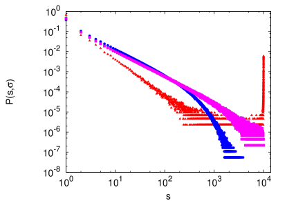
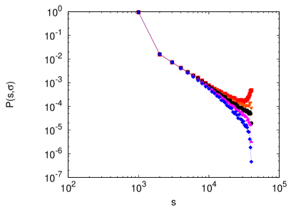
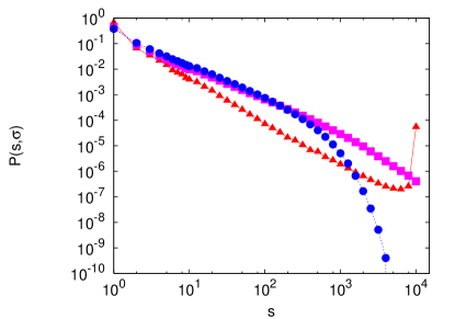
The distribution $P(s,\sigma)$ has a different form depending upon whether $m(h,\sigma)$ is continuous or discontinuous  farrow . The idea is illustrated by Fig. 2, which shows the probability $P(s,\sigma)$ of an avalanche of size $s$ for $\sigma$=1.25 (red triangles), 1.63 (pink squares), and 2 (blue), respectively. The $m(h,\sigma)$ curve for $\sigma=1.25$ has a jump discontinuity. The avalanches near the discontinuity are very large and may span the entire system. Away from the discontinuity the avalanches are small and $P(s,\sigma)$ decreases exponentially with $s$. Thus the defining trend of the avalanche distribution (red triangles) along a discontinuous magnetization curve is an algebraically decreasing $P(s,\sigma)$ followed by a peak at $s\approx L\times L$. In contrast to this, the avalanches along a noncritical continuous magnetization curve, e.g., the $m(h,\sigma)$ curve for $\sigma=2$ in Fig. 1, are exponentially small with a cutoff much smaller than $L\times L$. This is reflected in the corresponding curve (blue circles) in Fig. 2 by an initial algebraic decrease of $P(s,\sigma)$ followed by a more rapid decrease characteristic of the cutoff. Thus the distribution of avalanche sizes along the magnetization curve provides us with a method to distinguish between a smooth $m(h,\sigma)$ and one with a discontinuity. However, our goal is to identify a critical $m(h,\sigma)$ curve where the discontinuity just vanishes, i.e., to determine $\sigma_{c}$. This is evidently a difficult task. At $\sigma_{c}$, we may expect $\ln{P(s,\sigma)}$ to vary linearly with $\ln{s}$ in the entire range $1<s<L\times L$ with the peak at $s\approx L\times L$ just vanishing. It is difficult to implement this criterion strictly within a reasonable computational effort because avalanche distributions for different $\sigma$ have to be obtained and compared with each other. We have tried to meet this criterion within a reasonable error to the second decimal place in $\sigma_{c}$ as illustrated by the pink (squares) curve in Fig. 2 for $\sigma=1.63$; $\sigma_{c}=1.63\pm 0.01$ is our best estimate for the critical point on the $100\times 100$ triangular lattice. This estimate has been obtained from 50000 independent realizations of the random-field distribution and took nearly a day of CPU time on our computer. We have often used binned data along with the unbinned data to find the best estimate for $\sigma_{c}$. As an illustration, Fig. 3 shows the binned data for avalanches on a $200\times 200$ lattice. The possible range of an avalanche lies between a single spin flip and $4\times 10^{4}$ spin flips. This range is divided into 40 linear bins and the weight of each bin is represented by a point on the curve. See the caption on Fig. 3 for more details. We have also analyzed the data shown in Fig. 2 using logarithmic binning. The result is shown in Figure (4). As may be expected, the fat tails of the distributions shown in Fig. 2 are replaced by more clearly defined curves.

III Finite Size Effects

Following the procedure outlined above, we have determined $\sigma_{c}(L)$ for lattices of linear size $L=100-400$. The results are presented in Table I.

Table 1: $\sigma_{c}(L)$ for lattices of linear size $L=100-400$.

$L$	$\sigma_{c}$(L)
100	1.63 $\pm$ 0.01
125	1.58 $\pm$ 0.01
150	1.545 $\pm$ 0.005
175	1.52 $\pm$ 0.01
200	1.50 $\pm$ 0.01
250	1.47 $\pm$ 0.01
300	1.45 $\pm$ 0.01
400	1.42 $\pm$ 0.01

As $\sigma\rightarrow\sigma_{c}$ from below, the size of the avalanche diverges with the exponent $\nu$, i.e., $s\sim(\sigma-\sigma_{c})^{-\nu}$. On a finite lattice, the largest avalanche is limited by the size of the lattice. Thus we define a lattice-dependent critical value $\sigma_{c}(L)$ by the equation

$$L^{-\frac{1}{\nu}}=\frac{\sigma_{c}(L)-\sigma_{c}}{\sigma_{c}}\mbox{ or }-\frac{1}{\nu}\log_{10}L=\log_{10}\left[\frac{\sigma_{c}(L)}{\sigma_{c}}-1\right]$$ (2)

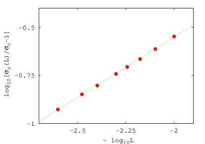
We determine $\sigma_{c}$ by requiring the data in Table I to fit a straight line. The best fit to the straight line is shown in Fig. 5. The slope of the line gives $1/\nu=0.62$, or $\nu=1.6\pm 0.2$. The data shown in Table I are based on linear binning. They change slightly if logarithmic binning is used; we get $\sigma_{c}(L)=1.525\pm 0.005$ for $L=175$, $\sigma_{c}(L)=1.41\pm 0.01$ for $L=400$, and estimates of $\sigma_{c}(L)$ for other values of $L$ remain unchanged. The quality of the best straight line fit to the changed data is slightly poorer as compared to the one shown in Fig. 5, but it yields $\nu=1.5\pm 0.2$.

Although it is a good practice to fit the data with a minimum number of adjustable parameters, we also tried the following form with an additional parameter $a$:

$$L^{-\frac{1}{\nu}}=\frac{\sigma_{c}(L)-\sigma_{c}^{\prime}}{a}$$ (3)

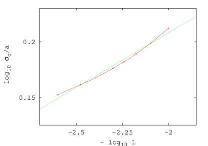
We find that the best straight line fit to Eq. (3) is obtained when $\sigma_{c}^{\prime}=\sigma_{c}$ obtained from fitting the data to Eq. (2). If we set $\sigma_{c}^{\prime}=0$, we are not able to fit the data to a straight line. This shows that we must have $\sigma_{c}^{\prime}>0$. Figure 6 shows the data and the nearest straight line fit to it for $\sigma_{c}^{\prime}=0$ and $a=1$. The slope of the straight line corresponds to $\nu=10.2$ approximately. The role of the parameter $a$ is only to shift the curve along the $y$ axis. It does not affect the slope of the straight line that best fits the data.

The existence of a critical point is expected to be accompanied by scaling of thermodynamic functions in its vicinity. Thus the existence of a critical value $\sigma_{c}>0$ means that a quantity such as $P(s,\sigma)$, which is in general a function of two independent variables $s$ and $\sigma$, must become a function of a single variable, say, $s|\frac{\sigma_{c}-\sigma}{\sigma}|^{p}$ as $\sigma\rightarrow\sigma_{c}$ for some value of the exponent $p$. Let us define

$$r=\frac{\sigma_{c}(L)-\sigma}{\sigma}.$$ (4)

The scaling hypothesis requires that as $\sigma\rightarrow\sigma_{c}(L)$, the plots of $s^{q}P(s,\sigma)$ vs $s|r|^{p}$ for a fixed lattice of size $L\times L$ and different values of $\sigma$ should collapse on a single curve for suitable choices of the exponents $p$ and $q$. Figure 7 shows such a collapse for a $200\times 200$ lattice. The collapsed curves are distinct for $r<0$ ($q=2$ and $p=0.66$) and $r>0$ ($q=2$ and $p=0.25$). The exponents $p$ and $q$ may be related to standard critical point exponents, e.g., $q=\tau+\sigma\beta\delta$  spasojevic ; perkovic2 . The family of collapsed curves for different thermodynamic functions can be used to determine standard critical exponents, but in the present case we do not have sufficient data to take this approach. We are content to note that the avalanche size distributions show a reasonable collapse in a rather wide region around the critical point.

IV Discussion

We have shown that there is a critical point in the behavior of the zero-temperature random-field Ising model on a triangular lattice. This result assumes significance in the context of a long-standing speculation as to whether there is a nonequilibrium critical point in two dimensions. Generally, the hysteretic behavior of the random-field Ising model on a square lattice has been taken to characterize the behavior of the model in two dimensions. However, the coordination number $z$ of the lattice seems to be a key parameter. Two-dimensional lattices with $z=3$ (honeycomb structure) do not have a critical point sabhapandit . Studies on a square lattice ($z=4$), were initially inconclusive but more recent studies suggest that it has a critical point spasojevic . The existence of a critical point on a triangular lattice ($z=6$) can be verified with a rather modest effort as shown here. These results suggest that a lower critical coordination number has a greater significance for determining critical avalanches than a lower critical dimension. Although this goes against the spirit of the renormalization group theory that the short-range structure of the lattice should become irrelevant at the divergence of the correlation length, some reflection shows that it is reasonable in the context of avalanches. It is reasonable that the coordination number of the lattice should determine how far an avalanche can propagate from its point of origin. Therefore, a minimum coordination number must be necessary for the divergence of avalanches irrespective of the dimensionality of the lattice.

If the existence of the nonequilibrium critical point depends on a lower critical coordination number rather than a lower critical dimension of the lattice, then it is natural to ask if the critical exponents depend upon $z$ as well. An exact solution of the random-field Ising model on a Bethe lattice of coordination number $z$ shows that the exponents are independent of $z$ as long as $z\geq 4$. Numerical results on periodic lattices do not give such a clear indication. Let us focus on the critical exponent $\nu$. The uncertainty in the numerical determination of this exponent is rather large, although it is of central importance conceptually. The best estimates are $\nu=5.15\pm 0.20$ on a square ($z=4$) lattice spasojevic , $\nu=1.4\pm 0.2$ on a simple cubic ($z=6$) lattice perkovic , and the present result $\nu=1.6\pm 0.2$ on a triangular ($z=6$) lattice. The closeness of $\nu$ on simple cubic and triangular lattice is interesting in view of the fact that the coordination number of both lattices is the same.

Figure 1: (Color online) Magnetization curves in increasing field $h$ for $\sigma=1$ (red discontinuous curve comprising triangles), $\sigma=2$ (blue continuous curve), and at an intermediate value $\sigma=1.275$ (orange squares with several jumps).

Figure 2: (Color online) Plot of $P(s,\sigma)$, the probability of an avalanche of size $s$ on a $100\times 100$ triangular lattice for $\sigma=1.25$ (red triangles, lower curve with a peak at $s\approx 10^{4}$), $\sigma=1.63$ (pink squares, curve with its tail nearest to the red triangles peak), and $\sigma=2$ (blue circles, curve with is tail farthest from the red/triangles’ peak).

Figure 3: (Color online) Binned data for $P(s,\sigma)$ vs $s$ on a $200\times 200$ triangular lattice for $\sigma=1.45$ (red squares), 1.48 (orange inverted triangles), 1.50 (black circles), 1.52 (pink triangles), and 1.54 (blue diamonds). Generally, the last point in each curve may be ignored because of less data in the last bin. We estimate $\sigma_{c}=1.50$ for a lattice of linear size $L=200$ because the corresponding distribution is nearly linear over the entire range of avalanche sizes. Avalanches for $\sigma<\sigma_{c}$ tend to show a $\delta$-function peak at the largest avalanche, while avalanches for $\sigma>\sigma_{c}$ tend to bend down. The opposite trends for $\sigma<\sigma_{c}$ and $\sigma>\sigma_{c}$ become more pronounced as one moves farther away from $\sigma_{c}$.

Figure 4: (Color online) Plot of $P(s,\sigma)$ using the same data as in Fig. 2 but using logarithmic binning. The colors and symbols have the same meaning as in Fig. 2.

Figure 5: (Color online) Finite-size scaling: plot of - $\log_{10}L$ ($x$ axis) vs $\log_{10}[\sigma_{c}(L)$/$\sigma_{c}$-1] ($y$ axis). The parameter $\sigma_{c}=1.27$ is determined by the best linear fit to the data of Table I. The slope of the line yields $\nu=1.6$.

Figure 6: (Color online) Plot of - $\log_{10}L$ ($x$ axis) vs $\log_{10}\sigma_{c}(L)/a$ for $a=1$ ($y$ axis). The curve does not fit well to a straight line. The straight line with a slope of 0.098 ($\nu=10.17$) shown in the figure is the best fit to the data. Changing the parameter $a$ shifts the curve along the $y$ axis.

Figure 7: (Color online) Data collapse: plot of $s^{q}P(s,\sigma)$ vs $s|r|^{p}$ for a $200\times 200$ lattice. The upper set of curves are for $\sigma=1.52,1.53,1.54,1.56$ ($\sigma>\sigma_{c}=1.50$). These collapse reasonably on top of each other for $q=2$ and $p=0.66$. The lower set of curves are for $\sigma=1.48,1.47,1.46,1.45$ ($\sigma<\sigma_{c}$). These too show reasonable collapse for $q=2$ and $p=0.25$.

References

- (1) J. P. Sethna, K. A. Dahmen, and C. R. Myers, Nature (London) 410, 242 (2001).
- (2) The Science of Hysteresis, edited by G. Bertotti and I. Mayergoyz (Academic, New York, 2005).
- (3) G. Durin and S. Zapperi, in bertotti .
- (4) D. S. Fisher, Phys. Rep. 301, 113 (1998).
- (5) M. C. Miguel, A. Vespignani, S. Zapperi, J. Weiss, and J. R. Grosso, Nature (London) 410, 667 (2001).
- (6) See, for example, E. C. Stoner, Rev. Mod. Phys. 25, 2 (1953); the main features of Barkhausen noise discovered in these early experiments are still topics of current research.
- (7) J. P. Sethna, K. A. Dahmen, and O. Percovic, in bertotti and references therein.
- (8) D. S. Fisher, Phys. Rev. Lett 56, 416 (1986).
- (9) Y. Liu and K. A. Dahmen, Phys. Rev. E 79, 061124 (2009).
- (10) D. Dhar, P. Shukla, and J. P. Sethna, J. Phys. A 30, 5259 (1997).
- (11) S. Sabhapandit, D. Dhar, and P. Shukla, Phys. Rev. Lett. 88, 197202 (2002).
- (12) D. Spasojevic, S. Janicevic, and M. Knezevic, Phys. Rev. Lett. 106, 175701 (2011); Phys. Rev. E 84, 051119 (2011).
- (13) K. Binder, Phys. Rev. Lett. 47, 693 (1981); Z. Phys. B 43, 119 (1981); K. Binder and H. J. Herrmann, in Monte Carlo Simulations in Statistical Physics edited by M. Cardona, P. Fulde, K. von Klitzing, and H. J. Queisser (Springer, Berlin, 1992).
- (14) C. L. Farrow, P. Shukla, and P. M. Duxbury, J. Phys. A: Math. Theor. 40, F581 (2007); P. Shukla, Pramana 71, 319 (2008).
- (15) O. Perkovic, K. A. Dahmen, and J. P. Sethna, arXiv:cond-mat/9609072v1.
- (16) O. Perkovic, K. A. Dahmen, and J. P. Sethna, Phys. Rev. B 59, 6106 (1999).