A Note on Graphs of Linear Rank-Width $1$

Abstract.

We prove that a connected graph has linear rank-width $1$ if and only if it is a distance-hereditary graph and its split decomposition tree is a path. An immediate consequence is that one can decide in linear time whether a graph has linear rank-width at most $1$, and give an obstruction if not. Other immediate consequences are several characterisations of graphs of linear rank-width $1$. In particular a connected graph has linear rank-width $1$ if and only if it is locally equivalent to a caterpillar if and only if it is a vertex-minor of a path [O-joung Kwon and Sang-il Oum, Graphs of small rank-width are pivot-minors of graphs of small tree-width, to appear in Discrete Applied Mathematics] if and only if it does not contain the co-$K_{2}$ graph, the Net graph and the $5$-cycle graph as vertex-minors [Isolde Adler, Arthur M. Farley and Andrzej Proskurowski, Obstructions for linear rank-width at most $1$, to appear in Discrete Applied Mathematics].

1. Introduction

In their investigations for the recognition of graphs of bounded clique-width [8] Oum and Seymour introduced the notion of rank-width [20] of a graph. Rank-width appeared to have several nice combinatorial properties, in particular it is related to the vertex-minor inclusion, and have proven the last years its importance in studying the structure of graphs of bounded clique-width [19, 20, 9, 15]. Linear rank-width is related to rank-width in the same way path-width [22] is related to tree-width [23]. Indeed, linear rank-width is the linearised version of rank-width and studying graphs of bounded linear rank-width is a first step in studying the structure of graphs of bounded rank-width which is not yet well understood. Not much is known about linear rank-width. The computation of the linear rank-width of forests is investigated in [2] and it is proved in [16] that graphs of linear rank-width $k$ are vertex-minors of graphs of path-width at most $k+1$. Ganian defined in [14] the notion of thread graphs and proved that they correspond exactly to graphs of linear rank-width $1$ and authors of [1] used it to exhibit the set of vertex-minor obstructions for linear rank-width $1$. In this paper we investigate in a different way the structure of graphs of linear rank-width $1$.

Distance hereditary graphs [3] are a well-known and well-studied class of graphs because of their multiple nice algorithmic properties. They admit several characterisations, in particular they correspond exactly to graphs of rank-width at most $1$ [19] and are the graphs that are totally decomposable with respect to split decomposition [10]. Split decomposition is a graph decomposition introduced by Cunningham and Edmonds and has proved its importance in algorithmic and structural graph theory (see for instance [4, 5, 6, 7, 21] to cite a few). We give in this paper the following characterisation of graphs of linear rank-width $1$ which implies all the known characterisations of graphs of linear rank-width $1$.

Theorem 1.

A connected graph $G$ has linear rank width $1$ if and only if it is a distance hereditary graph and its split decomposition tree is a path.

A first consequence of this theorem is that we can derive in a more direct way than in [1] the set of induced subgraph (or vertex-minor of pivot-minor) obstructions for linear rank-width $1$. Another consequence is a simple linear time algorithm for recognising graphs of linear rank-width $1$ (the only known one prior to this algorithm is the one that uses logical tools [9] and is not really practical). Our algorithm gives moreover an obstruction if it exists. Notice that a polynomial time algorithm for recognising graphs of linear rank-width $1$ is a consequence of the characterisation in terms of thread graphs given in [14].

The paper is organised as follows. Some definitions and notations are given in Section 2. In Section 3 we introduce the notion of split decomposition and prove our main theorem. We derive several characterisations and give a simple linear time algorithm (with a certificate) for the recognition of graphs of linear rank-width at most $1$.

2. Preliminaries

For two sets $A$ and $B$, we let $A\backslash B$ be the set $\{x\in A\mid x\notin B\}$. We often write $x$ to denote the set $\{x\}$. For sets $R$ and $C$, an $(R,C)$-matrix is a matrix where the rows are indexed by elements in $R$ and columns indexed by elements in $C$. For an $(R,C)$-matrix $M$, if $X\subseteq R$ and $Y\subseteq C$, we let ${M}[{X},{Y}]$ be the sub-matrix of $M$ the rows and the columns of which are indexed by $X$ and $Y$ respectively. We let $\operatorname{rk}$ be the matrix rank-function (the field will be clear from the context).

Our graph terminology is standard, see for instance [13]. A graph $G$ is a pair $(V(G),E(G))$ where $V(G)$ is the set of vertices and $E(G)$, the set of edges, is a set of unordered pairs of $V(G)$. An edge between $x$ and $y$ in a graph is denoted by $xy$ (equivalently $yx$). The subgraph of a graph $G$ induced by $X\subseteq V(G)$ is denoted by $G[X]$. Two graphs $G$ and $H$ are isomorphic if there exists a bijection $\varphi:V(G)\to V(H)$ such that $xy\in E(G)$ if and only if $\varphi(x)\varphi(y)\in E(H)$. All graphs are finite and loop-free.

A tree is an acyclic connected graph. In order to avoid confusions in some lemmas, we will call nodes the vertices of trees. The nodes of degree $1$ are called leaves. A path is a tree the vertices of which have all degree $2$, except two that have degree $1$. A caterpillar is a tree such that the removal of leaves results in a path.

A graph is distance hereditary if its induced subpaths are isometric [3]. Examples of distance hereditary graphs are trees, cliques, etc. There exist several characterisations of distance hereditary graphs. See for instance [17, Theorem 1] for a summary of some known characterisations of distance hereditary graphs.

The adjacency matrix of a graph $G$ is the $(V(G),V(G))$-matrix $A_{G}$ over $GF(2)$ where $A_{G}[x,y]=1$ if and only if $xy\in E(G)$. For a graph $G$, let $x_{1},\ldots,x_{n}$ be a linear ordering of its vertices. For each index $i$, we let $X_{i}:=\{x_{1},\ldots,x_{i}\}$ and $\overline{X_{i}}:=\{x_{i+1},\ldots,x_{n}\}$. The cutrank of the ordering $x_{1},\ldots,x_{n}$ is defined as

$$\operatorname{cutrk}_{G}(x_{1},\ldots,x_{n}) =\max\{\operatorname{rk}\left(A_{G}[X_{i},\overline{X_{i}}]\right)\mid 1\leq i\leq n\}.$$

The linear rank-width of a graph $G$ is defined as

$$\operatorname{lrw}(G) =\min\{\operatorname{cutrk}_{G}(x_{1},\ldots,x_{n})\mid x_{1},\ldots,x_{n}\ \textrm{is a linear ordering of $V(G)$}\}.$$

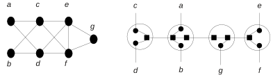
Figure 2. An example of a graph and its split decomposition tree.

The linear ordering $c,d,a,b,g,e,f$ of the graph in Figure 2 has cutrank $1$. It is worth noticing that if a graph $G$ is not connected and its connected components are $C_{1},\ldots,C_{t}$, then $\operatorname{lrw}(G)=\max\{\operatorname{lrw}(C_{i})\}_{1\leq i\leq t}$ since it suffices to concatenate in any order the linear ordering of optimal cutrank of its connected components.

For a graph $G$ and a vertex $x$ of $G$, the local complementation at $x$ consists in replacing the subgraph induced on the neighbours of $x$ by its complement. The resulting graph is denoted by $G*x$. A graph $H$ is locally equivalent to a graph $G$ if $H$ is obtained from $G$ by applying a sequence of local complementations, and $H$ is called a vertex-minor of $G$ if $H$ is isomorphic to an induced subgraph of a graph locally equivalent to $G$. The following relates vertex-minor and linear rank-width.

Proposition 1 ([19]).

Let $G$ and $H$ be two graphs. If $H$ is locally equivalent to $G$, then $\operatorname{lrw}(H)=\operatorname{lrw}(G)$. If $H$ is a vertex-minor of $G$, then $\operatorname{lrw}(H)\leq\operatorname{lrw}(G)$.

3. Linear rank-width $1$

We prove in this section our main theorem. Let us make precise some terminologies and notations.

3.1. Split decomposition

Two bipartitions $\{X_{1},X_{2}\}$ and $\{Y_{1},Y_{2}\}$ of a set $V$ overlap if $X_{i}\cap Y_{j}\neq\emptyset$ for all $i,j\in\{1,2\}$. A split in a connected graph $G$ is a bipartition $\{X,Y\}$ of the vertex set $V(G)$ such that $|X|,|Y|\geq 2$ and $\operatorname{rk}\left(A_{G}[X,Y]\right)=1$. A split $\{X,Y\}$ is strong if there is no other split $\{X^{\prime},Y^{\prime}\}$ such that $\{X,Y\}$ and $\{X^{\prime},Y^{\prime}\}$ overlap. Figure 1 shows a schematic view of splits. Notice that not all graphs have a split and those without a split are called prime. We follow [7] for the definition of a split decomposition tree.

Figure 1. Schematic view of splits.

If $\{X,Y\}$ is a split, then we let $G^{X}$ and $G^{Y}$ be the graphs with vertex set $X\cup\{h_{X}\}$ and $Y\cup\{h_{Y}\}$ respectively where the vertices $h_{X}$ and $h_{Y}$ are new and called neighbour markers of $G^{X}$ and $G^{Y}$ respectively, and with edge set

$$E(G^{X}) :=E(G[X])\cup\{xh_{X}\mid x\in X\ \textrm{and}\ N_{G}(x)\cap Y\neq\emptyset\},\qquad\textrm{and}$$

$$E(G^{Y}) :=E(G[Y])\cup\{yh_{Y}\mid y\in Y\ \textrm{and}\ N_{G}(y)\cap X\neq\emptyset\}.$$

A decomposition of a connected graph $G$ is defined inductively as follows: $\{G\}$ is the only decomposition of size $1$. If $\{G_{1},\ldots,G_{n}\}$ is a decomposition of size $n$ of $G$, then if $G_{i}$ has a split $\{X,Y\}$, then $\{G_{1},\ldots,G_{i-1},G^{X},G^{Y},G_{i+1},\ldots,G_{n}\}$ is a decomposition of size $n+1$. Notice that the decomposition process must terminate because the new graphs $G^{X}$ and $G^{Y}$ are smaller than $G_{i}$. The graphs $G_{i}$ of a decomposition are called blocks. If two blocks have neighbour markers, we call them neighbour blocks.

For every decomposition $\mathcal{D}$ of a connected graph $G$ we associate the graph $S(\mathcal{D})$ with vertex set $\bigcup_{G_{i}\in\mathcal{D}}V(G_{i})$ and edge set

$$\left(\bigcup_{G_{i}\in\mathcal{D}}E(G_{i})\right)\cup\{h_{X}h_{Y}\mid h_{X},h_{Y}\ \textrm{are neighbour markers}\}.$$

Edges in $E(S(\mathcal{D}))$ between neighbour markers of $\mathcal{D}$ are called marked edges and the others are called solid edges. One notices that subgraphs of $S(\mathcal{D})$ induced by solid edges are blocks of $\mathcal{D}$. Observe that each mark edge is an isthmus, and the marked edges form a matching.

Two decompositions $\mathcal{D}_{1}$ and $\mathcal{D}_{2}$ of a connected graph $G$ are isomorphic if there exists a graph isomorphism $f$ between $S(\mathcal{D}_{1})$ and $S(\mathcal{D}_{2})$ which preserves the marked edges, and such that $f(x)=x$ for all $x\in V(G)$. It is worth noticing that a graph can have several non isomorphic decompositions. However, a canonical decomposition can be defined. A decomposition is canonical if and only if: (i) each block is either prime (called prime block), or is isomorphic to a clique of size at least $3$ (called clique block) or to a star of size at least $3$ (called star block), (ii) no two clique blocks are neighbour, and (iii) if two star blocks are neighbour, then either their markers are both centres or both not centres. The following theorem is due to Cunningham and Edmonds [10], and Dahlhaus [11].

Theorem 2 ([10, 11]).

Every connected graph has a unique canonical decomposition, up to isomorphism. It can be obtained by iterated splitting relative to strong splits. This canonical decomposition can be computed in time $O(n+m)$ for every graph $G$ with $n$ vertices and $m$ edges.

The canonical decomposition of a connected graph $G$ constructed in Theorem 2 is called split decomposition and we will denote it by $\mathcal{D}_{G}$. Since marked edges of $\mathcal{D}_{G}$ are isthmus and form a matching, if we contract the solid edges in $S(\mathcal{D}_{G})$, we obtain a tree called split decomposition tree of $G$ and denoted by $T_{G}$. For every node $u$ of $T_{G}$, we denote by $b_{G}(u)$ the block of $\mathcal{D}_{G}$ the edges of which are contracted to get $u$, and we let $V(u)$ be $V\left(b_{G}(u)\right)\cap V(G)$. For an edge $uv$ of $T_{G}$, we denote by $G^{uv}$ the subgraph of $G$ induced by $\bigcup\limits_{w\in T_{G}^{uv}}V(u)$ where $T_{G}^{uv}$ is the subtree of $T_{G}$ induced by those nodes $w$ of $T_{G}$ such that a path from $u$ to $w$ does not contain $v$. Notice that for every edge $uv$ of $T_{G}$, $\{V(G^{uv}),V(G)\setminus{V(G^{uv})}\}$ is a strong split of $G$. We finish these preliminaries with the following characterisation of distance hereditary graphs.

Theorem 3 ([10]).

A connected graph $G$ is distance hereditary if and only if for every node $u$ of $T_{G}$ and for every $\emptyset\subsetneq W\subsetneq N_{T_{G}}(u)$, the bipartition $\{X,V(G)\setminus{X}\}$ with $X:=\left(\bigcup\limits_{v\in W}V(G^{vu})\right)\cup X^{\prime}$ such that $X^{\prime}\subseteq V(u)$ is a split in $G$, provided that $|X|,|V(G)\setminus{X}|\geq 2$.

3.2. Charaterizing graphs of linear rank-width $1$

It is folklore to verify that the rank-width of a graph is smaller (or equal) than its linear rank-width. Hence, a connected graph of linear rank-width $1$ has necessarily rank-width $1$. It is proved in [19] that a connected graph has rank-width $1$ if and only if it is a distance hereditary graph. Therefore, Theorem 1 follows from Propositions 2 and 3 below.

Proposition 2.

Let $G$ be a connected distance hereditary graph such that $T_{G}$ is a path. Then $\operatorname{lrw}(G)=1$.

Proof.

We will show how to turn $T_{G}$ into a linear ordering of $V(G)$ of cutrank $1$. Let us enumerate the nodes of $T_{G}$ as $u_{1},\ldots,u_{p}$ from left to right. For every $1\leq i\leq p$, let $\pi_{i}$ be any linear ordering of $V(u_{i})$, and let $\pi:=\pi_{1}\cdot\cdots\cdot\pi_{p}$ be the concatenation of the orderings $\pi_{1},\ldots,\pi_{p}$. Since $\{V(u_{1}),\ldots,V(u_{p})\}$ is a partition of $V(G)$, $\pi$ is clearly a linear ordering of $V(G)$. We claim that its cutrank is $1$. Indeed let $i$ be an index of this ordering and let $X_{i}:=\{x_{1},\ldots,x_{i}\}$. Assume without loss of generality that $|X_{i}|,|\overline{X_{i}}|\geq 2$, otherwise we have trivially $\operatorname{rk}\left(A_{G}[X_{i},\overline{X_{i}}]\right)=1$. Since $T_{G}$ is a path, then $X_{i}$ is equal to $\bigcup_{1\leq l\leq j-1}V(u_{l})\cup X^{\prime}$ with $X^{\prime}\subseteq V(u_{j})$ for some $1\leq j<p$. By Theorem 3, $\{X_{i},\overline{X_{i}}\}$ is a split in $G$, and hence $\operatorname{rk}\left(A_{G}[X_{i},\overline{X_{i}}]\right)=1$. ∎

The next proposition gives the converse direction of Proposition 2.

Proposition 3.

Let $G$ be a connected graph of linear rank-width $1$. Then $G$ is distance hereditary and $T_{G}$ is a path.

Proof.

Let $G$ be a graph with $\operatorname{lrw}(G)=1$. Hence, $G$ is distance hereditary (see the paragraph before Proposition 2). Let $\pi:=x_{1},\ldots,x_{n}$ be a linear ordering of $V(G)$ of cutrank $1$. It suffices to prove that every strong split of $G$ is of the form $\{X_{i},\overline{X_{i}}\}$ for some index $1<i<n$. Suppose this is not the case and let $\{X,Y\}$ be a strong split of $G$ with $\{X,Y\}\neq\{X_{i},\overline{X_{i}}\}$ for every $1<i<n$. Without loss of generality we can assume that $x_{1}\in X$ and let $j$ be the smallest index such that $x_{j}\notin X$. First of all notice that $2\leq j\leq n-1$ otherwise $|Y|\leq 1$ and then $\{X,Y\}$ would not be a split. Therefore, $\{X_{j},\overline{X_{j}}\}$ is a split because $\pi$ is a linear ordering of $V(G)$ of cutrank $1$. We have that

• $x_{1}\in X\cap X_{j}$ and $x_{j}\in Y\cap X_{j}$,

• $X\cap\overline{X_{j}}\neq\emptyset$ otherwise $X$ would equal $X_{j-1}$,

• $Y\cap\overline{X_{j}}\neq\emptyset$ because otherwise $|Y|=1$.

Therefore, $\{X,Y\}$ and $\{X_{j},\overline{X_{j}}\}$ overlap, which contradicts the fact that $\{X,Y\}$ is a strong split. ∎

Figure 3 shows a graph of linear rank-width exactly $2$.

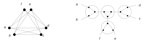
Figure 3. A graph of linear rank-width 2

3.3. Structure and obstructions

We will now discuss about some consequences of Theorem 1, particularly the structure of graphs of linear rank-width $1$.

Let $G$ be a graph and let $xy$ be an edge of $G$. The pivoting of $G$ on $xy$ is the graph $G*x*y*x=G*y*x*y$ [5, 18]. A graph $H$ is a pivot-minor of a graph $G$ if $H$ can be obtained from $G$ by a sequence of pivotings and deletions of vertices. It is clear that a pivot-minor is also a vertex-minor. A graph $H$ is a vertex-minor (or pivot-minor or induced subgraph) obstruction for linear rank-width $1$ if $H$ has linear rank-width $2$ and every proper vertex-minor (or pivot-minor or induced subgraph) of $H$ has linear rank-width $1$. In [1] the authors gave the induced subgraph (or vertex-minor or pivot-minor) obstructions for linear rank-width $1$. We will explain how to obtain all these obstructions in a more direct way from Theorem 1. The proof of the following is straightforward from Theorem 1.

Proposition 4.

A graph $G$ is a distance hereditary graph obstruction for linear rank-width $1$ if and only if its split decomposition tree is a star with three leaves and every connected component of every proper induced subgraph of $G$ has a path as split decomposition tree.

From Theorem 1, we can also deduce that if a connected graph has linear rank-width $1$, then for each internal node $u$ of $T_{G}$, $V(u)\neq\emptyset$ (recall that $V(u)$ is the set of vertices of $G$ in the block $b_{G}(u)$). Bouchet [5] characterises exactly distance hereditary graphs such that each internal node of the split decomposition tree contains at least one vertex.

Theorem 4 ([5]).

A distance hereditary graph $G$ is locally equivalent to a tree if and only if, for every internal node $u$ of $T_{G}$, $V(u)\neq\emptyset$. This tree is moreover unique.

In the following we deduce some interesting characterisations of graphs of linear rank-width $1$ we can deduce from Theorem 1 and some results in the literature.

Corollary 1.

Let $G$ be a connected graph. The following statements are equivalent.

1. $G$ is distance hereditary and $T_{G}$ is a path.

2. $G$ has linear rank-width $1$.

3. $G$ is locally equivalent to a caterpillar.

4. $G$ is a vertex-minor of a path.

5. $G$ does not contain neither the co-$(3K_{2})$ graph nor the Net graph nor the $5$-cycle as a vertex-minor.

Proof.

The equivalence between (1) and (2) is from Theorem 1. The equivalence between (2) and (4) is proved in [16], but can be easily proved from the equivalence between (2) and (3). Indeed, connected vertex-minors of paths have linear rank-width $1$ and since every caterpillar is a vertex-minor of a path, we are done.

The equivalence between (2) and (5) is proved in [1]. Let us explain how to prove it in a more direct way from Proposition 4. It is sufficient to construct the set of induced subgraph obstructions since the set of vertex-minor and pivot-minor obstructions can be derived from that set. The set of induced subgraph obstructions to being a distance hereditary graph is known for a while [3] and constitutes a subset of the induced subgraph obstruction for linear rank-width $1$. We now explain how to construct the set of distance hereditary induced subgraph obstructions for linear rank-width $1$. Let $H$ be a distance hereditary obstruction for linear rank-width $1$. From Proposition 4 its split decomposition tree $T_{H}$ is a star with three leaves, say centred at $v$ with $v_{1},v_{2}$ and $v_{3}$ as leaves. The following three cases describe exactly the canonical split decomposition of $H$.

Case 1: $b_{H}(v)$ is a clique. Then $b_{H}(v)$ has exactly three vertices and none of the $b_{H}(v_{i})$s is a clique. Moreover, for each $1\leq i\leq 3$ the graph $b_{H}(v_{i})$ has three vertices and is a star.

Case 2: $b_{H}(v)$ is a star centred at a marker vertex. Then $b_{H}(v)$ has three vertices. Let us assume without loss of generality that the centre of $v$ is the neighbour marker of the marker vertex in $v_{1}$. Then $b_{H}(v_{1})$ is either a clique or a star centred at a marker vertex, and for each $2\leq i\leq 3$ the graph $b_{H}(v_{i})$ has three vertices and is either a clique or a star centred at a vertex of $H$.

Case 3: $b_{H}(v)$ is a star centred at a vertex of $H$. Then $b_{H}(v)$ has four vertices and its centre is a vertex of $H$. Moreover, for each $1\leq i\leq 3$ the graph $b_{H}(v_{i})$ has three vertices and is either a clique or a star centred at a vertex of $H$.

From the description of the split decomposition of an induced subgraph obstruction for linear rank-width $1$, one can clearly construct all the induced subgraph obstructions for linear rank-width $1$. In Figure 4 we have recalled the vertex-minor obstructions for linear rank-width $1$. See [1] for the complete list of pivot-minor and induced subgraph obstructions for linear rank-width $1$.

It remains now to prove the equivalence between (2) and (3). Caterpillars have clearly linear rank-width $1$ and are the only trees with paths as split decomposition trees. Now if a graph $G$ has linear rank-width $1$, then from Theorem 1 it is a distance hereditary graph and its split decomposition tree $T_{G}$ is a path and each node $u$ is such that $V(u)\neq\emptyset$. By Theorem 4 it is then locally equivalent to a tree, say $T$. By [5, Theorem 4.4] $T_{G}$ is also the split decomposition tree of $T$, which concludes the proof. ∎

Figure 4. Forbidden vertex-minors for linear rank-width $1$ graphs. a) co-($3K_{2}$) b) Net and c) $C_{5}$.

3.4. Recognition algorithm

Thanks to the previous characterisations, graphs of linear rank-width $1$ can be recognised in time $O(n+m)$.

Theorem 5.

One can decide in time $O(n+m)$ if a connected graph $G$ with $n$ vertices and $m$ edges have linear rank-width $1$, and if not construct an obstruction. A linear ordering of cutrank $1$ can be constructed also in time $O(n+m)$ if it exists.

Proof.

Let $G$ be a graph with $n$ vertices and $m$ edges. Thanks to [12] one can check in time $O(n+m)$ if $G$ is a distance hereditary graph and if not exhibit an induced subgraph obstruction. From the induced subgraph obstruction one can exhibit, if he prefers, vertex-minor or pivot-minor obstructions.

We will now assume that $G$ is distance hereditary. We first construct a split decomposition tree $T_{G}$ of $G$ which can be done in time $O(n+m)$ [11]. By Theorem 1 $G$ has linear rank-width $1$ if and only if $T_{G}$ is a path. Since testing whether $T_{G}$ is a path can be done in time $O(|V(T_{G})|)=O(n)$, we can test in time $O(n+m)$ if $G$ has linear rank-width at most $1$. Knowing that $T_{G}$ is a path, one can construct a linear ordering of $V(G)$ of cutrank $1$ in time $O(n)$ by Proposition 2.

We now explain how to exhibit an induced subgraph obstruction if $T_{G}$ is not a path since from an induced subgraph obstruction one can exhibit a vertex-minor or a pivot-minor obstruction. If $T_{G}$ is not a path, then there exists an internal node $v$ of degree at least three, that can be found in time $O(n)$, and let us choose three of its neighbour nodes say $v_{1},v_{2},v_{3}$. We need to look at the type of the node $v$.

Case 1: $b_{G}(v)$ is a clique. Then none of the $v_{i}$s is a clique. In each of the graphs $G^{v_{i}v}$ take either two non adjacent vertices that are adjacent to vertices in $V(G)\setminus V(G^{v_{i}v})$ or two adjacent vertices such that exactly one is adjacent to vertices in $V(G)\setminus V(G^{v_{i}v})$.

Case 2: $b_{G}(v)$ is a star centred at a marker vertex. We may assume without loss of generality in this case that there exists a marker vertex in $v_{1}$ which is a neighbour marker of the centre of $b_{G}(v)$. Choose in $V(G)\setminus V(G^{v_{1}v})$ either two adjacent vertices or two non adjacent vertices, and in each of the graphs $G^{v_{i}v}$, for $2\leq i\leq 3$ choose two adjacent vertices such that at least one is adjacent to a vertex in $V(G)\setminus V(G^{v_{i}v})$.

Case 3: $b_{G}(v)$ is a star centred at a vertex of $G$. Take the centre of $b_{G}(v)$, and choose in each of the graphs $G^{v_{i}v}$ two adjacent vertices such that at least one is adjacent to a vertex in $V(G)\setminus V(G^{v_{i}v})$.

One checks easily that in each of the cases above the split decomposition tree of the chosen induced subgraph is a star with three leaves and is minimal with respect to that property, hence is an induced subgraph obstruction. ∎

March 17, 2024

References

- [1] Isolde Adler, Arthur M. Farley, and Andrzej Proskurowski, Obstructions for linear rank-width at most , To appear in Discrete Applied Mathematics (2013).
- [2] Isolde Adler and Mamadou Moustapha Kanté, Linear rank-width and linear clique-width of trees, WG, 2013.
- [3] Hans-Jürgen Bandelt and Henry Martyn Mulder, Distance-hereditary graphs, Journal of Combinatorial Theory, Series B 41 (1986), no. 2, 182–208.
- [4] André Bouchet, Digraph decompositions and eulerian systems, SIAM Journal on Algebraic and Discrete Methods 8 (1987), no. 3, 323–337.
- [5] by same author, Transforming trees by successive local complementations, Journal of Graph Theory 12 (1988), no. 2, 195–207.
- [6] by same author, Circle graph obstructions, Journal of Combinatorial Theory, Series B 60 (1994), no. 1, 107–144.
- [7] Bruno Courcelle, The monadic second-order logic of graphs XVI : Canonical graph decompositions, Logical Methods in Computer Science 2 (2006), no. 2.
- [8] Bruno Courcelle and Stephan Olariu, Upper bounds to the clique width of graphs, Discrete Applied Mathematics 101 (2000), no. 1-3, 77–114.
- [9] Bruno Courcelle and Sang-il Oum, Vertex-minors, monadic second-order logic, and a conjecture by seese, Journal of Combinatorial Theory, Series B 97 (2007), no. 1, 91–126.
- [10] William H. Cunnigham and Jack Edmonds, A combinatorial decomposition theory, Canadian Journal of Mathematics 32 (1980), 734–765.
- [11] Elias Dahlhaus, Parallel algorithms for hierarchical clustering, and applications to split decomposition and parity graph recognition, Journal of Algorithms 36 (2000), no. 2, 205–240.
- [12] Guillaume Damiand, Michel Habib, and Christophe Paul, A simple paradigm for graph recognition: application to cographs and distance hereditary graphs., Theoretical Computer Science 263 (2001), no. 1-2, 99–111.
- [13] Reinhard Diestel, Graph Theory (Graduate Texts in Mathematics), Springer, 2005.
- [14] Robert Ganian, Thread graphs, linear rank-width and their algorithmic applications, IWOCA (Costas S. Iliopoulos and William F. Smyth, eds.), Lecture Notes in Computer Science, vol. 6460, Springer, 2010, pp. 38–42.
- [15] Petr Hlinený and Sang il Oum, Finding branch-decompositions and rank-decompositions, SIAM J. Comput. 38 (2008), no. 3, 1012–1032.
- [16] O joung Kwon and Sang il Oum, Graphs of small rank-width are pivot-minors of graphs of small tree-width, To appear in Discrete Applied Mathematics (2013).
- [17] Mamadou Moustapha Kanté and Michaël Rao, Directed rank-width and displit decomposition, WG (Christophe Paul and Michel Habib, eds.), Lecture Notes in Computer Science, vol. 5911, 2009, pp. 214–225.
- [18] Sang-Il Oum, Graphs of bounded rank width, Ph.D. thesis, Princeton University, 2005.
- [19] by same author, Rank-width and vertex-minors., Journal of Combinatorial Theory, Series B 95 (2005), no. 1, 79–100.
- [20] Sang-Il Oum and Paul D. Seymour, Approximating clique-width and branch-width., Journal of Combinatorial Theory, Series B 96 (2006), no. 4, 514–528.
- [21] Michaël Rao, Solving some np-complete problems using split decomposition, Discrete Applied Mathematics 156 (2008), no. 14, 2768–2780.
- [22] Neil Robertson and Paul D. Seymour, Graph minors. I. excluding a forest, Journal of Combinatorial Theory, Series B 35 (1983), no. 1, 39–61.
- [23] by same author, Graph minors. II. algorithmic aspects of tree-width, Journal of Algorithms 7 (1986), no. 3, 309–322.