Remarks on the statistical aspects of the safety analysis

Abstract.

We investigate the statistical methods applied throughout safety analysis of complex systems. The tolerance interval method implemented in the widely utilized 0.95—0.95 methodology is analyzed. We point out a remarkable weakness of the tolerance interval method concerning the principle of repeatability. It is proved that repeating twice the procedure, the probability that the second maximum will be larger/smaller than the first one is 50%. This statement is not surprising, it holds for any random variable with continuous distribution function. In order to demonstrate the undesirable consequences of the tolerance interval method in the decision making, the results of the analysis of an elementary example are discussed. Instead of the tolerance interval method, we suggest another method based on the sign test which has more encouraging features, especially in the case of several output variables. The problematic aspects of the method are also discussed. Finally, we suggest a simple test case which is able to reveal if the tolerance interval method would not be capable of determining the risky states of the system, when there are only a few of them. If there are many, then the method may not explore each one in the analysis.

1. Introduction

Regulation of industrial devices prescribes an analysis of the risk associated with the operation of the device. The US regulation (10CFR 50.46), which is considered as standard world wide, fixes the requirement that the analyst should conclude ”with high probability” that the device is safe. At the same time, one can add further self-explaining requirements, like

• Repeatability: when the analysis is repeated one should get more or less the same safety limits or other relevant safety features;

• Objectivity: the analysis should be based on scientific considerations, not on individual considerations. This assumes that principles of safety analysis are widely discussed and approved by experts.

• Transparency of the procedure: The safety analysis is prepared by a group of experts, and is discussed by experts of several professions. It should be assured that there are participants in the discussion who are capable of providing pieces of information on every relevant and major areas of the safety analysis (plant data, design principles, and methodology of the analysis).

The first two items touch the safety analysis itself, whereas the third one touches rather organizational problems. The present work deals with the first two items. The analyst [1] may utilize the best estimate method with uncertainty analysis. Here a possible approach is to select a device (e.g. a nuclear reactor, chemical reactor) with nominal parameters and to specify those parameters which are involved in the uncertainty analysis. In the course of the analysis, the analyst selects a possible realization of the device by replacing the nominal parameters by actual parameters and calculates the parameters to be subjected to limitations. We call this procedure a run. The actual parameters are drawn from a probability distribution determined by engineering judgement.

We are going to point out that the traditional $0.95|0.95$ tolerance interval method fails to be repeatable and objective because the repeated code runs may lead to considerable differences in the obtained maxima. In a considerable portion of the cases repeating for instance twice the run, the probability that the maximum obtained in the second run will be larger/smaller than in the first run is $1/2$. This statement is not at all surprising, since it holds for any random variable with continuous distribution function. The problem is that the random nature of the maximal value is often disregarded in practice.

We point out the weakness of the $0.95|0.95$ methodology by presenting a simple example in which the ”code for simulation” is replaced by random outputs obeying lognormal distribution, and analyze the properties of samples taken from these outputs.

Instead of the $0.95|0.95$ methodology we propose another statistical method, called sign test, which is a variant of the good old Clopper-Pearson [2] method. We claim that the method proposed by us has some advantages in comparison with the tolerance interval method, furthermore the erratic behavior of the coverage probability of the confidence interval [3] renders the method conservatism and puts the analyst on the safe side. The main advantage of the sign test method is nothing else than it is directly applicable in the case of several output variables.

Finally, we analyze a trivial test problem in the usual safety analysis frame: a series of calculations are performed by a numerical model of the device. The analysis ought to verify that no limit violation occurs in any realistic device state. In the suggested test, limit violation occurs only in 1% of the possible states. The challenge is to pinpoint the risky states.

The structure of the present work is as follows. In Section 2, we analyze the random nature of the maximal values of the sample set produced by runs of a code as it is usually done with any best estimate method. In Section 3, we present an elementary example to point out the drawbacks of this method. The sign test is discussed in Section 4, and in Section 5, we recommend a simple test to verify the statistical methods to be applied in statistical inference used in safety analysis. Conclusions are given in Section 6.

2. Features of the tolerance interval method

We are going to analyze the safety of a device. It is assumed that there is a computer model associated with the device. The computer model is assumed to be a best estimate model. In the first step the major uncertain input parameters should be identified, their probability density functions have to be determined, usually by engineering judgement. The model provides us with output variables which are random variables because of the random input these are subject to limitations. The joint probability distribution function of the output is unknown. By repeatedly running the code, the analyst obtains a data set representing the operation of the device which is regarded now a ”black box” device. By exploiting the information in the data set, the analyst tries to make a decision whether the device is safe or not. Generally accepted, that the tolerance interval method, known simply under the name $0.95|0.95$ methodology, can be used for this purposes. In former papers [4], [5] we discussed the tolerance interval method in detail. In the present article, we will use only a simple version of the mentioned method to demonstrate its weakness arising because of a random parameter involved in the safety criteria. Unfortunately most analysts neglect aftermath of that fact.

Before discussing the statistical aspects of the problem, we sum up the analyst’s riddle. With the code at his disposal, the analyst determines the parameters under limitation. The key question is: whether the calculated parameters exceed the limits or not. In the analysis a major problem is that the device is not exactly determined, the device parameters lie in an interval. This is taken into account by selecting randomly the actual state of the device. The question is: had we repeat the calculations with different parameters, would we have get a more risky state or not? The resolution of the analyst problem is based on statistical considerations and is given below.

Let $y$ be a single random output, which is subject to limitation. Let the acceptance range be given as $(-\infty,U_{T}]$, where $U_{T}$ is the technological limit for $y$. We assume that the distribution of $y$ is unknown, and are looking for a quantile $Q_{\gamma}$ such that

(2.1) $$\int_{-\infty}^{Q_{\gamma}}dG(y)=\gamma,$$

where $G(y)$ is the cumulative distribution function of the output variable $y$. Quantile $Q_{\gamma}$ is to be estimated from calculations, thus, itself is a random variable. Let us consider the results of $N$ runs of a code modeling the output variable $y$. The $N$ values obtained in $N$ runs form a sample, and let us produce $n+1$ samples. The first sample $y_{01},y_{02},\cdots,y_{0N}$ will be called basic sample. Introducing the ordered samples

$$y_{k}(1)<y_{k}(2)<\cdots<y_{k}(N),\;\;\;\;\;\;\mbox{where}\;\;\;\;\;\;k=0,1,\ldots,n,$$

we can write the sample elements into the following $(n+1)\times N$ matrix:

(2.2) $$\begin{array}[]{cccc}y_{0}(1)&y_{0}(2)&\cdots&y_{0}(N)\\ y_{1}(1)&y_{1}(2)&\cdots&y_{1}(N)\\ \cdots&\cdots&\cdots&\cdots\\ y_{n}(1)&y_{n}(2)&\cdots&y_{n}(N),\end{array}$$

in which we call the first row the ordered basic sample. Assuming that the unknown cumulative distribution function $G(y)$ is monotonously increasing and continuous, it can be immediately proved the well known statement that

(2.3) $$\mathcal{P}\left\{y_{k}(N)>G^{-1}(\gamma)\right\}=\mathcal{P}\left\{\int_{-\infty}^{y_{k}(N)}dG(y)>\gamma\right\}=1-\gamma^{N}=\beta,$$

where $G^{-1}(\gamma)=Q_{\gamma}$ is the $\gamma$-quantile of the probability distribution function $G(y)$. In other words, any upper sided interval $[-\infty,y_{k}(N)]$ covers more than the $\gamma$-quantile $Q_{\gamma}$ of the output variable $y$ with probability $\beta$. 

Since one finds misinterpretations in the engineering practice it is not superfluous to underline once again the proven notion of formula (2.3). $\beta$ is the probability that the largest value $y_{k}(N)$ of the $k$th sample comprising $N$ output values is greater then the $\gamma$ quantile of the unknown distribution $G(y)$ of the output variable $y$. Another formulation asserts that $\beta$ is the probability that the interval $[-\infty,y_{k}(N)]$ covers a larger than $\gamma$ portion of the unknown probability distribution function. The $\gamma$ is often called as probability content and $\beta$ as confidence level.

The maximal values $y_{0}(N),y_{1}(N),\ldots,y_{n}(N)$ are independent and identically distributed nonnegative continuous random variables. Hence, if $k\not=\ell$, where $k\leq n$ and $\ell\leq n$ are nonnegative integers, then the probability of the event $\left\{y_{k}(N)<y_{\ell}(N)\right\}$ is equal to that of the event $\left\{y_{k}(N)>y_{\ell}(N)\right\}$, and one obtains immediately that

(2.4) $${\mathcal{P}}\left\{y_{k}(N)<y_{\ell}(N)\right\}={\mathcal{P}}\left\{y_{k}(N)>y_{\ell}(N)\right\}=\frac{1}{2}.$$

Introduce the notation

(2.5) $${\mathcal{P}}\left\{y_{k}(N)<y\right\}={\mathcal{P}}\left\{\max_{1\leq j\leq N}y_{kj}\leq y\right\}=\prod_{j=1}^{N}{\mathcal{P}}\left\{y_{kj}\leq y\right\}=\left[G(y)\right]^{N}=H(y),$$

$$k=0,1,\ldots,n,$$

one can write that

$${\mathcal{P}}\left\{y_{k}(N)<y_{\ell}(N)\right\}=\int_{-\infty}^{+\infty}\left[1-H(y)\right]\;dH(y)=\frac{1}{2}$$

and similarly

$${\mathcal{P}}\left\{y_{k}(N)>y_{\ell}(N)\right\}=\int_{-\infty}^{+\infty}H(y)\;dH(y)=\frac{1}{2}.$$

From the equation (2.4), the trivial statement follows that the probability of finding the maximal value in a sample larger/smaller than in the previous one, is $1/2$.

Let $0\leq\nu_{n}(y)\leq n$ denote the number of those random variables from among

$$y_{1}(N),\ldots,y_{n}(N)$$

which are greater than $y$. Obviously,

(2.6) $$\mathcal{P}\left\{\nu_{n}(y)=\ell\right\}=J_{\ell}^{(n)}(y)=\binom{n}{\ell}\;\left[1-H(y)\right]^{\ell}\left[H(y)\right]^{(n-\ell)}.$$

Let $p_{\ell}^{(n)}$ stand for the probability that from among the random variables $y_{1}(N),\ldots,y_{n}(N)$ exactly $\ell\leq n$ is greater than $y_{0}(N)$, which may be any real number. We obtain from (2.6) that

(2.7) $$p_{\ell}^{(n)}=\int_{-\infty}^{+\infty}J_{\ell}^{(n)}(y\;dH(y)=\binom{n}{\ell}\;\int_{0}^{1}(1-u)^{\ell}\,u^{n-\ell}\;du=\frac{1}{n+1}.$$

Note, that the probability $p_{\ell}^{(n)}$ is independent of $\ell$.  The probability $P_{k}^{(n)}$, that at least $k\leq n$ out of maximal values $y_{1}(N),y_{2}(N),\ldots,y_{n}(N)$ will exceed the basic maximal value $y_{0}(N)$, can be calculated by using the formula (2.7). We have that

(2.8) $$P_{k}^{(n)}=\sum_{\ell=k}^{n}p_{\ell}^{(n)}=\frac{n+1-k}{n+1}=1-\frac{k}{n+1},$$

which is independent of $\gamma$ and $\beta$. In the sequel the larger/smaller statements will be used only in their ”larger” interpretation.

Let $\lambda$ be the number of those $y_{1}(N),y_{2}(N),\ldots,y_{n}(N)$ variables which are larger than the basic $y_{0}(N)$. Clearly, $\lambda$ is a random variable, its expectation value is

(2.9) $$\mathbf{E}\{\lambda\}=\sum_{\ell=1}^{n}\ell\;p_{\ell}^{(n)}=\frac{n}{2},$$

and its variance is

$$\mathbf{D}^{2}\{\lambda\}=\sum_{\ell=1}^{n}\left(\ell-n/2\right)^{2}\;p_{\ell}=\frac{1}{6}\,\left(1+\frac{n}{2}\right).$$

As a consequence, we see that the expectation of the number of maximal values out of $n$ samples, that will exceed the basic maximal value $y_{0}(N)$, is 50% of $n$, i.e. repeating the run many times we may expect maximal values higher than the basic maximal value in every second case.

In the light of this statement one asks: is this the intended outcome of the $0.95|0.95$ methodology? A further serious objection to the $0.95|0.95$ methodology is the absence of the uniqueness.

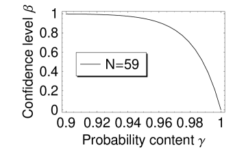
Figure 1. Dependence of the confidence level $\beta$ on the probability content $\gamma$ for sample size $N=59$.

In Fig. 1 on can see the dependence of the confidence level $\beta$ on the probability content $\gamma$ for sample size $N=59$. The statement that the maximal element in a sample obtained by $N=59$ runs is higher than the unknown quantile $Q_{0.95}$ with probability $0.95$ is equivalent, for instance, to the statement that the maximal element is higher than the unknown quantile $Q_{0.98}$ but with probability $0.7$. It is clear that there are infinite many $\beta|\gamma$ pairs corresponding to the same $N$ value. In the safety analysis the $0.95|0.95$ pair is accepted but not mentioned that other pairs are also allowed.

3. A witness of the weakness

In order to demonstrate the weakness of the tolerance interval method , we consider a rather simple example. Take a single output variable $y$ of lognormal distribution  with parameters $m$ and $d$. This plays the role of our ”unknown” $G(y)$ distribution. The density function is

(3.1) $$g(y)=\frac{1}{yd\sqrt{2\pi}}\exp\left[-\frac{1}{2}\left(\frac{\log y-m}{d}\right)^{2}\right],$$

where $y\geq 0$.

We carried out the following numerical experiment. By means of Monte Carlo simulation we generated samples of size $N=59$. In the simulation we have taken $m=2.5$ and $d=0.5$. As mentioned before, we call the first sample generated by $N=59$ runs the basic sample, the maximal element of which is denoted by $y_{0}(59)$. Then, we repeat the sample generation $n=1000$ times, and select the maximal value out of each sample. We obtained a series

$$y_{1}(59),\ldots,y_{1000}(59)$$

of the upper limits of the one-sided tolerance intervals which cover the $95$% of the distribution with probability $\beta=0.95$.

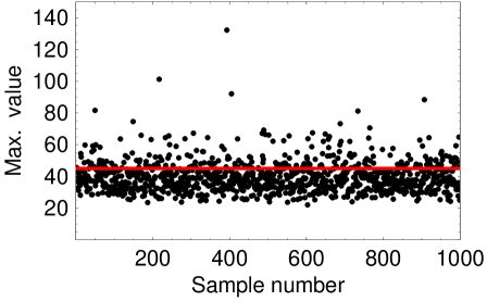
Figure 2. Maximal values of $1000$ samples of size $N=59$. The maximal value of the basic sample is $y_{0}(59)\approx 45$ and denoted by red line.

The maximal values of samples are shown in Fig. 2. The maximum in the basic sample is $y_{0}(59)\approx 45$. The lowest of the maximal values in the experiment is $22.04$, while the largest is $132.27$. One can observe that in $234$ cases (more than $23$% of the one thousand samples) the maximum exceeds $y_{0}(59)\approx 45$.

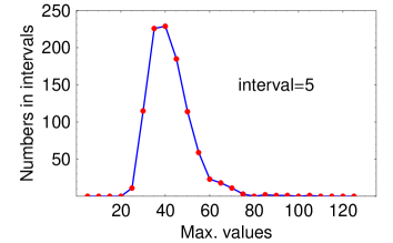
Figure 3. Distribution of the maximal values of $1000$ samples of size $N=59$ in intervals of length $5$.

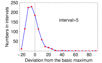
Figure 4. Distribution of the deviations of the maximal values from the basic maximum $45$ in intervals of length $2.5$.

In order to visualize better the random behavior of the maxima, we condensed the maxima, and counted the frequency of maxima falling into $[(i-1)*5,i*5],i=1,\dots 200$. That empirical distribution is shown in Fig. 3. Fig. 4 shows the difference $y_{k}(59)-y_{0}(59)$.

Let us check now if these properties are comply with the statistics. The probability that the largest element in a given sample is greater than $Q_{\gamma}$ is $1-\gamma^{N}$. Let $\xi_{n}(Q_{\gamma})$ stand for the random variable giving the number of maximum elements exceeding $Q_{\gamma}$. The probability distribution of the newly introduced random variable is

(3.2) $${\mathcal{P}}\{\xi_{n}(Q_{\gamma})=k\}=\binom{n}{k}\;(1-\gamma^{N})^{k}\;\gamma^{N(n-k)}.$$

From this expression we obtain the expectation value and the variance as

(3.3) $${\mathbf{E}}\{\xi_{n}(Q_{\gamma})\}=n(1-\gamma^{N}),$$

(3.4) $${\mathbf{D}}^{2}\{\xi_{n}(Q_{\gamma})\}=n\;\gamma^{N}\;(1-\gamma^{N}).$$

When $n$ and $k$ are sufficiently large, the distribution of the random variable

(3.5) $$\chi_{n}(Q_{\gamma})=\frac{\xi_{n}(Q_{\gamma})-{\bf E}\{\xi_{n}(Q_{\gamma})\}}{{\bf D}\{\xi_{n}(Q_{\gamma})\}}$$

is approximately standard normal, hence,

(3.6) $${\mathbf{E}}\{\xi_{n}(Q_{\gamma})\}-\kappa\;{\mathbf{D}}\{\xi_{n}(Q_{\gamma})\}\leq\xi_{n}(Q_{\gamma})\leq{\mathbf{E}}\{\xi_{n}(Q_{\gamma})\}+\kappa\;{\mathbf{D}}\{\xi_{n}(Q_{\gamma})\}$$

is valid with probability $w$, and $\kappa$ is the root of the equation

(3.7) $$\frac{1}{\sqrt{2\pi}}\;\int_{-\infty}^{\kappa}e^{-u^{2}/2}\;du=\frac{1+w}{2}.$$

Substituting here $n=1000$, $N=59$, $\gamma=0.95$ and $w=0.95$, we get $\mathbf{E}\{\xi_{n}(Q_{\gamma})\}\approx 952,\;\mathbf{D}\{\xi_{n}(Q_{\gamma})\}\approx 6.79$, and $\kappa\approx 1.96$. The inequality (3.6) is given by

$$938<\xi_{1000}(Q_{0.95})<964,$$

where $\xi_{1000}(Q_{0.95})\approx 940$. This relationship is witnessing the correctness of the statistics. In spite of the nice agreement we wish to underline that the $0.95|0.95$ methodology does not exclude rare events such as limit violation when some of the calculated values are over the technological limit $U_{T}$.

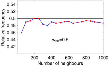
Figure 5. Relative frequency of the event $y_{\ell-1}(59)<y_{\ell}(59)$ in $50,100,\ldots,1000$ neighbors.

To illustrate that the probability of finding a larger maximal value in a sample than in the previous one, is $w_{nb}=0.5$, we have used the maximums in $1000$ samples of size $59$ and have calculated the relative frequencies of the event $y_{\ell-1}(59)<y_{\ell}(59)$ in $50(50)1000$ neighbors. The results of calculations are seen in Fig. 5.

One should emphasize that this behavior of the upper limit of the tolerance interval is not surprising, this is a well established consequence of the random nature of the maximal values selected from the samples. It seems to be justified the need that the tolerance interval method has to be replaced by a more reliable method, if it is possible at all.

4. Method based on sign test

The concluding remarks at the end of the previous section are not optimistic. The question whether one can find a suitable check, which is based on a computer model, on the safety of a large device cannot be answered satisfactorily. Below we propose a method, borrowed from Kendall’s book [6], called ”sign test” which may be more adequate than the 0.95/0.95 method.

4.1. Single output variable

Again, we assume the cumulative distribution function $G(y)$ of the output variable to be continuous but unknown. Let $S_{N}=\{y_{1},\ldots,y_{N}\}$ be a sample of $N$ observations (runs of a computer model). Define the function

(4.1) $$\Delta(x)=\left\{\begin{array}[]{ll}1,&\mbox{if $x>0$,}\\ \mbox{}&\mbox{}\\ 0,&\mbox{if $x<0$,}\end{array}\right.$$

and introduce the statistical function

(4.2) $$z_{N}=\sum_{k=1}^{N}\Delta(U_{T}-y_{k})$$

which gives the number of sample elements smaller than the safety level $U_{T}$ by declaring that any state of the device with output smaller than $U_{T}$ is safe. Criteria based on statistical function (4.2) are called sign criterion since $z_{N}$ counts only the positive $U_{T}-y_{k}$ differences. When $G(y)$ is continuous, the probability of $U_{T}-y=0$ is surly zero.

Obviously, distribution of $z_{N}$ is binomial, using the notation

(4.3) $${\mathcal{P}}\{\Delta(U_{T}-y)=1\}={\mathcal{P}}\{y\leq U_{T}\}=p,$$

we obtain

(4.4) $${\mathcal{P}}\{z_{N}=k\}=\binom{N}{k}\;p^{k}\;(1-p)^{N-k},\;\;\;\;\;\;k=0,1,\ldots,N.$$

The decisive parameter is the probability $p$ which can be called safety probability, and our task is to find a confidence interval $[\gamma_{L}(k),\;\gamma_{U}(k)]$ that covers the value $p$ with a prescribed probability $\beta$ provided we have a sample of size $N$ and in the sample $z_{N}=k\leq N$ elements smaller than the safety level $U_{T}$. The mathematics of the problem is well known, and one can find a large number of publications [7] - [11] in this field. However, there are several special aspects of the safety analysis, which need some further considerations.

Clearly, the formula (4.3) gives the probability that the output $y$ is not larger than the safety level $U_{T}$. When the lower limit $\gamma_{L}(k)$ of the confidence interval is close to unity, we can claim at least with probability $\beta$ that the chance of finding the output $y$ smaller than $U_{T}$ is also close to unity and the device under consideration, in its output $y$, can be regarded as safe at the level $[\beta|\gamma_{L}(k)]$.

If the sample size $N>50$, the random variable

(4.5) $$\frac{k-Np}{\sqrt{Np\;(1-p)}}=\zeta_{k}$$

has approximately normal distribution. Here $k$ is the number of sample elements not exceeding $U_{T}$. Let $\beta$ denote the confidence level, then

$${\mathcal{P}}\{|\zeta_{k}|\leq u_{\beta}\}=2\Phi(u_{\beta})-1=\beta,$$

where $\Phi(x)$ is the standard normal distribution function. This equation can be rewritten in the form

$${\mathcal{P}}\{|\zeta_{k}|\leq u_{\beta}\}={\mathcal{P}}\{(N+u_{\beta}^{2})(p-\gamma_{L})(p-\gamma_{U})\leq 0\}=\beta,$$

where

$$\gamma_{L}=\gamma_{L}(k,u_{\beta})=$$

(4.6) $$=\frac{1}{N+u_{\beta}^{2}}\;\left[k+\frac{1}{2}u_{\beta}^{2}-u_{\beta}\sqrt{k(1-k/N)+u_{\beta}^{2}/4}\right],$$

and

$$\gamma_{U}=\gamma_{U}(k,u_{\beta})=$$

(4.7) $$=\frac{1}{N+u_{\beta}^{2}}\;\left[k+\frac{1}{2}u_{\beta}^{2}+u_{\beta}\sqrt{k(1-k/N)+u_{\beta}^{2}/4}\right].$$

Here $u_{\beta}$ is the root of

$$\Phi(u_{\beta})=\frac{1}{2}(1+\beta).$$

In a number of cases it suffices to know the probability of the event $\{\gamma_{L}(k,v_{\beta})\leq p\}$, where $v_{\beta}=\Phi^{-1}(\beta)$. Since $\zeta_{k}$ with fixed $k$ is a decreasing function of $p$, the events $\{\zeta_{k}\leq v_{\beta}\}$ and $\{\gamma_{L}(k,v_{\beta})\leq p\}$ are equivalent, hence

$${\mathcal{P}}\{\zeta_{k}\leq v_{\beta}\}={\mathcal{P}}\{\gamma_{L}(k,v_{\beta})\leq p\}=\Phi(v_{\beta})=\beta.$$

Consequently, the operation of a device can be regarded safe if the parameter $p$ for all output variables is covered by $[\gamma_{L}(k,v_{\beta}),1]$ with a prescribed probability $\beta$, provided that $\gamma_{L}(k,v_{\beta})$ is close to unity.

Table 1. Number of successes $k$ in a sample of size $N$

$k$	99	108	118	128	137	147	157	166	176	185	195
$N$	100	110	120	130	140	150	160	170	180	190	200

Table 1 gives the number of successes $k$ in a sample of size $N$ needed for acceptance at the level $\beta=\gamma_{L}=0.95$. We utilized the approximate formula (4.6) with $u_{\beta}\rightarrow v_{0.95}\approx 1.64$ to derive the entries in Table 1.

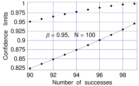
Figure 6. Dependence of $\gamma_{L}$ and $\gamma_{U}$ on the number of successes in a sample of N=100 elements.

When the sample size is less than $50$, we may not apply the asymptotically valid normal distribution. The below given derivation of the confidence limits is a modified version of the method proposed by Clopper and Pearson [2]. The probability of at least $k$ successes from $N$ observations is given by

$$S_{k}^{(N)}(p)=\sum_{j=0}^{k}\binom{N}{j}\;p^{j}\;(1-p)^{N-j},$$

where $p={\mathcal{P}}\{y\leq U_{T}\}$. This formula can be recast as

$$S_{k}^{(N)}(p)=\frac{N!}{k!\;(N-k-1)!}\;\int_{0}^{1-p}(1-v)^{k}\;v^{N-k-1}\;dv,$$

and it is clear from that expression that $S_{k}^{(N)}(p)$ is a monotonously decreasing function of $p$. Since

$$S_{k}^{(N)}(p)=\left\{\begin{array}[]{ll}1,&\mbox{if $p=0$,}\\ \mbox{}&\mbox{}\\ 0,&\mbox{if $p=1$,}\end{array}\right.$$

it assumes an arbitrary value only once in the interval [0,1]. Consequently, a $p=p_{\delta}$ value exists so that

$$S_{k}^{(N)}(p_{\delta})=\delta,\;\;\;\;\;\;\forall\;0<\delta<1.$$

Exploiting the monotony, we can construct a function such that

$$R_{k}^{(N)}(p)<R_{k}^{(N)}(p_{\delta})=\delta,$$

when $p>p_{\delta}$. Such a function is

$$R_{k}^{(N)}(p)=1-S_{k-1}^{(N)}(p)=\sum_{j=k}^{N}\binom{N}{j}\;p^{j}\;(1-p)^{N-j},$$

Finally, we establish the upper limit $\gamma_{U}$ from

(4.8) $$S_{k}^{(N)}(\gamma_{U})\leq\frac{1}{2}(1-\beta),$$

and the lower limit $\gamma_{L}$ from

(4.9) $$R_{k}^{(N)}(\gamma_{L})\leq\frac{1}{2}(1-\beta).$$

The interval $[\gamma_{L},\;\gamma_{U}]$ covers the unknown parameter $p$ with probability $\beta$. The dependence of $\gamma_{L}$ and $\gamma_{U}$ are shown in Fig. 6 for a sample of $N=100$ elements, $\beta$ stands for confidence level.

4.2. Several Output Variables

Now we assume the output to comprise $\ell$ variables. Let these variables be $y_{1},\ldots,y_{\ell}$. There are several fairly good test to prove if they are statistically independent or not. To each of the independent variables we can apply the considerations above but for dependent variables we need novel approach. Let

$$\mathbf{S}_{N}=\left(\begin{array}[]{cccc}y_{11}&y_{12}&\ldots&y_{1N}\\ y_{21}&y_{22}&\ldots&y_{2N}\\ \vdots&\vdots&\ddots&\vdots\\ y_{\ell 1}&y_{\ell 2}&\ldots&y_{\ell N}\end{array}\right)$$

denote the sample matrix obtained in $N>>\ell$ independent observations. With a computer model, an observation is a run. Introducing the column vector $\vec{y}_{k}$ of $\ell$ components, the sample matrix can be written as

$$\mathbf{S}_{N}=\left(\vec{y}_{1},\ldots,\vec{y}_{N}\right).$$

In accordance with our assumption, different vectors $\vec{y}_{k}$ are statistically independent but the components in a given vector may be dependent.

Below we expound the sign test only for two output variables $y_{1}$ and $y_{2}$ relying on the assumption that their joint distribution function $G(y_{1}$,$y_{2})$ is unknown but continuous in either variable. The goal of the foregoing analysis is to verify the safety conditions $y_{1}<U_{T}^{(1)}$ and $y_{2}<U_{T}^{(2)}$. When the conditions are accomplished with probability $p_{12}=G(U_{T}^{(1)},U_{T}^{(2)})\approx 1$ we say the device is safe for the outputs $y_{1}$ and $y_{2}$. Here, as before, the limits $U_{T}^{(1)}$, and $U_{T}^{(2)}$ are determined by technological requirements. Since $p_{12}$ is unknown, our job is to construct a confidence interval $[\gamma_{L}^{(1,2)},\;\gamma_{U}^{(1,2)}]$ so that it covers $p_{12}$ with probability $\beta_{12}$. In most cases it suffices to calculate solely the lower confidence limit $\gamma_{L}^{(1,2)}$, and to use the interval $[\gamma_{L}^{(1,2)},\;1]$ as confidence interval.

The event $\{y_{1k}<U_{T}^{(1)},\;y_{2k}<U_{T}^{(2)}\}$ will be called a success. Now, introduce the statistical function

$$z_{N}^{(1,2)}=\sum_{k=1}^{N}\Delta(U_{T}^{(1)}-y_{1k})\;\Delta(U_{T}^{(2)}-y_{2k})$$

which gives the number of successes in a sample of size $N$. Obviously, if $y_{1k}<U_{T}^{(1)}$ and $y_{2k}<U_{T}^{(2)}$, then

$$\Delta(U_{T}^{(1)}-y_{1k})\;\Delta(U_{T}^{(2)}-y_{2k})=1,$$

while $0$ otherwise. Since the newly introduced random variable $z_{N}^{(1,2)}$ is the sum of $N$ independent random variables, assuming values either 1 or 0, its distribution is binomial. Using the notation

$${\mathcal{P}}\{\Delta(U_{T}^{(1)}-y_{1})\;\Delta(U_{T}^{(2)}-y_{2})=1\}={\mathcal{P}}\{y_{1}<U_{T}^{(1)},\;y_{2}<U_{T}^{(2)}\}=p_{12},$$

we can write

$${\mathcal{P}}\{z_{N}^{(1,2)}=k\}=\binom{N}{k}\;p_{12}^{k}\;(1-p_{12})^{N-k},$$

for $k=0,1,\ldots,N$. Clearly, $p_{12}$ is the joint probability of safety for the output variables $y_{1}$ and $y_{2}$.

At this point we rejoin the thought of line of the previous subsection. Instead of repeating the already familiar argumentation, we amend two trivial although important remarks. Let us define the following two statistical functions:

$$z_{N}^{(1)}=\sum_{i=1}^{N}\Delta(U_{T}^{(1)}-y_{1i})\;\;\;\;\;\;\mbox{and}\;\;\;\;\;\;z_{N}^{(2)}=\sum_{j=1}^{N}\Delta(U_{T}^{(2)}-y_{2j}).$$

In general, these two functions are statistically not independent. Each of them is a sum of $N$ independent random variables with values 1 or 0, therefore, one can write

$${\mathcal{P}}\{z_{N}^{(1)}=i\}=\binom{N}{i}\;p_{1}^{i}(1-p_{1})^{N-i}$$

and

$${\mathcal{P}}\{z_{N}^{(2)}=j\}=\binom{N}{j}\;p_{2}^{j}(1-p_{2})^{N-j},$$

$$i,j=1,\ldots,N,$$

where

$$p_{\ell}={\mathcal{P}}\{y_{\ell}<U_{T}^{(\ell)}\}={\mathcal{P}}\{\Delta(U_{T}^{(\ell)}-y_{\ell})=1\},\;\;\;\;\;\;\ell=1,2,$$

are unknown probabilities of safety for output variables $p_{1}$ and $p_{2}$. Applying the method used previously, this time separately to the samples

$${\mathcal{S}}_{N}^{(1)}=\{y_{1i},\;\;i=1,\ldots,N\}\;\;\;\;\;\;\mbox{and}\;\;\;\;\;\;{\mathcal{S}}_{N}^{(2)}=\{y_{2j},\;\;j=1,\ldots,N\},$$

we construct two random intervals $[\gamma_{L}^{(1)},\;1]$ and $[\gamma_{L}^{(2)},\;1]$ covering $p_{1}$ and $p_{2}$ with probabilities $\beta_{1}$ and $\beta_{2}$, respectively. Evidently, it could occur that the levels $(\beta_{1}|\gamma_{L}^{(1)})$ and $(\beta_{2}|\gamma_{L}^{(2)})$ corroborate the claim that samples ${\mathcal{S}}_{N}^{(1)}$ and ${\mathcal{S}}_{N}^{(2)}$ separately comply with safety requirements. However, this does not mean that we would arrive at the same conclusion from analyzing the two samples jointly. The reason is that $y_{1}$ and $y_{2}$, the two output random variables are statistically in general not independent. Hence, we should ascertain weather the interval $[\gamma_{L}^{(1,2)},\;1]$ covers the probability $p_{12}$ with the pre-assigned probability $\beta_{12}$.

Decision on the safety, when two output variables are subjected to limitations should go as follows. Firstly, we test the hypothesis concerning dependence of the output variables $y_{1}$ and $y_{2}$. If they are dependent, we should estimate the random interval $[\gamma_{L}^{(1,2)},\,1]$ which covers $p_{12}$ with probability $\beta_{12}$. Solely if they are statistically independent should we estimate the random intervals $[\gamma_{L}^{(1)},\,1]$ and $[\gamma_{L}^{(2)},\,1]$ covering $p_{1}$ and $p_{2}$ with probabilities $\beta_{1}$ and $\beta_{2}$, respectively.

For the sake of demonstration, an example is given below. First, the lower confidence limits are calculated for the parameter $p$ as a function of the success number $k$, in the case of sample size $N=100$, at the confidence levels $\beta=0.9,0.95$ and $0.99$.

Table 2. Lower confidence limits in a sample of $N=100$ as a function of the success number $k$ at three confidence levels $\beta$

$k$ $\backslash$ $\beta$	0.90	0.95	0.99
90	0.8501	0.8362	0.8086
91	0.8616	0.8482	0.8212
92	0.8733	0.8602	0.8340
93	0.8850	0.8725	0.8471
94	0.8970	0.8850	0.8604
95	0.9092	0.8977	0.8741
96	0.9216	0.9108	0.8882
97	0.9344	0.9242	0.9030
98	0.9476	0.9383	0.9185
99	0.9616	0.9534	0.9354
100	0.9772	0.9704	0.9549

Then, by using Monte Carlo simulation, we have generated two samples a) and b) either sample contains $N=100$ observations (runs) of two output variables. The samples have been generated from a bivariate normal distribution with parameters $m_{1}=m_{2}=0$ and $\sigma_{1}=\sigma_{2}=1$ but the correlation coefficient is $C=0.1$ in the sample a) while that is $C=0.7$ in the sample b). The acceptance range is $[-2,2]$ for both output variables. In sample a) and b) $4$ and $2$ samples lie respectively outside the acceptance range.

Figure 7. Sample a)

Figure 8. Sample b)

First let us consider the sample a). It can be seen that the number of successes among $100$ events is $96$, i.e. the number of safety violation is $4$. From Table 2 one can read in this case that the interval [0.9108,1] covers the parameter $p_{12}$ with probability $\beta_{12}=0.95$. This coverage is rather small to state the device is safe. When we assess the output variables one by one, we see that the associated parameters $p_{1}$ and $p_{2}$ are covered by the interval $[0.9383,1]$ with probability $\beta=0.95$ in either sample. However tempting is to accept $0.9383$ as lower bound for the probability to be used in safety analysis, that number has nothing to do with $p_{12}$ and should not be used in safety analysis.

Now let us pass on to sample b) where we see a strong correlation between $y_{1}$ and $y_{2}$. The number of safety violations is $2$ and from Table 2 one can read that the confidence interval $[0.9383,1]$ covers the parameter $p_{12}$ with probability $\beta_{12}=0.95$. In other words, we conclude that the probability of the event $\{y_{1}<U_{T}^{(1)},\;y_{2}<U_{T}^{(2)}\}$ is at least $0.9383$. Since there is only $1$ violation for both output variables $y_{1}$ and $y_{2}$, according to Table 2 the parameters $p_{1}$ and $p_{2}$ are covered by the same interval $[0.9534,1]$ on the level $\beta_{1}=\beta_{2}=0.95$. Again, however favorable these numbers are, they should not be used in assessing safety. The above discussed simple numerical example clearly indicated the danger awaiting the analyst when his/her judgment is based on tests performed separately on correlated output variables.

Finally, we mention that the generalization of the sign test to $\ell>2$ output variables is straightforward, we have to use the statistical function

(4.10) $$z_{N}^{(1,\ldots,\ell)}=\sum_{k=1}^{N}\;\prod_{j=1}^{\ell}\Delta(U_{T}^{(j)}-y_{jk})$$

to evaluate safety based on observation of $N$ samples of the $\ell$ output variables. In this manner we obtain the sum of $N$ independent random variables in expression (4.10), and then, the further steps will be the same as at the beginning of the subsection.

4.3. Criticism of the sign test method

It is evident that the sign test method is based on the interval estimation of the binomial proportion. Therefore, all difficulties connected with the erratic behavior of the coverage probability of the confidence interval are appearing in the sign test method, too.

Let $N$ be the number of runs and $k$ is the number of events $\{y<U_{T}\}$, i.e. the number of successes. Denote by ${\mathcal{D}}_{\alpha}(N,k)$ the set of points of the confidence interval

$$[\gamma_{L}(N,k,\alpha),\,\gamma_{U}(N,k,\alpha)],$$

where $\alpha=1-\beta$ and $\beta$ is the nominal coverage probability, i.e. the coincidence level. Introduce the indicator function

(4.11) $$\mathbb{I}_{\alpha}(N,k,p)=\left\{\begin{array}[]{ll}1,&\mbox{if $p\in{\mathcal{D}}_{\alpha}(N,k)$,}\\ \mbox{ }&\mbox{ }\\ 0,&\mbox{if $p\not\in{\mathcal{D}}_{\alpha}(N,k)$}\end{array}\right.$$

and define the coverage probability by the relationship

(4.12) $$C_{\alpha}(N,p)=\sum_{k=0}^{N}\mathbb{I}_{\alpha}(N,k,p)\,{\mathcal{P}}\left\{z_{N}=k\right\}=\sum_{k=0}^{N}\mathbb{I}_{\alpha}(N,k,p)\,\binom{N}{k}\,p^{k}\,(1-p)^{N-k},$$

which, as we will see, is different from the nominal coverage probability $\beta$.

In order to characterize the quality of the coverage it is often used the mean coverage probability

(4.13) $$\langle C_{\alpha}(N,p)\rangle=\int_{0}^{1}C_{\alpha}(N,p)\;dp,$$

and the mean length of the confidence interval

(4.14) $$\mathbb{L}_{\alpha}=\sum_{k=0}^{N}\left[\gamma_{U}(N,k,\alpha)-\gamma_{L}(N,k,\alpha)\right]\,\binom{N}{k}\,p^{k}\,(1-p)^{N-k}.$$

In the case of the Clopper-Pearson interval, which we introduced by (4.8) and (4.9), the actual coverage probability is always equal to or above the confidence level $\beta$.

In the practice, it is often used the one-sided confidence interval $\left\{\gamma_{L}(N,k,\alpha),\,1\right\}$, since the usual question is wether the $\gamma_{L}(N,k,\alpha)$ value is large enough for the safety parameter $p$ at a prescribed confidence level $1-\alpha=\beta$. It can be shown that the root $p=p_{L}$ of the equation

(4.15) $$I_{p}(k,N-k+1)=\alpha$$

is the lower confidence limit, i.e. $p_{L}=\gamma_{L}(N,k,\alpha)$. Here, $I_{p}(k,N-k+1)$ is the cumulative beta-distribution function.

Table 3. Dependence of the lower confidence limit $\gamma_{L}(N,k,\alpha)$ on the number of successes $k$ at the sample size $N=100$ and the significance level $\alpha=0.05$

$k$	90	91	92	93	94	95	96	97	98	99	100
$\gamma_{L}$	0.8363	0.8482	0.8603	0.8725	0.8850	0.8977	0.9108	0.9243	0.9384	0.9534	0.9705

From Table 3 one can see that at least $99$ successes out of $100$ are needed to state the safety parameter $p$ is higher than $0.95$ with probability $0.95$. In order to demonstrate the erratic behavior of the coverage probability of the confidence interval $\left\{\gamma_{L}(N,k,\alpha),\,1\right\}$, we calculated the sum

$$C_{0.05}(100,p)=\sum_{k=0}^{100}\mathbb{I}_{0.05}(100,k,p)\,\binom{100}{k}\,p^{k}\,(1-p)^{100-k},$$

where now $\mathbb{I}_{0.05}(100,k,p)$ is defined on the points of the interval $\left\{\gamma_{L}(100,k,0.05),\,1\right\}$.

Figure 9. Dependence of the coverage probability on the safety parameter at the sample size $N=100$ and at the nominal confidence level $\beta=0.95$)

Figure 10. Dependence of the mean length of CI on the safety parameter at the sample size $N=100$ and at the nominal confidence level $\beta=0.95$)

In Fig. 9 one can see that for any fixed $p$ the actual coverage probability can be much larger than $\beta=1-\alpha$. It means that the Clopper-Pearson interval is very conservative and is not a good choice for practical use, unless the prescription $C_{\alpha}(n,p)\geq\beta$ is demanded. As known, there are many other intervals [3] for the estimation of $p$, however, the erratic behavior of the coverage probability cannot be ceased.

By using the formula (4.14) one can plot the dependence of the mean length of confidence interval on the safety parameter $p$. In Fig. 10 it can be seen this dependence in the case of the sample size $N=100$ and the confidence level $\beta=0.95$, respectively. It is interesting to note, that the mean lower confidence limit $\langle\gamma_{L}(100,k,0.05)\rangle\approx 1-0.1014=0.8986$ corresponds nearly to the success number $k=95$.

5. Simple considerations

The safety analysis of an industrial device consists of the following steps. The designer determines the nominal state of the device, and enlists the parameters influencing the state of the device. We call those parameters input. Either the designer or the analyst determines the probability distribution of the input, usually by engineering judgment. The analyst selects a code to carry out simulation of the device operation, and runs the code with a given number of random (or other reasonably chosen) inputs. Therefore, the output variables should have a random part, and the analyst tries to evaluate these uncertainties, by using for instance the tolerance interval method. In order to illustrate some problems of the statistical approach to be applied in safety analysis, below we define an over simplified device.

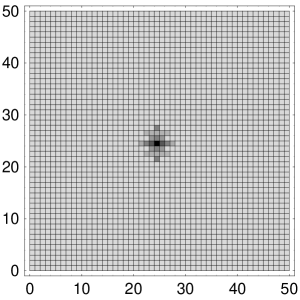
Figure 11. Risks associated with cells

Assume that the device is represented by $50\times 50=2500$ cells each of which corresponds to a possible state of the device. Each state is determined by a fixed real number $0\leq R\leq 1$ which is identified as a scaled risk of the state. According to this, every cell is characterized by a risk value. The operation of the device consists of a random selection of one cell the $R$ value of which defines the output variable $y$. The run of the ”code” corresponding to the best estimate method in this gedanken experiment means the realization of this operation. Repeating the run $N$-times, we obtain a sample with $N$ elements.

If $R=0$, then the state is safe, there is no limit violation. We suggest to investigate a device where the limit violation may occur only in a small fraction of the states, actually in 1% of the states. To simplify the presentation, the $R$ values are given in Figure 11.

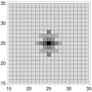
Figure 12. Central part of Fig. 11.

Most of the cells has no limit violation (light cells). Limit violation is observed only at a few cells (25 of them, 1 % of the states): 12 cells have minor limit violations ($R\leq 0.1$), their partition: $R=0.08$ in 4 cells, $R=0.09$ in 4 cells, $R=0.1$ in 4 cells. Further 10 cells have moderate limit violation ($0.1\leq R\leq 0.2$). Their partition is $R=0.15$ in 4 cells, $R=0.2$ in 6 cells, and 3 have severe limit violations ($>0.25$), their partition is $R=0.3$ in 2 cells, and $R=0.5$ in 1 cell. All the cells with limit violation are in the center of the region shown in Fig. 11, see the enlargement in Fig. 12.

The $0.95|0.95$ methodology is performed in the following way: one generates $N=59$ random integers from the set of uniformly distributed integers $1,2,\ldots,2500$, and then reads the risk values $R$ of the generated $59$ cells.  These risk values form the basic sample. The maximal element $R_{1}(59)$ of the sample defines the random interval $[0,\,R_{1}(59)]$ which covers the $95$ % of the risk distribution with probability $\beta=0.95$. Let us repeat this procedure $n=100$ times, and determine the numbers of occurrences of the risk values $0,0.08,0.09,0.1,0.15,0.2,0.3,0.5$. In order to see the effect of the strengthening requirements, we performed the same calculations in the cases of $N=90$ and $N=459$, which sample sizes correspond to the levels $0.95|0.99$ and the $0.99|0.99$, respectively.

Table 4. Maximum values of $R$ in $n=100$ calculations with sample sizes $N=59,90,458$ in each calculation.

	Number in 100 cases with
$R$	$N=59$	$N=90$	$N=458$
0.50	5	2	27
0.30	2	7	17
0.20	15	16	33
0.15	4	13	12
0.10	7	4	7
0.09	4	7	2
0.08	8	6	1
0.00	55	45	1

Actual results are given in Table 4. If $N=59$, then in 55% of the cases, we conclude (falsely) that the system is safe, and only in 7% of the samples we get an alarming large, $R>0.2$ value, from which the correct maximum is obtained in 5% of the cases. If $N=90$, then we see some moderate improvement: solely 45% of the cases show no limit violation and 9% indicate alarming limit violation. With $N=458$, only 1% of the cases show the system to be safe and 44% of the cases indicate alarmingly high limit violation.

We admit that the presented gedanken experiment is a real challenge since only one state out of 100 has appreciable limit violation, but perhaps in a real safety analysis we encounter possible device states which are safe in general except for a small fraction of the possible states. Safety analysis is done to reveal such situations. The above given considerations may give us an impression what the ”high probability” might be in 10CFR 50.46.

The reader may think that this is an exceptional case. However, it is fairly common that only a small fraction of the reasonable inputs may lead to safety hazard. Another problem is, that if we have a large number of unsafe cells, in the average, one out of 20 will remain uncovered, this is the meaning of the 95% confidence level.

6. Concluding remarks

In the validation and verification process of a code one carries out a series of computations. The input data are not precisely determined because measured data have an error, calculated data are often obtained from a more or less accurate model. Some users of large codes are content with comparing the nominal output obtained from the nominal input, whereas all the possible inputs should be taken into account when judging safety. At the same time, any statement concerning safety must be aleatory, and its merit can be judged only when the probability is known with which the statement is true.

There are several statistical tools applicable in safety analysis. Before choosing the appropriate statistical method, one has to look at the physical model. If we assume a situation where most of the possible states are safe and our task is to pinpoint the low number of possible dangerous states, we need a larger statistical sample, i.e. we have to carry out a larger number of calculations with the computer model.

On the other hand, if there are many risky states, the tolerance interval may not reveal all of them, there is a good chance that every 20th risky cell remains undetected when the tolerance level is 0.95.

The authors arrived at conclusion that the random character of the computed output values is usually neglected by the analysts. For instance, the trivial fact that the maximal value of an output variable obtained by the tolerance interval method is not repeatable, since it is a random variable, is almost forgotten in the applied uncertainty analysis. It may happen that the authority will carry out an independent safety analysis which may lead to a smaller safety reserve in 50% of the cases and the analyst may find himself/herself in an inconvenient situation. When the output variables are correlated, then the separate analysis of the variables may result incorrect statements.

Consequent application of order statistics or the application of the sign test may offer a way out of the present situation. The authors are also convinced that efforts should be made

• to study the statistics of the output variables,

• to study the occurrence of large fluctuations in the analyzed cases

• to avoid random quantities acquiring essential role in safety analysis.

All these observations should influence, in safety analysis, the application of best estimate methods, and underline the opinion that any realistic modeling and simulation of complex systems must include the probabilistic features of the system and the environment.

References

- [1] Krzykacz B, A Computer Program for the Derivation of Empirical Uncertainty Statements of Results from Large Computer Models, Report GRS-A-1720, Garching, (1990).
- [2] Clopper CJ, Pearson ES, Biometrica, 26, 404 (1934).
- [3] Brown LD, Cai TT, DasGupta A, Statistical Science, 16, 101 (2001).
- [4] Guba A, Makai M, Pál L, Rel. Eng. and System Safety, 80, 217 (2003).
- [5] Makai M, Pál L, Rel. Eng. and System Safety, 91, 222 (2006).
- [6] Kendal M, Stuart A, The advanced theory of statistics, vol. 2. London:Griffin, (1979).
- [7] Wilson EB, J. Amer. Statist. Assoc., 22, 209 (1927).
- [8] Van Der Warden BK, Mathematische Statistik, Springer Verlag (1957).
- [9] Rao CR, Linear Statistical Inference and Its Applications, Wiley, New York (1973).
- [10] Cox DR, Snell EJ, Analysis of Bynary Data, 2end ed. Chapman and Hall, London, (1989).
- [11] Newcombbe RG, Statistics in Medicine, 17, 857 (1998).