Optimal discriminating designs for several competing regression models

Abstract

The problem of constructing optimal discriminating designs for a class of regression models is considered. We investigate a version of the $T_{p}$-optimality criterion as introduced by Atkinson and Fedorov [Biometrika 62 (1975a) 289–303]. The numerical construction of optimal designs is very hard and challenging, if the number of pairwise comparisons is larger than 2. It is demonstrated that optimal designs with respect to this type of criteria can be obtained by solving (nonlinear) vector-valued approximation problems. We use a characterization of the best approximations to develop an efficient algorithm for the determination of the optimal discriminating designs. The new procedure is compared with the currently available methods in several numerical examples, and we demonstrate that the new method can find optimal discriminating designs in situations where the currently available procedures fail.

T1Supported in part by the Collaborative Research Center “Statistical modeling of nonlinear dynamic processes” (SFB 823, Teilprojekt C2) of the German Research Foundation (DFG).

and

1 Introduction

An important problem in optimal design theory is the construction of efficient designs for model identification in a nonlinear relation of the form

$$Y=\eta(x,\theta)+\varepsilon.$$ (1)

In many cases there exist several plausible models which may be appropriate for a fit to the given data. A typical example are dose-finding studies, where various models have been developed for describing the dose–response relation [Pinheiro, Bretz and Branson (2006)]. Some of these models, which have also been discussed by Bretz, Pinheiro and Branson (2005), are listed in Table 1. In these and similar situations the first step of the data analysis consists of the identification of an appropriate model from a given class of competing regression models.

The optimal design problem for model identification has a long history. Early work can be found in Stigler (1971), who determined designs for discriminating between two nested univariate polynomials by minimizing the volume of the confidence ellipsoid for the parameters corresponding to the extension of the smaller model. Several authors have worked on this approach in various other classes of nested models [Dette and Haller (1998) or Song and Wong (1999) among others].

Table 1: Candidate dose response models as a function of dose $x$

Model	Full model specification
Linear	$\eta_{1}(x,\rho_{(1)})=60+0.56x$
Quadratic	$\eta_{2}(x,\rho_{(2)})=60+(7/2250)x(600-x)$
Emax	$\eta_{3}(x,\rho_{(3)})=60+294x/(25+x)$
Logistic	$\eta_{4}(x,\rho_{(5)})=49.62+290.51/\{1+\exp[(150-x)/45.51]\}$

In a pioneering paper, Atkinson and Fedorov (1975b) proposed the $T$-optimality criterion to construct designs for discriminating between two competing regression models. It provides a design such that the sum of squares for a lack of fit test is large. Atkinson and Fedorov (1975a) extended this approach later for discriminating a selected model $\eta_{1}$ from a class of other regression models, say $\{\eta_{2},\ldots,\eta_{k}\}$, $k\geq 2$. This concept does not require competing nested models and has found considerable attention in the statistical literature; see, for example, Fedorov (1980), Fedorov and Khabarov (1986) for early and Uciński and Bogacka (2005), López-Fidalgo, Tommasi and Trandafir (2007), Atkinson (2008a, 2008b), Tommasi (2009), Wiens (2009) or Dette, Melas and Shpilev (2012) for some more recent references.

In general, the problem of finding $T$-optimal designs, either analytically or numerically, is a very hard and challenging one. Although Atkinson and Fedorov (1975b) indicated some arguments for the convergence of their iterative procedure, there is no evidence that the convergence is sufficiently fast in cases with more than two pairwise comparisons of regression models such that the procedure can be used in those applications.

In the present paper we construct optimal discriminating designs for several competing regression models where none of the models is selected in advance to be tested against all other ones. Let $d$ denote the number of pairwise comparison of interest. In Section 2 we introduce a $T_{p}$-optimality criterion, which is a weighted average of $d$ different $T$-optimality criteria corresponding to these pairs. It is demonstrated in Section 3 that the corresponding optimal design problems are closely related to (nonlinear) vector-valued approximation problems. The support points of optimal discriminating designs are contained in the set of extreme points of a best approximation, and the optimal design can be determined with the knowledge of these points. Because we are only aware of the work of Brosowski (1968) on vector-valued approximation, we consider this problem in Section 4.

Duality theory is then used to determine not only the points of the support, but also the masses. The theory shows that there exist optimal designs with a support of at most $n+1$ points, where $n$ is the total number of parameters in the competing regression models. We will illustrate by a simple example that the number of support points is usually much smaller. It turns out that this fact occurs in particular for $d\geq 3$ comparisons, and therefore our investigations explain the difficulties in the computation of $T$-optimal discriminating designs. For this reason we find numerical results in the literature mainly for the cases $d=1$ and $d=2$, and advanced techniques are required for the determination of $T_{p}$-optimal discriminating designs if $d\geq 3$.

In Sections 5 and 6 we use the theoretical results to develop an efficient algorithm for calculating $T_{p}$-optimal discriminating designs. The main idea of the algorithm is very simple and essentially consists of two steps. [(1)]

The relation to the corresponding vector-valued approximation problem is used to identify a reference set which contains all support of the $T_{p}$-optimal discriminating design. This is done by linearizing the optimization problem. A combinatorial argument in connection with dual linear programs determines which points are included in the support of the optimal design.

A linearization of a saddle point problem that is concealed behind the design problem is used for a simultaneous update of all weights. The implementation of these two steps which are usually iterated is more complicated and described in Section 6. Some comments regarding the convergence and details for the main technical step of the algorithm are given in the supplementary material [Braess and Dette (2013)] to this paper. In Section 7 we provide several numerical examples and compare our approach with the currently available methods. In particular, we consider the problem of determining optimal discriminating designs for the dose response models specified in Table 1. Here the currently available procedure fails in the case of many pairwise comparisons, while the new method determines a design with high efficiency in less than $10$ iteration steps.

2 Preliminaries

Following Kiefer (1974) we consider designs that are defined as probability measures with finite support on a compact design space $\mathcal{X}$. If the design $\xi$ has masses $w_{1},\ldots,w_{\nu}$ at the distinct points $x_{1},\ldots,x_{\nu}$, then observations are taken at these points with the relative proportions given by the masses. Let $\mathcal{M}=\{\eta_{1},\ldots,\eta_{k}\}$ denote a class of possible models for the regression function $\eta$ in (1), where $\theta_{(j)}$ denotes the vector of parameters in model $\eta_{j}$ that varies in the set $\Theta^{(j)}$ $(j=1,\ldots,k)$. Atkinson and Fedorov (1975a) proposed to select one model in $\mathcal{M}$, say $\eta_{1}$, to fix its vector of parameters $\rho_{(1)}$ and to determine a discriminating design by maximizing

$$\min_{2\leq j\leq k}T_{1,j}(\xi),$$ (2)

where

$$T_{1,j}(\xi):=\inf_{\theta_{(j)}\in\Theta^{(j)}}\int_{\mathcal{X}}\bigl{[}\eta_{1}(x,\rho_{(1)})-\eta_{j}(x,\theta_{(j)})\bigr{]}^{2}\,d\xi(x)\qquad(2\leq j\leq k).$$

If the competing regression models $\eta_{1},\ldots,\eta_{k}$ are not nested (as in Table 1), it is not clear which model should be fixed in this approach, and it is useful to have more “symmetry” in this concept. For illustration consider the case of two competing nonnested models, say $\eta_{i}(x,\theta_{(i)}),\eta_{j}(x,\theta_{(j)})$, and assume that the experimenter can fix a parameter for each model, say $\rho_{(1)}$ and $\rho_{(2)}$. In this case for a given design $\xi$ there exist two $T$-optimality criteria, say $T_{1,2}$ and $T_{2,1}$, corresponding to the specification of the model $\eta_{1}$ or $\eta_{2}$, respectively, where

$$T_{i,j}(\xi) := \inf_{\theta_{(j)}\in\Theta^{(j)}}\Delta_{i,j}(\theta_{(j)},\xi)$$

$$\phantom{:}= \inf_{\theta_{(j)}\in\Theta^{(j)}}\int_{\mathcal{X}}\bigl{[}\eta_{i}(x,\rho_{(i)})-\eta_{j}(x,\theta_{(j)})\bigr{]}^{2}\,d\xi(x)$$

$(i\neq j)$. The first index $i$ in the term $\Delta_{i,j}$ corresponds to the fixed model $\eta_{i}(x,\rho_{(i)})$, while the minimum in (2) is taken with respect to the parameter of the model specified by the index $j$. The parameter associated to the minimum is denoted as

$$\theta^{*}_{(i,j)}:=\mathop{\operatorname{argmin}}_{\theta_{(j)}\in\Theta^{(j)}}\Delta_{i,j}(\theta_{(j)},\xi),$$ (4)

where we assume its existence and do not reflect its dependence on the design $\xi$ and the parameter $\rho_{(i)}$ since this will always be clear from the context. Note that we use the notation $\theta_{(i,j)}^{*}$ for the parameter corresponding to the best approximation of the model $\eta_{i}$ (with fixed paramater $\rho_{(i)}$) by the model $\eta_{j}$.

If a discriminating design has to be constructed for $k$ competing models, there exist $k(k-1)$ expressions of the form (2). Let $p_{i,j}$ be given nonnegative weights satisfying $\sum_{i\neq j}p_{i,j}=1$, then a design $\xi^{*}$ is called $T_{p}$-optimal discriminating for the class of models $\mathcal{M}=\{\eta_{1},\ldots,\eta_{k}\}$ if it maximizes the functional

$$T(\xi):=\sum_{1\leq i\neq j\leq k}p_{i,j}T_{i,j}(\xi)=\sum_{1\leq i\neq j\leq k}p_{i,j}\inf_{\theta_{(j)}\in\Theta^{(j)}}\Delta_{i,j}(\theta_{(j)},\xi)$$ (5)

[see also Atkinson and Fedorov (1975a)]. Note that the special choice $p_{i,j}>0$ $(j=2,\ldots,k)$, $p_{i,j}=0$ $(i=2,\ldots,k,$ $j=2,\ldots,k;i\neq j)$, refers to the case where one model (namely $\eta_{1}$) has been fixed and is tested against all other ones. The criterion (5) provides a more symmetric formulation of the general discriminating design problem. It has also been investigated by Tommasi and López-Fidalgo (2010) among others for $k=2$ competing regression models. They proposed to maximize a weighted mean of efficiencies which is equivalent to the criterion (5) if the weights $p_{i,j}$ are chosen appropriately.

In order to deal with the general case we denote the set of indices corresponding to the positive weights in (5) as

$$\mathcal{I}:=\bigl{\{}(i,j)\mid p_{i,j}>0;1\leq i\neq j\leq k\bigr{\}}.$$

We assume without loss of generality that the set $\mathcal{I}$ can be decomposed in $p\leq k$ subsets of the form $\{(i,j)\in\mathcal{I}\mid 1\leq j\leq k\}$ and define $\mathcal{I}_{i}=\{j\in\{1,\ldots,k\}\mid(i,j)\in\mathcal{I}\}$ as the set of indices corresponding to those models which are used for a comparison with model $\eta_{i}$. For each model $\eta_{i}$ $(i=1,2,\ldots,p)$, a parameter, say $\rho_{(i)}$, is fixed due to prior information, and the model $\eta_{i}(x,\rho_{(i)})$ has to be discriminated from the other ones in the set $\mathcal{I}_{i}$. Define

$$\lambda_{i}:=\#\mathcal{I}_{i},\qquad d:=\sum^{p}_{i=1}\lambda_{i}$$ (6)

as the cardinality of the sets $\mathcal{I}_{i}$ and $\mathcal{I}$, respectively. Note that $d$ denotes the total number of pairwise comparisons included in the optimality criterion (5). Consider the space $\mathcal{F}_{d}=C(\mathcal{X})^{d}$ of continuous vector-valued functions defined on $\mathcal{X}$, and define for a function $g=(g_{ij})_{(i,j)\in\mathcal{I}}\in\mathcal{F}_{d}$ a norm by

$$\|g\|:=\sup_{x\in\mathcal{X}}\bigl{|}g(x)\bigr{|},$$ (7)

where $|g(x)|^{2}:=\sum_{(i,j)\in\mathcal{I}}p_{i,j}g^{2}_{ij}(x)$ denotes a weighted Euclidean norm on $\mathbb{R}^{d}$. In this framework the distance between two functions $f,g\in\mathcal{F}_{d}$ is given by $\|f-g\|$. Next, given the parameters $\rho_{(1)},\ldots,\rho_{(p)}$ for the models $\eta_{1},\ldots,\eta_{p}$, respectively, due to prior information, define the $d$-dimensional vector-valued function

$$\qquad\eta(x):=\bigl{(}\underbrace{\eta_{1}(x,\rho_{(1)}),\ldots,\eta_{1}(x,\rho_{(1)})}_{\lambda_{1}\ \mathrm{times}},\ldots,\underbrace{\eta_{p}(x,\rho_{(p)}),\ldots,\eta_{p}(x,\rho_{(p)})}_{\lambda_{p}\ \mathrm{times}}\bigr{)}^{T},$$ (8)

where each function $\eta_{j}(x,\rho_{(j)})$ appears $\lambda_{j}$ times in the vector $\eta(x)$. We also consider a vector of approximating functions

$$\qquad\eta(x,\theta):=\bigl{(}\underbrace{\bigl{(}\eta_{j}(x,\theta_{(1,j)})\bigr{)}_{j\in\mathcal{I}_{1}}}_{\in\mathbb{R}^{\lambda_{1}}},\ldots,\underbrace{\bigl{(}\eta_{j}(x,\theta_{(p,j)})\bigr{)}_{j\in\mathcal{I}_{p}}}_{\in\mathbb{R}^{\lambda_{p}}}\bigr{)}^{T}\in\mathcal{F}_{d}.$$ (9)

We emphasize again that we use the notation $\theta_{(i,j)}$ for the parameter in the model $\eta_{j}$. This means that different parameters $\theta_{(i,j)}$ and $\theta_{(k,j)}$ are used if the model $\eta_{j}$ has to be discriminated from the models $\eta_{i}$ and $\eta_{k}$ ($i\neq k$). The corresponding parameters are collected in the vector

$$\qquad\theta=\bigl{(}(\theta_{(1,j)})_{j\in\mathcal{I}_{1}},\ldots,(\theta_{(p,j)})_{j\in\mathcal{I}_{p}}\bigr{)}^{T}\in\Theta=\bigotimes^{p}_{i=1}\bigotimes_{j\in\mathcal{I}_{i}}\Theta^{(j)},$$ (10)

and we denote by $n:=\dim\Theta=\sum^{p}_{i=1}\sum_{j\in\mathcal{I}_{i}}\dim\Theta^{(j)}$ the total number of all parameters involved in the $T_{p}$-optimal discriminating design problem. With this notation the optimal design problem can be rewritten as

$$\max_{\xi}\sum_{1\leq i\neq j\leq p}p_{i,j}\min_{\theta_{(j)}\in\Theta^{(j)}}\Delta_{i,j}(\theta_{(j)},\xi),$$ (11)

and the following examples illustrate this general setting.

Example 2.1.

Consider the case $k=3$ and assume that all weights $p_{i,j}$ in the criterion (5) are positive. Here no model is preferred, and there are $6$ pairwise comparisons. This yields $p=k=3$,

$$\mathcal{I} = \bigl{\{}(1,2),(1,3),(2,1),(2,3),(3,1),(3,2)\bigr{\}},$$

$$\mathcal{I}_{1} = \{2,3\},\qquad\mathcal{I}_{2}=\{1,3\},\qquad\mathcal{I}_{3}=\{1,2\},$$

$\lambda_{1}=\lambda_{2}=\lambda_{3}=2$ and $d=6$. We obtain for the vectors in (8) and (9)

$$\eta(x) = \bigl{(}\eta_{1}(x,\rho_{(1)}),\eta_{1}(x,\rho_{(1)}),\eta_{2}(x,\rho_{(2)}),\eta_{2}(x,\rho_{(2)}),$$

$$\hskip 112.0pt\eta_{3}(x,\rho_{(3)}),\eta_{3}(x,\rho_{(3)})\bigr{)}^{T},$$

$$\eta(x,\theta) = \bigl{(}\eta_{2}(x,\theta_{(1,2)}),\eta_{3}(x,\theta_{(1,3)}),\eta_{1}(x,\theta_{(2,1)}),\eta_{3}(x,\theta_{(2,3)}),$$

$$\hskip 124.0pt\eta_{1}(x,\theta_{(3,1)}),\eta_{2}(x,\theta_{(3,2)})\bigr{)}^{T},$$

with

$$\theta = (\theta_{(1,2)},\theta_{(1,3)},\theta_{(2,1)},\theta_{(2,3)},\theta_{(3,1)},\theta_{(3,2)})^{T}$$

$$\in \Theta^{(2)}\times\Theta^{(3)}\times\Theta^{(1)}\times\Theta^{(3)}\times\Theta^{(1)}\times\Theta^{(2)}.$$

Example 2.2.

Consider the problem of discriminating between $k=3$ nested polynomial models $\eta_{1}(x,\theta_{(1)})=\theta_{10}+\theta_{11}x$, $\eta_{2}(x,\theta_{(2)})=\theta_{20}+\theta_{21}x+\theta_{22}x^{2}$ and $\eta_{3}(x,\theta_{(3)})=\theta_{30}+\theta_{31}x+\theta_{32}x^{2}+\theta_{33}x^{3}$. A common strategy to identify the degree of the polynomial is to test a quadratic against a linear and a cubic against the quadratic model. In this case we choose only two positive weights $p_{2,1}$ and $p_{3,2}$ in the criterion (5) which yields $\mathcal{I}=\{(2,1),(3,2)\},$ $\mathcal{I}_{1}=\{1\},$ $\mathcal{I}_{2}=\{2\},$ $p=2$, $\lambda_{1}=\lambda_{2}=1$ and $d=2$. The functions $\eta$ and $\eta(\cdot,\theta)$ are given by $\eta(x)=(\eta_{2}(x,\rho_{(2)}),\eta_{3}(x,\rho_{(3)}))^{T},$

$$\eta(x,\theta) = \bigl{(}\eta_{1}(x,\theta_{(2,1)}),\eta_{2}(x,\theta_{(3,2)})\bigr{)}^{T}=\bigl{(}\theta_{10}+\theta_{11}x,\theta_{20}+\theta_{21}x+\theta_{22}x^{2}\bigr{)}^{T},$$

respectively, where $\theta=(\theta_{(2,1)},\theta_{(3,2)})^{T}\in\mathbb{R}^{5}.$

3 Characterization of optimal designs

The $T_{p}$-optimality of a given design $\xi$ can be checked by an equivalence theorem (Theorem 3.1) that can be proved by the same arguments as used by Atkinson and Fedorov (1975a). As usual, the following properties tacitly are assumed to hold: [(A1)]

The regression functions $\eta_{i}(x,\theta_{(i)})$ are differentiable with respect to the parameter $\theta_{(i)}$ ($i=1,\ldots,k$).

Let $\xi^{*}$ be a $T_{p}$-optimal discriminating design. The parameter $\theta^{*}=(\theta^{*}_{(i,j)})^{T}_{(i,j)\in\mathcal{I}}$ defined by (4) exists, is unique and an interior point of $\Theta$. Both assumptions are always satisfied in linear models. Moreover, assumption (A1) is satisfied for many commonly used nonlinear regression models; see Seber and Wild (1989). It is usually harder to check assumption (A2) because it depends on the individual $T_{p}$-optimal design.

Theorem 3.1 ((Equivalence theorem))

A design $\xi$ is a $T_{p}$-optimal discriminating design for the class of models $\mathcal{M}$ if and only if for all $x\in\mathcal{X}$,

$$\psi(x,\xi):=\sum_{(i,j)\in\mathcal{I}}p_{i,j}\bigl{[}\eta_{i}(x,\rho_{i})-\eta_{j}\bigl{(}x,\theta_{(i,j)}^{*}\bigr{)}\bigr{]}^{2}\leq T(\xi),$$ (12)

where $\theta^{*}_{(i,j)}$ is defined by (4). Moreover, if $\xi$ is a $T_{p}$-optimal discriminating design, then equality holds in (12) for all support points of $\xi$.

The equivalence theorem asserts that there is no gap between the solution of the max min problem (11) and the corresponding min max problem. The following result shows that the $T_{p}$-optimal design problem is intimately related to a nonlinear vector-valued approximation problem with respect to the norm (7).

Theorem 3.2

Let $\eta$, $\eta(\cdot,\theta)$ and $T(\xi)$ be defined by (9), (10) and (5), respectively, then

$$\sup_{\xi}T(\xi)=\inf_{\theta\in\Theta}\bigl{\|}\eta-\eta(\cdot,\theta)\bigr{\|}^{2},$$ (13)

that is, with $\psi$ defined in the equivalence theorem

$$\sup_{\xi}\inf_{\theta\in\Theta}\int_{\mathcal{X}}\psi(x,\xi)\,d\xi=\inf_{\theta\in\Theta}\sup_{\xi}\int_{\mathcal{X}}\psi(x,\xi)\,d\xi.$$ (14)

If $\xi^{*}$ maximizes $T(\xi)$, then the vector $\theta^{*}=(\theta^{*}_{(i,j)})_{(i,j)\in\mathcal{I}}$ defined in (4) satisfies

$$\bigl{\|}\eta(x)-\eta\bigl{(}x,\theta^{*}\bigr{)}\bigr{\|}=\inf_{\theta\in\Theta}\bigl{\|}\eta(x)-\eta(x,\theta)\bigr{\|}=T\bigl{(}\xi^{*}\bigr{)}.$$ (15)

Moreover, the support of the $T_{p}$-optimal discriminating design $\xi^{*}$ for the class $\mathcal{M}$ satisfies

$$\operatorname{supp}\bigl{(}\xi^{*}\bigr{)}\subset\mathcal{A}:=\bigl{\{}x\in\mathcal{X}|\bigl{|}\eta(x)-\eta\bigl{(}x,\theta^{*}\bigr{)}\bigr{|}=\bigl{\|}\eta-\eta\bigl{(}\cdot,\theta^{*}\bigr{)}\bigr{\|}\bigr{\}}.$$ (16)

We have for any design $\tilde{\xi}$ the relation

$$\inf_{\theta\in\Theta}\int_{\mathcal{X}}\psi(x,\xi)\,d\tilde{\xi}\leq\inf_{\theta\in\Theta}\sup_{\xi}\int_{\mathcal{X}}\psi(x,\xi)\,d\xi,$$

and the left-hand side of (14) cannot be larger than the right-hand side, that is, $T(\tilde{\xi})\leq\inf_{\theta\in\Theta}\|\eta-\eta(\cdot,\theta)\|^{2}$. Since $\tilde{\xi}$ is an arbitrary design, the bound holds also for $\sup_{\xi}T(\xi)$. This means in terms of (13) $\sup_{\xi}T(\xi)\leq\inf_{\theta\in\Theta}\|\eta-\eta(\cdot,\theta)\|^{2}$.

Now the characterization of $T_{p}$-optimality in Theorem 3.1 and the definition of $\theta^{*}=(\theta^{*}_{(i,j)})_{(i,j)\in\mathcal{I}}$ in Theorem 3.1 yield

$$T\bigl{(}\xi^{*}\bigr{)} \leq \inf_{\theta\in\Theta}\bigl{\|}\eta-\eta(\cdot,\theta)\bigr{\|}^{2}\leq\bigl{\|}\eta-\eta\bigl{(}\cdot,\theta^{*}\bigr{)}\bigr{\|}^{2}$$

$$= \sup_{x\in\mathcal{X}}\sum_{(i,j)\in\mathcal{I}}p_{i,j}\bigl{[}\eta_{i}(x,\rho_{(i)})-\eta_{j}\bigl{(}x,\theta^{*}_{(i,j)}\bigr{)}\bigr{]}^{2}\leq T\bigl{(}\xi^{*}\bigr{)},$$

which proves the first part of Theorem 3.2. The statement on the support points of $\xi^{*}$ follows directly from these considerations.

Equality (15) means that the parameter $\theta^{*}$ defined in (4) corresponds to the best approximation of the function $\eta$ in (8) by functions of the form (9) with respect to the norm (7). If this nonlinear approximation problem has been solved, and the parameter $\bar{\theta}=((\bar{\theta}_{(i,j)})_{j\in\mathcal{I}_{1}},\ldots,(\bar{\theta}_{(p,j)})_{j\in\mathcal{I}_{p}})$ corresponds to a best approximation, that is,

$$\bigl{\|}\eta-\eta(\cdot,\bar{\theta})\bigr{\|}^{2}=\min_{\theta\in\Theta}\bigl{\|}\eta-\eta(\cdot,\theta)\bigr{\|}^{2},$$ (17)

it follows from Theorem 3.2 that the support of the $T_{p}$-optimal discriminating design is contained in the set $\mathcal{A}$ defined in (16). In linear models and in many of the commonly used nonlinear regression models $\theta^{*}$ and $\bar{\theta}$ are uniquely determined.

Example 3.3.

In Example 2.1 we considered discriminating design problems for 3 rival models $\eta_{1},\eta_{2},\eta_{3}$ and all weights in the optimality criterion are positive. By Theorem 3.2 the support of the $T_{p}$-optimal discriminating design problem can be found by solving the nonlinear vector-valued approximation problem

$$\inf_{\theta\in\Theta}\bigl{\|}\eta-\eta(\cdot,\theta)\bigr{\|}^{2}=\inf\biggl{\{}\sup_{x\in\mathcal{X}}\sum_{1\leq i\neq j\leq 3}p_{i,j}\bigl{|}\eta_{i}(x,\rho_{(i)})-\eta_{j}(x,\theta_{(i,j)})\bigr{|}^{2}\Big{|}$$

$$\hskip 187.0pt\theta_{(i,j)}\in\Theta^{(j)};1\leq i\neq j\leq 3\biggr{\}}.$$

The following result is an approach in this framework for the calculation of the masses of the $T_{p}$-optimal discriminating design.

Corollary 3.4

Assume that a parameter $\bar{\theta}$ defined in (17) exists and is an interior point of $\Theta$, and let $\nabla_{\theta_{(i,j)}}$ denote the gradient of $\eta_{j}$ with respect to $\theta_{(i,j)}$. [(a)]

If a design $\xi$ is a $T_{p}$-optimal discriminating design for the class $\mathcal{M}$, then

$$\int_{\mathcal{A}}\bigl{(}\eta_{i}(x,\rho_{(i)})-\eta_{j}(x,\bar{\theta}_{(i,j)})\bigr{)}\nabla_{\theta_{(i,j)}}\eta_{j}(x,\theta_{(i,j)})|_{\theta_{(i,j)}=\bar{\theta}_{(i,j)}}\,d\xi(x)=0$$ (18)

holds for all $(i,j)\in\mathcal{I}$.

Conversely, if all competing models are linear, and the design $\xi$ satisfies (18) such that $\operatorname{supp}(\xi)\subset\mathcal{A}$, then $\xi$ is a $T_{p}$-optimal discriminating design for the class $\mathcal{M}$.

If condition (18) is not satisfied, there is a direction in the parameter space $\Theta$ in which the criterion decreases. Thus (18) is a necessary condition. From Theorem 3.2 we know that the best approximation gives rise to a $T_{p}$-optimal design, and it follows from a uniqueness argument that the condition is also sufficient in this case.

4 Chebyshev approximation of $d$-variate functions

By Theorem 3.2, a $T_{p}$-optimal discriminating design is associated to an approximation problem in the space of continuous $d$-variate functions on the compact design space $\mathcal{X}$ where $d$ is the number of comparisons as specified by (6). This relation can be used for the computation of $T_{p}$-optimal designs and for the evaluation of the efficiency of computed designs.

In this section we will investigate these approximation problems in more detail for the case of linear models. We restrict the presentation to linear models because we want to emphasize that the main difficulties already appear in linear models if $d\geq 3$. The extension to nonlinear regression models is straightforward and will be provided in Section 6.3.

The general theory here and in the previous section provides only the information that a $T_{p}$-optimal discriminating design exists with $n+1$ or less support points where $n=\dim\Theta$. We will demonstrate in Section 4.2 that the number of support points is often much smaller than $n+1$. This is the reason for the difficulties in the numerical construction, even if only linear models are involved. In contrast to other methods [see, e.g., López-Fidalgo, Tommasi and Trandafir (2007)] the construction via the approximation problem has the advantage that the points of the support of the $T_{p}$-optimal discriminating design are directly calculated.

4.1 Characterization of best approximations

We will avoid double indices for vectors and vector-valued functions throughout this section in order to avoid confusion with matrices. We write $\theta=(\theta_{1},\theta_{2},\ldots,\theta_{n})^{T}$ instead of $(\theta_{(i,j)})^{T}_{(i,j)\in\mathcal{I}}$ and $(f_{1},\ldots,f_{d})^{T}$ instead of the vector $\eta(x)$ defined in (8). The approximation problem is considered for a given $d$-variate function $f=(f_{1},\ldots,f_{d})^{T}\in\mathcal{F}_{d}=C(\mathcal{X})^{d}$. It is not necessary that some components of $f$ are equal as it occurs in the function (8).

In the case of linear models, equation (9) defines an $n$-dimensional linear subspace

$$V=\Biggl{\{}v=\sum_{m=1}^{n}\theta_{m}v_{m}\bigg{|}\theta=(\theta_{1},\theta_{2},\ldots,\theta_{n})\in\mathbb{R}^{n}\Biggr{\}}\subset\mathcal{F}_{d},$$ (19)

where $v_{1},v_{2},\ldots,v_{n}\in\mathcal{F}_{d}$ denotes a basis of $V$, and $n$ is the dimension of the parameter space $\Theta$ in (10). Note that $f(x)$ and $v(x)$ are $d$-dimensional vectors for $x\in\mathcal{X}$ and $v\in V$. Theorem 3.2 relates the $T_{p}$-optimal discriminating design problem to the problem of determining the best Chebyshev approximation $u^{*}$ of the function $f$ by elements of the subspace $V$, that is,

$$\bigl{\|}f-u^{*}\bigr{\|}=\min_{v\in V}\|f-v\|.$$

As stated in (7), the norm $\|\cdot\|$ refers to the maximum-norm on $C(\mathcal{X})^{d}$, $\|g\|:=\sup_{x\in\mathcal{X}}|g(x)|$, where the weighted Euclidean norm $|\cdot|$ and the corresponding inner product in $\mathbb{R}^{d}$ are defined by

$$|r|^{2}:=\sum_{l=1}^{d}p_{l}|r_{l}|^{2},\qquad\langle\tilde{r},r\rangle:=\sum_{l=1}^{d}p_{l}\tilde{r}_{l}r_{l},\qquad r,\tilde{r}\in\mathbb{R}^{d}$$ (20)

[here the weights $p_{l}$ correspond to the weights $p_{i,j}$ used in the definition (7)]. Because the family $V$ defined in (19) is a linear space, the classical Kolmogorov criterion [see Meinardus (1967)] can be generalized to the problem of vector-valued approximation. The result is easily obtained from the cited literature if products of real or complex numbers in the proof of the classical theorem are replaced by the Euclidean inner products of $d$-vectors. The nonlinear character of the procedures for determining best approximations does not matter at this point.

Lemma 4.1 ((Kolmogorov criterion for vector-valued approximation))

Let $u\in V$ and

$$\mathcal{A}:=\bigl{\{}x\in\mathcal{X}|\bigl{|}\varepsilon(x)\bigr{|}=\|\varepsilon\|\bigr{\}}$$ (21)

be the set of extreme points of the error function $\varepsilon:=f-u.$ The $d$-variate function $u$ is a best approximation to $f$ in $V$ if and only if for all $v\in V$,

$$\min_{x\in\mathcal{A}}\bigl{\langle}\varepsilon(x),v(x)\bigr{\rangle}\leq 0.$$ (22)

Assume that $u$ is a best approximation of the function $f$. Condition (22) in the Kolmogorov criterion means that the system of inequalities

$$\bigl{\langle}\varepsilon(x),v_{0}(x)\bigr{\rangle}>0\qquad\forall x\in\mathcal{A}$$

is not solvable. Let $v_{1},v_{2},\ldots,v_{n}$ be a basis of $V$. Using the representation

$$v(x)=\sum_{m=1}^{n}\alpha_{m}v_{m}(x)$$ (23)

and setting $r_{m}(x):=\langle\varepsilon(x),v_{m}(x)\rangle$ we obtain the unsolvable system

$$\sum_{m=1}^{n}\alpha_{m}r_{m}(x)>0\qquad\forall x\in\mathcal{A}$$ (24)

for the vector $\alpha=(\alpha_{1},\alpha_{2},\ldots,\alpha_{n})^{T}\in\mathbb{R}^{n}$. The numbers $r_{m}(x)$ are considered as the components of a vector $r(x)$, and by the theorem on linear inequalities [see Cheney (1966), page 19] it follows that the system (24) is not solvable if and only if the origin in $\mathbb{R}^{n}$ is contained in the convex hull of the vectors $\{r(x)=(r_{1}(x),\ldots,r_{n}(x))^{T},x\in\mathcal{A}\}.$ By Carathéodory’s theorem there are $\nu\leq n+1$ points $x_{1},\ldots,x_{\nu}\in\mathcal{A}$ and numbers $w_{1},\ldots,w_{\nu}\geq 0$ such that $\sum_{i=1}^{\nu}w_{i}=1$ and

$$\sum^{\nu}_{i=1}w_{i}r(x_{i})=\sum_{i=1}^{\nu}w_{i}\bigl{\langle}\varepsilon(x_{i}),v(x_{i})\bigr{\rangle}=0\qquad\forall v\in V.$$ (25)

Theorem 4.2 ((Characterization theorem))

Let $u\in V$ and $\mathcal{A}$ be the set of extreme points of $\varepsilon=f-u$. The following statements are equivalent: [(iii)]

$u$ is a best approximation to $f$ in $V$.

There exist $\nu\leq n+1$ points $x_{1},x_{2},\ldots,x_{\nu}\in\mathcal{A}$ such that for all $v\in V$

$$\min_{1\leq i\leq\nu}\bigl{\langle}\varepsilon(x_{i}),v(x_{i})\bigr{\rangle}\leq 0.$$ (26)

There exist $\nu\leq n+1$ points $x_{1},x_{2},\ldots,x_{\nu}\in\mathcal{A}$ and $\nu$ weights $w_{1}$, $w_{2},\ldots,w_{\nu}\geq 0$, $\sum_{i=1}^{\nu}w_{i}=1$ such that the functional

$$\ell(g):=\frac{1}{\|\varepsilon\|}\sum_{i=1}^{\nu}w_{i}\bigl{\langle}\varepsilon(x_{i}),g(x_{i})\bigr{\rangle}$$ (27)

satisfies

$$\ell(\varepsilon)=\|\varepsilon\|,\qquad\|\ell\|=1\quad\mbox{and}\quad V\subset\ker(\ell),$$ (28)

where $\ker(\ell)=\{v\in V\mid\ell(v)=0\}$ denotes the kernel of the linear functional $\ell$.

The equivalence of (i) and (ii) follows from the Kolmogorov criterion. To verify the equivalence with condition (iii), let $u^{*}$ be a best approximation and $\varepsilon^{*}=f-u^{*}$. Define the functional (27) with the parameters $x_{i}$ and $w_{i}$ from (25). By the Cauchy–Schwarz inequality we obtain $\langle\varepsilon^{*}(x_{i}),g(x_{i})\rangle\leq|\varepsilon^{*}(x_{i})||g(x_{i})|\leq\|\varepsilon^{*}\|\|g\|$ with equality if $g=\varepsilon^{*}$. Since $\sum_{i}w_{i}=1$, it follows that $\ell(g)\leq\|g\|$, again with equality if $g=\varepsilon^{*}$, and the properties in (28) are verified.

Finally, assume that $u\in V$, and a functional with the properties (28) exists. We have for any $v\in V$

$$\|f-v\|=\|\ell\|\|f-v\|\geq\ell(f-v)=\ell(f-u)+\ell(u-v)=\|f-u\|+0,$$

and $u$ is a best approximation.

The extreme points $x_{1},x_{2},\ldots,x_{\nu}$ and the masses $w_{1},w_{2},\ldots,w_{\nu}$ in Theorem 4.2 define the $T_{p}$-optimal discriminating design. This follows from part (iii) of the theorem that is closely related to condition (18) in Corollary 3.4. Indeed, assume that (iii) in the theorem is satisfied, and consider a design $\xi^{*}$ with weights $w_{1},w_{2},\ldots,w_{\nu}$ at the points $x_{1},x_{2},\ldots,x_{\nu}$. It follows for all $v\in V$ that ${\|\varepsilon^{*}\|}\ell(v)=\int_{\mathcal{A}}\langle f(x)-u^{*}(x),v(x)\rangle\,d\xi^{*}(x)=0$, and by inserting the elements $v_{1},v_{2},\ldots,v_{n}$ of the basis of $V$ we obtain precisely condition (18). Consequently, there exists a $T_{p}$-optimal discriminating design with at most $n+1$ support points. As we will see in Lemma 5.3, functions satisfying only some of the properties in Theorem 4.2(iii) will also play an important role.

4.2 The number of support points—the generic case

By the characterization theorem there exists an optimal design with at most $n+1$ support points. If the number of points in the set $\mathcal{A}$ equals $n+1$, then the masses $w_{1},w_{2},\ldots,w_{n+1}$ of an optimal design can be calculated by the $n$ equations (18) together with the normalization $\int_{\mathcal{A}}\,d\xi(x)=1$. In most real-life problems, however, the number of support points is substantially smaller than $n+1$, and we obtain from (18) more equations than unknown masses. In this case the problem is ill-conditioned and the numerical computation of the masses will be more sophisticated. The following example illustrates the statement on the support.

Example 4.3.

We reconsider Example 2.2 for the polynomial regression models. The weights $p_{2,1}$ and $p_{3,2}$ are chosen as positive numbers. Since all functions are polynomials, we may assume $\mathcal{X}=[-1,+1]$ without loss of generality. A quadratic polynomial $f_{1}$ is approximated by linear polynomials in the first component, and a cubic polynomial $f_{2}$ is approximated by quadratic polynomials in the second component. Therefore, $V=\mathcal{P}_{1}\times\mathcal{P}_{2}$, where $\mathcal{P}_{k}$ denotes the set of polynomials of degree $\leq k$.

We note that the character of the approximation problem does not change if we subtract a linear polynomial from $f_{1}$ and a quadratic polynomial from $f_{2}$. Therefore we can assume that $f(x)=(\rho_{2}x^{2},\rho_{3}x^{3})^{T}$. Symmetry arguments show that the best approximating functions will be polynomials with the same symmetry, and we obtain the reduced approximation problem

$$\min_{\theta_{1},\theta_{2}\in\mathbb{R}}\sup_{x\in[-1,1]}\bigl{(}p_{2,1}\bigl{|}\rho_{2}x^{2}-\theta_{1}\bigr{|}^{2}+p_{3,2}\bigl{|}\rho_{3}x^{3}-\theta_{2}x\bigr{|}^{2}\bigr{)}.$$

We now fix the given parameters as $\rho_{2}=\rho_{3}=1$ and the weights in the $T_{p}$-optimality criterion as $p_{2,1}=p_{3,2}=1/2$. The best approximation is given by $u^{*}(x)=(1/2,x)^{T}$, that is, the first component is the best approximation of the univariate function $f_{1}$, and the second component interpolates $f_{2}$ at the extreme points of $f_{1}-u^{*}_{1}$. The function $\psi(x)=|f(x)-u^{*}(x)|^{2}=(x^{6}-x^{4}+1/4)/2$ is depicted in the left part of Figure 1. The support of the $T_{p}$-optimal discriminating design $\xi^{*}$ is a subset of the set of extreme points $\mathcal{A}=\{-1,0,+1\}$ of the function $|f-u^{*}|^{2}$. The linear functional $\ell$ in Theorem 4.2 is easily determined as $\ell(g)=\sqrt{2}[\frac{1}{4}g(-1)-\frac{1}{2}g(0)+\frac{1}{4}g(1)].$ The characterization theorem, Theorem 4.2, yields the associated $T_{p}$-optimal discriminating design

$$\xi^{*}=\pmatrix{-1&0&1\vspace*{2pt}\cr\frac{1}{4}&\frac{1}{2}&\frac{1}{4}},$$ (29)

where the first line provides the support and the second one the associated masses. The degeneracy is now obvious. The dimension of the set $V\subset\mathcal{F}_{2}$ is $n=5$, but the solution of the corresponding approximation problem has only $3$ extreme points. This degeneracy is counter intuitive. When univariate functions are approximated by polynomials in $\mathcal{P}_{2}$, then by Chebyshev’s theorem there are at least 4 extreme points. Although our approximation problem with 2-variate functions contains more functions and more parameters, the number of extreme points is smaller.

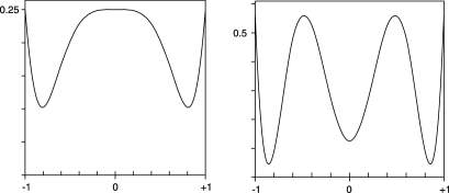
Figure 1: Error functions $\psi(x)=|f(x)-u^{*}(x)|^{2}$ in the equivalence theorem for Example 4.3. Left panel: $\rho_{2}=\rho_{3}=1$; right panel: $\rho_{2}=1,\rho_{3}=4$.

Note also that the second component is determined by interpolation and not by a direct optimization. The same designs are obtained whenever $p_{2,1}\rho_{2}^{2}\geq p_{3,2}\rho_{3}^{2}$. If this condition does not hold, we may have $4$ extreme points, as shown in the right part of Figure 1 for the choice $\rho_{2}=1;$ $\rho_{3}=4$. The solution is also degenerate. Here, the location of the support points depends on the value of $\rho_{3}$. In the mentioned case we obtain (subject to rounding) the $T_{p}$-optimal discriminating design with masses $0.18$, $0.32$, $0.32$, $0.18$ at the points $-1$, $-0.48$, $0.48$ and $1$.

The previous example shows that the cardinality of the support depends on the given parameters $\rho_{(1)},\rho_{(2)},\ldots,\rho_{(p)}$. The following definition helps one to understand which cardinality is found in most cases.

Definition 4.4.

Let $\xi^{*}$ be a $T_{p}$-optimal discriminating design for the given data $\rho_{(1)},\rho_{(2)},\ldots,\rho_{(p)}$ with $\nu\leq n+1$ support points. The design $\xi^{*}$ is called a generic point if for all parameters in some neighborhood of $\rho_{(1)},\rho_{(2)},\ldots,\rho_{(p)}$ the corresponding $T_{p}$-optimal discriminating designs have the same number $\nu$ of support points.

Our numerical experience leads to the following:

Conjecture 4.5.

If a $T_{p}$-optimal discriminating design is a generic point, then its support consists of

$$\max_{(i,j)\in\mathcal{I}}\dim\Theta^{(j)}+1$$

points.

It has been observed in the literature that the number of points in the support can be smaller than $n+1$ [see, e.g., Dette and Titoff (2009)], but computations for $d\leq 2$ do not give the correct impression how large the reduction can be.

5 Linearization and duality

The equivalence theorem (Theorem 3.1) and Theorem 3.2 show that the maximization of $T(\xi)$ is related to a minimization problem. This duality is also reflected in the characterization theorem (Theorem 4.2). We will now consider Newton’s iteration for the computation of best approximations.

In each step of the iteration an approximating function $u$ in the family $V$ is improved simultaneously with a reference set $\mathcal{S}=\{x_{1},x_{2},\ldots,x_{\nu}\}$ that is considered as an approximation of the set $\mathcal{A}$ of extreme points which contains the support of $T_{p}$-optimal discriminating designs. Thus we focus on the minimization problem, but we will obtain the associated weights $\{w_{1},w_{2},\ldots,w_{\nu}\}$ by duality considerations. Note that in this section we regard duality in connection with the linearized problems and the involved linear programs.

Given a guess $u$ for the approximating function and a finite reference set $\mathcal{S}$, the quadratic term of the correction $v$ in the binomial formula is temporarily ignored. As usual, let $\varepsilon:=f-u$. We replace the optimization problem

$$\max_{x_{i}\in\mathcal{S}}\bigl{|}f(x_{i})-u(x_{i})-v(x_{i})\bigr{|}^{2}$$

(30)

$$\qquad=\max_{x_{i}\in\mathcal{S}}\bigl{\{}\bigl{|}\varepsilon(x_{i})\bigr{|}^{2}-2\bigl{\langle}\varepsilon(x_{i}),v(x_{i})\bigr{\rangle}+\bigl{|}v(x_{i})\bigr{|}^{2}\bigr{\}}\to\min_{v\in V}!$$

by the linear program

$$\max_{x_{i}\in\mathcal{S}}\bigl{\{}\bigl{|}\varepsilon(x_{i})\bigr{|}^{2}-2\bigl{\langle}\varepsilon(x_{i}),v(x_{i})\bigr{\rangle}\bigr{\}}\to\min_{v\in V}!.$$ (31)

While the left-hand side of (5) is obviously bounded from below, this is not always true for the optimization problem (31). The boundedness, however, is essential for the algorithm.

Definition 5.1.

A function $u\in V$ is called dual feasible for the reference set $\mathcal{S}$, if the left-hand side of (31) is bounded from below.

The notation of dual feasibility will be clear from the dual linear program (5) and Lemma 5.2 below. We will also see in Lemma 5.3 that only the dual feasible functions are associated to a design $\xi$ in the sense of (2).

The minimization of a linearized functional on a finite set $\mathcal{S}=\{x_{i}\}_{i=1}^{\nu}$ with $\nu\geq n+1$ as in (31) will be the basis of our algorithm. For a given error function $\varepsilon=f-u$ and a reference set with $\nu$ points $x_{1},x_{2},\ldots,x_{\nu}$ we may use representation (23) and rewrite the primal problem (31) as a linear program for the $n+1$ variables $E,\alpha_{1},\alpha_{2},\ldots,\alpha_{n}$:

$$E \to \min!,$$

$$2\sum_{m=1}^{n}\alpha_{m}\bigl{\langle}\varepsilon(x_{i}),v_{m}(x_{i})\bigr{\rangle}+E \geq \bigl{|}\varepsilon(x_{i})\bigr{|}^{2},\qquad i=1,2,\ldots,\nu.$$

Obviously, there exists a feasible point for this linear program, since the inequalities are satisfied by $\alpha_{1}=\alpha_{2}=\cdots=\alpha_{n}=0$ and $E=\|\varepsilon\|^{2}$.

The dual program to (5) contains the equations for the $\nu$ weights $w_{1}$, $w_{2},\ldots,w_{\nu}$ with the adjoint matrix, where we can drop the factor $2$ for the sake of simplicity,

$$\sum_{i=0}^{\nu}w_{i}\bigl{|}\varepsilon(x_{i})\bigr{|}^{2} \to \max!,$$

$$\sum_{i=1}^{\nu}w_{i}\bigl{\langle}\varepsilon(x_{i}),v(x_{i})\bigr{\rangle} = 0\qquad\forall v\in V,$$ (33)

$$\sum_{i=1}^{\nu}w_{i} = 1,\qquad w_{i}\geq 0,i=1,2,\ldots,\nu.$$

The following result of duality theory will play an important role [for a proof see Papadimitriou and Steiglitz (1998)].

Lemma 5.2

The linear program (5) has a feasible point and a solution if and only if the objective function in the linear program (5) is bounded from below, that is,

$$\min_{v\in V}\max_{0\leq i\leq n}\bigl{\langle}\varepsilon(x_{i}),v(x_{i})\bigr{\rangle}\geq 0.$$

If the linear program (5) has a feasible point, there is a solution with at most $n+1$ positive weights. We obtain a linear functional $\ell$ of the form (27) with these parameters where $\|\ell\|=1$ and $V\subset\ker(\ell)$. We have $\ell(\varepsilon)<\|\varepsilon\|$, whenever $u$ is not a best approximation. Since the values of the primal program (5) and the dual program (5) coincide, we also have

$$E=\sum_{i=1}^{\nu}w_{i}\bigl{|}\varepsilon(x_{i})\bigr{|}^{2}.$$

The final result of this section shows that the evaluation of the functional $T$ defined in (5) for a given design $\xi$ is strongly related to dual feasibility.

Lemma 5.3

Let $u\in V$ and $\mathcal{S}=\{x_{i}\}_{i=1}^{\nu}$. The following statements are equivalent: [(iii)]

The function $u$ is dual feasible for the reference set $\mathcal{S}$.

There exist nonnegative weights $w_{i},i=1,2,\ldots,\nu$, such that

$$\sum_{i=1}^{\nu}w_{i}\bigl{\langle}\varepsilon(x_{i}),v(x_{i})\bigr{\rangle}=0$$

holds for all $v\in V$.

There exists a design $\xi$ supported on $\mathcal{S}$ such that

$$u=\mathop{\operatorname{argmin}}_{v\in V}\int_{\mathcal{X}}\bigl{|}f(x)-v(x)\bigr{|}^{2}\,d\xi(x).$$

The equivalence of (i) and (ii) is a direct consequence of Lemma 5.2. Note that for $t\in\mathbb{R}$ and $v\in V$,

$$\sum^{\nu}_{i=1}w_{i}\bigl{|}(f-u-tv)(x_{i})\bigr{|}^{2}$$

(34)

$$\qquad=\sum^{\nu}_{i=1}w_{i}\bigl{(}\bigl{|}\varepsilon(x_{i})\bigr{|}^{2}-2t\bigl{\langle}\varepsilon(x_{i}),v(x_{i})\bigr{\rangle}+t^{2}\bigl{|}v(x_{i})\bigr{|}^{2}\bigr{)}.$$

If (ii) holds with the weights $w_{i}$, then expression (5) attains its minimum at $v=0$. Hence, $u$ is the solution of the minimization of $\int_{\mathcal{X}}|f(x)-u(x)|^{2}\,d\xi(x)$ for the design $\xi$ with the support $\mathcal{S}$ and the masses $w_{1},\ldots,w_{\nu}$ from condition (ii). If (ii) does not hold, then the minimum of (5) is not obtained at $t=0$ for one $v\in V$. Therefore the minimum is not attained at $u$.

6 The algorithm

Each step of our iterative procedure consists of two parts. The first part deals with the improvement of the approximating function and the reference set. It focuses on the approximation problem. The second part is concerned with the computation of the associated masses. The dual linear program is embedded in a saddle point problem. Thus computations for the primal problem and the dual problem may alternate during the iteration. The small number of support points of $T_{p}$-optimal discriminating designs (as described in Conjecture 4.5) has impact on both parts.

The iteration starts with a set of parameters $\theta_{(i,j)}$ and a reference set of about $n+1$ points which divide the interval $\mathcal{X}$ into subdomains of equal size. Of course, any prior information may be used for getting a better initial guess.

6.1 Newton’s method and its adaptation

The improvement of the approximation on a given reference set will be done iteratively by Newton’s method. In order to avoid the introduction of an additional symbol, we focus on one step of the iteration for the given input $u_{0}$, the corresponding error function $\varepsilon_{0}=f-u_{0}$, and the reference set $\mathcal{S}_{0}$. The simplest Newton step,

• Given $u_{0}$ and $\mathcal{S}_{0}$, find a solution of the linear program (5) for $u=u_{0}$, set $v=\sum_{m}\alpha_{m}v_{m}$.

• Take $u_{1}=u_{0}+v$ as the result of the Newton step,

looks natural; however, it can be only the basis of our algorithm. We take three actions. For convenience, we use the notation $\|g\|_{\mathcal{S}}:=\sup_{x\in\mathcal{S}}|g(x)|$. [(1)]

Newton steps on subspaces. Referring to the notation in Section 2 we write the space of approximating functions as a sum of $d$ subspaces

$$V=\bigoplus_{(i,j)\in\mathcal{I}}V_{(i,j)},$$ (35)

where $V_{(i,j)}$ contains those functions in $V$ that correspond to $\{\eta_{j}(\cdot,\theta_{(i,j)})\mid\theta_{(i,j)}\in\Theta^{(j)}\}$. The linear program that is obtained from (5) by the restriction of the functions $\sum_{m}\alpha_{m}v_{m}$ to the subspace $V_{(i,j)}$ will be denoted as (5)_(i,j).

The improvement of the approximation on the reference set will be done iteratively by Newton’s method. The linearization (31), however, will be considered for the subspaces $V_{(i,j)}$ and not for $V$. In other words, the $d$ linear programs (5)_(i,j) are performed separately. It follows from Conjecture 4.5 that we have dual feasibility only on lower dimensional spaces. Indeed, the splitting (35) creates dual feasible problems, or the defect is one-dimensional, and the regularization described in item (3) below is the correct remedy. Moreover, another improvement without the splitting will be provided in combination with the evaluation of the masses in part 2 of the iteration step. [Note that we have the same splitting in the evaluation of $\theta^{*}$ according to (4).]

The damped Newton method. The Newton correction $v$ will be multiplied by a damping factor $t$. By definition of the Newton method we have $\max_{x_{i}\in\mathcal{S}_{0}}\{|\varepsilon_{0}(x_{i})|^{2}-2\langle\varepsilon_{0}(x_{i}),v(x_{i})\rangle\}<\|\varepsilon_{0}\|_{\mathcal{S}_{0}}^{2}$ if we have not yet obtained the solution of the actual minimum problem. Since

$$\bigl{|}(f-u_{0}-tv)(x_{i})\bigr{|}^{2}=\bigl{|}\varepsilon_{0}(x_{i})\bigr{|}^{2}-2t\bigl{\langle}\varepsilon_{0}(x_{i}),v(x_{i})\bigr{\rangle}+O\bigl{(}t^{2}\bigr{)},$$

it follows that $\|f-u_{0}-tv)\|_{\mathcal{S}_{0}}^{2}<\|\varepsilon_{0}\|_{\mathcal{S}_{0}}^{2}$ for sufficiently small positive factors $t$; and thus an improvement is generated. Let

$$T:=\bigl{\{}1,2^{-1},2^{-2},2^{-3},2^{-4},\ldots,2^{-7},0\bigr{\}},$$

and determine

$$t=\mathop{\operatorname{argmin}}_{t\in T}\|f-u_{0}-tv\|_{\mathcal{S}_{0}}.$$ (36)

The standard set of damping factors $1,2^{-1},2^{-2},\ldots$ has been augmented by the element $0$, and therefore the new approximation is at least as good as the old one.

Regularization by adding a bound. By definition the objective function $E$ is not bounded from below in the linear program (5)_(i,j) if $u_{0}$ is not feasible with respect to $V_{(i,j)}$. Therefore, we add the restriction $E\geq 0$ to the linear programs. At the end of this part of the iteration step we have an improved approximation $u_{1}$. Extreme points of $f-u_{1}$ that are not yet obtained in $\mathcal{S}_{0}$ are added to this set. A decision on the augmentation of the reference set is easy when the error curve is shown on the monitory of the computer. Furthermore, we mark the points in $\mathcal{S}_{0}$ to which a positive mass was given by the dual linear program associated to (5)_(i,j) for one pair $(i,j)\in\mathcal{I}$. The points in the reference set are relabel such that $x_{1},x_{2},\ldots,x_{\mu}$ are the marked ones.

6.2 Computation of best designs

The adapted Newton step in the first part of the iteration step has provided an improved error curve $\varepsilon_{1}=f-u_{1}$ and simultaneously a set of marked points, say $\{x_{1},x_{2},\ldots,x_{\mu}\}$. Let $\xi$ be a design with this support and masses $\{w_{1},w_{2},\ldots,w_{\mu}\}$ that are not yet known. We look for a correction $v$ with the representation (23) such that $u_{1}+v$ is associated to $T(\xi)$ in the spirit of (2), that is, we have to minimize

$$\sum^{\mu}_{i=1}w_{i}\Biggl{|}\varepsilon_{1}(x_{i})-\sum^{n}_{k=1}\alpha_{k}v_{k}(x_{i})\Biggr{|}^{2}=\alpha^{T}A\alpha-2w^{T}R\alpha+b^{T}w,$$ (37)

where the elements of the matrices $A=(A_{jk})_{j,k=1,\ldots,n}$, $R=(R_{ik})^{j=1,\ldots,n}_{i=1,\ldots,\mu}$ and the vector $b=(b_{i},\ldots,b_{n})^{T}$ are defined by

$$A_{jk} := \sum_{i}w_{i}\bigl{\langle}v_{j}(x_{i}),v_{k}(x_{i})\bigr{\rangle},$$

$$R_{ik} := \bigl{\langle}\varepsilon_{1}(x_{i}),v_{k}(x_{i})\bigr{\rangle},$$ (38)

$$b_{i} := \bigl{|}\varepsilon(x_{i})\bigr{|}^{2}.$$

The optimal design among all designs supported at $\{x_{1},\ldots,x_{\mu}\}$ is determined by the solution of the saddle point problem

$$\max_{w}\min_{\alpha}\bigl{\{}\alpha^{\prime}A\alpha-2w^{\prime}R\alpha+b^{\prime}w\bigr{\}},$$ (39)

where we will ignore the dependence of the matrix $A$ on $w$ for a moment. Reasonable weights in (6.2) will be specified below. The inner optimization problem in (39) is solved by

$$A\alpha=R^{T}w,$$ (40)

and we arrive at the quadratic program

$$\max_{w}\bigl{\{}-w^{T}RA^{-1}R^{T}w+b^{T}w|e^{T}w=1,w_{i}\geq 0\bigr{\}},$$ (41)

where $e:=(1,1,\ldots,1)^{T}$ is a $\mu$-vector. In order to check whether all masses are positive, we compute an approximate solution $\tilde{w}$ by solving the linear program

$$\sum_{i=1}^{\nu}\bigl{|}\bigl{(}RA^{-1}R^{T}\tilde{w}\bigr{)}_{i}\bigr{|} \to \min!,$$

$$\sum_{i=1}^{\nu}\tilde{w}_{i} = 1,\qquad\tilde{w}_{i}\geq 0,i=1,2,\ldots,\mu.$$

We observed in our numerical calculations that all masses are positive, whenever at least 2 points have been marked in part 1 of the procedure. After removing points with zero mass $\tilde{w}_{i}$, if necessary, we can ignore the restrictions $w_{i}\geq 0$, and problem (41) is solved by the linear saddle point equation

$$\pmatrix{A&-R^{T}&\vspace*{2pt}\cr-R&&e\vspace*{2pt}\cr&e^{T}&}\pmatrix{\alpha\vspace*{2pt}\cr w\vspace*{2pt}\cr\lambda}=\pmatrix{0\vspace*{2pt}\cr-\frac{1}{2}b\vspace*{2pt}\cr 1}.$$ (43)

Now we are in a position to specify which masses are inserted in (6.2) when the matrix $A$ is calculated. We start with equal masses $w_{i}=1/\mu$ for $i=1,2,\ldots,\mu$ when we build the matrix for the linear program (6.2). The masses $\tilde{w}_{i}$ from the linear program are then used in the definition of the matrix $A$ for the saddle point equation (43). The solution of (43) yields the masses for the improved design $\xi$. By definition, these masses are used when the criterion $T(\xi)$ is evaluated.

The evaluation of $T(\xi)$ according to (5) provides also corrections of the parameters. Let $u_{2}=u_{1}+v$ be the associated function in $V$. By definition the sum of weighted squares $\sum_{i}|\varepsilon(x_{i})|^{2}$ is smaller for $u_{2}$ than for $u_{1}$. If the errors are nearly equilibrated, it follows that $\max_{i}|\varepsilon(x_{i})|$ will also be smaller for $u_{2}$ than for $u_{1}$. Therefore, we look for a damping factor $t$ such that the norm of the error $\|f-(u_{1}+tv)\|$ is as small as possible. The details of the damping procedure are the same as in the damped Newton method described in Section 6.1.

The value of $T(\xi)$ is a lower bound for the degree of approximation and provides a lower bound of the $T_{p}$-efficiency

$$\operatorname{Eff}_{T_{p}}(\xi):=\frac{T(\xi)}{\sup_{\eta}T(\eta)}\geq\frac{T(\xi)}{\|\varepsilon\|^{2}}.$$ (44)

In particular, we have a stopping criterion for the algorithm. The iteration will be stopped if the guaranteed $T_{p}$-efficiency is sufficiently close to 1.

6.3 Adaptation to nonlinear models

When the models $\eta_{1},\eta_{2},\ldots,\eta_{k}$ depend nonlinearly on the parameters, the approximating function $u(x,\theta)$ depends in a (possibly) nonlinear way on the parameter $\theta$. The gradient space defined by

$$\Biggl{\{}\eta(\cdot,\tilde{\theta})+\sum_{k=1}^{n}\alpha_{k}\frac{\partial}{\partial\theta_{k}}\eta(\cdot,\theta)\bigg{|}_{\theta=\tilde{\theta}},\alpha\in\mathbb{R}^{n}\Biggr{\}}$$ (45)

is a linear subspace and all the procedures described for linear spaces can be applied to this gradient space. Only the computation of $T(\xi)$ for given $\xi$ requires more effort. The minimization in its definition of $T(\xi)$ can be done by Newton’s method. The linearization uses those formulas that are related to the minimization in the gradient space. Thus the algorithm can also deal with nonlinear models.

7 Numerical results

We confirm the efficiency of the new algorithm by numerical results for three examples with linear and nonlinear regression functions. A fourth example can be found in Appendix C of the supplementary material [Braess and Dette (2013)]. We also provide a comparison with the algorithm proposed by Atkinson and Fedorov (1975b). Each iteration step is performed in the examples in less than 1 or 2 seconds on a five years old personal computer. The quotient $T(\xi_{j})/\|\varepsilon_{j}\|^{2}$ in the tables shows the lower bound for the efficiency defined in (44). When we distinguish between part 1 and part 2 of the iteration step, an index is added to the iteration count. In particular, we distiguish the error functions $\varepsilon_{j,1}$ and $\varepsilon_{j,2}$ obtained in part 1 and part 2 of the iteration. The ratio $T(\xi_{j})/\|\varepsilon_{j,2}\|^{2}$ in the tables shows the lower bound for the efficiency defined in (44).

Table 2: The results of the new algorithm for Example 7.1

	Part 1	Part 2
$\bolds{j}$	$\bolds{\|\varepsilon_{j,1}\|^{2}}$	$\bolds{\|\varepsilon_{j,2}\|^{2}}$	$\bolds{T(\xi_{j})}$	$\bolds{\frac{T(\xi_{j})}{\|\varepsilon_{j,2}\|^{2}}}$	Support	Reference set
$0$	$12.5$					$\mathcal{S}=\{-1,-0.5,$
						$-0.1,0,0.1,0.5,1\}$
$1$	$2.3513$
$2$	$0.6092$
$3$	$0.3391$	0.2434	0.0146	0.0600	$\{-1,0.3,1\}$	$\mathcal{S}\leftarrow\mathcal{S}\cup\{0.3\}$
$4$	$0.2012$	0.1556	0.1144	0.7350	$\{-1,0.2,1\}$	$\mathcal{S}\leftarrow\mathcal{S}\cup\{0.2\}$
$5$	$0.1401$	0.1287	0.1029	0.8002	$\{-1,-0.3,1\}$	$\mathcal{S}\leftarrow\mathcal{S}\cup\{-0.3\}$
$6$	$0.1268$	0.1265	0.1225	0.9685	$\{-1,0.1,1\}$
$7$	$0.1261$	0.1260	0.1244	0.9872	$\{-1,-0.05,1\}$	$\mathcal{S}\leftarrow\mathcal{S}\cup\{-0.05\}$
$8$	$0.1259$	0.1258	0.1246	0.9906	$\{-1,0,04\}$	$\mathcal{S}\leftarrow\mathcal{S}\cup\{0.04\}$

Example 7.1.

We consider once more Example 2.2, fix $p_{2,1}=p_{3,2}=\frac{1}{2}$, set

$$f(x)=\bigl{(}\eta_{2}(x,\rho_{(2)}),\eta_{3}(x,\rho_{(3)})\bigr{)}^{T}=\bigl{(}1+x+x^{2},1+x+x^{2}+x^{3}\bigr{)}^{T}$$

and start the algorithm with $u_{0}=(0,0)^{T}$, that is, $\theta_{(2,1)}=(0,0)$, $\theta_{(3,2)}=(0,0,0)$. The initial guess $u_{0}$ implies that the functions obtained during the iteration do not have the symmetry properties discussed in Example 4.3.

The results of the new algorithm are displayed in Table 2. After $8$ iteration steps we obtain a discriminating design with at least 99% efficiency. In the first part of the iteration the lower bound is very small and of no use, but it is increasing rapidly during the iteration. In Figure 2 we display the shape of the error function in the first $3$ iterations. We observe that the location of the extreme points changes substantially in the first steps of the algorithm. A comparison with Figure 1 shows that afterwards there are no substantial changes of the shape. The resulting discriminating design puts the masses $0.241$, $0.501$ and $0.258$ at the points $-1$, $0.04$ and $1$, respectively. The parameters may be compared with the exact optimal ones $\frac{1}{4}$, $\frac{1}{2}$ and $\frac{1}{4}$ at the points given in (29). The parameters corresponding to the solution of the nonlinear approximation problem defined by the right-hand side of (13) are given by $\overline{\theta}_{(2,1)}=(1.501,1.002)$, $\overline{\theta}_{(3,2)}=(0.996,1.976,0.958)$.

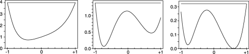
Figure 2: Error curve $|f-u|^{2}$ in the first three iteration steps for Example 7.1.

Table 3: The results of the algorithm proposed by Atkinson and Fedorov (1975b) in Example 7.1 (left part) and Example 7.2 (right part)

$\bolds{j}$	$\bolds{\|\psi\|}$	$\bolds{T(\xi_{j})}$	$\bolds{\frac{T(\xi_{j})}{\|\psi\|}}$	$\bolds{\|\psi\|}$	$\bolds{T(\xi_{j})}$	$\bolds{\frac{T(\xi_{j})}{\|\psi\|}}$
1	0.2172	0.1041	0.4791	0.0104	0.0033	0.3150
2	0.3995	0.0743	0.1860	0.0133	0.0034	0.2560
3	0.3189	0.0778	0.2440	0.0241	0.0045	0.1880
4	0.1539	0.1216	0.7903	0.0099	0.0055	0.5583
5	0.1974	0.1195	0.6055	0.0131	0.0055	0.4199
6	0.2337	0.1137	0.4868	0.0094	0.0063	0.6682
7	0.2045	0.1143	0.5592	0.0093	0.0060	0.6471
8	0.1347	0.1240	0.9206	0.0121	0.0062	0.5161
9	0.1732	0.1217	0.7029	0.0079	0.0065	0.8228
10	0.2055	0.1186	0.5773	0.0104	0.0064	0.6153
11	0.1791	0.1199	0.6694	0.0099	0.0064	0.6502
12	0.1356	0.1243	0.9165	0.0091	0.0065	0.7166
13	0.1651	0.1200	0.7267	0.0081	0.0066	0.8223
14	0.1640	0.1229	0.7493	0.0088	0.0065	0.7371
15	0.1714	0.1213	0.7078	0.0097	0.0065	0.6686
16	0.1362	0.1243	0.9130	0.0070	0.0067	0.9550

For the sake of comparison we also present in the left part of Table 3 the corresponding results for the first $16$ iterations of the algorithm proposed by Atkinson and Fedorov (1975b). This method starts with an initial guess, say $\xi_{0}$, and computes successively new designs $\xi_{1},\xi_{2},\ldots$ as follows:

[(1)]

At stage $s$ a point $x_{s+1}\in\mathcal{X}$ is determined such that $\psi(x_{s+1},\xi_{s})=\sup_{x\in\mathcal{X}}\psi(x,\xi_{s}),$ where the function $\psi$ is defined in (12).

The updated design $\xi_{s+1}$ is defined by $\xi_{s+1}=(1-\alpha_{s})\xi_{s}+\alpha_{s}\delta_{x_{s+1}},$ where $\delta_{x}$ is the Dirac measure at point $x$, and $(\alpha_{s})_{s\in\mathbb{N}_{0}}$ is any sequence of positive numbers satisfying $\alpha_{s}\rightarrow 0;$ $\sum^{\infty}_{s=0}\alpha_{s}=\infty;$ $\sum^{\infty}_{s=0}\alpha^{2}_{s}<\infty.$ This procedure provides the design

$$\xi=\pmatrix{-1&-0.2&-0.1&0&0.1&1\vspace*{2pt}\cr 0.23&0.18&0.12&0.1&0.17&0.20}$$

in $12$ iteration steps, and its efficiency is at least $92\%$. The final design contains an unnecessarily large support, although several design points with low weight have been removed during the computations. Note that neither the sup-norm of the function $\psi$ is decreasing, nor the lower bound $T(\xi)/\|\psi\|$ is increasing. In particular if the iteration is continued, the lower bound for the efficiency of the calculated design is decreasing again. This effect is at first compensated after the $16$th iteration, where the bound for the efficiency is $91\%$ (but not $92\%$ as after the $12$th iteration). This “oscillating behavior” was also observed in other examples and seems to be typical for the frequently used algorithm proposed by Atkinson and Fedorov (1975b).

Table 4: The results of the new algorithm for Example 7.2

	Part 1	Part 2
$\bolds{j}$	$\bolds{\|\varepsilon_{j,1}\|^{2}}$	$\bolds{\|\varepsilon_{j,2}\|^{2}}$	$\bolds{T(\xi_{j})}$	$\bolds{\frac{T(\xi_{j})}{\|\varepsilon_{j,2}\|^{2}}}$	Support	Reference set
$0$	1.253010					$\mathcal{S}\leftarrow\{1,2,4,6,8,10\}$
$1$	0.040044
$2$	0.012839	0.008738	0.005404	0.6184	$\{0.7,4.5,10\}$	$\mathcal{S}\leftarrow\mathcal{S}\cup\{0.7,4.5\}$
$3$	0.006957	0.006827	0.006757	0.9897	$\{0.5,3.6,10\}$	$\mathcal{S}\leftarrow\mathcal{S}\cup\{0.5,3.6\}$
$4$	0.006805	0.006797	0.006786	0.9996	$\{0.5,3.4,10\}$	$\mathcal{S}\leftarrow\mathcal{S}\cup\{3.4\}$
$5$	0.006793	0.006789	0.006786	0.9999
$6$	0.006788	0.006787	0.006786	0.9999

Example 7.2.

In order to demonstrate that the algorithm can be used when dealing with nonlinear regression models, we consider two rival models $\eta_{1}(x,\theta)=\frac{\theta_{11}x}{x+\theta_{12}}$, $\eta_{2}(x,\theta)=\theta_{21}(1-e^{-\theta_{22}x})$, where $\rho_{(1)}=(2.0,1.0)$ and $\rho_{(2)}=(2.5,0.5)$. The weights in the criterion (5) are $p_{1,2}=p_{2,1}=1/2$. The corresponding results are depicted in Table 4 and the Newton method is started with $\theta_{(1,2)}=(1,1)$, $\theta_{(2,1)}=(2,0.5)$ and $\mathcal{S}=\{1,2,4,6,8,10\}$. The degree of approximation is close to the optimum already after 6 iteration steps, and the guaranteed efficiency is $99.9\%$. The resulting design has masses $0.311$, $0.415$ and $0.274$ at the points $0.5$, $3.4$ and $10.0$, respectively, while the parameters of the solution of the approximation problem on the right-hand side of (13) are given (subject to rounding) by the parameters $\bar{\theta}_{(1,2)}=(3.008,1.809)$, and $\bar{\theta}_{(2,1)}=(1.721,0.865)$.

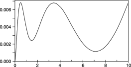
Figure 3: The function $\psi$ in the equivalence theorem (Theorem 3.1) for Example 7.2.

The determination of the parameter $\theta^{*}$ that minimizes $T(\xi)$ as defined in (4) is done by Newton’s method. It yields the best $\theta$ in a neighborhood of the computed solution. Therefore, we have also performed an extensive global search for the minimum and found a minimum that equals the result of Newton’s method up to rounding errors. Now, the plot of the corresponding function $\psi$ in the equivalence theorem (Theorem 3.1) is shown in Figure 3. We see that the design is in fact $T_{p}$-optimal discriminating. Note that the support of the resulting design consists of $3$ points in accordance with Conjecture 4.5. The corresponding results for the algorithm proposed by Atkinson and Fedorov (1975b) are displayed in the right part of Table 3. The algorithm needs $16$ iterations in order to find a design with masses $0.32$, $0.03$, $0.21$, $0.12$, $0.06$, $0.27$ at the (unnecessarily large set of) points $0.5$, $3.0$, $3.3$, $3.4$, $3.8$, $10$. Here the lower bound of the efficiency is only $95.5\%$ if we take the best information from the previous steps. The new algorithm is obviously much faster.

Example 7.3.

We consider $T_{p}$-optimal discriminating designs for the four competing dose–response models listed in Table 1 in the Introduction and the design space $\mathcal{X}=[0,500]$. Here, $d=6$ comparisons and $n=15$ parameters are involved. Moreover, the model $\eta_{4}$ is nonlinear. We use the weights $p_{i,j}=1/6$ if $i>j$ and $p_{i,j}=0$ otherwise in the criterion (5).

The corresponding results are displayed in Table 5, which shows that only $9$ iteration steps are required in order to obtain a design with at least $99.9\%$ efficiency. The resulting $T_{p}$-optimal discriminating design puts masses $0.255$, $0.212$, $0.358$, $0.175$ at the points $0$, $78$, $245$ and $500$, respectively.

We finally note that we were not able to find a design with a guaranteed efficiency of $80\%$ using the algorithm proposed by Atkinson and Fedorov (1975b).

Table 5: The results of the new algorithm for Example 7.3

	Part 1	Part 2
$\bolds{j}$	$\bolds{\|\varepsilon_{j,1}\|^{2}}$	$\bolds{\|\varepsilon_{j,2}\|^{2}}$	$\bolds{T(\xi_{j})}$	$\bolds{\frac{T(\xi_{j})}{\|\varepsilon_{j,2}\|^{2}}}$	Support	Reference set
$0$	16,661					$\mathcal{S}\leftarrow\{0,30,60,90,\ldots,450,500\}$
$1$	12,646
$2$	0.9727	8923	0275	0.0309	$\{0,50,290,450\}$	$\mathcal{S}\leftarrow\mathcal{S}\cup\{50,290\}$
$3$	0.8246	6901	0764	0.1108	$\{0,60,290,450\}$
$4$	0.5835	5081	2462	0.4846	$\{0,70,260,500\}$	$\mathcal{S}\leftarrow\mathcal{S}\cup\{70,260\}$
$5$	0.4543	4170	3016	0.7233	$\{0,80,250,500\}$	$\mathcal{S}\leftarrow\mathcal{S}\cup\{80,250\}$
$6$	0.4048	3619	3168	0.8754	$\{0,80,240,500\}$	$\mathcal{S}\leftarrow\{0,70,80,240,$
						$250,500\}$
$7$	0.3446	3270	3194	0.9989
$8$	0.3201	3199	3195	0.9980	$\{0,78,240,500\}$	$\mathcal{S}\leftarrow\mathcal{S}\cup\{78\}$
$9$	0.3197	3196	3195	0.9998

8 Concluding remarks

Our main theoretical result relates $T_{p}$-optimal discriminating designs to an approximation problem for vector-valued functions (Theorem 3.2). By duality theory we show that there exist $T_{p}$-optimal designs with at most $n+1$ support points, where $n$ is the number of parameters in the approximation problem (which coincides with the total number of parameters of all regression functions used in the comparisons). These results are sufficient if we are interested only one or two comparisons among the rival models. In this case the computations can be done by an exchange-type algorithm that was already proposed by Atkinson and Fedorov (1975b). This procedure is still the common tool for dealing with design problems whenever $d=1$ or $d=2$.

The situation is different and the construction of $T_{p}$-optimal discriminating designs becomes extremely difficult and challenging if three or more comparisons are involved. The number of support points can now be much smaller than $n+1$, where $n$ is the total number of parameters of the models involved in the $T_{p}$-optimality criterion. Although a reduction of this number was already observed in the case $d=2$, the amount of the reduction and its impact become clear only when optimal discriminating design problems with $d\geq 3$ pairwise comparisons are studied. For example, we have $n=15$ parameters in the dose-finding problems listed in Table 1, but the support of the $T_{p}$-optimal discriminating design consists of only 4 points.

Therefore, there are substantial differences between our new algorithm and the generalization of the method by Atkinson and Fedorov (1975b) beyond the case $d=1$. Our algorithm is based on the related approximation problem (Theorem 3.2), and additionally we also add combinatorial aspects [addition (iii) in Section 6.1], which accelerate the speed of convergence. Dual linear programs associated to small subproblems determine the support of the resulting design and prevent the algorithm from providing designs with too many support points. The masses are simultaneously computed by a stabilized version of the equations in Corollary 3.4, while the commonly used algorithms in each iteration step involve an update of the mass at only one point and a renormalization.

Our numerical examples in Section 7 and in the supplementary material [Braess and Dette (2013)] show that the new algorithm is able to solve $T_{p}$-optimal discriminating design problems of higher dimensions in situations where the classical methods fail.

References

- Atkinson (2008a) {barticle}[mr] \bauthor\bsnmAtkinson, \bfnmAnthony C.\binitsA. C. (\byear2008a). \btitleExamples of the use of an equivalence theorem in constructing optimum experimental designs for random-effects nonlinear regression models. \bjournalJ. Statist. Plann. Inference \bvolume138 \bpages2595–2606. \biddoi=10.1016/j.jspi.2008.03.002, issn=0378-3758, mr=2439971 \bptokimsref \endbibitem
- Atkinson (2008b) {barticle}[mr] \bauthor\bsnmAtkinson, \bfnmA. C.\binitsA. C. (\byear2008b). \btitleDT-optimum designs for model discrimination and parameter estimation. \bjournalJ. Statist. Plann. Inference \bvolume138 \bpages56–64. \biddoi=10.1016/j.jspi.2007.05.024, issn=0378-3758, mr=2369613 \bptokimsref \endbibitem
- Atkinson and Fedorov (1975a) {barticle}[mr] \bauthor\bsnmAtkinson, \bfnmA. C.\binitsA. C. and \bauthor\bsnmFedorov, \bfnmV. V.\binitsV. V. (\byear1975a). \btitleOptimal design: Experiments for discriminating between several models. \bjournalBiometrika \bvolume62 \bpages289–303. \bidissn=0006-3444, mr=0381163 \bptokimsref \endbibitem
- Atkinson and Fedorov (1975b) {barticle}[mr] \bauthor\bsnmAtkinson, \bfnmA. C.\binitsA. C. and \bauthor\bsnmFedorov, \bfnmV. V.\binitsV. V. (\byear1975b). \btitleThe design of experiments for discriminating between two rival models. \bjournalBiometrika \bvolume62 \bpages57–70. \bidissn=0006-3444, mr=0370955 \bptokimsref \endbibitem
- Braess and Dette (2013) {bmisc}[auto] \bauthor\bsnmBraess, \bfnmDietrich\binitsD. and \bauthor\bsnmDette, \bfnmHolger\binitsH. (\byear2013). \bhowpublishedSupplement to “Optimal discriminating designs for several competing regression models.” DOI:\doiurl10.1214/13-AOS1103SUPP. \bptokimsref \endbibitem
- Bretz, Pinheiro and Branson (2005) {barticle}[mr] \bauthor\bsnmBretz, \bfnmF.\binitsF., \bauthor\bsnmPinheiro, \bfnmJ. C.\binitsJ. C. and \bauthor\bsnmBranson, \bfnmM.\binitsM. (\byear2005). \btitleCombining multiple comparisons and modeling techniques in dose–response studies. \bjournalBiometrics \bvolume61 \bpages738–748. \biddoi=10.1111/j.1541-0420.2005.00344.x, issn=0006-341X, mr=2196162 \bptokimsref \endbibitem
- Brosowski (1968) {bbook}[mr] \bauthor\bsnmBrosowski, \bfnmBruno\binitsB. (\byear1968). \btitleNicht-Lineare Tschebyscheff-Approximation. \bpublisherBibliographisches Institut, \blocationMannheim. \bidmr=0228903 \bptokimsref \endbibitem
- Cheney (1966) {bbook}[author] \bauthor\bsnmCheney, \bfnmE. W\binitsE. W. (\byear1966). \btitleIntroduction to Approximation Theory. \bpublisherMcGraw-Hill, \blocationNew York. \bptokimsref \endbibitem
- Dette and Haller (1998) {barticle}[mr] \bauthor\bsnmDette, \bfnmHolger\binitsH. and \bauthor\bsnmHaller, \bfnmGerd\binitsG. (\byear1998). \btitleOptimal designs for the identification of the order of a Fourier regression. \bjournalAnn. Statist. \bvolume26 \bpages1496–1521. \biddoi=10.1214/aos/1024691251, issn=0090-5364, mr=1647689 \bptokimsref \endbibitem
- Dette, Melas and Shpilev (2012) {barticle}[mr] \bauthor\bsnmDette, \bfnmHolger\binitsH., \bauthor\bsnmMelas, \bfnmViatcheslav B.\binitsV. B. and \bauthor\bsnmShpilev, \bfnmPetr\binitsP. (\byear2012). \btitle-optimal designs for discrimination between two polynomial models. \bjournalAnn. Statist. \bvolume40 \bpages188–205. \biddoi=10.1214/11-AOS956, issn=0090-5364, mr=3013184 \bptokimsref \endbibitem
- Dette and Titoff (2009) {barticle}[mr] \bauthor\bsnmDette, \bfnmHolger\binitsH. and \bauthor\bsnmTitoff, \bfnmStefanie\binitsS. (\byear2009). \btitleOptimal discrimination designs. \bjournalAnn. Statist. \bvolume37 \bpages2056–2082. \biddoi=10.1214/08-AOS635, issn=0090-5364, mr=2533479 \bptokimsref \endbibitem
- Fedorov (1980) {bincollection}[mr] \bauthor\bsnmFedorov, \bfnmV.\binitsV. (\byear1980). \btitleDesign of model testing experiments. In \bbooktitleSymposia Mathematica, Vol. XXV (Conf., INDAM, Rome, 1979) \bpages171–180. \bpublisherAcademic Press, \blocationLondon. \bidmr=0618870 \bptnotecheck year\bptokimsref \endbibitem
- Fedorov and Khabarov (1986) {barticle}[mr] \bauthor\bsnmFedorov, \bfnmV.\binitsV. and \bauthor\bsnmKhabarov, \bfnmV.\binitsV. (\byear1986). \btitleDuality of optimal designs for model discrimination and parameter estimation. \bjournalBiometrika \bvolume73 \bpages183–190. \biddoi=10.1093/biomet/73.1.183, issn=0006-3444, mr=0836446 \bptokimsref \endbibitem
- Kiefer (1974) {barticle}[mr] \bauthor\bsnmKiefer, \bfnmJ.\binitsJ. (\byear1974). \btitleGeneral equivalence theory for optimum designs (approximate theory). \bjournalAnn. Statist. \bvolume2 \bpages849–879. \bidissn=0090-5364, mr=0356386 \bptokimsref \endbibitem
- López-Fidalgo, Tommasi and Trandafir (2007) {barticle}[mr] \bauthor\bsnmLópez-Fidalgo, \bfnmJ.\binitsJ., \bauthor\bsnmTommasi, \bfnmC.\binitsC. and \bauthor\bsnmTrandafir, \bfnmP. C.\binitsP. C. (\byear2007). \btitleAn optimal experimental design criterion for discriminating between non-normal models. \bjournalJ. R. Stat. Soc. Ser. B Stat. Methodol. \bvolume69 \bpages231–242. \biddoi=10.1111/j.1467-9868.2007.00586.x, issn=1369-7412, mr=2325274 \bptokimsref \endbibitem
- Meinardus (1967) {bbook}[author] \bauthor\bsnmMeinardus, \bfnmG.\binitsG. (\byear1967). \btitleApproximation of Functions: Theory and Numerical Methods. \bpublisherSpringer, \blocationBerlin. \bptokimsref \endbibitem
- Papadimitriou and Steiglitz (1998) {bbook}[mr] \bauthor\bsnmPapadimitriou, \bfnmChristos H.\binitsC. H. and \bauthor\bsnmSteiglitz, \bfnmKenneth\binitsK. (\byear1998). \btitleCombinatorial Optimization: Algorithms and Complexity, \bedition2nd ed. \bpublisherDover, \blocationMineola, NY. \bidmr=1637890 \bptokimsref \endbibitem
- Pinheiro, Bretz and Branson (2006) {bincollection}[author] \bauthor\bsnmPinheiro, \bfnmJ.\binitsJ., \bauthor\bsnmBretz, \bfnmF.\binitsF. and \bauthor\bsnmBranson, \bfnmM.\binitsM. (\byear2006). \btitleAnalysis of dose–response studies: Modeling approaches. In \bbooktitleDose Finding in Drug Development (\beditor\bfnmN.\binitsN. \bsnmTing, ed.) \bpages146–171. \bpublisherSpringer, \blocationNew York. \bptokimsref \endbibitem
- Seber and Wild (1989) {bbook}[mr] \bauthor\bsnmSeber, \bfnmG. A. F.\binitsG. A. F. and \bauthor\bsnmWild, \bfnmC. J.\binitsC. J. (\byear1989). \btitleNonlinear Regression. \bpublisherWiley, \blocationNew York. \biddoi=10.1002/0471725315, mr=0986070 \bptokimsref \endbibitem
- Song and Wong (1999) {barticle}[mr] \bauthor\bsnmSong, \bfnmDale\binitsD. and \bauthor\bsnmWong, \bfnmWeng Kee\binitsW. K. (\byear1999). \btitleOn the construction of -optimal designs. \bjournalStatist. Sinica \bvolume9 \bpages263–272. \bidissn=1017-0405, mr=1678893 \bptokimsref \endbibitem
- Stigler (1971) {barticle}[author] \bauthor\bsnmStigler, \bfnmS.\binitsS. (\byear1971). \btitleOptimal experimental design for polynomial regression. \bjournalJ. Amer. Statist. Assoc. \bvolume66 \bpages311–318. \bptokimsref \endbibitem
- Tommasi (2009) {barticle}[mr] \bauthor\bsnmTommasi, \bfnmC.\binitsC. (\byear2009). \btitleOptimal designs for both model discrimination and parameter estimation. \bjournalJ. Statist. Plann. Inference \bvolume139 \bpages4123–4132. \biddoi=10.1016/j.jspi.2009.05.042, issn=0378-3758, mr=2558355 \bptokimsref \endbibitem
- Tommasi and López-Fidalgo (2010) {barticle}[mr] \bauthor\bsnmTommasi, \bfnmC.\binitsC. and \bauthor\bsnmLópez-Fidalgo, \bfnmJ.\binitsJ. (\byear2010). \btitleBayesian optimum designs for discriminating between models with any distribution. \bjournalComput. Statist. Data Anal. \bvolume54 \bpages143–150. \biddoi=10.1016/j.csda.2009.07.022, issn=0167-9473, mr=2558465 \bptokimsref \endbibitem
- Uciński and Bogacka (2005) {barticle}[mr] \bauthor\bsnmUciński, \bfnmDariusz\binitsD. and \bauthor\bsnmBogacka, \bfnmBarbara\binitsB. (\byear2005). \btitle-optimum designs for discrimination between two multiresponse dynamic models. \bjournalJ. R. Stat. Soc. Ser. B Stat. Methodol. \bvolume67 \bpages3–18. \biddoi=10.1111/j.1467-9868.2005.00485.x, issn=1369-7412, mr=2136636 \bptokimsref \endbibitem
- Wiens (2009) {barticle}[mr] \bauthor\bsnmWiens, \bfnmDouglas P.\binitsD. P. (\byear2009). \btitleRobust discrimination designs. \bjournalJ. R. Stat. Soc. Ser. B Stat. Methodol. \bvolume71 \bpages805–829. \biddoi=10.1111/j.1467-9868.2009.00711.x, issn=1369-7412, mr=2750096 \bptokimsref \endbibitem