Multiclass Semi-Supervised Learning on Graphs
using Ginzburg-Landau Functional Minimization

Abstract

We present a graph-based variational algorithm for classification of high-dimensional data, generalizing the binary diffuse interface model to the case of multiple classes. Motivated by total variation techniques, the method involves minimizing an energy functional made up of three terms. The first two terms promote a stepwise continuous classification function with sharp transitions between classes, while preserving symmetry among the class labels. The third term is a data fidelity term, allowing us to incorporate prior information into the model in a semi-supervised framework. The performance of the algorithm on synthetic data, as well as on the COIL and MNIST benchmark datasets, is competitive with state-of-the-art graph-based multiclass segmentation methods.

1 Introduction

Many tasks in pattern recognition and machine learning rely on the ability to quantify local similarities in data, and to infer meaningful global structure from such local characteristics [8]. In the classification framework, the desired global structure is a descriptive partition of the data into categories or classes. Many studies have been devoted to the binary classification problems. The multiple-class case, where data are partitioned into more than two clusters, is more challenging. One approach is to treat the problem as a series of binary classification problems [1]. In this paper, we develop an alternative method, involving a multiple-class extension of the diffuse interface model introduced in [4].

The diffuse interface model by Bertozzi and Flenner combines methods for diffusion on graphs with efficient partial differential equation techniques to solve binary segmentation problems. As with other methods inspired by physical phenomena [3, 17, 21], it requires the minimization of an energy expression, specifically the Ginzburg-Landau (GL) energy functional. The formulation generalizes the GL functional to the case of functions defined on graphs, and its minimization is related to the minimization of weighted graph cuts [4]. In this sense, it parallels other techniques based on inference on graphs via diffusion operators or function estimation [8, 7, 31, 26, 28, 5, 25, 15].

Multiclass segmentation methods that cast the problem as a series of binary classification problems use a number of different strategies: (i) deal directly with some binary coding or indicator for the labels [9, 28], (ii) build a hierarchy or combination of classifiers based on the one-vs-all approach or on class rankings [14, 13] or (iii) apply a recursive partitioning scheme consisting of successively subdividing clusters, until the desired number of classes is reached [25, 15]. While there are advantages to these approaches, such as possible robustness to mislabeled data, there can be a considerable number of classifiers to compute, and performance is affected by the number of classes to partition.

In contrast, we propose an extension of the diffuse interface model that obtains a simultaneous segmentation into multiple classes. The multiclass extension is built by modifying the GL energy functional to remove the prejudicial effect that the order of the labelings, given by integer values, has in the smoothing term of the original binary diffuse interface model. A new term that promotes homogenization in a multiclass setup is introduced. The expression penalizes data points that are located close in the graph but are not assigned to the same class. This penalty is applied independently of how different the integer values are, representing the class labels. In this way, the characteristics of the multiclass classification task are incorporated directly into the energy functional, with a measure of smoothness independent of label order, allowing us to obtain high-quality results. Alternative multiclass methods minimize a Kullback-Leibler divergence function [23] or expressions involving the discrete Laplace operator on graphs [30, 28].

This paper is organized as follows. Section 2 reviews the diffuse interface model for binary classification, and describes its application to semi-supervised learning. Section 3 discusses our proposed multiclass extension and the corresponding computational algorithm. Section 4 presents results obtained with our method. Finally, section 5 draws conclusions and delineates future work.

2 Data Segmentation with the Ginzburg-Landau Model

The diffuse interface model [4] is based on a continuous approach, using the Ginzburg-Landau (GL) energy functional to measure the quality of data segmentation. A good segmentation is characterized by a state with small energy. Let $u(\boldsymbol{x})$ be a scalar field defined over a space of arbitrary dimensionality, and representing the state of the system. The GL energy is written as the functional

$$\mathrm{GL}(u)=\frac{\epsilon}{2}\int\!|\nabla u|^{2}\;d\boldsymbol{x}+\frac{1}{\epsilon}\int\!\Phi(u)\;d\boldsymbol{x},$$ (1)

with $\nabla$ denoting the spatial gradient operator, $\epsilon>0$ a real constant value, and $\Phi$ a double well potential with minima at $\pm 1$:

$$\Phi(u)=\frac{1}{4}\left(u^{2}-1\right)^{2}.$$ (2)

Segmentation requires minimizing the GL functional. The norm of the gradient is a smoothing term that penalizes variations in the field $u$. The potential term, on the other hand, compels $u$ to adopt the discrete labels of $+1$ or $-1$, clustering the state of the system around two classes. Jointly minimizing these two terms pushes the system domain towards homogeneous regions with values close to the minima of the double well potential, making the model appropriate for binary segmentation.

The smoothing term and potential term are in conflict at the interface between the two regions, with the first term favoring a gradual transition, and the second term penalizing deviations from the discrete labels. A compromise between these conflicting goals is established via the constant $\epsilon$. A small value of $\epsilon$ denotes a small length transition and a sharper interface, while a large $\epsilon$ weights the gradient norm more, leading to a slower transition. The result is a diffuse interface between regions, with sharpness regulated by $\epsilon$.

It can be shown that in the limit $\epsilon\to 0$ this function approximates the total variation (TV) formulation in the sense of functional ($\Gamma$) convergence [18], producing piecewise constant solutions but with greater computational efficiency than conventional TV minimization methods. Thus, the diffuse interface model provides a framework to compute piecewise constant functions with diffuse transitions, approaching the ideal of the TV formulation, but with the advantage that the smooth energy functional is more tractable numerically and can be minimized by simple numerical methods such as gradient descent.

The GL energy has been used to approximate the TV norm for image segmentation [4] and image inpainting [3, 10]. Furthermore, a calculus on graphs equivalent to TV has been introduced in [12, 25].

Application of Diffuse Interface Models to Graphs

An undirected, weighted neighborhood graph is used to represent the local relationships in the data set. This is a common technique to segment classes that are not linearly separable. In the $N$-neighborhood graph model, each vertex $v_{i}\in V$ of the graph corresponds to a data point with feature vector $\boldsymbol{x}_{i}$, while the weight $w_{ij}$ is a measure of similarity between $v_{i}$ and $v_{j}$. Moreover, it satisfies the symmetry property $w_{ij}=w_{ji}$. The neighborhood is defined as the set of $N$ closest points in the feature space. Accordingly, edges exist between each vertex and the vertices of its $N$-nearest neighbors. Following the approach of [4], we calculate weights using the local scaling of Zelnik-Manor and Perona [29],

$$w_{ij}=\exp\left(-\frac{||\boldsymbol{x}_{i}-\boldsymbol{x}_{j}||^{2}}{\tau(\boldsymbol{x}_{i})\;\tau(\boldsymbol{x}_{j})}\right).$$ (3)

Here, $\tau(\boldsymbol{x}_{i})=||\boldsymbol{x}_{i}-\boldsymbol{x}^{M}_{i}||$ defines a local value for each $\boldsymbol{x}_{i}$, where $\boldsymbol{x}^{M}_{i}$ is the position of the $M$th closest data point to $\boldsymbol{x}_{i}$, and $M$ is a global parameter.

It is convenient to express calculations on graphs via the graph Laplacian matrix, denoted by $\mathbf{L}$. The procedure we use to build the graph Laplacian is as follows.

1. Compute the similarity matrix $\mathbf{W}$ with components $w_{ij}$ defined in (3). As the neighborhood relationship is not symmetric, the resulting matrix $\mathbf{W}$ is also not symmetric. Make it a symmetric matrix by connecting vertices $v_{i}$ and $v_{j}$ if $v_{i}$ is among the $N$-nearest neighbors of $v_{j}$ or if $v_{j}$ is among the $N$-nearest neighbors of $v_{i}$ [27].

2. Define $\mathbf{D}$ as a diagonal matrix whose $i$th diagonal element represents the degree of the vertex $v_{i}$, evaluated as

   $$d_{i}=\sum_{j}w_{ij}.$$ (4)

3. Calculate the graph Laplacian: $\mathbf{L}=\mathbf{D}-\mathbf{W}$.

Generally, the graph Laplacian is normalized to guarantee spectral convergence in the limit of large sample size [27]. The symmetric normalized graph Laplacian ${\mathbf{L}\boldsymbol{{}_{s}}}$ is defined as

$${\mathbf{L}\boldsymbol{{}_{s}}}=\mathbf{D}^{-1/2}\;\mathbf{L}\;\mathbf{D}^{-1/2}=\mathbf{I}-\mathbf{D}^{-1/2}\;\mathbf{W}\;\mathbf{D}^{-1/2}.$$ (5)

Data segmentation can now be carried out through a graph-based formulation of the GL energy. To implement this task, a fidelity term is added to the functional as initially suggested in [11]. This enables the specification of a priori information in the system, for example the known labels of certain points in the data set. This kind of setup is called semi-supervised learning (SSL). The discrete GL energy for SSL on graphs can be written as [4]:

$$\mathrm{GL}_{\mathrm{SSL}}(\boldsymbol{u}) = \frac{\epsilon}{2}\langle\boldsymbol{u},{\mathbf{L}\boldsymbol{{}_{s}}}\boldsymbol{u}\rangle+\frac{1}{\epsilon}\sum_{v_{i}\in V}\Phi(u(v_{i}))+\sum_{v_{i}\in V}\frac{\mu(v_{i})}{2}\;\left(u(v_{i})-\hat{u}(v_{i})\right)^{2}$$ (7)

$$= \frac{\epsilon}{4}\sum_{v_{i},v_{j}\in V}w_{ij}\left(\frac{u(v_{i})}{\sqrt{d_{i}}}-\frac{u(v_{j})}{\sqrt{d_{j}}}\right)^{2}+\frac{1}{\epsilon}\sum_{v_{i}\in V}\Phi(u(v_{i}))+$$

$$\sum_{v_{i}\in V}\frac{\mu(v_{i})}{2}\;\left(u(v_{i})-\hat{u}(v_{i})\right)^{2}.$$

In the discrete formulation, $\boldsymbol{u}$ is a vector whose component $u(v_{i})$ represents the state of the vertex $v_{i}$, $\epsilon>0$ is a real constant characterizing the smoothness of the transition between classes, and $\mu(v_{i})$ is a fidelity weight taking value $\mu>0$ if the label $\hat{u}(v_{i})$ (i.e. class) of the data point associated with vertex $v_{i}$ is known beforehand, or $\mu(v_{i})=0$ if it is not known (semi-supervised).

Minimizing the functional simulates a diffusion process on the graph. The information of the few labels known is propagated through the discrete structure by means of the smoothing term, while the potential term clusters the vertices around the states $\pm 1$ and the fidelity term enforces the known labels. The energy minimization process itself attempts to reduce the interface regions. Note that in the absence of the fidelity term, the process could lead to a trivial steady-state solution of the diffusion equation, with all data points assigned the same label.

The final state $u(v_{i})$ of each vertex is obtained by thresholding, and the resulting homogeneous regions with labels of $+1$ and $-1$ constitute the two-class data segmentation.

3 Multiclass Extension

The double-well potential in the diffuse interface model for SSL drives the state of the system towards two definite labels. Multiple-class segmentation requires a more general potential function $\Phi_{M}(u)$ that allows clusters around more than two labels. For this purpose, we use the periodic-well potential suggested by Li and Kim [21],

$$\Phi_{M}(u)=\frac{1}{2}\,\{u\}^{2}\,(\{u\}-1)^{2},$$ (8)

where $\{u\}$ denotes the fractional part of $u$,

$$\{u\}=u-\lfloor u\rfloor,$$ (9)

and $\lfloor u\rfloor$ is the largest integer not greater than $u$.

This periodic potential well promotes a multiclass solution, but the graph Laplacian term in Equation (7) also requires modification for effective calculations due to the fixed ordering of class labels in the multiple class setting. The graph Laplacian term penalizes large changes in the spatial distribution of the system state more than smaller gradual changes. In a multiclass framework, this implies that the penalty for two spatially contiguous classes with different labels may vary according to the (arbitrary) ordering of the labels.

This phenomenon is shown in Fig. 1. Suppose that the goal is to segment the image into three classes: class 0 composed by the black region, class 1 composed by the gray region and class 2 composed by the white region. It is clear that the horizontal interfaces comprise a jump of size 1 (analogous to a two class segmentation) while the vertical interface implies a jump of size 2. Accordingly, the smoothing term will assign a higher cost to the vertical interface, even though from the point of view of the classification, there is no specific reason for this. In this example, the problem cannot be solved with a different label assignment. There will always be an interface with higher costs than others independent of the integer values used.

Thus, the multiclass approach breaks the symmetry among classes, influencing the diffuse interface evolution in an undesirable manner. Eliminating this inconvenience requires restoring the symmetry, so that the difference between two classes is always the same, regardless of their labels. This objective is achieved by introducing a new class difference measure.

Figure 1: Three-class segmentation. Black: class 0. Gray: class 1. White: class 2.

3.1 Generalized Difference Function

The final class labels are determined by thresholding each vertex $u(v_{i})$, with the label $y_{i}$ set to the nearest integer:

$$y_{i}=\left\lfloor u(v_{i})+\frac{1}{2}\right\rfloor.$$ (10)

The boundaries between classes then occur at half-integer values corresponding to the unstable equilibrium states of the potential well. Define the function $\hat{r}(x)$ to represent the distance to the nearest half-integer:

$$\hat{r}(x)=\left|\frac{1}{2}-\{x\}\right|.$$ (11)

A schematic of $\hat{r}(x)$ is depicted in Fig. 2. The $\hat{r}(x)$ function is used to define a generalized difference function between classes that restores symmetry in the energy functional. Define the generalized difference function $\rho$ as:

$$\rho(u(v_{i}),u(v_{j}))=\left\{\begin{array}[]{lll}\hat{r}(u(v_{i}))+\hat{r}(u(v_{j}))&&y_{i}\neq y_{j}\\ &&\\ \left|\hat{r}(u(v_{i}))-\hat{r}(u(v_{j}))\right|&&y_{i}=y_{j}\end{array}\right.$$ (12)

Thus, if the vertices are in different classes, the difference $\hat{r}(x)$ between each state’s value and the nearest half-integer is added, whereas if they are in the same class, these differences are subtracted. The function $\rho(x,y)$ corresponds to the tree distance (see Fig. 2). Strictly speaking, $\rho$ is not a metric since it does not satisfy $\rho(x,y)=0\Rightarrow x=y$. Nevertheless, the cost of interfaces between classes becomes the same regardless of class labeling when this generalized distance function is implemented.

Figure 2: Schematic interpretation of generalized difference: $\hat{r}(x)$ measures distance to nearest half-integer, and $\rho$ is a tree distance measure.

The GL energy functional for SSL, using the new generalized difference function $\rho$ and the periodic potential, is expressed as

$$\mathrm{MGL}_{\mathrm{SSL}}(\boldsymbol{u}) = \frac{\epsilon}{2}\sum_{v_{i}\in V}\sum_{v_{j}\in V}\frac{w_{ij}}{\sqrt{d_{i}d_{j}}}\,\left[\rho(u(v_{i}),u(v_{j}))\,\right]^{2}+$$ (13)

$$\frac{1}{2\epsilon}\sum_{v_{i}\in V}\{u(v_{i})\}^{2}\,(\{u(v_{i})\}-1)^{2}+$$

$$\sum_{v_{i}\in V}\frac{\mu(v_{i})}{2}\;\left(u(v_{i})-\hat{u}(v_{i})\right)^{2}.$$

Note that the smoothing term in this functional is composed of an operator that is not just a generalization of the normalized symmetric Laplacian ${\mathbf{L}\boldsymbol{{}_{s}}}$. The new smoothing operation, written in terms of the generalized distance function $\rho$, constitutes a non-linear operator that is a symmetrization of a different normalized Laplacian, the random walk Laplacian $\mathbf{L}\boldsymbol{{}_{w}}=\mathbf{D}^{-1}\mathbf{L}=\mathbf{I}-\mathbf{D}^{-1}\mathbf{W}$ [27]. The reason is as follows. The Laplacian $\mathbf{L}$ satisfies

$$(\mathbf{L}\boldsymbol{u})_{i}=\sum_{j}w_{ij}\left(u_{i}-u_{j}\right)$$

and $\mathbf{L}\boldsymbol{{}_{w}}$ satisfies

$$(\mathbf{L}\boldsymbol{{}_{w}}\boldsymbol{u})_{i}=\sum_{j}\frac{w_{ij}}{d_{i}}\left(u_{i}-u_{j}\right).$$

Now replace $w_{ij}/{d_{i}}$ in the latter expression with the symmetric form ${w_{ij}}/{\sqrt{d_{i}d_{j}}}$. This is equivalent to constructing a reweighted graph with weights $\widehat{w}_{ij}$ given by:

$$\widehat{w}_{ij}=\frac{w_{ij}}{\sqrt{d_{i}d_{j}}}.$$

The corresponding reweighted Laplacian $\mathbf{\widehat{L}}$ satisfies:

$$(\mathbf{\widehat{L}}\boldsymbol{u})_{i}=\sum_{j}\widehat{w}_{ij}\left(u_{i}-u_{j}\right)=\sum_{j}\frac{w_{ij}}{\sqrt{d_{i}d_{j}}}\left(u_{i}-u_{j}\right),$$ (14)

and

$$\langle\boldsymbol{u},\mathbf{\widehat{L}}\boldsymbol{u}\rangle=\frac{1}{2}\sum_{i,j}\frac{w_{ij}}{\sqrt{d_{i}d_{j}}}\left(u_{i}-u_{j}\right)^{2}.$$ (15)

While $\mathbf{\widehat{L}}=\mathbf{\widehat{D}}-\mathbf{\widehat{W}}$ is not a standard normalized Laplacian, it does have the desirable properties of stability and consistency with increasing sample size of the data set, and of satisfying the conditions for $\Gamma$-convergence to TV in the $\epsilon\to 0$ limit [2]. It also generalizes to the tree distance more easily than does ${\mathbf{L}\boldsymbol{{}_{s}}}$. Replacing the difference $\left(u_{i}-u_{j}\right)^{2}$ with the generalized difference $\left[\rho(u_{i},u_{j})\right]^{2}$ then gives the new smoothing multiclass term of equation (13). Empirically, this new term seems to perform well even though the normalization procedure differs from the binary case.

By implementing the generalized difference function on a tree, the cost of interfaces between classes becomes the same regardless of class labeling.

3.2 Computational Algorithm

The GL energy functional given by (13) may be minimized iteratively, using gradient descent:

$$u_{i}^{n+1}=u_{i}^{n}-dt\,\left[\frac{\delta\mathrm{MGL}_{\mathrm{SSL}}}{\delta u_{i}}\right],$$ (16)

where $u_{i}$ is a shorthand for $u(v_{i})$, $dt$ represents the time step and the gradient direction is given by:

$$\frac{\delta\mathrm{MGL}_{\mathrm{SSL}}}{\delta u_{i}}=\epsilon\;\hat{R}(u_{i}^{n})+\frac{1}{\epsilon}\Phi_{M}^{\prime}(u_{i}^{n})+\mu_{i}\left(u_{i}^{n}-\hat{u}_{i}\right)$$ (17)

$$\hat{R}(u_{i}^{n})=\sum_{j}\frac{w_{ij}}{\sqrt{d_{i}d_{j}}}\left[\hat{r}(u_{i}^{n})\pm\hat{r}(u_{j}^{n})\right]\hat{r}^{\prime}(u_{i}^{n})$$ (18)

$$\Phi_{M}^{\prime}(u_{i}^{n})=2\;\{u_{i}^{n}\}^{3}-3\;\{u_{i}^{n}\}^{2}+\{u_{i}^{n}\}$$ (19)

The gradient of the generalized difference function $\rho$ is not defined at half integer values. Hence, we modify the method using a greedy strategy: after detecting that a vertex changes class, the new class that minimizes the smoothing term is selected, and the fractional part of the state computed by the gradient descent update is preserved. Consequently, the new state of vertex $i$ is the result of gradient descent, but if this causes a change in class, then a new state is determined.

Algorithm 1 Calculate $\boldsymbol{u}$

0:  $\epsilon,dt,N_{D},n_{\mathrm{max}},K$

0:  $\mathrm{out}=\boldsymbol{u^{\mathrm{end}}}$

  for $i=1\to N_{D}$ do

     $u_{i}^{~{}0}\leftarrow rand((0,K))-\frac{1}{2}.\quad\mathrm{If~{}}\mu_{i}>0,~{}u_{i}^{~{}0}\leftarrow\hat{u}_{i}$

  end for

  for $n=1\to n_{\mathrm{max}}$ do

     for $i=1\to N_{D}$ do

        $u_{i}^{n+1}\leftarrow u_{i}^{n}-dt\left(\epsilon\>\hat{R}(u_{i}^{n})+\frac{1}{\epsilon}\>\Phi_{M}^{\prime}(u_{i}^{n})+\mu_{i}\left(u_{i}^{n}-\hat{u}_{i}\right)\right)$

        if $\mathrm{Label}(u_{i}^{n+1})\neq\mathrm{Label}(u_{i}^{n})$ then

           $\hat{k}=\arg\min_{\;0\leq k<K}\;\sum_{j}\frac{w_{ij}}{\sqrt{d_{i}d_{j}}}\,\left[\rho(k+\{u_{i}^{n+1}\},u_{j}^{n+1})\,\right]^{2}$

           $u_{i}^{n+1}\leftarrow\hat{k}+\{u_{i}^{n+1}\}$

        end if

     end for

  end for

Specifically, let $k$ represent an integer in the range of the problem, i.e. $k\in[0,K-1]$, where $K$ is the number of classes in the problem. Given the fractional part $\{u\}$ resulting from the gradient descent update, find the integer $k$ that minimizes $\sum_{j}\frac{w_{ij}}{\sqrt{d_{i}d_{j}}}\,\left[\rho(k+\{u_{i}\},u_{j})\,\right]^{2}$, the smoothing term in the energy functional, and use $k+\{u_{i}\}$ as the new vertex state. A summary of the procedure is shown in Algorithm 1 with $N_{D}$ representing the number of points in the data set and $n_{\mathrm{max}}$ denoting the maximum number of iterations.

4 Results

The performance of the multiclass diffuse interface model is evaluated using a number of data sets from the literature, with differing characteristics. Data and image segmentation problems are considered on synthetic and real data sets.

4.1 Synthetic Data

4.1.1 Three Moons.

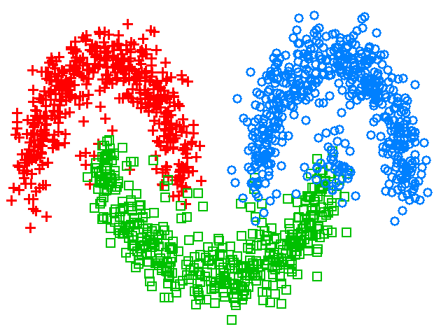
A synthetic three-class segmentation problem is constructed following an analogous procedure to the one used in [5] for “two moon” binary classification. Three half circles (“three moons”) are generated in $\mathbb{R}^{2}$. The two top circles have radius $1$ and are centered at $(0,0)$ and $(3,0)$. The bottom half circle has radius $1.5$ and is centered at $(1.5,0.4)$. 1,500 data points (500 from each of these half circles) are sampled and embedded in $\mathbb{R}^{100}$. The embedding is completed by adding Gaussian noise with $\sigma^{2}=0.02$ to each of the 100 components for each data point. The dimensionality of the data set, together with the noise, make this a nontrivial problem.

The symmetric normalized graph Laplacian is computed for a local scaling graph using $N=10$ nearest neighbors and local scaling based on the $M=10^{th}$ closest point. The fidelity term is constructed by labeling 25 points per class, 75 points in total, corresponding to only 5% of the points in the data set. The multiclass GL method was further refined by geometrically decreasing $\epsilon$ over the course of the minimization process, from $\epsilon_{0}$ to $\epsilon_{f}$ by factors of $1-\Delta_{\epsilon}$ ($n_{\mathrm{max}}$ iterations per value of $\epsilon$), to allow sharper transitions between states as in [4]. Table 1 specifies the parameters used. Average accuracies and computation times are reported over 100 runs. Results for $k$-means and spectral clustering (obtained by applying $k$-means to the first 3 eigenvectors of $\mathbf{L}\boldsymbol{{}_{s}}$) are included as reference.

Table 1: Three-moons results

Method	Parameters	Correct % (stddev %)	Time [s]
$k$-means	–	72.1 (0.35)	0.66
Spectral clustering	3 eigenvectors	80.0 (0.59)	0.02
Multiclass GL	${\mu=30}$, ${\epsilon=1}$, ${dt=0.01}$,	95.1 (2.33)	0.89
	${n_{\mathrm{max}}=1,000}$
Multiclass GL (adaptive $\epsilon$)	${\mu=30},{\epsilon_{0}=2},{\epsilon_{f}=0.01},$	96.2 (1.59)	1.61
	${\Delta_{\epsilon}=0.1},{dt=0.01},$
	${n_{\mathrm{max}}=40}$

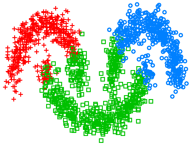
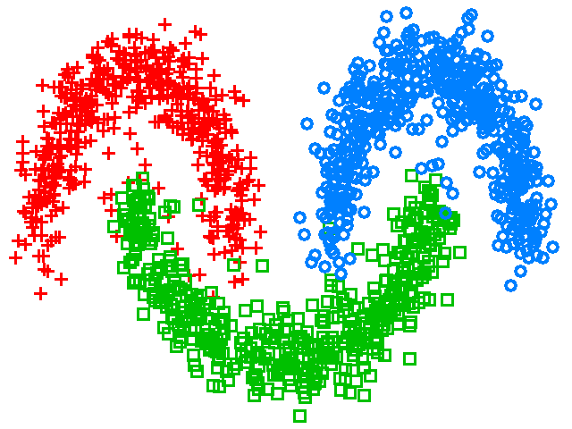
Segmentations obtained for spectral clustering and for multiclass GL with adaptive $\epsilon$ methods are shown in Fig. 3. The figure displays the best result obtained over 100 runs, corresponding to accuracies of $81.3\%$ (spectral clustering) and 97.9% (multiclass GL with adaptive $\epsilon$). The same graph structure is used for the spectral clustering decomposition and the multiclass GL method.

Figure 3: Three-moons segmentation. Left: spectral clustering. Right: multiclass GL with adaptive $\epsilon$.

(a) 100 iterations

(b) 300 iterations

(c) 1,000 iterations

(d) Energy evolution

Figure 4: Evolution of label values in three moons, using multiclass GL (fixed $\epsilon$): $\mathbb{R}^{2}$ projections at 100, 300 and 1,000 iterations, and energy evolution.

For comparison, we note the results from the literature for the simpler two-moon problem (also $\mathbb{R}^{100}$, $\sigma^{2}=0.02$ noise). The best results reported include: 94% for $p$-Laplacian [5], 95.4% for ratio-minimization relaxed Cheeger cut [25], and 97.7% for binary GL [4]. While these are not SSL methods, the last of these does involve other prior information in the form of a mass balance constraint. It can be seen that our procedures produce similarly high-quality results even for the more complex three-class segmentation problem.

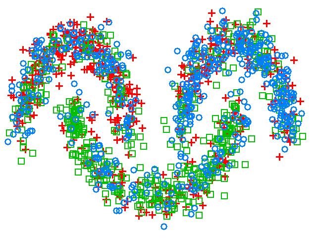
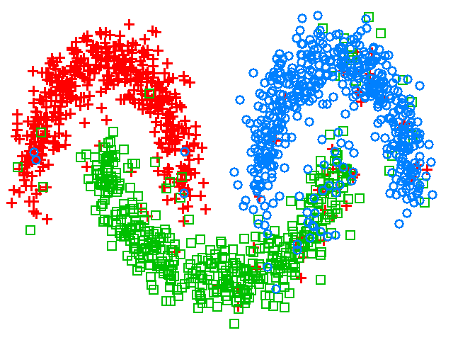
It is instructive to observe the evolution of label values in the multiclass method. Fig. 4 displays $\mathbb{R}^{2}$ projections of the results of multiclass GL (with fixed $\epsilon$), at 100, 300 and 1,000 iterations. The system starts from a random configuration. Notice that after 100 iterations, the structure is still fairly inhomogeneous, but small uniform regions begin to form. These correspond to islands around fidelity points and become seeds for further homogenization. The system progresses fast, and by 300 iterations the configuration is close to the final result: some points are still incorrectly labeled, mostly on the boundaries, but the classes form nearly uniform clusters. By 1,000 iterations the procedure converges to a steady state and a high-quality multiclass segmentation (95% accuracy) is obtained.

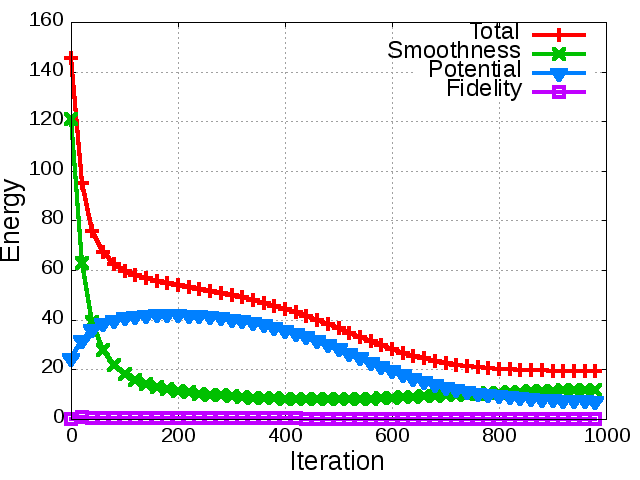
In addition, the energy evolution for one typical run is shown in Fig. 4(d) for the case with fixed $\epsilon$. The figure includes plots of the total energy (red) as well as the partial contributions of each of the three terms, namely smoothing (green), potential (blue) and fidelity (purple). Observe that at the initial iterations, the principal contribution to the energy comes from the smoothing term, but it has a fast decay due to the homogenization taking place. At the same time, the potential term increases, as $\rho$ pushes the label values toward half-integers. Eventually, the minimization process is driven by the potential term, while small local adjustments are made. The fidelity term is satisfied quickly and has almost negligible influence after the first few iterations. This picture of the “typical” energy evolution can serve as a useful guide in evaluating the performance of the method when no ground truth is available.

4.1.2 Swiss Roll.

Table 2: Swiss roll results

Method	Parameters	Correct % (stddev %)	Time [s]
$k$-means	–	37.9 (0.91)	0.05
Spectral Clustering	4 eigenvectors	49.7 (0.96)	0.05
Multiclass GL	${\mu=50}$, ${\epsilon=1}$, ${dt=0.01}$	91.0 (2.72)	0.75
	${n_{\mathrm{max}}=1,000}$

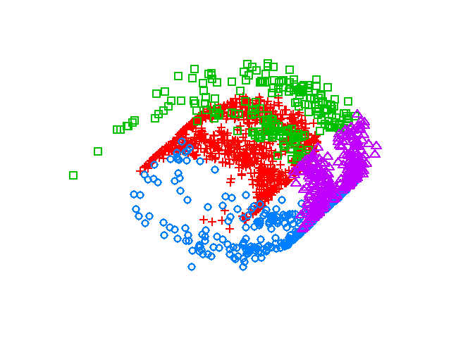
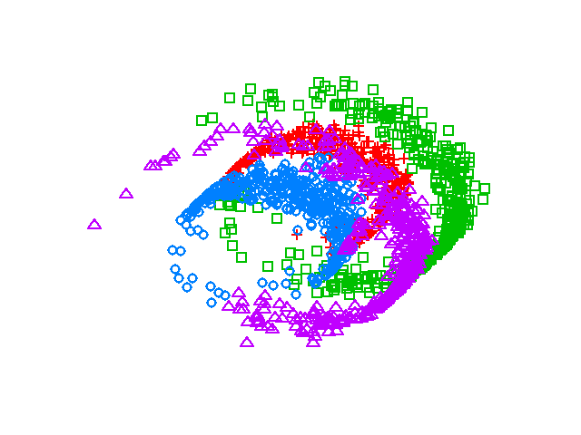
A synthetic four-class segmentation problem is constructed using the Swiss roll mapping, following the procedure in [24]. The data are created in $\mathbb{R}^{2}$ by randomly sampling from a Gaussian mixture model of four components with means at $(7.5,7.5)$, $(7.5,12.5)$, $(12.5,7.5)$ and $(12.5,12.5)$, and all covariances given by the $2\times 2$ identity matrix. 1,600 points are sampled (400 from each of the Gaussians).The data are then converted from 2 to 3 dimensions, with the following Swiss roll mapping: $(x,y)\rightarrow(x\cos(x),y,x\sin(x))$.

As before, we construct the weight matrix for a local scaling graph, with $N=10$ and scaling based on the $M=10^{th}$ closest neighbor. The fidelity set is formed by labeling $5$% of the points selected randomly.

Table 2 gives a description of the parameters used, as well as average results over 100 runs for $k$-means, spectral clustering and multiclass GL. The best results achieved over these 100 runs are shown in Fig. 5. These correspond to accuracies of $50.1\%$ (spectral clustering) and $96.4\%$ (multiclass GL). Notice that spectral clustering produces results composed of compact classes, but with a configuration that does not follow the manifold structure. In contrast, the multiclass GL method is capable of segmenting the manifold structure correctly, achieving higher accuracies.

(a) Spectral clustering

(b) Multiclass GL

Figure 5: Swiss roll results.

4.2 Image Segmentation

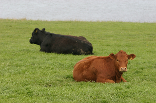
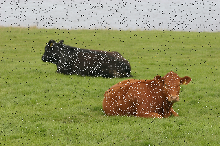
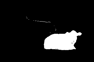
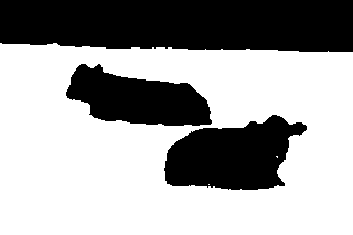
We apply our algorithm to the color image of cows shown in Fig. 6(a). This is a $213\times 320$ color image, to be divided into four classes: sky, grass, black cow and red cow. To construct the weight matrix, we use feature vectors defined as the set of intensity values in the neighborhood of a pixel. The neighborhood is a patch of size $5\times 5$. Red, green and blue channels are appended, resulting in a feature vector of dimension 75. A local scaling graph with $N=30$ and $M=30$ is constructed. For the fidelity term, 2.6% of labeled pixels are used (Fig. 6(b)).

The multiclass GL method used the following parameters: $\mu=30$, $\epsilon=1$, $dt=0.01$ and $n_{\mathrm{max}}=800$. The average time for segmentation using different fidelity sets was $19.9$ s. Results are depicted in Figs. 6(c)-6(f). Each class image shows in white the pixels identified as belonging to the class, and in black the pixels of the other classes. It can be seen that all the classes are clearly segmented. The few mistakes made are in identifying some borders of the black cow as part of the red cow, and vice-versa.

(a) Original

(b) Sampled

(c) Black cow

(d) Red cow

(e) Grass

(f) Sky

Figure 6: Color (multi-channel) image. Original image, sampled fidelity and results.

4.3 Benchmark Sets

4.3.1 COIL-100.

The Columbia object image library (COIL-100) is a set of 7,200 color images of 100 different objects taken from different angles (in steps of 5 degrees) at a resolution of $128\times 128$ pixels [22]. This image database has been preprocessed and made available by [6] as a benchmark for SSL algorithms. In summary, the red channel of each image is downsampled to $16\times 16$ pixels by averaging over blocks of $8\times 8$ pixels. Then $24$ of the objects are randomly selected and partitioned into six arbitrary classes: $38$ images are discarded from each class, leaving $250$ per class or 1,500 images in all. The downsampled $16\times 16$ images are further processed to hide the image structure by rescaling, adding noise and masking 15 of the 256 components. The result is a data set of 1,500 data points, of dimension 241.

We build a local scaling graph, with $N=4$ nearest neighbors and scaling based on the $M=4^{th}$ closest neighbor. The fidelity term is constructed by labeling $10$% of the points, selected at random. The multiclass GL method used the following parameters: $\mu=100$, $\epsilon=4$, $dt=0.02$ and $n_{\mathrm{max}}=$ 1,000. An average accuracy of 93.2%, with standard deviation of 1.27%, is obtained over 100 runs, with an average time for segmentation of $0.29$s.

For comparison, we note the results reported in [23]: 83.5% ($k$-nearest neighbors), 87.8% (LapRLS), 89.9% (sGT), 90.9% (SQ-Loss-I) and 91.1% (MP). All these are SSL methods (with the exception of $k$-nearest neighbors which is supervised), using 10% fidelity just as we do. As can be seen, our results are of greater accuracy.

4.3.2 MNIST Data.

The MNIST data set [20] is composed of 70,000 $28\times 28$ images of handwritten digits $0$ through $9$. The task is to classify each of the images into the corresponding digit. Hence, this is a $10$-class segmentation problem.

The weight matrix constructed corresponds to a local scaling graph with $N=8$ nearest neighbors and scaling based on the $M=8^{th}$ closest neighbor. We perform no preprocessing, so the graph directly uses the $28\times 28$ images. This yields a data set of 70,000 points of dimension 784. For the fidelity term, 250 images per class (2,500 images, corresponding to $3.6\%$ of the data) are chosen randomly. The multiclass GL method used the following parameters: $\mu=50$, $\epsilon=1$, $dt=0.01$ and $n_{\mathrm{max}}=$ 1,500. An average accuracy of 96.9%, with standard deviation of 0.04%, is obtained over 50 runs. The average time for segmentation using different fidelity sets was $60.89$ s.

Comparative results from other methods reported in the literature include: 87.1% (p-Laplacian [5]), 87.64% (multicut normalized 1-cut [15]), 88.2% (Cheeger cuts [25]), 92.6% (transductive classification [26]). As with the three-moon problem, some of these are based on unsupervised methods but incorporate enough prior information that they can fairly be compared with SSL methods. Comparative results from supervised methods are: 88% (linear classifiers [19, 20]), 92.3-98.74% (boosted stumps [20]), 95.0-97.17% ($k$-nearest neighbors [19, 20]), 95.3-99.65% (neural/convolutional nets [19, 20]), 96.4-96.7% (nonlinear classifiers [19, 20]), 98.75-98.82% (deep belief nets [16]) and 98.6-99.32% (SVM [19]). Note that all of these take 60,000 of the digits as a training set and 10,000 digits as a testing set [20], in comparison to our approach where we take only $3.6\%$ of the points for the fidelity term. Our SSL method is nevertheless competitive with these supervised methods. Moreover, we perform no preprocessing or initial feature extraction on the image data, unlike most of the other methods we compare with (we have excluded from the comparison, however, methods that explicitly deskew the image). While there is a computational price to be paid in forming the graph when data points use all 784 pixels as features, this is a simple one-time operation.

5 Conclusions

We have proposed a new multiclass segmentation procedure, based on the diffuse interface model. The method obtains segmentations of several classes simultaneously without using one-vs-all or alternative sequences of binary segmentations required by other multiclass methods. The local scaling method of Zelnik-Manor and Perona, used to construct the graph, constitutes a useful representation of the characteristics of the data set and is adequate to deal with high-dimensional data.

Our modified diffusion method, represented by the non-linear smoothing term introduced in the Ginzburg-Landau functional, exploits the structure of the multiclass model and is not affected by the ordering of class labels. It efficiently propagates class information that is known beforehand, as evidenced by the small proportion of fidelity points (2% – 10% of dataset) needed to perform accurate segmentations. Moreover, the method is robust to initial conditions. As long as the initialization represents all classes uniformly, different initial random configurations produce very similar results. The main limitation of the method appears to be that fidelity points must be representative of class distribution. As long as this holds, such as in the examples discussed, the long-time behavior of the solution relies less on choosing the “right” initial conditions than do other learning techniques on graphs.

State-of-the-art results with small classification errors were obtained for all classification tasks. Furthermore, the results do not depend on the particular class label assignments. Future work includes investigating the diffuse interface parameter $\epsilon$. We conjecture that the proposed functional converges (in the $\Gamma$-convergence sense) to a total variational type functional on graphs as $\epsilon$ approaches zero, but the exact nature of the limiting functional is unknown.

Acknowledgements.

This research has been supported by the Air Force Office of Scientific Research MURI grant FA9550-10-1-0569 and by ONR grant N0001411AF00002.

References

- [1] Allwein, E.L., Schapire, R.E., Singer, Y.: Reducing multiclass to binary: A unifying approach for margin classifiers. Journal of Machine Learning Research 1 (2000) 113–141
- [2] Bertozzi, A., van Gennip, Y.: Gamma-convergence of graph Ginzburg-Landau functionals. Advanced in Differential Equations 17(11–12) (2012) 1115–1180
- [3] Bertozzi, A., Esedoḡlu, S., Gillette, A.: Inpainting of binary images using the Cahn-Hilliard equation. IEEE Transactions on Image Processing 16(1) (2007) 285–291
- [4] Bertozzi, A.L., Flenner, A.: Diffuse interface models on graphs for classification of high dimensional data. Multiscale Modeling and Simulation 10(3) (2012) 1090–1118
- [5] Bühler, T., Hein, M.: Spectral clustering based on the graph -Laplacian. In Bottou, L., Littman, M., eds.: Proceedings of the 26th International Conference on Machine Learning. Omnipress, Montreal, Canada (2009) 81–88
- [6] Chapelle, O., Schölkopf, B., Zien, A., eds.: Semi-Supervised Learning. MIT Press, Cambridge, MA (2006)
- [7] Chung, F.R.K.: Spectral graph theory. In: Regional Conference Series in Mathematics. Volume 92. Conference Board of the Mathematical Sciences (CBMS), Washington, DC (1997)
- [8] Coifman, R.R., Lafon, S., Lee, A.B., Maggioni, M., Nadler, B., Warner, F., Zucker, S.W.: Geometric diffusions as a tool for harmonic analysis and structure definition of data: Diffusion maps. Proceedings of the National Academy of Sciences 102(21) (2005) 7426–7431
- [9] Dietterich, T.G., Bakiri, G.: Solving multiclass learning problems via error-correcting output codes. Journal of Artificial Intelligence Research 2(1) (1995) 263–286
- [10] Dobrosotskaya, J.A., Bertozzi, A.L.: A wavelet-Laplace variational technique for image deconvolution and inpainting. IEEE Trans. Image Process. 17(5) (2008) 657–663
- [11] Dobrosotskaya, J.A., Bertozzi, A.L.: Wavelet analogue of the Ginzburg-Landau energy and its gamma-convergence. Interfaces and Free Boundaries 12(2) (2010) 497–525
- [12] Gilboa, G., Osher, S.: Nonlocal operators with applications to image processing. Multiscale Modeling and Simulation 7(3) (2008) 1005–1028
- [13] Har-Peled, S., Roth, D., Zimak, D.: Constraint classification for multiclass classification and ranking. In S. Becker, S.T., Obermayer, K., eds.: Advances in Neural Information Processing Systems 15. MIT Press, Cambridge, MA (2003) 785–792
- [14] Hastie, T., Tibshirani, R.: Classification by pairwise coupling. In: Advances in Neural Information Processing Systems 10. MIT Press, Cambridge, MA (1998)
- [15] Hein, M., Setzer, S.: Beyond spectral clustering - tight relaxations of balanced graph cuts. In Shawe-Taylor, J., Zemel, R., Bartlett, P., Pereira, F., Weinberger, K., eds.: Advances in Neural Information Processing Systems 24. (2011) 2366–2374
- [16] Hinton, G.E., Osindero, S., Teh, Y.W.: A fast learning algorithm for deep belief nets. Neural Computation 18 (2006) 1527–1554
- [17] Jung, Y.M., Kang, S.H., Shen, J.: Multiphase image segmentation via Modica-Mortola phase transition. SIAM J. Appl. Math 67(5) (2007) 1213–1232
- [18] Kohn, R.V., Sternberg, P.: Local minimizers and singular perturbations. Proc. Roy. Soc. Edinburgh Sect. A 111(1-2) (1989) 69–84
- [19] LeCun, Y., Bottou, L., Bengio, Y., Haffner, P.: Gradient-based learning applied to document recognition. Proceedings of the IEEE 86(11) (1998) 2278–2324
- [20] LeCun, Y., Cortes, C.: The MNIST database of handwritten digits. http://yann.lecun.com/exdb/mnist/
- [21] Li, Y., Kim, J.: Multiphase image segmentation using a phase-field model. Computers and Mathematics with Applications 62 (2011) 737–745
- [22] Nene, S., Nayar, S., Murase, H.: Columbia Object Image Library (COIL-100). Technical Report CUCS-006-96 (1996)
- [23] Subramanya, A., Bilmes, J.: Semi-supervised learning with measure propagation. Journal of Machine Learning Research 12 (2011) 3311–3370
- [24] Surendran, D.: Swiss roll dataset. http://people.cs.uchicago.edu/~dinoj/manifold/ swissroll.html (2004)
- [25] Szlam, A., Bresson, X.: Total variation and cheeger cuts. In Fürnkranz, J., Joachims, T., eds.: Proceedings of the 27th International Conference on Machine Learning. Omnipress, Haifa, Israel (2010) 1039–1046
- [26] Szlam, A.D., Maggioni, M., Coifman, R.R.: Regularization on graphs with function-adapted diffusion processes. Journal of Machine Learning Research 9 (2008) 1711–1739
- [27] von Luxburg, U.: A tutorial on spectral clustering. Technical Report TR-149, Max Planck Institute for Biological Cybernetics (2006)
- [28] Wang, J., Jebara, T., Chang, S.F.: Graph transduction via alternating minimization. Proceedings of the 25th International Conference on Machine Learning (2008)
- [29] Zelnik-Manor, L., Perona, P.: Self-tuning spectral clustering. In Saul, L.K., Weiss, Y., Bottou, L., eds.: Advances in Neural Information Processing Systems 17. MIT Press, Cambridge, MA (2005)
- [30] Zhou, D., Bousquet, O., Lal, T.N., Weston, J., Schölkopf, B.: Learning with local and global consistency. In Thrun, S., Saul, L.K., Schölkopf, B., eds.: Advances in Neural Information Processing Systems 16. MIT Press, Cambridge, MA (2004) 321–328
- [31] Zhou, D., Schölkopf, B.: A regularization framework for learning from graph data. In: Workshop on Statistical Relational Learning. International Conference on Machine Learning, Banff, Canada (2004)