Stochastic Heisenberg limit: Optimal estimation of a fluctuating phase

Abstract

The ultimate limits to estimating a fluctuating phase imposed on an optical beam can be found using the recently derived continuous quantum Cramér-Rao bound. For Gaussian stationary statistics, and a phase spectrum scaling asymptotically as $\omega^{-p}$ with $p>1$, the minimum mean-square error in any (single-time) phase estimate scales as ${\cal N}^{-2(p-1)/(p+1)}$, where ${\cal N}$ is the photon flux. This gives the usual Heisenberg limit for a constant phase (as the limit $p\to\infty$) and provides a stochastic Heisenberg limit for fluctuating phases. For $p=2$ ( Brownian motion), this limit can be attained by phase tracking.

Estimating the phase imposed on an optical beam, by nature or by an agent, is a key task in metrology and communication respectively. One case of broad relevance is that where the phase varies stochastically in time over a wide range Science ; Berry02 ; Berry06 ; erratum ; Tsang ; Wheatley10 ; Iwasawa13 ; Tsang13 . It is only very recently that it has been possible to experimentally demonstrate the quantum enhancement (by a constant factor) of the estimation of such a strongly fluctuating phase, using nonclassical (squeezed) light and homodyne detection with adaptive phase tracking Science ; Iwasawa13 .

Adaptive phase tracking is a sophisticated measurement technique whereby the phase of the local oscillator (necessary for homodyne detection) is continuously changed in time to follow an estimate of the true phase Science ; Berry02 ; Berry06 ; erratum ; Tsang ; Wheatley10 ; Iwasawa13 . This enables the phase quadrature of the beam to be monitored at all times, to a good approximation, maximizing the phase information obtained. Previously it has been calculated that phase tracking with squeezed light would enable an imposed phase to be estimated with a mean square error (MSE) scaling as ${\cal N}^{-2/3}$ Berry02 ; Berry06 ; erratum . In contrast, for coherent states (no squeezing) only a ${\cal N}^{-1/2}$ scaling can be achieved Berry02 ; Berry06 ; erratum . Here ${\cal N}$ is the mean flux (photons per second) in the beam, and the imposed phase is modeled by Brownian motion.

While experiments in optical phase tracking have not yet demonstrated an improvement over the coherent state scaling of ${\cal N}^{-1/2}$, the possibility of doing so in the near future raises pressing theoretical questions: is the MSE scaling of ${\cal N}^{-2/3}$, derived assuming adaptive estimation Berry02 ; Berry06 ; erratum , the best possible? If not, what is the the ultimate limit to estimating a fluctuating phase and how can it be achieved?

For measurement of a constant phase, the fundamental bound is the Heisenberg limit heislim ; WisMil10 : a phase estimate MSE scaling as $\langle N\rangle^{-2}$, where $\langle N\rangle$ is the mean number of photons per estimate. This a quadratic improvement over the $\langle N\rangle^{-1}$ scaling achievable using coherent states (the standard quantum limit, or SQL) heislim ; WisMil10 . Hence, if quantum mechanics similarly allowed a quadratic improvement in the case of a fluctuating phase, the corresponding fundamental limit for the MSE would scale as ${\cal N}^{-1}$.

Contrary to this intuition, we prove in this paper, with only weak assumptions, that the fundamental bound to estimating Brownian phase fluctuations is a MSE scaling as ${\cal N}^{-2/3}$. This establishes that adaptive phase tracking can be a very effective measurement technique for this problem, giving an uncertainty at most a constant factor greater than the minimum allowed by quantum mechanics (under our assumptions). This ${\cal N}^{-2/3}$ scaling for Brownian fluctuations is just a special case of our general stochastic Heisenberg limit, which allows for any inverse power-law describing the phase fluctuation spectrum at high frequencies, and which also yields the constant-phase Heisenberg limit as a special case.

This paper is organised as follows. First we derive the general stochastic Heisenberg limit, and the stochastic SQL. Next we specialize to the scenario of Ref. Science : a squeezed beam comprising the output of an optical parametric oscillator (OPO) with an added mean field, and a phase varying like damped Brownian motion. We consider the ultimate limit, and find the same scaling as in the general case, but with an explicit constant of proportionality, consistent with the numerics of Ref. erratum .

I General proof

Our result applies to the situation of a continuous beam [a one-dimensional quantum field ${b}(t)$], on which there is an imposed phase $\varphi(t)$. We require only three conditions:

1. The statistics of the field quadratures and imposed phase are stationary.

2. The statistics of the field quadratures and imposed phase are Gaussian and time-symmetric.

3. The phase spectrum scales as $|\omega|^{-p}$ for large $|\omega|$, for some $p>1$.

We now explain these conditions in more detail. The instantaneous creation operator $b^{\dagger}(t)$ of the beam obeys $[b(t),b^{\dagger}(t^{\prime})]=\delta(t-t^{\prime})$, and $\langle b^{\dagger}(t)b(t)\rangle={\cal N}$ is the photon flux WisMil10 . The stationarity of its statistics, and those of $\varphi(t)$, means that one-time expectation values are constant, and two-time correlations depend only on the time difference.

The assumed Gaussian statistics mean there is a Gaussian Wigner functional for the quadratures WisMil10

$$X(t):=b^{\dagger}(t)+b(t),\qquad Y(t):=i[b^{\dagger}(t)-b(t)],$$ (1)

and a Gaussian distribution for the phase $\varphi(t)$. For a single Gaussian variable, such as $\varphi(t)$, the autocorrelation function is automatically time-symmetric. However, the beam quadratures $X(t)$ and $Y(t^{\prime})$ may be correlated, and our derivation below requires that this cross-correlation be time-symmetric (i.e. invariant under $t\leftrightarrow t^{\prime}$).

The third condition allows for a vast range of phase fluctuation models. For $p=2$ it means that at short times the fluctuations are like Wiener noise WisMil10 (Brownian motion), which has the spectrum $\kappa/\omega^{2}$, where $\kappa$ is a constant with units of frequency. More generally, we take the scaling constant to be $\kappa^{p-1}$, so $\kappa$ still has units of frequency. In the limit $p\to\infty$ the phase is effectively constant.

In Ref. TsangWise , a continuous form of the quantum Cramér-Rao inequality was derived, giving a lower bound on the MSE of any unbiased estimate, $\hat{\varphi}(t)$, of a time-varying parameter $\varphi(t)$,

$$\langle[\hat{\varphi}(t)-\varphi(t)]^{2}\rangle\geq F^{-1}(t,t).$$ (2)

Here $F(t,t^{\prime})$ is the Fisher information matrix (with continuous indices $t$ and $t^{\prime}$) of the phase of the beam, given by a sum of quantum and classical contributions

$$F(t,t^{\prime}):=F^{(Q)}(t,t^{\prime})+F^{(C)}(t,t^{\prime}),$$ (3)

and the (matrix) inverse in Eq. (2) is defined by

$$\int ds\,F^{-1}(t,s)F(s,t^{\prime})=\delta(t-t^{\prime}).$$ (4)

For the case where $\varphi(t)$ is an imposed phase,

$$F^{(Q)}(t,t^{\prime}) :=4\left\langle\Delta n(t)\Delta n(t^{\prime})\right\rangle,$$ (5)

$$F^{(C)}(t,t^{\prime}) :=\int D\varphi\,P[\varphi]\frac{\delta\,\ln P[\varphi]}{\delta\varphi(t)}\frac{\delta\,\ln P[\varphi]}{\delta\varphi(t^{\prime})}.$$ (6)

In the above, $\int D\varphi\,\cdots$ denotes an integral over all possible functions $\varphi(t)$, the functional $P[\varphi]$ gives the prior weight for each function, and $\delta/\delta\varphi(t)$ is a functional derivative. Also, $\Delta n(t)=n(t)-\langle n(t)\rangle$, where $n(t):=b^{\dagger}(t)b(t)$ is the generator of the phase shifts, the photon flux operator. Because of the stationarity condition, all quantities dependent on two times $t$ and $t^{\prime}$ are functions only of $t-t^{\prime}$. We will express these quantities explicitly as functions of $t-t^{\prime}$ from here on. In particular, the lower bound in Eq. (2) will be denoted by $F^{-1}(0)$.

To determine $F^{-1}(0)$, substitute Eq. (3) into Eq. (4) and take the Fourier transform, to give

$$\tilde{F}^{-1}(\omega)=\frac{1}{\tilde{F}^{(C)}(\omega)+\tilde{F}^{(Q)}(\omega)},$$ (7)

for the Fourier transform of $F^{-1}(t-t^{\prime})$. The value of $F^{-1}(0)$ is then obtained by integrating this over $\omega$. Our aim is to determine the minimum possible scaling of this value with the photon flux ${\cal N}=\langle n(t)\rangle$.

As we assume the phase fluctuations are Gaussian, we have $F^{(C)}(t-t^{\prime})=\Sigma^{-1}(t-t^{\prime})$, with $\Sigma(t-t^{\prime}):=\langle\varphi(t)\varphi(t^{\prime})\rangle-\langle\varphi\rangle^{2}$ Hall02 . For the case $\tilde{\Sigma}(\omega)=\kappa^{p-1}/|\omega|^{p}$,

$$\tilde{F}^{-1}(\omega)=\frac{\kappa^{p-1}}{|\omega|^{p}+\kappa^{p-1}\tilde{F}^{(Q)}(\omega)}.$$ (8)

More generally, we can obtain the result below with the weaker requirement that the phase spectrum approaches this scaling at high frequencies, i.e., $\tilde{\Sigma}(\omega)=\Omega(\kappa^{p-1}/|\omega|^{p})$ as per condition 3 (see Appendix D).

Next we consider the quantity $F^{(Q)}(t-t^{\prime})$; this may be simplified to (see Appendix A)

$$F^{(Q)}(t-t^{\prime})=4{\cal N}\delta(t-t^{\prime})+f(t-t^{\prime})-g(t-t^{\prime}),$$ (9)

where, in terms of the quadrature operators (1),

$$f(t-t^{\prime}) :=\frac{1}{2}\left[\langle:X(t)X(t^{\prime}):\rangle+\langle:Y(t)Y(t^{\prime}):\rangle\right]^{2}$$ (10)

$$g(t-t^{\prime}) :=\langle:X(t)X(t^{\prime}):\rangle\langle:Y(t)Y(t^{\prime}):\rangle$$

$$\quad-\frac{1}{2}\left(\langle:X(t)Y(t^{\prime}):\rangle^{2}+\langle:Y(t)X(t^{\prime}):\rangle^{2}\right)$$

$$\quad+\frac{1}{2}\left(\langle X\rangle^{2}+\langle Y\rangle^{2}\right)^{2}.$$ (11)

Thus, from Eq. (8), we obtain

$$\tilde{F}^{-1}(\omega)=\frac{\kappa^{p-1}}{|\omega|^{p}+\kappa^{p-1}\left[4{\cal N}+\tilde{f}(\omega)-\tilde{g}(\omega)\right]}.$$ (12)

The photon flux can be written as

$${\cal N}=\frac{1}{4}\left(\langle:X(t)X(t):\rangle+\langle:Y(t)Y(t):\rangle\right),$$ (13)

and therefore $f(0)=8{\cal N}^{2}$. In addition, using a spectral uncertainty principle and the assumption of time-symmetric correlations, it can be shown that ${\cal N}/4\geq-\tilde{g}(\omega)$ and $\tilde{f}(\omega)\geq 0$ (see Appendix B). Since it is easily shown that $F^{(Q)}(t-t^{\prime})$ is a positive-definite function, by Bochner’s theorem $\tilde{F}^{(Q)}(\omega)\geq 0$ pos , and thus the denominator in Eq. (12) is positive. Consequently, replacing $-\tilde{g}(\omega)$ with ${\cal N}/4$ can only decrease the right-hand side; that is, with $\zeta=17/4$,

$$\tilde{F}^{-1}(\omega)\geq\frac{\kappa^{p-1}}{|\omega|^{p}+\kappa^{p-1}\left[\zeta{\cal N}+\tilde{f}(\omega)\right]}.$$ (14)

Next, from the fact that $f(0)=8{\cal N}^{2}$, the integral of $\tilde{f}(\omega)$ is ${\cal I}=16\pi{\cal N}^{2}$. This means that $\tilde{f}(\omega)$ cannot be larger than $\mu$ over a range greater than ${\cal I}/\mu$. To place a lower bound on $F^{-1}(0)$, when integrating Eq. (14) we may first omit the range of integration where $\tilde{f}(\omega)>\mu$, and replace $\tilde{f}(\omega)$ by $\mu$ over the remaining portion. Second, we can assume that the range of integration omitted is for the smallest values of $\omega$ because that can only further reduce the value of the integral. Since this range can be at most ${\cal I}/\mu$ in length, this yields

$$F^{-1}(0) \geq\frac{1}{\pi}\int_{{\cal I}/2\mu}^{\infty}\frac{\kappa^{p-1}\,d\omega}{\omega^{p}+\kappa^{p-1}\left(\zeta{\cal N}+\mu\right)}$$

$$\geq\frac{1}{2\pi}\int_{0}^{\infty}\frac{\kappa^{p-1}\,d\omega}{\omega^{p}+\kappa^{p-1}\left(\zeta{\cal N}+\mu\right)}$$

$$\geq\frac{\kappa^{p-1}}{2\pi[\kappa^{p-1}(\zeta{\cal N}+\mu)]^{1-1/p}},$$ (15)

where the inequality on the second line holds for $({\cal I}/\mu)^{p}\leq\kappa^{p-1}\left(\zeta{\cal N}+\mu\right)$ (see Appendix C).

To obtain the strongest lower bound on $F^{-1}(0)$ we consider the smallest value of $\mu$ that we can take such that $({\cal I}/\mu)^{p}\leq\kappa^{p-1}\left(\zeta{\cal N}+\mu\right)$. This value is $\mu=\Theta({\cal N}({\cal N}/\kappa)^{(p-1)/(p+1)})$. We consider scaling for large ${\cal N}/\kappa$, in which case $\mu\gg{\cal N}$, and $\zeta{\cal N}$ can be ignored. Equations (2) and (I) thus yield our main result, the lower bound scaling for the MSE,

$$\langle[\hat{\varphi}(t)-\varphi(t)]^{2}\rangle=\Omega\left(\left({\kappa}/{{\cal N}}\right)^{2(p-1)/(p+1)}\right).$$ (16)

Note this scaling cannot be achieved by a coherent-state beam, for which $F^{(Q)}(t-t^{\prime})=4{\cal N}\delta(t-t^{\prime})$. It is easy to show, for this case, by taking $f=g=0$ in Eq. (12), that

$$\langle[\hat{\varphi}(t)-\varphi(t)]^{2}\rangle_{\rm SQL}=\Omega\left(\left({\kappa}/{{\cal N}}\right)^{(p-1)/p}\right).$$ (17)

which we call the stochastic SQL scaling.

In the case of Wiener phase fluctuations ($p=2$), the stochastic Heisenberg scaling is $(\kappa/{\cal N})^{2/3}$. A simplified analysis in Ref. Berry02 found that adaptive homodyne measurements can yield this scaling, but it took into account neither the photon flux due to the squeezing nor the information in the photocurrent noise. A more complete analysis, taking both of these terms into account, was performed in Ref. erratum (correcting an error in the analysis of Ref. Berry06 ). This verified this scaling of $(\kappa/{\cal N})^{2/3}$ for the MSE. That is, the lower bound in Eq. (16) is attainable by adaptive measurements for $p=2$.

The limit $p\to\infty$ gives a very slowly varying phase. In that case Eq. (16) gives the expected constant-phase Heisenberg limit scaling $\langle[\hat{\varphi}(t)-\varphi(t)]^{2}\rangle=\Omega(\langle{\cal N}\rangle^{-2})$. Similarly, Eq. (17) gives the expected SQL scaling $\langle[\hat{\varphi}(t)-\varphi(t)]^{2}\rangle_{\rm SQL}=\Omega(\langle{\cal N}\rangle^{-1})$. For all other $p$, the quantum enhancement is less than quadratic, and as $p\to 1$ there is no quantum advantage.

II OPO squeezing and OU fluctuations

Next we specialise to the model of squeezing used in Refs. Science ; Berry02 ; Berry06 —a coherent field of real amplitude $\alpha$ added to an Optical Parametric Oscillator (OPO) output—and to phase fluctuations modeled by Ornstein-Uhlenbeck (OU) noise, with $\tilde{\Sigma}(\omega)=\kappa/(\lambda^{2}+\omega^{2})$ as in Ref. Science . Asymptotically this is identical to the Wiener phase spectrum $(p=2)$ analysed above. For this beam we have $\langle X\rangle=2\alpha$, $\langle Y\rangle=0$, so Eq. (9) becomes

$$F^{(Q)}(t-t^{\prime}) =4{\cal N}\delta(t-t^{\prime})+4\alpha^{2}T_{+}(t-t^{\prime})$$

$$\quad+\left\{[T_{+}(t-t^{\prime})]^{2}+[T_{-}(t-t^{\prime})]^{2}\right\}/2,$$ (18)

where $T_{\pm}(t-t^{\prime})$ are the normally ordered correlation functions for the quadrature fluctuations Science ; c17

$$T_{\pm}(t-t^{\prime})=\langle:\Delta Q_{\pm}(t)\Delta Q_{\pm}(t^{\prime}):\rangle,$$ (19)

where $Q_{+}:=X$ and $Q_{-}:=Y$. They are given by

$$T_{\pm}(t-t^{\prime})=(R_{\pm}-1)\frac{(1\mp x)\gamma}{4}e^{-(1\mp x)\gamma|t-t^{\prime}|/2}.$$ (20)

In Eq. (20), $R_{\pm}$ are the antisqueezing and squeezing levels, respectively, at the center frequency. For an OPO, $\gamma$ is the cavity’s decay rate c18 and $x\in[0,1)$ is the normalized pump amplitude. In terms of these quantities, the total photon flux is

$${\cal N}=\alpha^{2}+\frac{\gamma}{16}[(R_{+}-1)(1-x)+(R_{-}-1)(1+x)].$$ (21)

Substituting these expressions in Eq. (18) and taking the Fourier transform yields

$$\tilde{F}^{(Q)}(\omega)=4{\cal N}+4\alpha^{2}(R_{+}-1)\frac{(1-x)^{2}\gamma^{2}}{(1-x)^{2}\gamma^{2}+4\omega^{2}}$$

$$+\frac{\gamma^{3}}{16}\left[\frac{(R_{+}-1)^{2}(1-x)^{3}}{(1-x)^{2}\gamma^{2}+\omega^{2}}+\frac{(R_{-}-1)^{2}(1+x)^{3}}{(1+x)^{2}\gamma^{2}+\omega^{2}}\right].$$ (22)

For a coherent state ($R_{+}=R_{-}=1$), we would just have $\tilde{F}^{(Q)}(\omega)=4{\cal N}$, and we would obtain $\kappa/(2\sqrt{4{\cal N}\kappa+\lambda^{2}})$ as the lower bound on the MSE. This coherent state limit was first derived by Tsang et al. (see Eq. (4.5) in Ref. Tsang ) and scales asymptotically as $(\kappa/{\cal N})^{1/2}$ as expected Berry02 .

II.1 Comparison with the Science experiment

It seems impossible to obtain an exact analytical solution for $F^{-1}(0)$ in the case of general OPO squeezing. However, a useful approximation is to just include the terms in Eq. (22) that represent information available from the mean field; that is, those terms proportional to $\alpha^{2}$. As in the theory of Ref. Berry02 , the estimation performed in Ref. Science only used the signal from the mean field, so this approximation is relevant to those works. As in those works we also express our results in terms of $\alpha^{2}$, rather than ${\cal N}$. Then we find

$$F^{-1}(0)=\frac{(\kappa/2)\left(1+g^{2}/\sqrt{\Xi_{+}\Xi_{-}}\right)}{\sqrt{\Xi_{+}}+\sqrt{\Xi_{-}}},$$ (23)

where

$$\Xi_{\pm}=\frac{1}{2}\left(4\alpha^{2}\kappa+\lambda^{2}+g^{2}\pm\sqrt{(4\alpha^{2}\kappa+\lambda^{2}-g^{2})^{2}-4d}\right),$$ (24)

with $g=(1-x)\gamma/2$ and $d=4\kappa\alpha^{2}(R_{+}-1)g^{2}$.

With further simplification this bound on the MSE is comparable to the results given for adaptive measurements on squeezed states in Ref. Science . First we note that a mixed squeezed state described by $R_{\pm}$, $\gamma$ and $x$ can be assumed to be a combination of a pure squeezed state and classical amplitude noise (see Appendix E), where the pure squeezed state is described by $R_{-}^{Q}=R_{-}$, $R_{+}^{Q}=1/R_{-}$, $x^{Q}=(\sqrt{R_{+}}-1)/(\sqrt{R_{+}}+1)$, and $\gamma^{Q}=\gamma(1+x)/(1+x^{Q})$. Then one can determine $F^{(Q)}$ from the parameters for the pure squeezed state.

Using this approach, in the limit of large bandwidth, $\gamma\to\infty$, we obtain $\kappa/(2\sqrt{4\alpha^{2}R_{-}\kappa+\lambda^{2}})$ as the lower bound on the MSE. This expression is that shown as trace (iii) in Fig. 3 of Ref. Science , derived from Eq. (3) of Ref. Science by taking $\sigma_{f}\to 0$ (the limit of perfectly accurate feedback). Note that this is significantly below what was observed in the experiment, because the mean-field adaptive algorithm used in the experiment was far from being perfectly accurate.

II.2 Ultimate limit for OPO squeezing and $p=2$

We have already shown that the lower bound to the MSE for $p=2$ scales as $(\kappa/{\cal N})^{2/3}$. Now we show how to determine the constant of the scaling for this model assuming ideal OPO squeezing with $R_{-}=1/R_{+}$. We include all terms in Eq. (22) and express our results in terms of ${\cal N}$. We introduce dimensionless (starred) parameters via ${\cal N}=\kappa{\cal N}_{\star}$, $\alpha^{2}=\alpha_{\star}^{2}\kappa{\cal N}_{\star}$, $\gamma=\gamma_{\star}\kappa{\cal N}_{\star}^{5/6}$, $R_{+}=R_{\star}{\cal N}_{\star}^{1/3}$, and $\omega=\omega_{\star}\kappa{\cal N}_{\star}^{2/3}$, where $\gamma_{\star}>0$ and $R_{\star}>0$. Then we obtain in the limit ${\cal N}_{\star}\to\infty$ (see Appendix F)

$$F^{-1}(0)={{\cal N}_{\star}}^{-2/3}\frac{1}{2\pi}\int_{-\infty}^{\infty}\frac{d\omega_{\star}}{\omega_{\star}^{2}+\tilde{F}_{\star}^{(Q)}(\omega_{\star})},$$ (25)

with

$$\tilde{F}_{\star}^{(Q)}(\omega_{\star}) =\frac{4\gamma_{\star}^{2}\alpha_{\star}^{2}}{\gamma_{\star}^{2}/R_{\star}+\omega_{\star}^{2}}+\frac{\gamma_{\star}^{3}\sqrt{R_{\star}}/2}{4\gamma_{\star}^{2}/R_{\star}+\omega_{\star}^{2}}.$$ (26)

From Eq. (21), the above dimensionless parameters are related by $\alpha_{\star}^{2}=1-\gamma_{\star}\sqrt{R_{\star}}/8$. It is convenient to define $\tau=\gamma_{\star}\sqrt{R_{\star}}/8$, so the allowable values for $\tau$ range from $0$ to $1$. The value of $C:={{\cal N}_{\star}}^{2/3}F^{-1}(0)$ was calculated for this range of $\tau$, and $\gamma_{\star}\in[0,4]$; the results are given in Fig. 1. It can be seen that $C$ is smallest for $\tau=1$, which corresponds to a squeezed vacuum, and the minimum is $C_{0}=(587-143\sqrt{13})^{1/6}/(4\sqrt{6})\approx 0.20788$ for $\gamma_{\star}=2[2(\sqrt{13}-3)]^{1/3}\approx 2.1319$. That is,

$$\langle[\hat{\varphi}(t)-\varphi(t)]^{2}\rangle\gtrsim C_{0}\left(\kappa/{\cal N}\right)^{2/3},$$ (27)

with $C_{0}\approx 0.20788$. In this limit of a squeezed vacuum it is only possible to obtain the estimate of the phase modulo $\pi$. However, the shallowness of the plot with $\tau$ shows that one can obtain close to the optimal value for large coherent amplitude, so the phase can be measured modulo $2\pi$. The phase tracking simulations in Ref. erratum showed that it is possible to estimate $\varphi$ modulo $2\pi$ with $\langle[\hat{\varphi}(t)-\varphi(t)]^{2}\rangle\approx\left(\kappa/{\cal N}\right)^{2/3}$. Moreover those simulations obtained $\hat{\varphi}(t)$ by filtering the data prior to $t$. By using smoothing Tsang09 of the data before and after $t$, one would halve this MSE Science ; Tsang ; Wheatley10 ; Iwasawa13 .

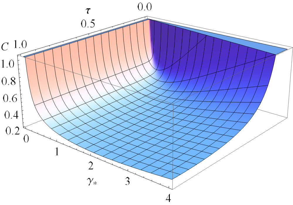
Figure 1: Plot of $C$ as a function of $\gamma_{\star}$ and $\tau$ (all dimensionless).

III Conclusion

In summary, we have found a stochastic form of the Heisenberg limit for measurements of a fluctuating phase imposed on a beam with time-invariant statistics. For Wiener fluctuations, the scaling of $(\kappa/{\cal N})^{2/3}$ is tight, in that there is a known adaptive measurement scheme that achieves it. Our bound also reproduces the (tight) Heisenberg scaling of $(\kappa/{\cal N})^{-1}$ for an effectively constant phase. We thus conjecture our general bound to be tight for all power-law phase spectra. We do note, however, that we have assumed a beam with time-symmetric Gaussian statistics, and it is an interesting open question to prove (or disprove) our bound without this assumption.

Supplemental Material

IV A: Simplifying the Fisher information for Gaussian states

Here we show how to obtain Eq. (9) from (5) in the paper. To evaluate averages such as $\langle X^{2}(t)X^{2}(t^{\prime})\rangle$, note that the operators for the different times commute, so this is the same as a symmetrically ordered moment, and we can use the Wigner function. This means that the expectation values will satisfy the same rules as for probability distributions.

For Gaussian distributions, one finds that

$$\langle x_{1}^{2}x_{2}^{2}\rangle-\langle x_{1}^{2}\rangle\langle x_{2}^{2}\rangle=2(\langle x_{1}x_{2}\rangle^{2}-\bar{x}_{1}^{2}\bar{x}_{2}^{2}).$$ (S1)

As a result,

$$\langle Q_{\pm}^{2}(t)Q_{\pm}^{2}(t^{\prime})\rangle =\langle Q_{\pm}^{2}\rangle\langle Q_{\pm}^{2}\rangle+2\langle Q_{\pm}(t)Q_{\pm}(t^{\prime})\rangle^{2}$$

$$\quad-2\langle Q_{\pm}\rangle^{2}\langle Q_{\pm}\rangle^{2},$$ (S2)

where $Q_{+}:=X$ and $Q_{-}:=Y$. Note that for expectation values at a single time, we can omit the time-dependence due to stationarity. For $t\neq t^{\prime}$, $X(t)$ and $Y(t^{\prime})$ commute, so we can again use the Wigner function to take the average, giving

$$\langle X^{2}(t)Y^{2}(t^{\prime})\rangle =\langle X^{2}\rangle\langle Y^{2}\rangle+2\langle X(t)Y(t^{\prime})\rangle^{2}$$

$$\quad-2\langle X\rangle^{2}\langle Y\rangle^{2}.$$ (S3)

On the other hand, to include the case $t=t^{\prime}$, we need to explicitly symmetrise. This is not needed for $\langle X^{2}(t)X^{2}(t^{\prime})\rangle$, because it is already symmetric, but it is needed for $\langle X^{2}(t)Y^{2}(t^{\prime})\rangle$.

Using the commutation relation $[X(t),Y(t^{\prime})]=2i\delta(t-t^{\prime})$ enables us to evaluate the symmetrised form

$$\big{\langle}X^{2}(t)Y^{2}(t^{\prime})\big{\rangle}_{S}=\big{\langle}X^{2}(t)Y^{2}(t^{\prime})\big{\rangle}$$

$$-4i\delta(t-t^{\prime})\big{\langle}X(t)Y(t^{\prime})\big{\rangle}-2\delta^{2}(t-t^{\prime}).$$ (S4)

The subscript $S$ indicates the expectation value of the symmetrically ordered operator. We then obtain

$$\langle X^{2}(t)Y^{2}(t^{\prime})\rangle =\langle X^{2}(t)Y^{2}(t^{\prime})\rangle_{S}+4i\delta(t-t^{\prime})\langle X(t)Y(t^{\prime})\rangle$$

$$\quad+2\delta^{2}(t-t^{\prime}).$$ (S5)

Similarly we obtain

$$\langle Y^{2}(t)X^{2}(t^{\prime})\rangle =\langle Y^{2}(t)X^{2}(t^{\prime})\rangle_{S}-4i\delta(t-t^{\prime})\langle Y(t)X(t^{\prime})\rangle$$

$$\quad+2\delta^{2}(t-t^{\prime}).$$ (S6)

Then we get

$$\langle X^{2}(t)Y^{2}(t^{\prime})\rangle_{S} =\langle X^{2}\rangle\langle Y^{2}\rangle+2\langle X(t)Y(t^{\prime})\rangle_{S}^{2}$$

$$\quad-2\langle X\rangle^{2}\langle Y\rangle^{2}$$

$$=\langle X^{2}\rangle\langle Y^{2}\rangle+2\langle X(t)Y(t^{\prime})\rangle^{2}$$

$$\quad-4i\delta(t-t^{\prime})\langle X(t)Y(t^{\prime})\rangle-2\delta^{2}(t-t^{\prime})$$

$$\quad-2\langle X\rangle^{2}\langle Y\rangle^{2},$$ (S7)

and so the delta functions cancel out to give Eq. (IV) even for $t=t^{\prime}$. Similarly

$$\langle Y^{2}(t)X^{2}(t^{\prime})\rangle =\langle Y^{2}\rangle\langle X^{2}\rangle+2\langle Y(t)X(t^{\prime})\rangle^{2}$$

$$\quad-2\langle Y\rangle^{2}\langle X\rangle^{2},$$ (S8)

both for $t=t^{\prime}$ and for $t\neq t^{\prime}$.

We can write Eq. (5) in the form

$$F^{(Q)}(t-t^{\prime}) =4\left[{\rm Re}\langle b^{\dagger}(t)b(t)b^{\dagger}(t^{\prime})b(t^{\prime})\rangle\right.$$

$$\quad\left.-\langle b^{\dagger}(t)b(t)\rangle\langle b^{\dagger}(t^{\prime})b(t^{\prime})\rangle\right]$$

$$=\frac{1}{4}\langle[X^{2}(t)+Y^{2}(t)][X^{2}(t^{\prime})+Y^{2}(t^{\prime})]\rangle$$

$$\quad-\frac{1}{4}\langle X^{2}+Y^{2}\rangle^{2}.$$ (S9)

Using the above results for Gaussian states, Eqs. (IV), (IV), (IV), this becomes

$$F^{(Q)}(t,t^{\prime})=\frac{1}{2}\left[\langle X(t)X(t^{\prime})\rangle^{2}+\langle Y(t)Y(t^{\prime})\rangle^{2}\right.$$

$$\left.+\langle X(t)Y(t^{\prime})\rangle^{2}+\langle Y(t)X(t^{\prime})\rangle^{2}-\left(\langle X\rangle^{2}+\langle Y\rangle^{2}\right)^{2}\right].$$ (S10)

Changing to the normally ordered form we obtain

$$F^{(Q)}(t,t^{\prime}) =4{\cal N}\delta(t-t^{\prime})-\frac{1}{2}\left(\langle X\rangle^{2}+\langle Y\rangle^{2}\right)^{2}$$

$$\quad+\frac{1}{2}\left[\langle:X(t)X(t^{\prime}):\rangle^{2}+\langle:Y(t)Y(t^{\prime}):\rangle^{2}\right.$$

$$\quad\left.+\langle:X(t)Y(t^{\prime}):\rangle^{2}+\langle:Y(t)X(t^{\prime}):\rangle^{2}\right].$$ (S11)

Using the functions $f$ and $g$, Eq. (IV) simplifies to Eq. (9) in the paper.

V B: Bounding $\tilde{g}(\omega)$ and $\tilde{f}(\omega)$

Let us define the 2-vector $Z(t)$, $2\times 2$ Hermitian matrix function $M(t,t^{\prime})$, and symmetrised correlation function $S_{AB}(t,t^{\prime})$ by

$$Z(t) :=\left(\begin{array}[]{c}X(t)\\ Y(t)\end{array}\right),$$ (S14)

$$M(t,t^{\prime}) :=\langle Z(t)Z^{\dagger}(t^{\prime})+Z(t^{\prime})Z^{\dagger}(t)\rangle/2,$$

$$S_{AB}(t,t^{\prime}) :=\langle A(t)B(t^{\prime})+B(t^{\prime})A(t)+A(t^{\prime})B(t)$$

$$\qquad+B(t)A(t^{\prime})\rangle/4.$$ (S15)

Using the commutation relation $[X(t),Y(t^{\prime})]=2i\delta(t-t^{\prime})$, one can write $M$ in the form

$$M=\left(\begin{array}[]{cc}S_{XX}&S_{XY}+i\openone\\ S_{XY}-i\openone&S_{YY}\end{array}\right),$$ (S16)

where $\openone(t,t^{\prime}):=\delta(t-t^{\prime})$. Note that $M(t,t^{\prime})$ is positive definite, in the sense that

$$\int dt\,dt^{\prime}\,\xi(t)M(t,t^{\prime})\xi^{\dagger}(t^{\prime})=\langle\aleph_{1}\aleph_{1}^{\dagger}+\aleph_{2}\aleph_{2}^{\dagger}\rangle/2\geq 0$$ (S17)

for any 2-vector function $\xi(t)$, with $\aleph_{1}:=\int dt\,\xi(t)Z(t)$ and $\aleph_{2}:=\int dt\,\xi^{\dagger}(t)Z(t)$ (this is the continuous analog of the Schrödinger-Robertson multimode uncertainty relation simon ). Stationarity implies further that $M(t,t^{\prime})$ can be written as $M(t-t^{\prime})$. Hence, taking Fourier transforms, Eq. (S17) is equivalent to the property

$$\int d\omega\,\tilde{\xi}(\omega)\tilde{M}(\omega)\tilde{\xi}^{\dagger}(\omega)\geq 0$$ (S18)

for all 2-vector functions $\tilde{\xi}(\omega)$, implying that the $2\times 2$ matrix $\tilde{M}$ is positive; i.e., that

$$\left(\begin{array}[]{cc}\tilde{S}_{XX}&\tilde{S}_{XY}+i\\ \tilde{S}_{YX}-i&\tilde{S}_{YY}\end{array}\right)\geq 0$$ (S19)

(a two-dimensional form of Bochner’s theorem pos ). This can equivalently be written as the three inequalities $\tilde{S}_{XX}(\omega)\geq 0$, $\tilde{S}_{YY}(\omega)\geq 0$, and the spectral uncertainty principle

$$\tilde{S}_{XX}(\omega)\tilde{S}_{YY}(\omega)\geq[\tilde{S}_{XY}(\omega)]^{2}+1.$$ (S20)

Note that $S_{XX}$, $S_{YY}$, and $S_{XY}$ are time symmetric by construction, and so have real Fourier transforms.

Let us further define

$$g^{a}(t-t^{\prime}) :=\langle:X(t)X(t^{\prime}):\rangle\langle:Y(t)Y(t^{\prime}):\rangle$$

$$g^{b}(t-t^{\prime}) :=-\frac{1}{2}\left(\langle:X(t)Y(t^{\prime}):\rangle^{2}+\langle:Y(t)X(t^{\prime}):\rangle^{2}\right)$$

$$g^{c}(t-t^{\prime}) :=\frac{1}{2}\left(\langle X\rangle^{2}+\langle Y\rangle^{2}\right)^{2},$$ (S21)

so from Eq. (11) of the paper, $g(t-t^{\prime})=g^{a}(t-t^{\prime})+g^{b}(t-t^{\prime})+g^{c}(t-t^{\prime})$. Our first aim is to bound $\tilde{g}(\omega)$ in terms of ${\cal N}$ using the inequality in Eq. (S20).

The inequality (S20) means that

$$[1+\tilde{h}_{X}(\omega)][1+\tilde{h}_{Y}(\omega)]\geq[\tilde{h}_{XY}(\omega)]^{2}+1,$$ (S22)

where

$$h_{X}(t-t^{\prime}) :=\langle:X(t)X(t^{\prime}):\rangle$$

$$h_{Y}(t-t^{\prime}) :=\langle:Y(t)Y(t^{\prime}):\rangle$$

$$h_{XY}(t-t^{\prime}) :=\frac{1}{2}\left[\langle:X(t)Y(t^{\prime})+Y(t)X(t^{\prime}):\rangle\right].$$ (S23)

Because $h_{X}$, $h_{Y}$, and $h_{XY}$ are time symmetric by construction, $\tilde{h}_{X}$, $\tilde{h}_{Y}$ and $\tilde{h}_{XY}$ are real. Further, the assumption in the paper that the cross-correlation between the quadratures is time symmetric, i.e., that the symmetrized (or Wigner) cross-correlations satisfy $\frac{1}{2}\langle X(t)Y(t^{\prime})+Y(t^{\prime})X(t)\rangle=\frac{1}{2}\langle X(t^{\prime})Y(t)+Y(t)X(t^{\prime})\rangle$, is equivalent to $\langle:X(t)Y(t^{\prime}):\rangle=\langle:X(t^{\prime})Y(t):\rangle$, implying

$$h_{XY}(t-t^{\prime})=\langle:X(t)Y(t^{\prime}):\rangle.$$ (S24)

Using the above relations, we can write the photon flux as

$${\cal N} =\frac{2}{\pi}\int d\nu\left[\tilde{h}_{X}(\nu)+\tilde{h}_{Y}(\nu)\right]$$

$$=\frac{2}{\pi}\int d\nu\left[\tilde{h}_{X}(\omega-\nu)+\tilde{h}_{Y}(\omega-\nu)\right].$$ (S25)

Similarly

$$\tilde{g}^{a}(\omega) =\frac{1}{2\pi}\int d\nu\,\tilde{h}_{X}(\nu)\tilde{h}_{Y}(\omega-\nu)$$

$$=\frac{1}{2\pi}\int d\nu\,\tilde{h}_{X}(\omega-\nu)\tilde{h}_{Y}(\nu),$$ (S26)

and

$$\tilde{g}^{b}(\omega)=-\frac{1}{2\pi}\int d\nu\,\tilde{h}_{XY}(\nu)\tilde{h}_{XY}(\omega-\nu).$$ (S27)

Equations (V) and (V) then give

$$\pi{\cal N}+4\pi\tilde{g}^{a}(\omega)=\int d\nu\left\{[1+\tilde{h}_{Y}(\nu)][1+\tilde{h}_{X}(\omega-\nu)]+[1+\tilde{h}_{Y}(\omega-\nu)][1+\tilde{h}_{X}(\nu)]-2\right\}.$$ (S28)

Replacing $[1+\tilde{h}_{X}]$ by the smaller expression $[\tilde{h}_{XY}^{2}+1]/[1+\tilde{h}_{Y}]$ as per Eq. (S22) gives the inequality

$$\pi{\cal N}+4\pi\tilde{g}^{a}(\omega)\geq\int d\nu\left\{\frac{[\tilde{h}_{Y}(\nu)-\tilde{h}_{Y}(\omega-\nu)]^{2}}{[1+\tilde{h}_{Y}(\nu)][1+\tilde{h}_{Y}(\omega-\nu)]}+[\tilde{h}_{XY}(\nu)]^{2}\frac{1+\tilde{h}_{Y}(\omega-\nu)}{1+\tilde{h}_{Y}(\nu)}+[\tilde{h}_{XY}(\omega-\nu)]^{2}\frac{1+\tilde{h}_{Y}(\nu)}{1+\tilde{h}_{Y}(\omega-\nu)}\right\}.$$ (S29)

Each of the three terms here is positive. Dropping the first term and using the inequality $a+b\geq 2\sqrt{ab}$, gives

$$\pi{\cal N}+4\pi\tilde{g}^{a}(\omega) \geq 2\int d\nu\,|\tilde{h}_{XY}(\nu)\tilde{h}_{XY}(\omega-\nu)|.$$ (S30)

Because the absolute value cannot exceed the value, it follows that ${\cal N}+4\tilde{g}^{a}(\omega)+4\tilde{g}^{b}(\omega)\geq 0$. Moreover, $g^{c}(t-t^{\prime})$ is a positive constant by stationarity, and therefore $\tilde{g}^{c}(\omega)=2\pi g^{c}(0)\delta(\omega)\geq 0$. This means that ${\cal N}+4\tilde{g}(\omega)\geq 0$.

Turning now to $\tilde{f}(\omega)$, from Eq. (10) we can similarly write this as

$$\tilde{f}(\omega)=\int\!d\nu\left[\tilde{h}_{X}(\nu)+\tilde{h}_{Y}(\nu)\right]\left[\tilde{h}_{X}(\omega-\nu)+\tilde{h}_{Y}(\omega-\nu)\right]\!.$$ (S31)

Using $\tilde{h}_{X}(\omega)+\tilde{h}_{Y}(\omega)=\tilde{h}_{X}(\omega)+[1+\tilde{h}_{Y}(\omega)]-1$ and replacing $1+\tilde{h}_{Y}(\omega)$ by the smaller term $1/[1+\tilde{h}_{X}(\omega)]$, as per the weaker version of Eq. (S22) with $1$ on the right-hand-side, and simplifying yields

$$\tilde{h}_{X}(\omega)+\tilde{h}_{Y}(\omega)\geq\frac{[\tilde{h}_{X}(\omega)]^{2}}{1+\tilde{h}_{X}(\omega)}\geq 0.$$ (S32)

As $\tilde{f}(\omega)$ is thus an integral of a product of two non-negative quantities, we immediately get $\tilde{f}(\omega)\geq 0$.

VI C: Details of the inequalities in Eq. (15)

The inequality in the second line of Eq. (15) of the paper is because the integral over the interval $[0,2{\cal I}/\mu]$ cannot be more than half that over the full range, as we now prove. The integral over the full range $[0,\infty)$ is given by

$$\frac{1}{\pi}\int_{0}^{\infty}\frac{\kappa^{p-1}\,d\omega}{\omega^{p}+\kappa^{p-1}\left(\zeta{\cal N}+\mu\right)}$$

$$=\frac{\kappa^{p-1}}{\pi[\kappa^{p-1}(\zeta{\cal N}+\mu)]^{1-1/p}}\frac{1}{{\rm sinc}(\pi/p)}$$

$$\geq\frac{\kappa^{p-1}}{\pi[\kappa^{p-1}(\zeta{\cal N}+\mu)]^{1-1/p}}.$$ (S33)

In addition, if $({\cal I}/\mu)^{p}\leq\kappa^{p-1}\left(\zeta{\cal N}+\mu\right)$, then

$$\frac{1}{\pi}\int_{0}^{{\cal I}/2\mu}\frac{\kappa^{p-1}\,d\omega}{\omega^{p}+\kappa^{p-1}\left(\zeta{\cal N}+\mu\right)}$$

$$\leq\frac{1}{\pi}\int_{0}^{[\kappa^{p-1}\left(\zeta{\cal N}+\mu\right)]^{1/p}/2}\frac{\kappa^{p-1}\,d\omega}{\kappa^{p-1}\left(\zeta{\cal N}+\mu\right)}$$

$$=\frac{\kappa^{p-1}}{2\pi[\kappa^{p-1}(\zeta{\cal N}+\mu)]^{1-1/p}},$$ (S34)

Comparing this to Eq. (VI) gives the required result.

VII D: More general types of phase fluctuations

We allow for phase fluctuations satisfying the condition

$$\exists\beta:~{}\forall|\omega|>\kappa\beta,~{}\tilde{F}^{(C)}(\omega)\leq|\omega|^{p}/\kappa^{p-1}.$$ (S35)

Note that we continue to assume that the correlations are stationary, as per condition 1. For Gaussian phase statistics, $\tilde{F}^{(C)}(\omega)=\tilde{\Sigma}^{-1}(\omega)$, although more generally $\tilde{F}^{(C)}(\omega)\geq\tilde{\Sigma}^{-1}(\omega)$ (since $F^{(C)}(t,t^{\prime})-\Sigma^{-1}(t,t^{\prime})$ is a positive definite function Hall02 ). Our condition means that, for large $\omega$, $\tilde{\Sigma}(\omega)$ is greater than or equal to a function scaling as $\kappa^{p-1}/|\omega|^{p}$. We could also give the condition directly in terms of $\tilde{\Sigma}(\omega)$ and it would be equivalent for Gaussian phase statistics, but this form of the condition also allows for non-Gaussian phase statistics in Eq. (7). A particular example, for $p=2$ (and Gaussian statistics), is the case of phase fluctuations modelled by Ornstein-Uhlenbeck noise, where $\tilde{\Sigma}(\omega)=\kappa/(\lambda^{2}+\omega^{2})$.

Selecting a suitable value of $\beta$, then for $|\omega|>\kappa\beta$,

$$\tilde{F}^{-1}(\omega)\geq\frac{1}{|\omega|^{p}/\kappa^{p-1}+\tilde{F}^{(Q)}(\omega)}.$$ (S36)

Following the same derivation as in the body of the paper, we obtain

$$F^{-1}(0)\geq\frac{1}{\pi}\int_{{\cal I}/2\mu+\kappa\beta}^{\infty}\frac{\kappa^{p-1}\,d\omega}{\omega^{p}+\kappa^{p-1}\left(\zeta{\cal N}+\mu\right)}.$$ (S37)

Here, we now omit the smallest range of integration consistent with $|\omega|>\kappa\beta$ (as Eq. (S36) requires $|\omega|>\kappa\beta$), as well as the range $|\omega|\leq\kappa\beta$. As in the body of the paper, omitting part of the range of the integral can only further reduce the value of the integral.

As we take $\mu=\Theta({\cal N}({\cal N}/\kappa)^{(p-1)/(p+1)})$ and consider large ${\cal N}/\kappa$, we obtain ${\cal I}/2\mu>\kappa\beta$, so we again obtain Eq. (15) from the paper. Therefore the more general type of phase fluctuations we have allowed do not alter the scaling.

VIII E: The Fisher information for mixed states

A mixed phase-dependent state can be written in the form

$$\rho(\varphi)=\sum_{\ell}p_{\ell}\rho_{\ell}(\varphi).$$ (S38)

Consider the Fisher information for estimation of the unknown phase shift $\varphi$ via the optimal measurement with positive operator-valued measure (POVM) $\{M_{k}\}$. We use $q_{k}$ for the probability of measurement result $k$ on $\rho(\varphi)$. To upper bound the Fisher information obtainable by this POVM, we can always consider a more informative measurement described by POVM $\{|\ell\rangle\langle\ell|\otimes M_{k}\}$ on the expanded state $\rho(\varphi)=\sum_{\ell}p_{\ell}|\ell\rangle\langle\ell|\otimes\rho_{\ell}(\varphi)$. We use $p_{k\ell}$ to indicate the probability of measurement result $(k,\ell)$ with this expanded POVM, and $p_{k|\ell}=p_{k\ell}/p_{\ell}$. Because the expanded POVM cannot result in less information, we must have Toth

$$F^{(Q)}(\rho(\varphi)) =\sum_{k}q_{k}\left[\frac{d}{d\varphi}\log(q_{k})\right]^{2}$$

$$\leq\sum_{k\ell}p_{k\ell}\left[\frac{d}{d\varphi}\log(p_{k\ell})\right]^{2}$$

$$=\sum_{\ell}p_{\ell}\sum_{k}p_{k|\ell}\left[\frac{d}{d\varphi}\log(p_{k|\ell})\right]^{2}$$

$$\leq\sum_{\ell}p_{\ell}F_{Q}(\rho_{\ell}(\varphi)).$$ (S39)

As a result, the Fisher information is no greater than that for the individual states in the mixture.

When considering a mixture of phase-squeezed states, we have no $XY$ correlations, and therefore require $S_{XX}S_{YY}\geq\openone$. We are considering the case that the $Y$ quadrature is squeezed, and there is antisqueezing in the $X$ quadrature. For mixed squeezed states, we can model the $X$ fluctuations as a sum of classical and quantum fluctuations. That is, we define $S_{XX}^{Q}:=\openone/S_{YY}$ and $S_{XX}^{C}:=S_{XX}-S_{XX}^{Q}$, so $S_{XX}=S_{XX}^{Q}+S_{XX}^{C}$. The inequality $S_{XX}S_{YY}\geq\openone$ means that $S_{XX}^{C}$ is positive semidefinite, and therefore represents valid classical fluctuations.

Moreover, it is easily shown that the correlations $S_{XX}^{Q}$ and $S_{YY}$ correspond to a pure squeezed state. For this pure squeezed state, we take $R_{+}^{Q}=1/R_{-}$, and adjust the values of $x$ and $\gamma$ to be consistent. That is, $x^{Q}$ and $\gamma^{Q}$ such that $x^{Q}$ is determined from $R_{+}^{Q}$ and $R_{-}$, and $\gamma^{Q}$ satisfies $\gamma^{Q}(1+x^{Q})=\gamma(1+x)$.

IX F: Derivation of Eq. (25)

Substituting the equations with the starred quantities into the equation for $F^{-1}(0)$, one obtains

$$F^{-1}(0)={{\cal N}_{\star}}^{-2/3}\frac{1}{2\pi}\int_{-\infty}^{\infty}\frac{d\omega_{\star}}{\omega_{\star}^{2}+[\lambda/\kappa+\tilde{F}^{(Q)}(\omega)]/\kappa{\cal N}_{\star}^{4/3}}.$$ (S40)

We use Eq. (22) of the paper, and take $R_{-}=1/R_{+}$ and $x=(\sqrt{R_{+}}-1)/(\sqrt{R_{+}}+1)$. In the limit of large $R_{+}$ we have $x=1-2R_{+}^{-1/2}+O(R_{+}^{-1})$. Keeping only the leading order term, we have $1-x\approx 2R_{+}^{-1/2}$. Similarly, keeping only leading order terms we have $R_{+}-1\approx R_{+}$, $R_{-}-1\approx-1$, and $1+x\approx 2$. Then Eq. (22) simplifies to

$$\tilde{F}^{(Q)}(\omega)\approx 4{\cal N}+4\alpha^{2}R_{+}\frac{(4/R_{+})\gamma^{2}}{(4/R_{+})\gamma^{2}+4\omega^{2}}$$

$$+\frac{\gamma^{3}}{16}\left[\frac{8\sqrt{R_{+}}}{(4/R_{+})\gamma^{2}+\omega^{2}}+\frac{8}{4\gamma^{2}+\omega^{2}}\right].$$ (S41)

For large $R_{+}$ the second term in the square brackets can be omitted. Substituting the starred quantities then gives

$$\tilde{F}^{(Q)}(\omega) \approx 4\kappa{\cal N}_{\star}+4\alpha_{\star}^{2}\kappa{\cal N}_{\star}^{4/3}\frac{\gamma_{\star}^{2}}{\gamma_{\star}^{2}/R_{\star}+\omega_{\star}^{2}}$$

$$\quad+{\gamma_{\star}^{3}\kappa{\cal N}_{\star}^{4/3}}\frac{\sqrt{R_{\star}}/2}{4\gamma_{\star}^{2}/R_{\star}+\omega_{\star}^{2}}.$$ (S42)

Now we take $\tilde{F}_{\star}^{(Q)}(\omega_{\star}):=\tilde{F}^{(Q)}(\omega)/\kappa{\cal N}_{\star}^{4/3}$, so that

$$\tilde{F}^{(Q)}(\omega)\approx 4{\cal N}_{\star}^{-1/3}+\frac{4\gamma_{\star}^{2}\alpha_{\star}^{2}}{\gamma_{\star}^{2}/R_{\star}+\omega_{\star}^{2}}+\frac{\gamma_{\star}^{3}\sqrt{R_{\star}}/2}{4\gamma_{\star}^{2}/R_{\star}+\omega_{\star}^{2}}.$$ (S43)

The first term is higher order, and omitting it gives Eq. (26) of the paper. Omitting the term in $\lambda$ and using $\tilde{F}_{\star}^{(Q)}(\omega_{\star})$ in Eq. (S40) then gives Eq. (25) of the paper.

References

(1) H. Yonezawa et al.,
Science 337, 1514 (2012).
(2) D. W. Berry and H. M. Wiseman, Phys. Rev. A 65, 043803 (2002).
(3) D. W. Berry and H. M. Wiseman, Phys. Rev. A 73, 063824 (2006).
(4) D. W. Berry and H. M. Wiseman, Phys. Rev. A 87, 019901(E) (2013).
(5) M. Tsang, J. H. Shapiro, and S. Lloyd, Phys. Rev. A 79, 053843 (2009).
(6)
T. A. Wheatley et al., Phys. Rev. Lett. 104, 093601 (2010).
(7) K. Iwasawa et al., eprint arXiv:1305.0066
(8) M. Tsang, New J. Phys. 15, 073005 (2013).
(9) M. J. Holland and K. Burnett, Phys. Rev. Lett. 71, 1355 (1993);
Z. Y. Ou, Phys. Rev. A 55, 2598 (1997); D. Braun and J. Martin, Nature Commun. 2, 223 (2011).
(10) H. M. Wiseman and G. J. Milburn, Quantum Measurement and Control
(Cambridge University Press, 2010).
(11) M. Tsang, H. M. Wiseman, and C. M. Caves, Phys. Rev. Lett. 106, 090401 (2011).
(12) M. J. W. Hall, K. Kumar, and M. Reginatto, arXiv:hep-th/0206235 (2002).
(13) R. Bhatia, Positive Definite Matrices (Princeton University Press, New Jersey, USA, 2007), Sec. 5.5.
(14) M. Tsang, Phys. Rev. Lett. 102, 250403 (2009)
(15) In Ref. Science the correlations, denoted , are symmetrically ordered so that
.
(17) R. Simon, N. Mukunda, and B. Dutta, Phys. Rev. A 49, 1567 (1994).
(18) G. Tóth and D. Petz, Phys. Rev. A 87, 032324 (2013).