Electroweak Hadron Structure
within a Relativistic
Point-Form Approach

María Gómez-Rocha

Dissertation
zur Erlangung des Doktorgrades der Naturwissenschaften
an der Karl-Franzens-Universität Graz
Betreuer: Ao. Univ.-Prof. Mag. Dr. Wolfgang Schweiger
Graz, Dezember 2012

:-)

Abstract

In this thesis a general relativistic framework for the calculation of the electroweak structure of mesons of arbitrary constituent-quark masses is presented. The physical processes in which the structure is measured, i.e. electron-meson scattering and semileptonic weak decays, are treated in a Poincaré invariant way by making use of the point-form of relativistic quantum mechanics. The electromagnetic and weak meson currents are extracted from the 1-photon or 1-W-exchange amplitudes that result from a Bakamjian-Thomas type mass operator for the respective systems. The covariant decomposition of these currents provides the electromagnetic and weak (transition) form factors. The formalism is first applied to the study of heavy-light systems. Problems with cluster separability, which are inherent in the Bakamjian-Thomas construction, are discussed and it is shown how to keep them under control. It is proved that the heavy-quark limit of the electroweak form factors leads to one universal function, the Isgur-Wise function, confirming that the requirements of heavy-quark symmetry are satisfied. These results are discussed and compared with analogous calculations in the front form of dynamics.

The formalism is further applied to the study of bound states whose binding is caused by dynamical particle exchange. The problem of how to take into account retardation effects in the particle-exchange potential is formulated and it is shown how they affect the binding energy and wave-function solution for a dynamical model of the deuteron.

At the end of this work an example where the Clebsch-Gordan coefficients of the Poincaré group are applied is presented. The angular momentum decomposition of chiral multiplets is given in the instant and in the front forms.

Chapter 1 Introduction

This thesis is part of a bigger project which aims at the development of a theoretical formalism to describe the structure of hadrons or, more general, of few-body bound states in terms of the properties of their constituents within the framework of the point form of relativistic dynamics [2]. The observables that encode the internal structure of hadrons are called form factors. They are functions of the Lorentz invariant variables one can build from the four-momenta of the incoming and outgoing hadron. The theoretical analysis of hadron form factors amounts to the derivation of hadron currents in terms of constituents’ currents. The electroweak hadron currents we are interested in can be extracted from invariant one-boson-exchange amplitudes, which are written as the contraction of a (pointlike) lepton current with a hadron current times the gauge-boson ($\gamma$, $W^{\pm}$, $Z^{0}$) propagator.

A proper relativistic formulation of the electroweak structure of few-body bound states poses several problems. The hadron current cannot be a simple sum of the constituent currents [3]. Even if one has model wave functions for the few-body bound states one is interested in, it is not straightforward to construct electromagnetic and weak currents with all the properties they should have.

Two basic features are Poincaré covariance and cluster separability [4, 5, 6]. The latter means that the bound-state current should become a sum of subsystem currents, if the interaction between the subsystems is turned off. This property is closely related to the requirement that the charge of the whole system should be the sum of the subsystem charges, irrespective whether the interaction is present or not [7]. Electromagnetic currents should, furthermore, satisfy current conservation and in the case of electroweak currents of heavy-light systems one has restrictions coming from heavy-quark symmetry that should be satisfied if the mass of the heavy quark goes to infinity [8, 9, 10].

Quantum chromodynamics (QCD) has been established as the theory of the strong interaction. The extraction of hadron observables such as masses and electroweak form factors from first principles requires to solve the QCD bound-state problem. As long as a complete answer is not available in the low-energy regime, different approximations and QCD-motivated models are required as a step towards the understanding of hadron properties that might be justified by the underlying theory a posteriori. The difficulty of deriving electromagnetic and weak hadron currents and form factors lies in the fact that one has to respect, at the same time, Poincaré covariance and the non-perturbative nature of strongly bound states. The scale of reactions where energy and momentum transfers are comparable to the masses of the constituent particles and where particle production may occur, requires to combine quantum theory with the principles of relativity.

Dirac formulated the problem of including interactions in relativistic classical Hamiltonian dynamics [2]. His formulation generalizes in a natural way to quantum mechanical systems by means of canonical quantization. He identified three particular forms for which the solution of the problem simplifies. He called them the instant form, the point form and the front form. Each form is associated with a hypersurface in Minkowski space that is left invariant under transformations belonging to the kinematical subgroup of the Poincaré group. The corresponding generators (kinematical generators) are free of interactions. Interaction terms enter the, so called, dynamical generators. Classically, initial conditions are posed on those hypersurfaces, quantum mechanically they serve as quantization surfaces. Although Dirac formulated the problem in classical mechanics, the three forms exist also in quantum mechanics and in quantum field theory. In fact, in quantum field theory the interaction terms enter automatically the dynamical generators by integrating the corresponding Noether currents over the respective quantization surfaces. An explanation how this is done within the instant, front and point forms, respectively, can be found in Refs. [11, 12, 13]. Reference [11], e.g., demonstrates that it is highly non-trivial to boost bound states in QCD using instant-form boosts.

Of the three forms of dynamics the point form is the least known one, despite it possesses definite virtues in applications to low- and medium-energy hadron problems [14]. It has the nice feature that the Lorentz group (rotations and boosts) is kinematical. This allows to boost and rotate bound-state wave functions in a simple way. As a price, all components of the 4-momentum operator become interaction dependent. The framework of relativistic quantum mechanics combines quantum theory and the principles of special relativity. It deals with a finite number of degrees of freedom and aims at the construction of dynamical models compatible with a set of general principles, including relativity. By construction, the aspired symmetries are thus realized exactly [4].

The framework we will adopt is based on the point form of relativistic quantum mechanics (PFRQM) and makes use of the Bakamjian-Thomas construction [4, 15] for introducing interactions in a fully Poincaré invariant manner. As a consequence the 4-momentum operator factorizes into an interacting mass operator and a free 4-velocity operator so that it suffices to consider only an eigenvalue problem for the mass operator. We use a multichannel version of a Bakamjian-Thomas type mass operator [4, 15] that is represented in a velocity-state basis [16]. A strategy that certainly distinguishes our approach from other approaches is the description of interaction vertices, which are motivated by quantum field theory and given by means of an appropriate relation to the respective interaction Lagrangian density [17].

The multichannel formalism we are going to use was first applied to calculate the spectrum and decay widths of vector mesons within the chiral constituent quark model [18, 19]. More recently, electromagnetic properties of spin-0 and spin-1 two-body bound states consisting of equal mass particles [14, 20, 21] have been studied. These calculations were restricted to space-like momentum transfers. For instantaneous binding forces the results were found to be equivalent with those obtained with a one-body ansatz for the current in the covariant front-form approach [22]. The present work is an extension of this foregoing work to unequal-mass constituents and to weak decay form factors in the time-like momentum transfer region. A great part of the work presented here can also be found in Refs. [23, 24, 25, 26].

An additional requirement for the description of systems with unequal constituent masses is to respect the heavy-quark symmetry predictions in the limit in which one of the masses is infinitely heavy [10]. This work is also intended as a check whether the additional restrictions imposed by heavy-quark symmetry are respected if one lets one of the masses go to infinity.

The literature on point-form calculations of the electroweak structure of heavy-light systems is very sparse, although the point form seems to be particularly suited for the treatment of this kind of systems. We are aware of two papers by Keister [27, 28]. It is possible to formulate a covariant one-body current in the point form by imposing the general constraints that such a current should have [29, 30]. However, following Refs. [14, 20, 21], our purpose is to derive these currents in such a way that they are compatible with the binding forces, avoiding to make a particular ansatz that imposes the conditions that the current should have. There is a long list of papers in which relativistic constituent-quark models serve as a starting point for the calculation of the electroweak structure of heavy-light mesons in front form. To mention a few, see those in Refs. [31, 32, 33, 34, 35]. In these papers the electromagnetic and weak meson currents are usually approximated by one-body currents, which means that those currents are assumed to be a sum of contributions in which the gauge boson couples only to one of the constituents, whereas the others act as spectators. It is well known that this approximation leads to problems with covariance of the currents in front form and in instant form [7]. The form factors extracted from such a one-body approximation of a current depend, in general, on the frame in which the approximation is made. In the covariant front-form formulation suggested in Ref. [22] this problem is circumvented by introducing additional, spurious covariants and form factors that are associated with the chosen orientation of the light front. One way to (partly) cure this problem is the introduction of a non-valence contribution leading to a, so called, $Z$-graph [36, 37]. This is necessary, in particular, when one considers weak decays, where the momentum transfer is time like and it is thus not possible to use the very convenient $q^{+}=0$ frame in the front form. Such a non-valence contribution to the currents is also included in an effective way in the instant-form approach of Ebert et al. [38]. In connection with instant-form constituent-quark models one should also mention the papers of Le Yaouanc et al. (see, e.g., Ref. [39] and references therein). They were the first to prove that covariance of a one-body current is recovered, if the mass of the heavy quark goes to infinity [40]. Thereby they made use of the known boost properties of wave functions within the Bakamjian-Thomas formulation of relativistic quantum mechanics.

Another focus of investigation of this thesis concerns the question of cluster separability. It is know that the Bakamjian-Thomas construction entails cluster problems [4], which are manifest also in our calculation of form factors and lead to unphysical contributions in the electromagnetic currents [14, 21]. This resembles the occurrence of analogous contributions within the covariant light-front formulation of Carbonell et al. [22]. It is our purpose to investigate these nonphysical dependence in the case of electroweak form factors of heavy-light systems.

A further step forward is done in Chap. 8, where we extend the formalism to the study of bound states whose binding is caused by dynamical particle exchange. The problem how to take into account retardation effects in the particle-exchange potential is formulated and we show the wave-function solution for a simple dynamical model of the deuteron. Similar studies on this effects in front-form relativistic quantum mechanics were done in Ref. [41].

Within the coupled-channel approach it is also possible to deal with additional dynamical degrees of freedom, such that one can, e.g., account for non-valence Fock-state contributions in hadrons. Some work in this direction has already been done in Ref. [42]. A long-term goal would be to formulate QCD in terms of point-form quantum field theory (PFQFT). Some work on this matter can be found in Refs. [13, 43, 44, 45].

Structure of this document

This dissertation is organized as follows:

Chapter 2 presents the basics ideas of the point-form framework on which our work is based and settles the prerequisites for the subsequent chapters. The coupled-channel formulation is introduced in Chap. 3, where we derive the one-photon-exchange amplitude for electron scattering off a heavy-light meson and the one-$W$-exchange amplitude for the semileptonic decay of a heavy-light meson into another heavy-light meson. From these transition amplitudes we identify the electromagnetic and weak hadron currents. The Lorentz structure of these currents is studied in Chap. 4 which contains also a short discussion of cluster problems. As a result of this analysis the electromagnetic and weak (transition) form factors are obtained. In Chap. 5 heavy-quark symmetry is checked by taking one of the quark masses to infinity. The heavy-quark limit of the electromagnetic and weak decay form factors yields a single universal function, the Isgur-Wise function. Cluster separability is studied in the heavy-quark limit and the relation with front-form results is discussed. Numerical results for electroweak form factors of heavy-light systems as well as for the Isgur-Wise function are presented and discussed in Chap. 6. A numerical study of heavy-quark symmetry breaking is made by comparisons with the Isgur-Wise function. In Chap. 7 the method is applied to semileptonic heavy-to-light meson decays. A numerical comparison with results obtained within the light-front quark model is given, observing the importance of considering the non-valence contributions. Chapter 8 extends the point-form coupled-channel approach to the study of bound states whose binding is caused by dynamical particle exchange, which leads to, so-called, exchange currents. We formulate the coupled-channel problem for electron scattering off such a bound state, identify again the electromagnetic current from the one-photon-exchange amplitude, including now the exchange current, and study the effect of retardation of the exchanged particle on the bound-state wave function for a simple Walecka-type model of the deuteron. Finally, Chapter 9 presents an example where the Clebsch-Gordan coefficients of the Poincaré group defined in the context of relativistic quantum mechanics [4] are applied. The angular momentum decomposition of chiral multiplets is realized in the instant and in the front forms. These are results already published in Ref. [46]. The summary, conclusions and an outlook are given in Chap. 10. For notations, conventions and details of particular calculations the reader may consult the Appendix.

Chapter 2 The point form of dynamics

The most important concepts needed in the sequel are presented in this chapter. The framework is the point form of relativistic quantum mechanics. We summarize here the most important ideas, which can be read in much more detail in the bibliography provided in this section. The most important references are  [2, 4, 15, 16, 17, 21].

2.1 Introduction

Our point-form approach is formulated within the framework of relativistic quantum mechanics [4, 47, 48]. This requires to combine the principles of special relativity with the postulates of quantum mechanics. Relativity implies that the measured probabilities are not changed by the action of a symmetry transformation of the Poincaré group. This can be achieved by constructing an appropriate representation of the Poincaré generators that acts on a certain Hilbert space and that satisfies the Poincaré algebra. Unlike quantum field theory, relativistic quantum mechanics describes systems with a finite number of degrees of freedom. A consistent way to introduce the interactions in a system with a finite number of particles preserving Poincaré invariance is provided by the Bakamjan-Thomas construction [4, 15]. We will employ its point-form version, which allows to split the 4-momentum operator into an interacting mass and a free velocity operator. This permits to separate the overall velocity of the system from the internal motion, so that one can concentrate on the study of the dynamics of the internal variables only. In this framework it is convenient to define a special basis of multiparticle states that differs from the usual tensor-product basis. We will introduce velocity states [16]. At the end of the chapter we present how to include the creation and annihilation of particles via vertex operators that are defined by means of a quantum-field theoretical interaction Lagrangian densities [17]. They will be necessary for the construction of a coupled-channel formalism that allows to describe particle-exchange interactions. This will complete the basic concepts and tools used in the next chapters. They will be, if necessary, presented in more detail for particular cases.

2.2 Forms of relativistic dynamics

The construction of a Poincaré-invariant quantum theory is equivalent to finding a representation of the Poincaré generators in terms of self-adjoint operators that satisfy the Poincaré algebra and that act on an appropriate Hilbert space. The Poincaré algebra in its manifest covariant form is given by

$$[\hat{P}^{\mu},\hat{P}^{\nu}] =0,$$ (2.1)

$$[\hat{P}^{\mu},\hat{J}^{\nu\rho}] =i(g^{\mu\nu}\hat{P}^{\rho}-g^{\mu\rho}\hat{P}^{\nu}),$$ (2.2)

$$[\hat{J}^{\mu\nu},\hat{J}^{\rho\sigma}] =-i(g^{\mu\rho}\hat{J}^{\nu\sigma}-g^{\mu\sigma}\hat{J}^{\nu\rho}+g^{\nu\sigma}\hat{J}^{\mu\rho}-g^{\nu\rho}\hat{J}^{\mu\sigma}).$$ (2.3)

The introduction of interactions has to be made in such a way that the group structure is preserved, i.e. so that the commutation relations are not altered. From the commutation relations of the Poincaré algebra it follows that the inclusion of interaction terms in the Hamiltonian $\hat{P}^{0}$ affects the structure of, at least, some of the other generators. As an example it is instructive to consider the commutation relation:

$$[\hat{P}^{j},\hat{K}^{k}]=i\hat{P}^{0}\delta^{jk}.$$ (2.4)

It is straightforward to notice that adding interactions to $\hat{P}^{0}$ on the right-hand side requires also adding interactions on the left-hand side, modifying either $\hat{P}^{j}$, $\hat{K}^{k}$ or both of them [4]. The different ways how one introduces the interactions in the Poincaré generators leads to the different forms of relativistic dynamics.

In his seminal paper of 1949 Dirac distinguished three prominent ways of combining the principles of relativity with the Hamiltonian formulation of dynamics [2]. The three prominent forms of relativistic dynamics are characterized by three different ways of separating kinematical generators – free of interactions –, from dynamical ones – interaction dependent –. The latter were called “Hamiltonians” by Dirac [2].

The standard way of including the interactions between particles is the instant form, which expresses everything in terms of dynamical variables at one instant of time, e.g. $x^{0}=0$; in quantum theory this is the quantization surface. The Hamiltonians in the instant form are given by the set $\{\hat{P}^{0},\hat{K}^{1},\hat{K}^{2},\hat{K}^{3}\}$, which are the energy and the three generators of the boosts. The kinematical group, consisting of translations and rotations, leaves the equal-time surfaces invariant.

The second form suggested by Dirac poses the physical conditions on a three-dimensional hyperboloid, $x^{\mu}x_{\mu}=\tau^{2}$. In this form the Lorentz group, i.e. the group consisting of rotations and boosts, is kinematical, while the four generators of space-time translations are dynamical. The set $\{\hat{P}^{0},\hat{P}^{1},\hat{P}^{2},\hat{P}^{3}\}$ are the Hamiltonians in this form, which was called the point form, for being characterized by the kinematic subgroup leaving the origin invariant.

The third form is characterized by a three-dimensional hyperplane in space-time that is tangent to the light-cone. It was called the front form. The quantization surface is customary chosen as $x^{+}:=x^{0}+x^{3}=0$. The front form has the largest number of kinematical generators, namely 7, that leaves the light front $x^{+}=\text{const.}$ invariant: $\{\hat{P}^{1},\hat{P}^{2},\,\hat{J}^{3},\hat{K}^{3},\hat{P}^{+}=\hat{P}^{0}+\hat{P}^{3},\hat{E}^{1}=\hat{K}^{1}+\hat{J}^{2},\hat{E}^{2}=\hat{K}^{2}-\hat{J}^{1}\}$. The set of generators that play the role of Hamiltonians is given by only three dynamical operators $\{\hat{P}^{-}=\hat{P}^{0}-\hat{P}^{3},\hat{F}^{1}=\hat{K}^{1}-\hat{J}^{2},\hat{F}^{2}=\hat{K}^{2}+\hat{J}^{1}\}$.

In the point form dynamical and kinematical generators are clearly separated into two subgroups of the Poincaré group, namely the space-time translations $\hat{P}^{\mu}$ and the homogeneous Lorentz group $\hat{J}^{\mu\nu}$. This makes Lorentz-covariance properties of physical quantities quite obvious. The investigations carried out in this work therefore employ the point form.

2.3 The point form

The kinematical nature of the Lorentz group in the point-form formulation permits to write equations in a manifestly Lorentz covariant way. One can perform changes of reference frames in a simple fashion, since the boost operator is not affected by interactions. Using rotationless (canonical) boosts allows for the addition of angular momentum and spin by means of usual $SU(2)$-Clebsch-Gordan coefficients. This is done in the center-of-momentum frame (of the (sub)system for which spins and orbital angular momenta should be added). The construction of the 4-momentum operator that satisfies the Poincaré algebra is not trivial and one needs to be particularly careful when one attempts to relate the momenta of the individual particles to the total momentum of the system.

The problem of including interaction terms in the 4-momentum concerns the commutators (2.1) and (2.2) of the Poincaré algebra. The latter is satisfied provided that $\hat{P}^{\mu}$ transforms like a 4-vector. Satisfying (2.1) involves quadratic conditions in the interaction terms. Dirac posed the latter problem as the real difficulty in constructing a relativistic dynamical theory in the point form [2]. The requirements for Poincaré invariance in this form can be summarized in the so-called point-form equations [14]:

$$[\hat{P}^{\mu},\hat{P}^{\nu}] =0,$$ (2.5)

$$\hat{U}_{\Lambda}\hat{P}^{\mu}\hat{U}_{\Lambda}^{\dagger} =\left(\Lambda^{-1}\right)^{\mu}_{\nu}\hat{P}^{\nu},$$ (2.6)

where $\hat{U}_{\Lambda}$ is the unitary operator representing the Lorentz transformation $\Lambda$ on the Hilbert space. Any representation of the Poincaré group formulated in the point form must satisfy the last two conditions.

In quantum field theory the derivation of the Poincaré generators is given by integration of the Noether’s currents associated with the Poincaré group over the respective quantization surfaces that determine the interaction dependence in the Poincaré generators. In the point form the interactions enter the 4-momentum operator $\hat{P}^{\mu}$ when one integrates over the hyperboloid $x_{\mu}x^{\mu}=\tau^{2}$ [13].

The problem of constructing a Poincaré invariant quantum theory for a restricted number of particles is specially involved because of the (in general) non-linear constraints imposed by the Poincaré algebra on the interaction terms. A consistent method to construct the Poincaré generators that guarantees Poincaré invariance is the Bakamjian-Thomas construction [4, 15]. It requires only linear conditions for the interactions. We will briefly summarize the procedure for the point form. A more detailed description of the Bakamjian-Thomas construction that includes also the procedure in the other forms can be found in Ref. [4].

2.3.1 The Bakamjian-Thomas construction

The Bakamjian-Thomas construction is a four-step construction that allows for the Poncaré-invariant addition of interactions. We briefly summarize these steps in its point-form version.

The first step is common to every form and is given by the construction of the generators of the Poincaré algebra for a free many-particle system by means of the Poincaré generators for a free particle. The Hilbert space for a free many-particle system is given by the tensor product of single-particle Hilbert spaces. For a system of two particles, 1 and 2, the representation of the Poincaré generators on the tensor-product Hilbert space is given by:

$$\hat{P}^{\mu}_{\text{free}} :=\hat{P}^{\mu}_{1}\otimes\mathds{1}_{2}+\mathds{1}_{1}\otimes\hat{P}^{\mu}_{2},$$ (2.7)

$$\hat{J}^{\mu\nu}_{\text{free}} :=\hat{J}^{\mu\nu}_{\text{1}}\otimes\mathds{1}_{2}+\mathds{1}_{1}\otimes\hat{J}^{\mu\nu}_{2}.$$ (2.8)

The second step is the construction of a convenient set of auxiliary operators from the free generators, one of them being the mass operator. In the point form, from the set of free generators $\{\hat{P}^{\mu}_{\text{free}},\hat{J}^{\mu\nu}_{\text{free}}\}$, one may construct mass and velocity operators defined as follows:

$$\hat{M}_{\text{free}} :=\sqrt{\hat{P}^{\mu}_{\text{free}}\hat{P}_{\mu}^{\text{free}}},$$ (2.9)

$$\hat{V}_{\text{free}}^{\mu} :=\frac{\hat{P}^{\mu}_{\text{free}}}{\hat{M}_{\text{free}}}.$$ (2.10)

The auxiliary set of operators in the point form is then $\{\hat{M}_{\text{free}},\hat{\vec{V}}_{\text{free}},\hat{J}^{\mu\nu}_{\text{free}}\}$. The mass operator $\hat{M}_{\text{free}}$ is the square root of a Casimir operator for the Poincaré group and therefore commutes with all the generators or functions of them.

In the third step the interactions are included into the mass operator in the form of a potential that we call $\hat{M}_{\text{int}}$, giving an interacting mass operator:

$$\hat{M}:=\hat{M}_{\text{free}}+\hat{M}_{\text{int}}.$$ (2.11)

The condition to satisfy the point-form equations (2.5) is that the interaction term $\hat{M}_{\text{int}}$ must be a Lorentz scalar that commutes with the free velocity operator,

$$[\hat{M}_{\text{int}},\hat{V}^{\mu}_{\text{free}}]=0.$$ (2.12)

This ensures that the interaction dependent mass operator $\hat{M}$ still commutes with the other operators of the auxiliary set.

The fourth and final step requires the reconstruction of the original set of generators from the set of auxiliary operators in which the free mass operator $\hat{M}_{\text{free}}$ is replaced by the interacting one, $\hat{M}$. The new set of generators for interacting particles satisfies the Poincaré algebra. In the point form the only generators that contain interactions are the components of the 4-momentum. The (interacting) 4-momentum operator reads:

$$\hat{P}^{\mu}=\hat{P}^{\mu}_{\text{free}}+\hat{P}^{\mu}_{\text{int}}=\left(\hat{M}_{\text{free}}+\hat{M}_{\text{int}}\right)\hat{V}_{\text{free}}^{\mu}.$$ (2.13)

Note that the definition of a free velocity operator in terms of a mass operator is only feasible in the point form, since the requirement that the 3-momentum operator remains interaction independent in the instant or in the front forms would imply interactions in the velocity. The possibility of defining a free 4-velocity in the point form suggests to utilize a particular basis to define multiparticle states. This leads to the introduction of the so-called velocity states [16].

The Bakamjian-Thomas construction ensures the relativistic invariant treatment of a finite number of interacting particles. It is known, however, that the Bakamjian-Thomas construction causes problems with cluster separability [4]. The latter is related to the difficulty to treat properly separated subsystems such that their dynamics decouples for large space-like separations [4, 49]. We will refer to this problem later, since it will appear along the next chapters.

2.3.2 Velocity states

Velocity states were introduced by Klink for the purpose of coupling multiparticle relativistic states simultaneously [16] . They have the property that internal variables such as spin and orbital angular momenta of relativistic multiparticle systems can be coupled together as is done in nonrelativistic quantum mechanics.

An $n$-particle velocity state $|v;\vec{k}_{1},\mu_{1};\vec{k}_{2},\mu_{2};...;\vec{k}_{n},\mu_{n}\rangle$ is defined through an overall velocity $v$ and $n$ individual momenta and spin projections $\{\vec{k}_{i},\mu_{i}\}$, such that $\sum_{i=1}^{n}\vec{k}_{i}=0$. By construction one of the individual 3-momenta $\vec{k}_{i}^{\prime}s$ is redundant. A velocity state represents an $n$-particle system in the rest frame that is boosted to a frame with a total 4-velocity $v$ ($v^{\mu}v_{\mu}=1$) by means of a canonical boost $B_{c}(v)$ (cf. App. A.1.1):

$$|v;\vec{k}_{1},\mu_{1};\vec{k}_{2},\mu_{2};\dots;\vec{k}_{n},\mu_{n}\rangle:=\hat{U}_{B_{c}(v)}\,|\vec{k}_{1},\mu_{1};\vec{k}_{2},\mu_{2};\dots;\vec{k}_{n},\mu_{n}\rangle.$$ (2.14)

They satisfy the orthogonality and completeness relations:

$$\langle v^{\prime};\vec{k}_{1}^{\prime},\mu_{1}^{\prime};\vec{k}_{2}^{\prime},\mu_{2}^{\prime};\dots;\vec{k}_{n}^{\prime},\mu_{n}^{\prime}|\,v;\vec{k}_{1},\mu_{1};\vec{k}_{2},\mu_{2};\dots;\vec{k}_{n},\mu_{n}\rangle$$

$$\quad=v_{0}\,\delta^{3}(\vec{v}^{\prime}-\vec{v})\,\frac{(2\pi)^{3}2\omega_{k_{n}}}{\left(\sum_{i=1}^{n}\omega_{k_{i}}\right)^{3}}\left(\prod_{i=1}^{n-1}(2\pi)^{3}2\omega_{k_{i}}\delta^{3}(\vec{k}_{i}^{\prime}-\vec{k}_{i})\right)\left(\prod_{i=1}^{n}\delta_{\mu_{i}^{\prime}\mu_{i}}\right)\,$$

and

$$\mathds{1}_{1,\dots,n} = \sum_{\mu_{1}=-j_{1}}^{j_{1}}\dots\sum_{\mu_{n}=-j_{n}}^{j_{n}}\int\frac{d^{3}v}{(2\pi)^{3}v_{0}}\left[\prod_{i=1}^{n-1}\frac{d^{3}k_{i}}{(2\pi)^{3}2\omega_{k_{i}}}\right]\frac{\left(\sum_{i=1}^{n}\omega_{k_{i}}\right)^{3}}{2\omega_{k_{n}}}$$

$$\times|v;\vec{k}_{1},\mu_{1};\vec{k}_{2},\mu_{2};\dots;\vec{k}_{n},\mu_{n}\rangle\langle v;\vec{k}_{1},\mu_{1};\vec{k}_{2},\mu_{2};\dots;\vec{k}_{n},\mu_{n}|\,,$$

with $m_{i}$, $\omega_{k_{i}}:=\sqrt{m_{i}^{2}+\vec{k}_{i}^{2}}$, and $j_{i}$, being the mass, the energy, and the spin of the $i$th particle, respectively.

Velocity states transform under Lorentz transformations $\Lambda$ as

$$\hat{U}_{\Lambda}|v;\vec{k}_{1},\mu_{1};\vec{k}_{2},\mu_{2};\dots;\vec{k}_{n},\mu_{n}\rangle$$

$$=\sum_{\mu_{1}^{\prime},\mu_{2}^{\prime},\dots,\mu_{n}^{\prime}}\,\left\{\prod_{i=1}^{n}\,D^{j_{i}}_{\mu_{i}^{\prime}\mu_{i}}\left[R_{\mathrm{W}}(v,\Lambda)\right]\right\}$$

$$\quad\times|\Lambda v;\overrightarrow{R_{\mathrm{W}}(v,\Lambda)k}_{1},\mu_{1}^{\prime};\overrightarrow{R_{\mathrm{W}}(v,\Lambda)k}_{2},\mu_{2}^{\prime};\dots;\overrightarrow{R_{\mathrm{W}}(v,\Lambda)k}_{n},\mu_{n}^{\prime}\rangle\,,$$

with the Wigner-rotation matrix

$$R_{\mathrm{W}}(v,\Lambda)=B_{c}^{-1}(\Lambda v)\Lambda B_{c}(v)\,.$$ (2.18)

Using velocity states rather than the usual tensor-product states allows to perform the addition of angular momentum in the same way as in nonrelativistic quantum mechanics, since all individual particle states transform with the same Wigner rotation. In a velocity-state basis, the Bakamjian-Thomas type 4-momentum operator, Eq. (2.13), is diagonal in the 4-velocity $v$, which can be factored out as a velocity-conserving delta function, allowing to separate it from the internal motion in such a way that one can concentrate on studying the mass operator $\hat{M}$ which is a function of the internal variables only.

Note that the momenta $k_{i}^{\mu}$ do not transform like 4-vectors under Lorentz transformations. The effect of a Lorentz transformation on such momenta is a Wigner rotation (see Eq. (2.3.2)). The relation between single particle and internal particle momenta is given by a canonical boost $p_{i}=B_{c}(v)k_{i}$. The $p_{i}$ transform like 4-vectors [20, 21].

Velocity states are eigenstates of the operators $\hat{M}:=\sqrt{\hat{P}^{2}}$, $\hat{V}^{\mu}:=\frac{\hat{P}^{\mu}}{\hat{M}}$ and also $\hat{k}_{i}^{\mu}$. Their eigenvalues are given by

$$\hat{M}|v,\vec{k}_{1},\mu_{1};\vec{k}_{2},\mu_{2};...;\vec{k}_{n},\mu_{n}\rangle =\sum_{i=1}^{n}\omega_{k_{i}}|v,\vec{k}_{1},\mu_{1};\vec{k}_{2},\mu_{2};...;\vec{k}_{n},\mu_{n}\rangle$$ (2.19)

$$\hat{V}^{\mu}|v,\vec{k}_{1},\mu_{1};\vec{k}_{2},\mu_{2};...;\vec{k}_{n},\mu_{n}\rangle =v^{\mu}|v,\vec{k}_{1},\mu_{1};\vec{k}_{2},\mu_{2};...;\vec{k}_{n},\mu_{n}\rangle$$ (2.20)

$$=\frac{\sum_{i=1}^{n}p_{i}^{\mu}}{\sum_{i=1}^{n}\omega_{k_{i}}}|v,\vec{k}_{1},\mu_{1};\vec{k}_{2},\mu_{2};...;\vec{k}_{n},\mu_{n}\rangle.$$

2.3.3 Mass operators from interaction Lagrangians

The creation and annihilation of particles is introduced in this framework by means of vertex operators $\hat{K}$ that are specified by the velocity state representation and an appropriate relation to the pertinent field-theoretical interaction-Lagrangian density $\hat{\mathcal{L}}_{\text{int}}$. Due to velocity conservation that follows from the point-form version of the Bakamjian-Thomas construction, one is led to define matrix elements of $\hat{K}$ by [14, 17]:

$$\langle v,\vec{k}_{1},\mu_{1};...;\vec{k}_{n+1},\mu_{n+1}|\hat{K}^{\dagger}|v,\vec{k}_{1},\mu_{1};\vec{k}_{2},\mu_{2};...;\vec{k}_{n},\mu_{n}\rangle$$

$$\quad=\langle v,\vec{k}_{1},\mu_{1};\vec{k}_{2},\mu_{2};...;\vec{k}_{n},\mu_{n}|\hat{K}|v,\vec{k}_{1},\mu_{1};...;\vec{k}_{n+1},\mu_{n+1}\rangle^{*}$$

$$\quad=\mathcal{N}_{n+1,n}v^{0}\delta^{3}(\vec{v}-\vec{v}^{\prime})$$

$$\quad\quad\times\langle v,\vec{k}_{1},\mu_{1};...;\vec{k}_{n+1},\mu_{n+1}|\hat{\mathcal{L}}_{\text{int}}(0)f(\Delta m)|v,\vec{k}_{1},\mu_{1};\vec{k}_{2},\mu_{2};...;\vec{k}_{n},\mu_{n}\rangle,$$

where $\mathcal{N}_{n+1,n}=(2\pi)^{3}/\sqrt{\mathcal{M}^{\prime}_{n+1}\mathcal{M}^{\prime}_{n}}$, $\mathcal{M}^{\prime}_{n}=\sum_{i=1}^{k}\omega_{i}$ and $f(\Delta m=\mathcal{M}^{\prime}_{n+1}-\mathcal{M}^{\prime}_{n})$ denotes a vertex form factor that can be introduced in order to account for (part of) the neglected off-diagonal velocity contributions and to regulate integrals.

In the following all this concepts will be used and explained in more detail for particular cases.

Chapter 3 Coupled-channel approach

The Bakamjian-Thomas approach permits a Poincaré invariant formulation of reactions that involve particle production. In order to describe particle-exchange interactions in such a way that retardation effects are fully taken into account we use a multichannel framework that allows for the creation and annihilation of a finite number of additional particles.

We will start with the simplest case, namely the two-channels problem. We illustrate the generic mass eigenvalue problem for an $N$-particle channel coupled to an $(N+1)$-particle channel. The eigenvalue problem reads:

$$\left(\begin{array}[]{cc}\hat{M}_{N}&\hat{K}\\ \hat{K}^{\dagger}&\hat{M}_{N+1}\end{array}\right)\left(\begin{array}[]{l}|\psi_{N}\rangle\\ |\psi_{N+1}\rangle\end{array}\right)=m\left(\begin{array}[]{l}|\psi_{N}\rangle\\ |\psi_{N+1}\rangle\end{array}\right)\,.$$ (3.1)

The diagonal elements represent the invariant masses of the uncoupled $N$- and $(N+1)$-particle systems and consist of their kinetic energies. In addition, the mass operators $\hat{M}_{N}$ and $\hat{M}_{N+1}$ may also contain instantaneous interactions between the particles. The non-diagonal elements, i.e. $\hat{K}^{\dagger}$ and $\hat{K}$, are vertex operators that account for the creation and annihilation of the $(N+1)$st particle, respectively. They provide the coupling between the two channels.

Applying a Feshbach reduction to the system of equations (3.1), the second channel is eliminated in favor of the first channel

$$m|\psi_{N}\rangle=\left(\hat{M}_{N}+\hat{K}(m-\hat{M}_{N+1})^{-1}\hat{K}^{\dagger}\right)|\psi_{N}\rangle=:\left(\hat{M}_{N}+\hat{V}_{\text{opt}}(m)\right)|\psi_{N}\rangle.$$ (3.2)

This leads to the optical potential that describes a one-particle-exchange process. In order to compute matrix elements of the optical potential, which we need to obtain transition amplitudes, from which currents and form factors can be extracted, it is necessary to insert the completeness relations (2.3.2) of the eigenstates of the mass operators for the $N$- and $(N+1)$-particle systems:

$$\langle\underline{v}^{\prime};\underline{\vec{k}}_{N}^{\prime},\underline{\mu}_{N}^{\prime};...;\underline{\vec{k}}^{\prime}_{1};\underline{\mu}^{\prime}_{1}|\mathds{1}_{N}\hat{K}(m-\hat{M}_{N+1})^{-1}\mathds{1}_{N+1}\hat{K}^{\dagger}\mathds{1}_{N}|\underline{v};\underline{\vec{k}}_{N},\underline{\mu}_{N};...;\underline{\vec{k}}_{1};\underline{\mu}_{1}\rangle.$$ (3.3)

The optical potential $\hat{V}_{\text{opt}}(m)$ describes all possible time-orderings for the particle exchange of the $(N+1)$st particle between the $N$ particles, including loop contributions, i.e. emission and absorption by the same particle. The propagation of the exchanged particle is represented by $(m-\hat{M}_{N+1})^{-1}$, which accounts for retardation effects (see Fig.3.1).

Figure 3.1: All possible time-orderings for the exchange of the $(N+1)$st particle described by the optical potential (3.2).

Bare vertices of structureless particles are given in quantum field theories by interaction Lagrangian densities that couple the fields. Such Lagrangian densities are used to fix the interaction vertices defined by $\hat{K}$ and $\hat{K}^{\dagger}$ as explained in Sec. 2.3.3. Unlike quantum-field theoretical vertices, $\hat{K}$ and $\hat{K}^{\dagger}$, however, may also contain vertex form factors that account for a substructure of the interacting particles. If the vertex form factors depend on Lorentz invariants only, Poincaré invariance will be preserved.

3.1 Electron-meson scattering

We start with the description of electron-meson scattering with the meson being a quark-antiquark bound state. We will extract the electromagnetic current from the invariant one-photon exchange amplitude. To describe the process using the coupled-channel approach explained above we have to consider a Hilbert space that is the direct sum of the $eQ\bar{q}$ and $eQ\bar{q}\gamma$ Hilbert spaces. The mass eigenvalue equation has the form

$$\left(\begin{array}[]{cc}\hat{M}_{eQ\bar{q}}^{\text{conf}}&\hat{K}_{\gamma}\\ \hat{K}^{\dagger}_{\gamma}&\hat{M}_{eQ\bar{q}\gamma}^{\text{conf}}\end{array}\right)\left(\begin{array}[]{l}|\psi_{eQ\bar{q}}\rangle\\ |\psi_{eQ\bar{q}\gamma}\rangle\end{array}\right)=m\left(\begin{array}[]{l}|\psi_{eQ\bar{q}}\rangle\\ |\psi_{eQ\bar{q}\gamma}\rangle\end{array}\right)\,.$$ (3.4)

$\hat{K}^{\dagger}_{\gamma}$ and $\hat{K}^{\dagger}_{\gamma}$ are the vertex operators that account for the emission and absorption of the photon by the (anti)quark or by the electron. The confining forces between the mesonic constituents are included in the diagonal of the matrix mass operator, i.e.

$$\hat{M}_{eQ\bar{q}}^{\text{conf}} := \hat{M}_{eQ\bar{q}}+\hat{V}^{(3)}_{\text{conf}},$$

$$\hat{M}_{eQ\bar{q}\gamma}^{\text{conf}} := \hat{M}_{eQ\bar{q}\gamma}+\hat{V}^{(4)}_{\text{conf}},$$ (3.5)

where $\hat{V}^{(3)}_{\text{conf}}$ and $\hat{V}^{(4)}_{\text{conf}}$ denote the embedding of the confining $Q\bar{q}$-potential into the 3- and 4-particle Hilbert spaces [4]. It is now convenient to introduce (velocity) eigenstates of $\hat{M}_{eQ\bar{q}}^{\text{conf}}$ and $\hat{M}_{eQ\bar{q}\gamma}^{\text{conf}}$ (cf. Sec. 2.3.2):

$$\hat{M}^{\mathrm{conf}}_{eQ\bar{q}}|\,\underline{v};\vec{\underline{k}}_{e},\underline{\mu}_{e};\vec{\underline{k}}_{\alpha},\underline{\mu}_{\alpha},\alpha\rangle=(\omega_{\underline{k}_{e}}+\omega_{\underline{k}_{\alpha}})|\,\underline{v};\vec{\underline{k}}_{e},\underline{\mu}_{e};\vec{\underline{k}}_{\alpha},\underline{\mu}_{\alpha},\alpha\rangle,$$ (3.6)

$$\hat{M}^{\mathrm{conf}}_{eQ\bar{q}\gamma}|\,\underline{v};\vec{\underline{k}}_{e},\underline{\mu}_{e};\vec{\underline{k}}_{\gamma},\underline{\mu}_{\gamma};\vec{\underline{k}}_{\alpha},\underline{\mu}_{\alpha},\alpha\rangle$$

$$\qquad\qquad\qquad=(\omega_{\underline{k}_{e}}+\omega_{\underline{k}_{\gamma}}+\omega_{\underline{k}_{\alpha}})|\,\underline{v};\vec{\underline{k}}_{e},\underline{\mu}_{e};\vec{\underline{k}}_{\gamma},\underline{\mu}_{\gamma};\vec{\underline{k}}_{\alpha},\underline{\mu}_{\alpha},\alpha\rangle.$$ (3.7)

$\underline{\mu}_{\alpha}$ denotes the spin projection of the confined $Q\bar{q}$ bound state, $\alpha$ denotes the remaining discrete quantum numbers that specify it uniquely. The energy of the $Q\bar{q}$ bound state with quantum numbers $\alpha$ and mass $m_{\alpha}$ is given by $\omega_{\underline{k}_{\alpha}}:=(m_{\alpha}^{2}+\underline{\vec{k}}_{\alpha}^{2})^{1/2}$. Underlined velocities, momenta and spin projections refer to states with a confined $q\bar{q}$ pair. They have to be distinguished from eigenstates of the free mass operators $\hat{M}_{eQ\bar{q}}$, $\hat{M}_{eQ\bar{q}\gamma}$:

$$\hat{M}_{eQ\bar{q}}|\,v;\vec{k}_{e}, \mu_{e};\vec{k}_{Q},\mu_{Q};\vec{k}_{\bar{q}},\mu_{\bar{q}}\rangle=(\omega_{k_{e}}+\omega_{k_{Q}}+\omega_{k_{\bar{q}}})|\,v;\vec{k}_{e},\mu_{e};\vec{k}_{Q},\mu_{Q};\vec{k}_{\bar{q}},\mu_{\bar{q}}\rangle,$$ (3.8)

$$\hat{M}_{eQ\bar{q}\gamma}|\,v;\vec{k}_{e}, \mu_{e};\vec{k}_{Q},\mu_{Q};\vec{k}_{\bar{q}},\mu_{\bar{q}};\vec{k}_{\gamma},\mu_{\gamma}\rangle$$

$$=(\omega_{k_{e}}+\omega_{k_{Q}}+\omega_{k_{\bar{q}}}+\omega_{\gamma})|\,v;\vec{k}_{e},\mu_{e};\vec{k}_{Q},\mu_{Q};\vec{k}_{\bar{q}},\mu_{\bar{q}};\vec{k}_{\gamma},\mu_{\gamma}\rangle.$$ (3.9)

The invariant amplitude for the one-photon exchange is obtained by calculating appropriate matrix elements of the optical potential. The optical potential can be read off from the Feshbach-reduced mass eigenvalue problem:

$$\left(\hat{M}_{eQ\bar{q}}^{\text{conf}}+\underbrace{\hat{K}_{\gamma}(m-\hat{M}_{eQ\bar{q}\gamma}^{\text{conf}})^{-1}\hat{K}_{\gamma}^{\dagger}}_{\hat{V}_{\text{opt}}(m)}\right)|\psi_{eQ\bar{q}}\rangle=m|\psi_{eQ\bar{q}}\rangle.$$ (3.10)

The required matrix elements are obtained by inserting appropriate completeness relations between operators (cf. Eq. (2.3.2))

$$\langle\underline{v}^{\prime};\vec{\underline{k}}_{e}^{\prime},\underline{\mu}_{e}^{\prime};\vec{\underline{k}}_{\alpha}^{\prime},\underline{\mu}_{\alpha}^{\prime},\alpha|\,\hat{V}_{\mathrm{opt}}(m)|\,\underline{v};\vec{\underline{k}}_{e},\underline{\mu}_{e};\vec{\underline{k}}_{\alpha},\underline{\mu}_{\alpha},\alpha\rangle_{\mathrm{os}}$$

$$=\langle\underline{v}^{\prime};\vec{\underline{k}}_{e}^{\prime},\underline{\mu}_{e}^{\prime};\vec{\underline{k}}_{\alpha}^{\prime},\underline{\mu}_{\alpha}^{\prime},\alpha|\,\mathds{1}_{eQ\bar{q}}\,\hat{K}_{\gamma}\mathds{1}_{eQ\bar{q}\gamma}\left(\hat{M}_{eQ\bar{q}\gamma}^{\text{conf}}\!-\!m\right)^{-1}$$

$$\quad\times\mathds{1}_{eQ\bar{q}\gamma}^{\mathrm{conf}}\mathds{1}_{eQ\bar{q}\gamma}\,\hat{K}^{\dagger}_{\gamma}\mathds{1}_{eQ\bar{q}}\,|\,\underline{v};\vec{\underline{k}}_{e},\underline{\mu}_{e};\vec{\underline{k}}_{\alpha},\underline{\mu}_{\alpha},\alpha\rangle_{\mathrm{os}}\,.$$

“os” means on-shell, this is $m=\omega_{\underline{k}_{e}}+\omega_{\underline{k}_{\alpha}}=\omega_{\underline{k}_{e}^{\prime}}+\omega_{\underline{k}_{\alpha}^{\prime}}$, $\omega_{\underline{k}_{e}}=\omega_{\underline{k}_{e}^{\prime}}$ and $\omega_{\underline{k}_{\alpha}}=\omega_{\underline{k}_{\alpha}^{\prime}}$. The matrix elements to be evaluated include wave functions of the confined $Q\bar{q}$ and a free electron (and photon), i. e. $\langle v;\vec{k}_{e},\mu_{e};\vec{k}_{Q},\mu_{Q};\vec{k}_{\bar{q}},\mu_{\bar{q}}|\,\underline{v};\vec{\underline{k}}_{e},$ $\underline{\mu}_{e};\vec{\underline{k}}_{\alpha},\underline{\mu}_{\alpha},\alpha\rangle$, $\langle v;\vec{k}_{e},\mu_{e};\vec{k}_{Q},\mu_{Q};\vec{k}_{\bar{q}},\mu_{\bar{q}};\vec{k}_{\gamma},\mu_{\gamma}|\,\underline{v};\vec{\underline{k}}_{e},\underline{\mu}_{e};\vec{\underline{k}}_{\alpha},\underline{\mu}_{\alpha},\alpha;\vec{\underline{k}}_{\gamma},\underline{\mu}_{\gamma}\rangle$; and the transition from a free $Q\bar{q}e$ state to a free $Q\bar{q}e\gamma$ state by emission (absorption) of a photon, $\langle v^{\prime};\vec{k}_{e}^{\prime},\!\mu_{e}^{\prime};\vec{k}_{Q}^{\prime},\!\mu_{Q}^{\prime};\vec{k}_{\bar{q}}^{\prime},\!\mu_{\bar{q}}^{\prime};\vec{k}_{\gamma}^{\prime},\!\mu_{\gamma}^{\prime}|\,\hat{K}^{\dagger}\,|v\,;\vec{k}_{e},\!\mu_{e};\vec{k}_{Q},\!\mu_{Q};\vec{k}_{\bar{q}},\!\mu_{\bar{q}}\rangle$. The latter are related to the interaction Lagrangian density of quantum electrodynamics $\mathcal{L}^{\text{em}}_{\text{int}}(x)$ [17]:

$$\langle v^{\prime};\vec{k}_{e}^{\prime},\!\mu_{e}^{\prime};\vec{k}_{Q}^{\prime},\!\mu_{Q}^{\prime};\vec{k}_{\bar{q}}^{\prime},\!\mu_{\bar{q}}^{\prime};\vec{k}_{\gamma}^{\prime},\!\mu_{\gamma}^{\prime}|\,\hat{K}^{\dagger}_{\gamma}\,|v\,;\vec{k}_{e},\!\mu_{e};\vec{k}_{Q},\!\mu_{Q};\vec{k}_{\bar{q}},\!\mu_{\bar{q}}\rangle$$

$$= Nv_{0}\delta^{3}(\vec{v}^{\prime}-\vec{v})\,\langle\vec{k}_{e}^{\prime},\!\mu_{e}^{\prime};\vec{k}_{Q}^{\prime},\!\mu_{Q}^{\prime};\vec{k}_{\bar{q}}^{\prime},\!\mu_{\bar{q}}^{\prime};\vec{k}_{\gamma}^{\prime},\!\mu_{\gamma}^{\prime}|\hat{\mathcal{L}}^{\mathrm{em}}_{\mathrm{int}}(0)\,|\vec{k}_{e},\!\mu_{e};\vec{k}_{Q},\!\mu_{Q};\vec{k}_{\bar{q}},\!\mu_{\bar{q}}\rangle\,.$$

$N$ is a uniquely determined normalization factor. Explicit analytical expressions for these matrix elements are given in App. B. Inserting all these matrix elements into Eq. (3.1) shows that the on-shell matrix elements of the optical potential have the structure that one expects from the invariant one-photon-exchange amplitude, i.e. it is proportional to the contraction of the electron and hadron currents, $j^{\mu}_{e}$ and $\tilde{J}^{\nu}_{[\alpha]}$ times the covariant photon propagator $(-g_{\mu\nu}/\text{Q}^{2})$

$$\langle\underline{v}^{\prime};\vec{\underline{k}}_{e}^{\prime},\underline{\mu}_{e}^{\prime};\vec{\underline{k}}_{\alpha}^{\prime},\underline{\mu}_{\alpha}^{\prime},\alpha|\,\hat{V}_{\mathrm{opt}}(m)|\,\underline{v};\vec{\underline{k}}_{e},\underline{\mu}_{e};\vec{\underline{k}}_{\alpha},\underline{\mu}_{\alpha}^{\prime},\alpha\rangle_{\mathrm{os}}$$

$$=\underline{v}_{0}\delta^{3}(\vec{\underline{v}}^{\,\prime}-\vec{\underline{v}}\,)\,\frac{(2\pi)^{3}}{\sqrt{(\omega_{\underline{k}_{e}^{\prime}}+\omega_{\underline{k}_{\alpha}^{\prime}})^{3}}\sqrt{(\omega_{\underline{k}_{e}^{\phantom{\prime}}}+\omega_{\underline{k}_{\alpha}^{\phantom{\prime}}})^{3}}}$$

$$\quad\times(-e^{2})\underbrace{\,\bar{u}_{\underline{\mu}_{e}^{\prime}}(\vec{\underline{k}}_{e}^{\prime})\gamma^{\mu}u_{\underline{\mu}_{e}}(\vec{\underline{k}}_{e})}_{j_{e}^{\mu}(\vec{\underline{k}}_{e}^{\prime},\underline{\mu}_{e}^{\prime};\vec{\underline{k}}_{e},\underline{\mu}_{e})}\frac{(-g_{\mu\nu})}{\text{Q}^{2}}\underbrace{(\mathcal{Q}_{Q}J_{Q}^{\nu}(\dots)+\mathcal{Q}_{\bar{q}}J_{\bar{q}}^{\nu}(\dots))}_{\tilde{J}_{[\alpha]}^{\nu}(\vec{\underline{k}}_{\alpha}^{\prime},\underline{\mu}_{\alpha}^{\prime};\vec{\underline{k}}_{\alpha},\underline{\mu}_{\alpha})}\,.$$

where $\text{Q}^{2}=-\underline{q}_{\mu}\underline{q}^{\mu}$ is the (negative) square of the space-like 4-momentum-transfer $\underline{q}^{\mu}=(\underline{k}_{\alpha}-\underline{k}_{\alpha}^{\prime})^{\mu}=(\underline{k}_{e}^{\prime}-\underline{k}_{e})^{\mu}$, and $\mathcal{Q}_{Q(\bar{q})}$ is the charge of the (anti)quark (in terms of multiples o the electron charge). The 4-time-ordered contributions to $\hat{V}_{\text{opt}}(m)$ are sketched in Fig. 3.2.

In order to identify the hadronic current and to ensure that it has the correct normalization, the procedure of Refs. [20, 21] is followed, where the one-photon-exchange amplitude is compared with the analogous amplitude one obtains when the meson is considered as a point-like particle with the discrete quantum numbers $\alpha$. Because the point-like current is known, the kinematical factor can be uniquely identified. The hadronic current is a sum of terms, $J^{\nu}_{Q}$ and $J^{\nu}_{\bar{q}}$, which correspond to the coupling of the photon to the quark and to the antiquark, respectively. For a pseudoscalar meson, $\underline{\mu}_{\alpha}=\underline{\mu}_{\alpha}^{\prime}=0$, the $Q\bar{q}$ bound-state has to be such that the current takes on the form

$$J^{\nu}_{Q}(\vec{\underline{k}}_{\alpha}^{\prime},\vec{\underline{k}}_{\alpha}) = \frac{\sqrt{\omega_{\underline{k}_{\alpha}}\omega_{\underline{k}_{\alpha}^{\prime}}}}{4\pi}\int\,\frac{d^{3}\tilde{k}_{\bar{q}}^{\prime}}{2\omega_{k_{Q}}}\,\sqrt{\frac{\omega_{{k}_{Q}}+\omega_{{k}_{\bar{q}}}}{\omega_{{k}^{\prime}_{Q}}+\omega_{{k}^{\prime}_{\bar{q}}}}}\,\sqrt{\frac{\omega_{\tilde{k}^{\prime}_{Q}}+\omega_{\tilde{k}^{\prime}_{\bar{q}}}}{\omega_{\tilde{k}_{Q}}+\omega_{\tilde{k}_{\bar{q}}}}}\,\sqrt{\frac{\omega_{\tilde{k}_{Q}}\omega_{\tilde{k}_{\bar{q}}}}{\omega_{\tilde{k}^{\prime}_{Q}}\omega_{\tilde{k}^{\prime}_{\bar{q}}}}}$$ (3.14)

$$\,\times\bigg{\{}\!\sum_{\mu_{Q},\mu_{Q}^{\prime}=\pm\frac{1}{2}}\!\!\!\bar{u}_{\mu_{Q}^{\prime}}(\vec{k}_{Q}^{\prime})\,\gamma^{\nu}\,u_{\mu_{Q}}(\vec{k}_{Q})$$

$$\times D^{1/2}_{\mu_{Q}\mu_{Q}^{\prime}}\!\Big{[}\!R_{\mathrm{W}}\!\left(\frac{\tilde{k}_{Q}}{m_{Q}},B_{c}(v_{Q\bar{q}})\right)\,\!R^{-1}_{\mathrm{W}}\!\left(\frac{\tilde{k}_{\bar{q}}}{m_{\bar{q}}},B_{c}(v_{Q\bar{q}})\right)\,$$

$$\times\!R_{\mathrm{W}}\!\left(\frac{\tilde{k}_{\bar{q}}^{\prime}}{m_{\bar{q}}},B_{c}(v_{Q\bar{q}}^{\prime})\right)\,\!R^{-1}_{\mathrm{W}}\!\left(\frac{\tilde{k}_{Q}^{\prime}}{m_{Q}},B_{c}(v_{Q\bar{q}}^{\prime})\right)\Big{]}\bigg{\}}\,$$

$$\times\psi^{\ast}\,(|\vec{\tilde{k}}_{\bar{q}}^{\prime}|)\,\psi\,(|\vec{\tilde{k}}_{\bar{q}}|)\,\,.$$

The tilde variables refer to the $Q\bar{q}$ center-of-momentum frame. The analogous expression for $J^{\nu}_{\bar{q}}$ can be obtained by interchanging $Q$ and $\bar{q}$ in Eq. (3.14). In the electromagnetic hadron currents one can distinguish several parts, which are present in all currents obtained through this method, namely

• the overlap of the initial and final meson wave function, which are written in terms of $\vec{\tilde{k}}_{\bar{q}}$, $\vec{\tilde{k}}^{\prime}_{\bar{q}}$, i.e. the incoming and outgoing spectator momenta in the $Q\bar{q}$ center-of-momentum frame,

• the quark current times a spin rotation factor caused by boosting from the incoming to the outgoing meson states,

• kinematical factors that come from the Lorentz transformations and guarantee the correct normalization of the current.

The (radial) $s$-wave bound state function $\psi(\kappa)$ is normalized according to

$$\int_{0}^{\infty}\,d\kappa\kappa^{2}\,\psi^{\ast}(\kappa)\,\psi(\kappa)=1\,.$$ (3.15)

The angular part resides in the factor $1/4\pi$ in front of the integral. The electromagnetic hadron current extracted from Eq. (3.1) has the form of a spectator current. Here, however, the spectator condition is not imposed, it comes rather from the matrix elements of the interaction Lagrangian density through which the vertex operators are defined.

The spectator momenta $\vec{\tilde{k}}_{\bar{q}}$ and $\vec{\tilde{k}}^{\prime}_{\bar{q}}$ are related by canonical boosts (cf. App. A.1.1):

$$\tilde{k}_{\bar{q}} = B_{c}^{-1}(v_{Q\bar{q}})\,k_{\bar{q}}=B_{c}^{-1}(v_{Q\bar{q}})\,k_{\bar{q}}^{\prime}$$ (3.16)

$$= B_{c}^{-1}(v_{Q\bar{q}})\,B_{c}(v_{Q\bar{q}}^{\prime})\tilde{k}_{\bar{q}}^{\prime}\,.$$

Schematically the relationships of the required constituent momenta are given by ($Q$ active, $\bar{q}$ spectator):

			INT
			$\downarrow$
$\vec{\tilde{k}}_{Q}$	$\rightarrow$	$\vec{k}_{Q}$	$\longrightarrow$	$\vec{k}_{Q}+\vec{q}$	$\rightarrow$	$\vec{\tilde{k}}^{\prime}_{Q}$
	$B_{c}(v_{Q\bar{q}})$				$B_{c}^{-1}(v^{\prime}_{Q\bar{q}})$
$\vec{\tilde{k}}_{\bar{q}}$	$\rightarrow$	$\vec{k}_{\bar{q}}$	$\longrightarrow$	$\vec{k}_{\bar{q}}$	$\rightarrow$	$\vec{\tilde{k}}^{\prime}_{\bar{q}}$

It is also useful to note that $\vec{\tilde{k}}_{Q}=-\vec{\tilde{k}}_{\bar{q}}$.

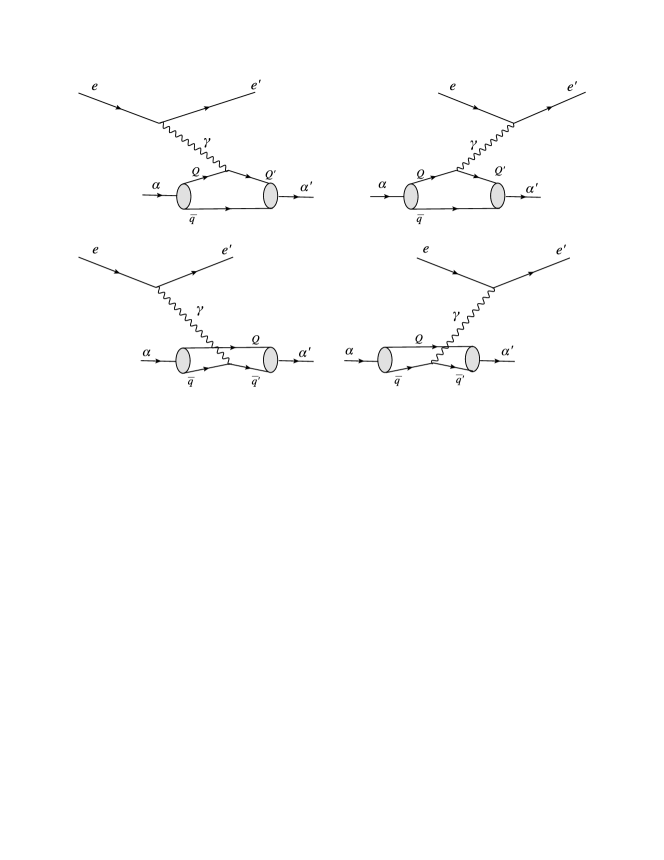
Figure 3.2: The 4 time orderings of photon exchange contributing to the optical potential (3.1). The two graphs in the first row contribute to $J^{\nu}_{Q}$, the other two graphs to $J^{\nu}_{\bar{q}}$.

3.2 Weak decays

We will use the same procedure to extract weak meson transition currents from the invariant amplitudes for semileptonic meson decays. We will illustrate it for the particular case of the $\bar{B}^{0}\to D^{(*)+}e\bar{\nu}_{e}$ decay. The coupled-channel mass operator differs from the electromagnetic case in the number of particles in the initial, final as well as intermediate states. The matrix mass operator to be considered requires at least four channels

$$\left(\begin{array}[]{cccc}\hat{M}^{\mathrm{conf}}_{b\bar{d}}&0&\hat{K}_{c\bar{d}W\rightarrow b\bar{d}}&\hat{K}_{b\bar{d}We\bar{\nu}_{e}\rightarrow b\bar{d}}\\ 0&\hat{M}^{\mathrm{conf}}_{c\bar{d}e\bar{\nu}_{e}}&\hat{K}_{c\bar{d}W\rightarrow c\bar{d}e\bar{\nu}_{e}}&\hat{K}_{b\bar{d}We\bar{\nu}_{e}\rightarrow c\bar{d}e\bar{\nu}_{e}}\\ \hat{K}^{\dagger}_{c\bar{d}W\rightarrow b\bar{d}}&\hat{K}^{\dagger}_{c\bar{d}W\rightarrow c\bar{d}e\bar{\nu}_{e}}&\hat{M}^{\mathrm{conf}}_{c\bar{d}W}&0\\ \hat{K}^{\dagger}_{b\bar{d}We\bar{\nu}_{e}\rightarrow b\bar{d}}&\hat{K}^{\dagger}_{b\bar{d}We\bar{\nu}_{e}\rightarrow c\bar{d}e\bar{\nu}_{e}}&0&\hat{M}^{\mathrm{conf}}_{b\bar{d}We\bar{\nu}_{e}}\end{array}\right)\,.$$ (3.17)

Applying a Feshbach reduction to eliminate the $W$-boson channels one obtains the transition potential

$$\hat{V}_{\mathrm{opt}}^{b\bar{d}\rightarrow c\bar{d}e\bar{\nu}_{e}}(m)=\hat{K}_{c\bar{d}W\rightarrow c\bar{d}e\bar{\nu}_{e}}(m-M^{\mathrm{conf}}_{c\bar{d}W})^{-1}\hat{K}^{\dagger}_{c\bar{d}W\rightarrow b\bar{d}}$$ (3.18)

$$+\hat{K}_{b\bar{d}We\bar{\nu}_{e}\rightarrow c\bar{d}e\bar{\nu}_{e}}(m-\hat{M}^{\mathrm{conf}}_{b\bar{d}We\bar{\nu}_{e}})^{-1}\hat{K}^{\dagger}_{b\bar{d}We\bar{\nu}_{e}\rightarrow b\bar{d}}\,.$$

Each term accounts for one time-ordered contribution of the $W$ exchange. The process is sketched in Fig. 3.3.

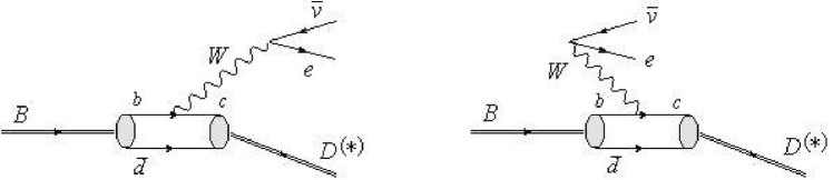
Figure 3.3: The two time-ordered contributions to the semileptonic weak decay of a $\bar{B}^{0}$ into a $D^{(\ast)+}$ meson.

Denoting again the discrete quantum numbers of the confined systems $B$ and $D^{(*)}$ by $\alpha$ and $\alpha^{\prime}$ the invariant decay amplitude becomes

$$\langle\underline{v}^{\prime};\vec{\underline{k}}_{e}^{\prime},\underline{\mu}_{e}^{\prime};\vec{\underline{k}}_{\bar{\nu}_{e}}^{\prime};\vec{\underline{k}}_{\alpha^{\prime}}^{\prime},\underline{\mu}_{\alpha^{\prime}}^{\prime},\alpha^{\prime}|\hat{V}_{\mathrm{opt}}^{b\bar{d}\rightarrow c\bar{d}e\bar{\nu}_{e}}(m)|\vec{\underline{k}}_{\alpha},\underline{\mu}_{\alpha},\alpha\rangle_{\mathrm{os}}\,$$

$$=\langle\underline{v}^{\prime};\vec{\underline{k}}_{e}^{\prime},\underline{\mu}_{e}^{\prime};\vec{\underline{k}}_{\bar{\nu}_{e}}^{\prime};\vec{\underline{k}}_{\alpha^{\prime}}^{\prime},\underline{\mu}_{\alpha^{\prime}}^{\prime},\alpha^{\prime}|\mathds{1}_{e\bar{\nu}_{e}c\bar{d}}\hat{K}_{c\bar{d}W\rightarrow c\bar{d}e\bar{\nu}_{e}}(m-M^{\mathrm{conf}}_{c\bar{d}W})^{-1}\mathds{1}_{Wc\bar{d}}\hat{K}^{\dagger}_{c\bar{d}W\rightarrow b\bar{d}}\mathds{1}_{b\bar{d}}$$

$$+\hat{K}_{b\bar{d}We\bar{\nu}_{e}\rightarrow c\bar{d}e\bar{\nu}_{e}}(m-\hat{M}^{\mathrm{conf}}_{b\bar{d}We\bar{\nu}_{e}})^{-1}\mathds{1}_{b\bar{d}W\bar{\nu}_{e}}\hat{K}^{\dagger}_{b\bar{d}We\bar{\nu}_{e}\rightarrow b\bar{d}}\mathds{1}_{b\bar{d}}|\vec{\underline{k}}_{\alpha},\underline{\mu}_{\alpha},\alpha\rangle_{\mathrm{os}}\,,$$

where “on-shell” (“os”) means $m=m_{B}=\omega_{\underline{k}_{\alpha}}=\omega_{\underline{k}^{\prime}_{\alpha}}+\omega_{\underline{k}^{\prime}_{e}}+\omega_{\underline{k}^{\prime}_{\bar{\nu}_{e}}}$. It is necessary again to introduce completeness relations between the operators that form the optical potential in order to calculate the matrix elements in Eq. (3.2). Thereby we obtain again the corresponding expressions for the wave functions and matrix elements of the interaction vertices. In the case of weak decays the latter are determined by the weak interaction density $\mathcal{L}^{\text{wk}}_{\text{int}}(x)$.

Proceeding in the same way in the calculation of matrix elements and wave functions as in the electromagnetic case (explicit expressions are given in App. B) one obtains for the on-shell matrix elements of $\hat{V}_{\mathrm{opt}}^{b\bar{d}\rightarrow c\bar{d}e\bar{\nu}_{e}}(m)$ the same structure as for the invariant $B\to D^{(*)}e\bar{\nu}_{e}$ decay amplitude that results from leading-order covariant perturbation theory:

$$\langle\underline{v}^{\prime};\vec{\underline{k}}_{e}^{\prime},\underline{\mu}_{e}^{\prime};\vec{\underline{k}}_{\bar{\nu}_{e}}^{\prime};\vec{\underline{k}}_{\alpha^{\prime}}^{\prime},\underline{\mu}_{\alpha^{\prime}}^{\prime},\alpha^{\prime}|\hat{V}_{\mathrm{opt}}^{b\bar{d}\rightarrow c\bar{d}e\bar{\nu}_{e}}(m)|\vec{\underline{k}}_{\alpha},\underline{\mu}_{\alpha},\alpha\rangle_{\mathrm{os}}$$ (3.20)

$$= \underline{v}_{0}\delta^{3}(\vec{\underline{v}}^{\,\prime}-\vec{\underline{v}}\,)\,\frac{(2\pi)^{3}}{\sqrt{(\omega_{\underline{k}_{e}^{\prime}}+\omega_{\underline{k}_{\bar{\nu}_{e}}^{\prime}}+\omega_{\underline{k}_{\alpha^{\prime}}^{\prime}})^{3}}\sqrt{\omega_{\underline{k}_{\alpha}^{\phantom{\prime}}}^{3}}}$$

$$\times\frac{e^{2}}{2\sin^{2}\vartheta_{\mathrm{w}}}V_{cb}\,\frac{1}{2}\underbrace{\bar{u}_{\underline{\mu}_{e}^{\prime}}(\vec{\underline{k}}_{e}^{\prime})\gamma^{\mu}(1-\gamma^{5})v_{\underline{\mu}_{\bar{\nu}_{e}}^{\prime}}(\vec{\underline{k}}_{\bar{\nu}_{e}}^{\prime})}_{j_{\bar{\nu}_{e}\rightarrow e}^{\mu}(\vec{\underline{k}}_{e}^{\prime},\underline{\mu}_{e}^{\prime};\vec{\underline{k}}_{\bar{\nu}_{e}}^{\prime},\underline{\mu}_{\bar{\nu}_{e}}^{\prime})}$$

$$\times\frac{(-g_{\mu\nu})}{(\underline{k}^{\prime}_{e}+\underline{k}^{\prime}_{\bar{\nu}_{e}})^{2}-m_{W}^{2}}\frac{1}{2}{J_{\alpha\rightarrow\alpha^{\prime}}^{\nu}(\vec{\underline{k}}_{\alpha^{\prime}}^{\prime},\underline{\mu}_{\alpha^{\prime}}^{\prime};\vec{\underline{k}}_{\alpha},\underline{\mu}_{\alpha})}\,.$$

Here $\vartheta_{\mathrm{w}}$ denotes the electroweak mixing angle and $e$ the usual elementary electric charge and $V_{cb}$ is the Cabibbo-Kobayashi-Maskawa matrix element occurring at the $Wbc$-vertex.

Pseudoscalar-to-pseudoscalar transitions

If $\alpha$ and $\alpha^{\prime}$ are the quantum numbers of $B$ and $D$ mesons, respectively, the weak transition current turns out to have the form

$$J^{\nu}_{B\rightarrow D}(\vec{\underline{k}}_{D}^{\prime};\vec{\underline{k}}_{B}=\vec{0}) = \frac{\sqrt{\omega_{\underline{k}_{B}}\omega_{\underline{k}_{D}^{\prime}}}}{4\pi}\int\,\frac{d^{3}\tilde{k}_{\bar{q}}^{\prime}}{2\omega_{k_{b}}}\,\sqrt{\frac{\omega_{\tilde{k}^{\prime}_{c}}+\omega_{\tilde{k}^{\prime}_{\bar{q}}}}{\omega_{{k}^{\prime}_{c}}+\omega_{{k}^{\prime}_{\bar{q}}}}}\,\sqrt{\frac{\omega_{\tilde{k}_{b}}\omega_{\tilde{k}_{\bar{q}}}}{\omega_{\tilde{k}^{\prime}_{c}}\omega_{\tilde{k}^{\prime}_{\bar{q}}}}}\,$$ (3.21)

$$\times\bigg{\{}\!\sum_{\mu_{b},\mu_{c}^{\prime}=\pm\frac{1}{2}}\!\!\!\bar{u}_{\mu_{c}^{\prime}}(\vec{k}_{c}^{\prime})\,\gamma^{\nu}\,(1-\gamma^{5})\,u_{\mu_{b}}(\vec{k}_{b})$$

$$\times D^{1/2}_{\mu_{b}\mu_{c}^{\prime}}\!\left[\!R_{\mathrm{W}}\!\left(\frac{\tilde{k}_{\bar{q}}^{\prime}}{m_{\bar{q}}},B_{c}(v_{c\bar{q}}^{\prime})\right)\,\!R^{-1}_{\mathrm{W}}\!\left(\frac{\tilde{k}_{c}^{\prime}}{m_{c}},B_{c}(v_{c\bar{q}}^{\prime})\right)\right]\bigg{\}}\,$$

$$\times\psi^{\ast}_{D}\,(|\vec{\tilde{k}}_{\bar{q}}^{\prime}|)\,\psi_{B}\,(|\vec{\tilde{k}}_{\bar{q}}|)\,.$$

The structure of the current is, of course, very similar to the electromagnetic case. Here the point-like current is the one that comes from the $Wbc$-vertex. $\psi_{B}$ as well as $\psi_{D}$ (and in the following $\psi_{D^{\ast}}$) are normalized like in Eq. (3.15). The expression is simpler than in the electromagnetic case, since the initial state is at rest and therefore $\vec{\tilde{k}}_{\bar{q}}=\vec{k}_{\bar{q}}=-\vec{k}_{b}=-\vec{\tilde{k}}_{b}$. There are no relativistic spin-rotation effects on the initial state and the Wigner $D$-functions refer only to the final $c\bar{q}$ state.

Pseudoscalar-to-vector transitions

In the transition where the spin of the meson also changes, i.e. $B\to D^{*}e\bar{\nu}_{e}$, one has to take into account the corresponding Clebsch-Gordan coefficients that couple the quarks to the spin-1 $D^{*}$ meson. This affects the current such that it differs from the previous one in the way how the Wigner rotations act on the spin components. In this case there are independent rotations that act on each of the constituents:

$$J^{\nu}_{B\rightarrow D^{\ast}}(\vec{\underline{k}}_{D^{\ast}}^{\prime},\underline{\mu}_{D^{\ast}}^{\prime};\vec{\underline{k}}_{B}=\vec{0})=\!\!\frac{\sqrt{\omega_{\underline{k}_{B}}\omega_{\underline{k}_{D^{\ast}}^{\prime}}}}{4\pi}\int\,\frac{d^{3}\tilde{k}_{\bar{q}}^{\prime}}{2\omega_{k_{b}}}\,\sqrt{\frac{\omega_{\tilde{k}^{\prime}_{c}}+\omega_{\tilde{k}^{\prime}_{\bar{q}}}}{\omega_{{k}^{\prime}_{c}}+\omega_{{k}^{\prime}_{\bar{q}}}}}\,\sqrt{\frac{\omega_{\tilde{k}_{b}}\omega_{\tilde{k}_{\bar{q}}}}{\omega_{\tilde{k}^{\prime}_{c}}\omega_{\tilde{k}^{\prime}_{\bar{q}}}}}\,$$

$$\quad\times\bigg{\{}\!\sum_{\mu_{b},\mu_{c}^{\prime},\tilde{\mu}_{c}^{\prime},\tilde{\mu}_{\bar{q}}^{\prime}=\pm\frac{1}{2}}\!\!\!\!\!\!\bar{u}_{\mu_{c}^{\prime}}(\vec{k}_{c}^{\prime})\,\gamma^{\nu}\,(1-\gamma^{5})u_{\mu_{b}}(\vec{k}_{b})$$

$$\quad\quad\quad\quad\quad\quad\times\sqrt{2}(-1)^{\frac{1}{2}-\mu_{b}}C^{1\mu^{\prime}_{\!D^{\ast}}}_{\frac{1}{2}\tilde{\mu}_{c}^{\prime}\frac{1}{2}\tilde{\mu}_{\bar{q}}^{\prime}}\,D^{1/2}_{\tilde{\mu}_{c}^{\prime}\mu_{c}^{\prime}}\!\left[\!R^{-1}_{\mathrm{W}}\!\left(\frac{\tilde{k}_{c}^{\prime}}{m_{c}},B_{c}(v_{c\bar{q}}^{\prime})\right)\right]\,$$

$$\quad\quad\quad\quad\quad\quad\times D^{1/2}_{\tilde{\mu}_{\bar{q}}^{\prime}-\mu_{b}}\!\left[\!R^{-1}_{\mathrm{W}}\!\left(\frac{\tilde{k}^{\prime}_{\bar{q}}}{m_{\bar{q}}},B^{-1}_{c}(v_{c\bar{q}}^{\prime})\right)\right]\bigg{\}}\,\psi^{\ast}_{D^{\ast}}\,(|\vec{\tilde{k}}_{\bar{q}}^{\prime}|)\,\psi_{B}\,(|\vec{\tilde{k}}_{\bar{q}}|)\,.$$

3.3 Dynamical exchange potential

We have seen that the number of channels to be considered depends on the kind of process one is interested in. Up till now we have only considered the electroweak structure of $q\bar{q}$-bound states that were generated by instantaneous confining forces. In the following we will also be interested in the electroweak structure of bound states that are caused by dynamical particle exchange. Treating explicitly the dynamics of the exchange particles that are responsible for the binding requires the introduction of additional channels in the mass operator. In Chap. 8 we will investigate the electromagnetic structure of the deuteron, considered as a neutron-proton bound state caused by dynamical $\sigma$-meson exchange. The general mass eigenvalue problem for electron-deuteron scattering in this case then needs 4-channels,

$$\left(\begin{array}[]{cccc}\hat{M}_{enp}&\hat{K}_{\gamma}&\hat{K}_{\sigma}&0\\ \hat{K}_{\gamma}^{\dagger}&\hat{M}_{enp\gamma}&0&\hat{K}_{\sigma}\\ \hat{K}_{\sigma}^{\dagger}&0&\hat{M}_{enp\sigma}&\hat{K}_{\gamma}\\ 0&\hat{K}_{\sigma}^{\dagger}&\hat{K}_{\gamma}^{\dagger}&\hat{M}_{enp\gamma\sigma}\end{array}\right)\left(\begin{array}[]{c}|\psi_{enp}\rangle\\ |\psi_{enp\gamma}\rangle\\ |\psi_{enp\sigma}\rangle\\ |\psi_{enp\gamma\sigma}\rangle\end{array}\right)=m\left(\begin{array}[]{c}|\psi_{enp}\rangle\\ |\psi_{enp\gamma}\rangle\\ |\psi_{enp\sigma}\rangle\\ |\psi_{enp\gamma\sigma}\rangle\end{array}\right).$$ (3.23)

Additional relativistic effects become important when the retardation of the meson exchange that binds the nucleons is comparable to the one of the photon exchange. This leads to, so-called, exchange currents.

Chapter 4 Currents and form factors

We will dedicate this chapter to the study of the properties of the current derived by means of the method explained above. The current is extracted in each case from the invariant one-boson-exchange amplitude for electron-meson scattering and weak semileptonic decays. No particular ansatz is made for the current that imposes the desired properties that such a current should have. It is therefore necessary to examine the properties of our currents, in order to check that the procedure carried out makes sense. The essential properties that the current should fulfill are: Lorentz covariance, i.e. the current must transform like a 4-vector under Lorentz transformations; current conservation for electromagnetic scattering, i.e. $\partial_{\mu}\tilde{J}^{\mu}_{[\alpha]}=0$; and cluster separability or macrocausality. Cluster separability means in this context that the hadron currents and the corresponding form factors should depend on the hadron properties only, and not on the ones of the particle with which it interacts. Once one is able to understand the properties of the hadron currents, it will be possible to provide consistent analytical expressions for the form factors, as deduced from them.

4.1 Electromagnetic form factors

4.1.1 Pseudoscalar bound states

Covariance and current conservation

We first check whether the current transforms like a 4-vector under Lorentz transformations. If one looks at the current (3.14) and applies a Lorentz transformation $\Lambda$ it turns out that $\tilde{J}^{\nu}_{[\alpha]}(\underline{\vec{k}}^{\prime}_{\alpha};\underline{\vec{k}}_{\alpha})$ does not transform like a 4-vector. Instead, the current transforms by the Wigner rotation $R_{W}(v,\Lambda)$, where $v$ is the overall 4-velocity of the electron-meson system [20]. This is due to the fact that $\tilde{J}^{\nu}_{[\alpha]}(\underline{\vec{k}}^{\prime}_{\alpha};\underline{\vec{k}}_{\alpha})$ is computed using velocity states, which do not transform like 4-vectors under Lorentz transformations, they transform by a Wigner rotation instead (cf. Sec. 2.3.2). Going back to the physical meson momenta $\underline{p}_{\alpha}^{(^{\prime})}=B_{c}(v)\underline{k}_{\alpha}^{(^{\prime})}$, which do transform like 4-vectors, one finds that the current has the desired transformation properties:

$$\tilde{J}_{[\alpha]}^{\nu}(\vec{\underline{p}}_{\alpha}^{\prime};\vec{\underline{p}}_{\alpha}):=[B_{c}(\underline{v})]^{\nu}_{\phantom{\nu}\rho}\tilde{J}_{[\alpha]}^{\rho}(\vec{\underline{k}}_{\alpha}^{\prime};\vec{\underline{k}}_{\alpha})\,.$$ (4.1)

$\tilde{J}_{[\alpha]}^{\nu}(\vec{\underline{p}}_{\alpha}^{\prime};\vec{\underline{p}}_{\alpha})$ transforms like a 4-vector and is a conserved current, i.e. $(\underline{p}_{\alpha}-\underline{p}_{\alpha}^{\prime})_{\nu}\tilde{J}_{[\alpha]}^{\nu}(\vec{\underline{p}}_{\alpha}^{\prime};\vec{\underline{p}}_{\alpha})=0$. A more detailed discussion of transformation properties and current conservation can be found in Refs. [20, 21].

Cluster separability

The next task is to investigate if the current satisfies the desired cluster separability properties. For a pseudoscalar meson, one expects a current of the form

$$J_{[\alpha]}^{\nu}(\vec{\underline{p}}_{\alpha}^{\prime};\vec{\underline{p}}_{\alpha})=(\underline{p}_{\alpha}+\underline{p}^{\prime}_{\alpha})^{\nu}\,F(\text{Q}^{2}).$$ (4.2)

It is known, however, that the Bakamjian-Thomas construction leads to problems with cluster separability. Basis states which are appropriate to represent Bakamjian-Thomas type mass operators (like our velocity states) use variables to represent relative momenta which do not have a physical interpretation in the presence of interactions [4]. As a consequence, problems with macroscopic locality appear. A manifestation of such problems is that our microscopic current contains non-physical contributions. It cannot be expressed in terms of hadronic covariants only, but one needs an additional covariant associated with the electron four-momenta [14, 21]:

$$\tilde{J}_{[\alpha]}^{\nu}(\vec{\underline{p}}_{\alpha}^{\prime};\vec{\underline{p}}_{\alpha})=(\underline{p}_{\alpha}+\underline{p}^{\prime}_{\alpha})^{\nu}\,f(\text{Q}^{2},s)+(\underline{p}_{e}+\underline{p}^{\prime}_{e})^{\nu}\,g(\text{Q}^{2},s)\,.$$ (4.3)

The impossibility of decomposing the current as in Eq. (4.2) shows up when one tries to extract the form factor from the different non-vanishing components of the current, since it turns out that this cannot be done unambiguously. Furthermore, the form factors associated with the covariants depend not only on the 4-momentum transfer squared (Mandelstam $t$), but also on the Mandelstam $s=(\underline{p}_{e}+\underline{p}_{\alpha})^{2}$, i.e. the square of the invariant mass of the electron-meson system.

The necessity of non-physical covariants and corresponding form factors resembles the occurrence of analogous contributions within the covariant light-front formulation of Carbonell et al. [22]. In the covariant light-front approach the unphysical covariants contain a 4-vector $\omega^{\mu}$, which specifies the orientation of the light front and which has to be introduced to render the front-form approach manifestly covariant. In the present case, the problem is related to cluster separability violation caused by the Bakamjian-Thomas construction.

For a better understanding of these unphysical features we have undertaken a numerical study. Since the form factors are functions of Lorentz invariants we are free to choose the frame in which they are extracted. Without loss of generality we choose a center-of-momentum frame in which $\vec{v}=\vec{0}$, i.e. $\underline{\vec{p}}^{(\prime)}_{\alpha}=\underline{\vec{k}}^{(\prime)}_{\alpha}$, and

$$\underline{\vec{k}}_{\alpha}=-\underline{\vec{k}}_{e}=\left(\begin{array}[]{c}-\frac{\text{Q}}{2}\\ 0\\ \sqrt{\kappa_{\alpha}^{2}-\frac{\text{Q}^{2}}{4}}\end{array}\right)\,\quad\hbox{and}\quad\vec{q}=\left(\begin{array}[]{c}-\text{Q}\\ 0\\ 0\end{array}\right)\,,$$ (4.4)

where $\kappa_{\alpha}:=|\underline{\vec{k}}_{\alpha}|=|\underline{\vec{k}}_{\alpha}^{\prime}|$. In this parametrization the modulus of the relative momentum is subject to the constraint that $\kappa_{\alpha}^{2}\geq\text{Q}^{2}/4$, which means that $s\geq m_{\alpha}^{2}+m_{e}^{2}+\text{Q}^{2}/2+2\sqrt{m_{\alpha}^{2}+\text{Q}^{2}/4}\sqrt{m_{e}^{2}+\text{Q}^{2}/4}$.

The only non-vanishing components of the current within this kinematics are $\tilde{J}_{[\alpha]}^{0}$ and $\tilde{J}_{[\alpha]}^{3}$ from which the form factors $f(\text{Q}^{2},s)$ and $g(\text{Q}^{2},s)$ can be extracted by inserting the microscopic expression (cf. Eqs. (3.1) and (3.14)) for $\tilde{J}_{[\alpha]}^{\nu}$ on the left-hand side of Eq. (4.3):

$$f(\text{Q}^{2},s)=\frac{1}{\left(1+\frac{\sqrt{\kappa_{\alpha}^{2}+m_{\alpha}^{2}}}{\sqrt{\kappa_{\alpha}^{2}+m_{e}^{2}}}\right)}\left(\frac{\tilde{J}^{0}_{[\alpha]}(\underline{p}_{\alpha},\underline{p}_{\alpha}^{\prime})}{2\sqrt{\kappa_{\alpha}^{2}+m_{e}^{2}}}+\frac{\tilde{J}^{3}_{[\alpha]}(\underline{p}_{\alpha},\underline{p}_{\alpha}^{\prime})}{2\sqrt{\kappa_{\alpha}^{2}-\frac{\text{Q}^{2}}{4}}}\right),$$ (4.5)

$$g(\text{Q}^{2},s)=\frac{1}{\left(1+\frac{\sqrt{\kappa_{\alpha}^{2}+m_{e}^{2}}}{\sqrt{\kappa_{\alpha}^{2}+m_{\alpha}^{2}}}\right)}\left(\frac{\tilde{J}^{0}_{[\alpha]}(\underline{p}_{\alpha},\underline{p}_{\alpha}^{\prime})}{2\sqrt{\kappa_{\alpha}^{2}+m_{\alpha}^{2}}}-\frac{\tilde{J}^{3}_{[\alpha]}(\underline{p}_{\alpha},\underline{p}_{\alpha}^{\prime})}{2\sqrt{\kappa_{\alpha}^{2}-\frac{\text{Q}^{2}}{4}}}\right).$$ (4.6)

For the bound state wave function, we use the simple harmonic-oscillator form (6.1). For further comparison we take the oscillator parameter as well as the constituent-quark masses to be the same as in Ref. [34] (see also Table 6.1), where form factors of heavy-light mesons were calculated within the front-form approach. The dependence of these form factors on Mandelstam-$s$ is plotted for the $D^{+}$ and $B^{-}$ mesons in Figs. 4.1 and 4.2 for different values of the momentum transfer $\text{Q}^{2}$. For $s\to\infty$ the spurious form factor vanishes and the $s$-dependence of the physical form factor disappears with increasing $s$. It is therefore suggestive to take the $s\to\infty$ limit to get rid of cluster-separability violating effects and obtain sensible results for the physical form factors. Taking $s\to\infty$ can be understood as extracting the form factor in the infinite-momentum frame of the meson. It is equivalent to taking $\kappa_{\alpha}\to\infty$.

Similar calculations were done for mesons of equal constituent masses [20, 21]. For light-light systems the resulting analytical expression for the electromagnetic form factor of a pseudoscalar meson were proved to be equivalent to the usual front-form result, obtained for a one-body current in the $q^{+}=0$ frame [20]. For heavy-light systems the situation becomes more intricate. One can observe that the rate of convergence to the $s\to\infty$ limit decreases with increasing the heavy-quark mass. In order to extract the Isgur-Wise function one has to be cautious when taking the heavy-quark limit $m_{Q}\to\infty$. This matter will be discussed in detail in the next chapter.

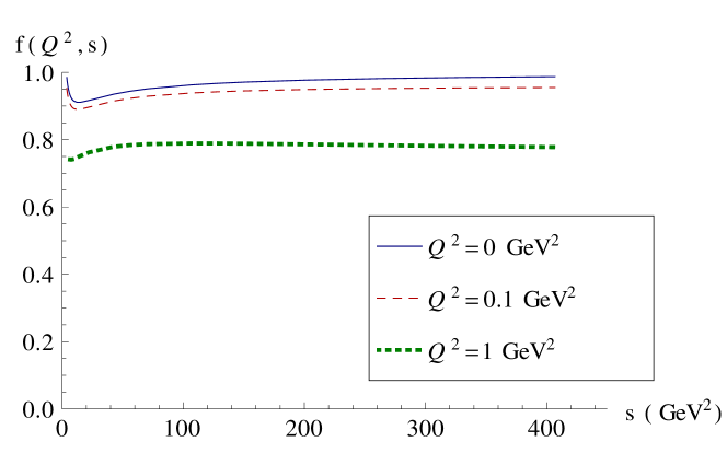
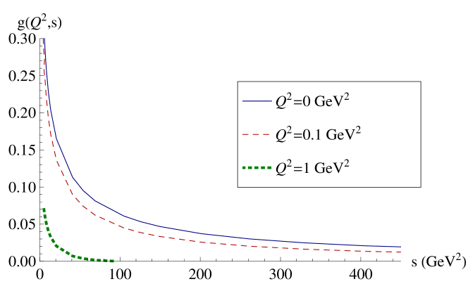
Figure 4.1: Mandelstam-$s$ dependence of the physical and spurious $D^{+}$ electromagnetic form factors $f(\text{Q}^{2},s)$ and $g(\text{Q}^{2},s)$, respectively, for different values of $\text{Q}^{2}$ ($0$ GeV² solid, $0.1$ GeV² dashed, $1$ GeV² dotted) calculated with the oscillator wave function (6.1), and (mass) parameters given in Table 6.1.

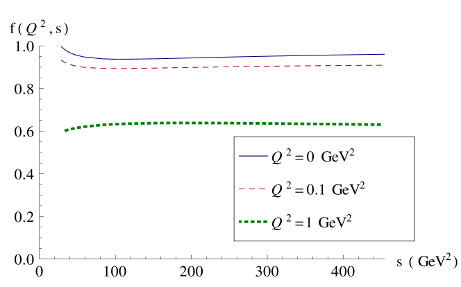
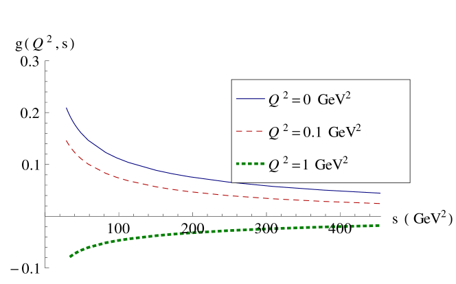
Figure 4.2: Mandelstam-$s$ dependence of the physical and spurious $B^{-}$ electromagnetic form factors $f(\text{Q}^{2},s)$ and $g(\text{Q}^{2},s)$, respectively, for different values of $\text{Q}^{2}$ ($0$ GeV² solid, $0.1$ GeV² dashed, $1$ GeV² dotted) calculated with the oscillator wave function (6.1), and (mass) parameters given in Table 6.1.

4.1.2 Vector bound states

Hermiticity, covariance, current conservation, the angular condition and other properties like cluster separability, were analyzed in detail in Ref. [21] for spin-1 bound-state currents of two-body systems with equal constituent masses within the point-form approach. We summarize in this section the most important points, since they will be necessary to understand further calculations for spin-1 bound states. In Chap. 8 we will use some elements presented here for the study of electromagnetic properties of spin-1 bound states that arise from dynamical particle-exchange forces.

Cluster separability

The covariant decomposition of our electromagnetic current becomes more complicated if one deals with spin-1 bound states. It requires to consider all possible covariants including those that depend on the electron momenta. These are in total 11 covariants, with their associated form factors. The form factors exhibit also a spurious dependence on Mandelstam-$s$. The most general covariant decomposition of the current is given by:

$$\tilde{J}^{\mu}_{[\alpha]}(\underline{\vec{k}}_{\alpha},\underline{\mu}_{\alpha};\underline{\vec{k}}^{\prime}_{\alpha},\underline{\mu}^{\prime}_{\alpha};\underline{K}_{e})=$$

$$\;\;\;=\left[f_{1}(\text{Q}^{2},s)(\epsilon^{\prime*}\cdot\epsilon)+f_{2}(\text{Q}^{2},s)\frac{(\epsilon^{\prime*}\cdot q)(\epsilon^{*}\cdot q)}{2m_{\alpha}^{2}}\right]\underline{K}_{\alpha}^{\mu}$$

$$\;\;\;+g_{M}(\text{Q}^{2},s)\left[\epsilon^{\prime*\mu}(\epsilon\cdot q)-\epsilon^{\mu}(\epsilon^{\prime*}\cdot q)\right]$$

$$\;\;\;+\frac{m^{2}_{\alpha}}{2\underline{K}_{e}\cdot\underline{k}_{\alpha}}\Big{[}b_{1}(\text{Q}^{2},s)(\epsilon^{\prime*}\cdot\epsilon)+b_{2}(\text{Q}^{2},s)\frac{(q\cdot\epsilon^{\prime*})(q\cdot\epsilon^{*})}{m_{\alpha}^{2}}$$

$$\;\;\;\qquad\qquad\qquad+b_{3}(\text{Q}^{2},s)m^{2}_{\alpha}\frac{(\underline{K}_{e}\cdot\epsilon^{\prime*})(\underline{K}_{e}\cdot\epsilon^{*})}{(\underline{K}_{e}\cdot\underline{k}_{\alpha})^{2}}$$

$$\;\;\;\qquad\qquad\qquad+b_{4}(\text{Q}^{2},s)\frac{(q\cdot\epsilon^{\prime*})(\underline{K}_{e}\cdot\epsilon)-(q\cdot\epsilon)(\underline{K}_{e}\cdot\epsilon^{\prime*})}{2(\underline{K}_{e}\cdot\underline{k}_{\alpha})}\Big{]}\underline{K}_{e}^{\mu}$$

$$\;\;\;+\Big{[}b_{5}(\text{Q}^{2},s)m^{2}_{\alpha}\frac{(\underline{K}_{e}\cdot\epsilon^{\prime*})(\underline{K}_{e}\cdot\epsilon)}{(\underline{K}_{e}\cdot\underline{k}_{\alpha})^{2}}$$

$$\;\;\;\qquad+b_{6}(\text{Q}^{2},s)\frac{(q\cdot\epsilon^{\prime*})(\underline{K}_{e}\cdot\epsilon)-(q\cdot\epsilon)(\underline{K}_{e}\cdot\epsilon^{\prime*})}{2\underline{K}_{e}\cdot\underline{k}_{\alpha}}\Big{]}\underline{K}_{\alpha}^{\mu}$$

$$\;\;\;+b_{7}(\text{Q}^{2},s)m^{2}_{\alpha}\frac{\epsilon^{\prime*\mu}(\epsilon\cdot\underline{K}_{e})+\epsilon^{\mu}(\epsilon^{\prime*}\cdot\underline{K}_{e})}{\underline{K}_{e}\cdot\underline{k}_{\alpha}}$$

$$\;\;\;+b_{8}(\text{Q}^{2},s)q^{\mu}\frac{(q\cdot\epsilon^{\prime*})(\underline{K}_{e}\cdot\epsilon)+(q\cdot\epsilon)(\underline{K}_{e}\cdot\epsilon^{\prime*})}{2\underline{K}_{e}\cdot\underline{k}_{\alpha}}.$$

(4.7)

where the shorthand notations $\underline{K}_{e(\alpha)}:=\underline{k}_{e(\alpha)}+\underline{k}_{e(\alpha)}^{\prime}$ and $\epsilon^{(\prime)}:=\epsilon(\underline{\vec{k}}_{\alpha}^{(\prime)},\underline{\mu}_{\alpha}^{(\prime)})$, have been used, the latter being the polarization vectors of the incoming and outgoing spin-1 bound state (cf. App. A.1.2). Only 3 of the 11 form factors have a physical meaning, namely $f_{1}$, $f_{2}$ and $g_{M}$. For a detailed discussion about the elimination of these spurious contributions in the infinite-momentum frame the reader may consult Ref. [21]. The numerical analysis carried out in Ref. [21] (that uses the kinematics we have considered in Eq. (4.4)) reveals that 4 of the 8 spurious contributions cannot be eliminated by simply taking $s\to\infty$ as in the pseudoscalar case. The form factors $b_{5}$, $b_{6}$, $b_{7}$ and $b_{8}$ do not vanish in the infinite-momentum frame. These spurious contributions in the current are relatively small, but may have important consequences on some properties of the current if they are not treated properly.

Covariance, current conservation and angular condition

As in the pseudoscalar case, our microscopic expression for the electromagnetic current of a spin-1 bound state transforms like a 4-vector under Lorentz transformations if one goes back to the physical meson momenta by applying a canonical boost $\underline{p}^{(\prime)}_{\alpha}=B_{c}(v)\underline{k}^{(\prime)}_{\alpha}$ [21].

Because of the non-vanishing $b_{7}$ and $b_{8}$, the current (4.1.2) is not conserved; and the $b_{5}$ and $b_{7}$ violate the so-called angular condition. Let us abbreviate the notation by calling $B_{i}(\text{Q}^{2}):=\lim_{s\to\infty}b_{i}(\text{Q}^{2},s)$ and $J^{\mu}_{\underline{\mu}_{\alpha}^{\prime}\underline{\mu}_{\alpha}}:=\tilde{J}^{\mu}_{[\alpha]}(\underline{\vec{k}}_{\alpha},\underline{\mu}_{\alpha};\underline{\vec{k}}^{\prime}_{\alpha},\underline{\mu}^{\prime}_{\alpha};\underline{K}_{e})$. Without spurious contributions the physical current matrix elements should satisfy the angular condition:

$$(1+2\eta)J^{0}_{11}+J^{0}_{1-1}-2\sqrt{2\eta}J^{0}_{10}-J^{0}_{00}=0,$$ (4.8)

with $\eta=\frac{\text{Q}^{2}}{4m^{2}_{\alpha}}$. The studies carried out in [21] show that, due to the spurious contributions, one gets:

$$(1+2\eta)\tilde{J}^{0}_{11}+\tilde{J}^{0}_{1-1}-2\sqrt{2\eta}\tilde{J}^{0}_{10}-\tilde{J}^{0}_{00}=-|e|\left(B_{5}(\text{Q}^{2})-B_{7}(\text{Q}^{2})\right).$$ (4.9)

Nevertheless, it can be shown (for our kinematics) that there are 3 current matrix elements which do no contain any spurious contributions in the limit $s\to\infty$. This matrix elements are $J^{0}_{11}$, $J^{0}_{1-1}$ and $J^{2}_{11}$. They can be used to extract the physical form factors without ambiguity [21]:

$$F_{1}(\text{Q}^{2}) := \lim_{s\to\infty}f_{1}(\text{Q}^{2},\kappa_{\alpha})=-\lim_{s\to\infty}\frac{1}{2\kappa_{\alpha}}\left(J^{0}_{11}+J^{0}_{1-1}\right),$$ (4.10)

$$F_{2}(\text{Q}^{2}) := \lim_{s\to\infty}f_{2}(\text{Q}^{2},\kappa_{\alpha})=-\frac{1}{\eta}\lim_{s\to\infty}\frac{1}{2\kappa_{\alpha}}J^{0}_{1-1},$$ (4.11)

$$G_{M}(\text{Q}^{2}) := \lim_{s\to\infty}g_{M}(\text{Q}^{2},\kappa_{\alpha})=-\frac{i}{\text{Q}}J^{2}_{11}.$$ (4.12)

4.2 Decay form factors

An analogous study must be done for the weak current obtained from the transition amplitude of radiative decays.

4.2.1 Pseudoscalar-to-pseudoscalar transitions

Covariance

As in the electromagnetic case, the pseudoscalar-to-pseudoscalar transition current turns out to have the right transformation properties under Lorentz transformations after applying the canonical boost $B_{c}(\underline{v})$ that connects the physical momenta with center-of-mass momenta,

$$J^{\nu}_{B\rightarrow D}(\vec{\underline{p}}_{D}^{\prime};\vec{\underline{p}}_{B}):=[B_{c}(\underline{v})]^{\nu}_{\phantom{\nu}\rho}J_{B\rightarrow D}^{\rho}(\vec{\underline{k}}_{D}^{\prime};\vec{\underline{k}}_{B})\,.$$ (4.13)

The way how to extract the form factors of weak transitions is analogous to the electromagnetic case. The covariant decomposition of the weak current for a pseudoscalar-to-pseudoscalar transition reads [50]

$$J^{\nu}_{B\rightarrow D}(\vec{\underline{p}}_{D}^{\prime};\vec{\underline{p}}_{B})=\left((\underline{p}_{B}+\underline{p}_{D}^{\prime})^{\nu}-\frac{m^{2}_{B}-m^{2}_{D}}{\underline{q}^{2}}\,\underline{q}^{\nu}\right)F_{1}(\underline{q}^{2})+\frac{m_{B}^{2}-m_{D}^{2}}{\underline{q}^{2}}\,\underline{q}^{\nu}F_{0}(\underline{q}^{2})\,,$$ (4.14)

with the time-like 4-momentum transfer $\underline{q}=(\underline{p}_{B}-\underline{p}_{D})$.

Cluster separability

When one inserts the current (3.21) into Eq. (4.14), and extracts of the form factors $F_{1}$ and $F_{0}$ it turns out that the solution is unique. The form factors can be determined unambiguously from the components of the current $J^{\nu}_{B\to D}$, without the necessity of introducing additional spurious covariants. The form factors do not depend on any other Lorentz invariant quantity different from the 4-momentum transfer $q^{2}$. Unlike in the electromagnetic case, wrong cluster properties of the Bakamjian-Thomas construction do not show up in the structure of the currents and the dependence of the form factors on the available Lorentz invariants.

Since the decay current (4.13) transforms like a 4-vector we can analyze it, without loss of generality, in the frame in which the decaying $B$-meson is at rest (which corresponds to $\vec{v}=\vec{0}$). We parametrize the meson momenta by:

$$\underline{k}_{B}=\left(\begin{array}[]{c}m_{B}\\ 0\\ 0\\ 0\end{array}\right)\quad\hbox{and}\quad\underline{k}_{D}^{\prime}=\left(\begin{array}[]{c}\sqrt{m_{D}^{2}+\kappa_{D}^{2}}\\ \kappa_{D}\\ 0\\ 0\end{array}\right)$$ (4.15)

with

$$\kappa_{D}^{2}=\frac{1}{4m_{B}^{2}}(m_{B}^{2}+m_{D}^{2}-\underline{q}^{2})^{2}-m_{D}^{2}\,.$$ (4.16)

$\kappa_{D}:=|\underline{\vec{k}}_{D}^{\prime}|$ is constrained by the condition $0\leq\kappa_{D}^{2}\leq(m_{B}^{2}-m_{D}^{2})^{2}/(4m_{B}^{2})$, since

$$0\leq\underline{q}^{2}\leq(m_{B}-m_{D})^{2}\,.$$ (4.17)

In order to understand the observation that the decay current $J^{\nu}_{B\rightarrow D}$ is not spoiled by cluster separability problems whereas the electromagnetic current $\tilde{J}_{[\alpha]}^{\nu}$ was, let us note a few points:

• The spurious contributions to the electromagnetic current had their origin in the fact that the calculation was carried out in the center-of-momentum frame of the electron-meson system. Cluster problems appear when different sets of subsystems cannot be isolated properly. In a decay, there is no additional participant in the initial state of the process which could modify the bound-state wave function. Only the final state (electron-antineutrino-meson) might be affected by wrong cluster problems.

• Like in the electromagnetic case, the current (3.21) has only two non-vanishing components (for our chosen kinematics). But unlike in the electromagnetic case, there are now two covariants and associated form factors in the covariant decomposition (4.14) of the decay current; these are $(\underline{p}_{\alpha}+\underline{p}_{\alpha}^{\prime})$ and $(\underline{p}_{\alpha}-\underline{p}_{\alpha}^{\prime})$. In the case of electromagnetic the latter is forbidden by current conservation.

• Form factors are frame independent quantities, therefore one should be able to express them as functions of Lorentz invariant quantities only. In the electromagnetic case the modulus of the three momentum $|\vec{q}|$ cannot be expressed as a function of the squared 4-momentum only, i.e. Mandelstam $t=q^{2}$, but one needs in addition Mandelstam $s$. The modulus of the 3-momentum transfer in the weak decays is, on the other hand, determined by $q^{2}$ only.

4.2.2 Pseudoscalar-to-vector transitions

Covariance

The current (3.2) transforms also like a 4-vector after applying a canonical boost that connects the physical momenta with the center-of-mass momenta, as it happens in the pseudoscalar case. In this case, however, one needs an additional Wigner $D$-function that is associated with the rotation of the $D^{*}$-meson spin:

$$J^{\nu}_{B\rightarrow D^{\ast}}(\vec{\underline{p}}_{D^{\ast}}^{\prime},\underline{\sigma}^{\prime}_{D^{\ast}};\vec{\underline{p}}_{B}):= [B_{c}(\underline{v})]^{\nu}_{\phantom{\nu}\rho}J_{B\rightarrow D^{\ast}}^{\rho}(\vec{\underline{k}}_{D^{\ast}}^{\prime},\underline{\mu}^{\prime}_{D^{\ast}};\vec{\underline{k}}_{B})$$

$$\times D^{1\ast}_{\underline{\mu}^{\prime}_{D^{\ast}}\underline{\sigma}^{\prime}_{D^{\ast}}}\left[R^{-1}_{\mathrm{W}}\!\left({\underline{k}}_{D^{\ast}}^{\prime}/m_{D^{\ast}},B_{c}(v)\right)\right]\,.$$

The most general covariant decomposition of the current is given by [50]

$$J^{\nu}_{B\rightarrow D^{\ast}}(\vec{\underline{p}}_{D^{\ast}}^{\prime},\underline{\sigma}^{\prime}_{D^{\ast}};\vec{\underline{p}}_{B}) =\frac{2i\epsilon^{\nu\mu\rho\sigma}}{m_{B}+m_{D^{*}}}\,\epsilon^{*}_{\mu}(\vec{\underline{p}}_{D^{\ast}}^{\prime},\underline{\sigma}^{\prime}_{D^{\ast}})\,\underline{p}^{\prime}_{D^{\ast}\rho}\,\underline{p}_{B\sigma}\,V(\underline{q}^{2})$$

$$-(m_{B}+m_{D^{*}})\,\epsilon^{*\nu}(\vec{\underline{p}}_{D^{\ast}}^{\prime},\underline{\sigma}^{\prime}_{D^{\ast}})\,A_{1}(\underline{q}^{2})$$

$$+\frac{\epsilon^{*}(\vec{\underline{p}}_{D^{\ast}}^{\prime},\underline{\sigma}^{\prime}_{D^{\ast}})\cdot\underline{q}}{m_{B}+m_{D^{*}}}\,(\underline{p}_{B}+\underline{p}_{D^{\ast}}^{\prime})^{\nu}\,A_{2}(\underline{q}^{2})$$

$$+2m_{D^{*}}\,\frac{\epsilon^{*}(\vec{\underline{p}}_{D^{\ast}}^{\prime},\underline{\sigma}^{\prime}_{D^{\ast}})\cdot\underline{q}}{\underline{q}^{2}}\,\underline{q}^{\nu}\,A_{3}(\underline{q}^{2})$$

$$-2m_{D^{*}}\,\frac{\epsilon^{*}(\vec{\underline{p}}_{D^{\ast}}^{\prime},\underline{\sigma}^{\prime}_{D^{\ast}})\cdot\underline{q}}{\underline{q}^{2}}\,\underline{q}^{\nu}\,A_{0}(\underline{q}^{2})\,,$$ (4.19)

with $\epsilon^{*}(\vec{\underline{p}}_{D^{\ast}}^{\prime},\underline{\sigma}^{\prime}_{D^{\ast}})$ being the polarization 4-vector of the $D^{\ast}$. It appears boosted according to the kinematics used in Eq. (4.15), i.e. (cf. App. A.1.2)

$$\epsilon(\underline{\vec{k}}^{\prime}_{D^{\ast}},\pm 1) = \frac{1}{\sqrt{2}}(\mp\frac{\kappa_{D^{\ast}}}{m_{D^{\ast}}},\mp\sqrt{1+(\frac{\kappa_{D^{\ast}}}{m_{D^{\ast}}})^{2}},-i,0)\,,$$

$$\epsilon(\underline{\vec{k}}^{\prime}_{D^{\ast}},0) = (0,0,0,1)\,.$$ (4.20)

$A_{3}(\underline{q}^{2})$ is a linear combination of $A_{1}(\underline{q}^{2})$ and $A_{2}(\underline{q}^{2})$, namely $A_{3}(\underline{q}^{2})=\frac{m_{B}+m_{D^{\ast}}}{2m_{D^{\ast}}}\,A_{1}(\underline{q}^{2})-\frac{m_{B}-m_{D^{\ast}}}{2m_{D^{\ast}}}A_{2}(\underline{q}^{2})$.

Cluster separability

For the same reasons as in the pseudoscalar-to-pseudoscalar case, the current does not exhibit cluster problems in the form of unphysical contributions to the covariant decomposition, and the form factors can be extracted unambiguously from the independent components of the current. Let us introduce the shorthand notation

$$J^{\nu}(\underline{\mu}^{\prime}_{D^{\ast}}):=J^{\nu}_{B\rightarrow D^{\ast}}(\vec{\underline{k}}_{D^{\ast}}^{\prime},\underline{\mu}^{\prime}_{D^{\ast}};\vec{\underline{k}}_{B}).$$ (4.21)

The non-vanishing components of the current for the kinematics (4.15) are a total of 10, namely $J^{2}(0)$, $J^{3}(0)$, $J^{\mu}(\pm 1)$, $\mu=0,1,2,3$. Taking into account that $J^{\mu}(1)=-J^{\mu}(-1)$, one is left with only 6 different matrix elements, 4 of them being independent. As one can see, $A_{0}$ and $A_{2}$ enter only $J^{0}(1)$ and $J^{1}(1)$. Thus, the set $J^{2}(0)$, $J^{3}(0)$, $J^{0}(1)$ and $J^{1}(1)$ can be used to extract all the $P\to V$ decay form factors. They can be also obtained by means of appropriate projections:

$$V(\underline{q}^{2}) = \frac{i(m_{B}+m_{D^{\ast}})}{2m_{B}^{2}m_{D^{\ast}}^{2}}\left[\left(\frac{m_{B}^{2}+m_{D^{\ast}}^{2}-\underline{q}^{2}}{2m_{B}m_{D^{\ast}}}\right)^{2}-1\right]^{-1}$$ (4.22)

$$\times\epsilon_{\mu}(\vec{\underline{k}}_{D^{\ast}}^{\prime},\underline{\mu}^{\prime}_{D^{\ast}}=0)\,\underline{k}^{\prime}_{D^{\ast}\rho}\,\underline{k}_{B\sigma}\,$$

$$\times\epsilon_{\nu}^{\phantom{\nu}\mu\rho\sigma}J^{\nu}_{B\rightarrow D^{\ast}}(\vec{\underline{k}}_{D^{\ast}}^{\prime},\underline{\mu}^{\prime}_{D^{\ast}}=0;\vec{\underline{k}}_{B})\,,$$

$$A_{0}(\underline{q}^{2}) = \frac{1}{\sqrt{2}m_{B}m_{D^{\ast}}}\left[\left(\frac{m_{B}^{2}+m_{D^{\ast}}^{2}-\underline{q}^{2}}{2m_{B}m_{D^{\ast}}}\right)^{2}-1\right]^{-1/2}$$ (4.23)

$$\times\underline{q}_{\nu}J^{\nu}_{B\rightarrow D^{\ast}}(\vec{\underline{k}}_{D^{\ast}}^{\prime},\underline{\mu}^{\prime}_{D^{\ast}}=1;\vec{\underline{k}}_{B})\,,$$

$$A_{1}(\underline{q}^{2}) = \frac{1}{m_{B}+m_{D^{\ast}}}\,\epsilon_{\nu}(\vec{\underline{k}}_{D^{\ast}}^{\prime},\underline{\mu}^{\prime}_{D^{\ast}}=0)\,$$ (4.24)

$$\times J^{\nu}_{B\rightarrow D^{\ast}}(\vec{\underline{k}}_{D^{\ast}}^{\prime},\underline{\mu}^{\prime}_{D^{\ast}}=0;\vec{\underline{k}}_{B})\,.$$

and

$$A_{2}(\underline{q}^{2})\! = \!\!\frac{\underline{q}^{2}(m_{B}+m_{D^{\ast}})}{4m_{B}^{2}m_{D^{\ast}}^{2}}\left[\left(\frac{m_{B}^{2}+m_{D^{\ast}}^{2}-\underline{q}^{2}}{2m_{B}m_{D^{\ast}}}\right)^{2}\!\!\!\!-1\right]^{-1}$$

$$\times\Bigg{\{}\frac{\sqrt{2}}{m_{B}}\left[\left(\frac{m_{B}^{2}+m_{D^{\ast}}^{2}-\underline{q}^{2}}{2m_{B}m_{D^{\ast}}}\right)^{2}\!\!\!\!-1\right]^{-1/2}\left((\underline{p}_{B}+\underline{p}_{D^{\ast}}^{\prime})-\frac{m^{2}_{B}-m^{2}_{D^{\ast}}}{\underline{q}^{2}}\,\underline{q}\right)_{\nu}$$

$$\quad\times J_{B\rightarrow D^{\ast}}^{\nu}(\vec{\underline{k}}_{D^{\ast}}^{\prime},\underline{\mu}^{\prime}_{D^{\ast}}=1;\vec{\underline{k}}_{B})$$

$$-\left[1-\frac{m_{B}^{2}-m_{D^{\ast}}^{2}}{\underline{q}^{2}}\right]\epsilon_{\nu}(\vec{\underline{k}}_{D^{\ast}}^{\prime},\underline{\mu}^{\prime}_{D^{\ast}}=0)J^{\nu}_{B\rightarrow D^{\ast}}(\vec{\underline{k}}_{D^{\ast}}^{\prime},\underline{\mu}^{\prime}_{D^{\ast}}=0;\vec{\underline{k}}_{B})\Bigg{\}}\,.$$

Having checked the fundamental properties of the electromagnetic and weak currents and knowing how to extract the corresponding form factors unambiguously, we are now in the position to compute the form factors for many different reactions and compare them with experimental data. For simplicity, we will take the same wave function model, namely the harmonic-oscillator wave function used for the numerical studies shown in Fig. 4.1. The parameters are those given in Table 6.1, which allow also for comparisons with front-form calculations. The discussion of the numerical results will be presented in Chap. 7. The method admits, of course, a much wider range of binding forces, namely all those which are compatible with the Bakamjian-Thomas construction.

Chapter 5 Heavy-quark symmetry

The formalism presented as far provides a way of calculating electroweak form factors of two-body bound states and it is general enough to allow for different masses of the constituents, such that we are able to study heavy-light mesons. A requirement for any approach that attempts to describe this kind of systems is to be able to reflect the heavy-quark symmetry predictions in the limit in which one of the constituent masses goes to infinity. The aim of this chapter is to examine the features of our formalism that emerge in the heavy-quark limit, $m_{Q}\to\infty$ (a precise definition of the limit will be given in the next section). The heavy-quark limit provides additional symmetries beyond QCD [10]. Hadrons containing a single heavy quark share physical properties that make them simpler to describe. These properties are often used to design constituent quark models that describe heavy-light systems. The work presented here, by contrast, starts from the most general case of systems of different constituent masses. It is the aim of this section to study if the requirements of heavy-quark symmetry emerge if the mass of the heavy quark goes to infinity.

When the mass of the heavy particle of a system is heavy enough (in hadrons this means in practice $m_{Q}\gg\Lambda_{QCD}$) the behavior of the light quarks does not depend on the flavor of the heavy quark. Mathematically, what one obtains is that matrix elements do not depend on the heavy quark mass – flavor symmetry – or on the heavy quark spin – spin symmetry. The heavy-quark limit eliminates the heavy-quark mass from the description by assuming $m_{Q}\simeq m_{M}$ and $\frac{m_{q}}{m_{Q}}\rightarrow 0$. It becomes more convenient to use velocities instead of momenta, and the notion of velocity states gains thus more relevance.

The intuitive quantum-field theoretical view of a meson in he heavy-quark limit is to conceive it as a (anti)quark, whose mass is considered infinitely heavy, that moves with velocity $v$ and drags along a cloud of light (anti)quarks and gluons. The dynamics of the heavy hadron is thus completely controlled by the heavy constituent (anti)quark. The main features and consequences of this kind of picture should, of course, also be reflected by a simplified description of heavy-light mesons via constituent quark models.

The Isgur-Wise function

One of the consequences of heavy-quark symmetry is the existence of only one universal form factor which is independent on the heavy-constituent mass and on the heavy-constituent spin. This universal form factor is known as Isgur-Wise function, due to N. Isgur and M. B. Wise [8, 51], and it is usually written as function $\xi(v\cdot v^{\prime})$, where $v$ and $v^{\prime}$ are the initial and final four-velocities of the heavy-light hadron, respectively. The scalar product $v\cdot v^{\prime}$ replaces the momentum transfer, which goes to infinity, as will be explained later. The existence of such a universal form factor in the heavy-quark limit is an indication of heavy quark symmetry.

The main task of the present chapter will be to obtain and study this universal form factor. From the general expression obtained in the previous chapter for form factors of arbitrary constituent masses we will see analytically as well as numerically how heavy-quark symmetry arises. By comparison with the result for finite heavy-quark masses we will be able to study he amount of heavy-quark symmetry breaking in the real world.

Heavy-quark symmetry and the point form of dynamics

Dirac’s point form of dynamics is a framework in which the dependence upon mass is explicit, making it particularly useful for studying the heavy-quark limit within the context of specific models [27]. The model considered here will be the same harmonic-oscillator wave-function model used in previous chapters. The analytical result, however, allows for any other bound state solutions.

In the following we will discuss how the heavy-quark limit has to be taken, we will examine the analytical and numerical consequences in the different processes, and provide the physical interpretation.

5.1 Space-like momentum transfer

Let us start with electron-meson scattering. We will examine step by step the consequences of taking the heavy-quark mass going to infinity.

5.1.1 Definition of the heavy-quark limit (h.q.l.)

It is important to keep in mind that the heavy-quark limit is not the non-relativistic limit. The framework is fully relativistic but now one of the constituents shares non-relativistic features, while the other one does not. This is an important point, since the 4-momentum transfer squared, $q^{2}$, goes to infinite too, when the mass goes to infinity. In order to perform the heavy-quark limit the meson momenta are expressed in terms of velocities and the scalar product of the initial and final velocities of the meson ($v\cdot v^{\prime}$) is taken as the parameter that replaces the momentum transfer. More precisely, the heavy-quark limit has to be taken in such a way that the quantity

$$\underline{v}_{\alpha}\cdot\underline{v}^{\prime}_{\alpha^{(\prime)}}=\frac{\underline{k}_{\alpha}\cdot\underline{k}_{\alpha^{(\prime)}}^{\prime}}{m_{\alpha}m_{\alpha^{(\prime)}}}$$ (5.1)

stays constant. In this limit the binding energy and the light-quark mass become negligible, which means

$$m_{Q^{\prime}}=m_{\alpha^{\prime}}\quad\text{and}\quad\frac{m_{q}}{m_{Q^{(\prime)}}}=0\quad\text{for}\quad m_{Q^{(\prime)}}\to\infty.$$ (5.2)

This is the precise definition of the heavy-quark limit (h.q.l.) that will be used in the following.

5.1.2 Meson-electron kinematics in terms of velocities

The kinematics of the meson in terms of velocities is hence

$$\underline{k}_{[\alpha]}=m_{\alpha}\;\underline{v}_{\alpha},\qquad\underline{k}_{[\alpha]}^{\prime}=m_{\alpha}\;\underline{v}_{\alpha}^{\prime},$$ (5.3)

with the 4-velocities

$$\underline{v}_{\alpha}=\left(\begin{array}[]{c}\sqrt{1+|\underline{\vec{v}}_{\alpha}|^{2}}\\ -\sqrt{\frac{\underline{v}_{\alpha}\cdot\underline{v}_{\alpha}^{\prime}-1}{2}}\\ 0\\ \sqrt{|\vec{\underline{v}}_{\alpha}|^{2}-\frac{1}{2}(\underline{v}_{\alpha}\cdot\underline{v}_{\alpha}^{\prime}-1)}\end{array}\right);\quad\underline{v}_{\alpha}^{\prime}=\left(\begin{array}[]{c}\sqrt{1+|\underline{\vec{v}}_{\alpha}|^{2}}\\ \sqrt{\frac{\underline{v}_{\alpha}\cdot\underline{v}_{\alpha}^{\prime}-1}{2}}\\ 0\\ \sqrt{|\vec{\underline{v}}_{\alpha}|^{2}-\frac{1}{2}(\underline{v}_{\alpha}\cdot\underline{v}_{\alpha}^{\prime}-1)}\end{array}\right).$$ (5.4)

Analogously, for the electron

$$\underline{k}_{e}=\left(\begin{array}[]{c}\sqrt{m_{e}^{2}+m_{\alpha}^{2}|\vec{\underline{v}}_{\alpha}|^{2}}\\ m_{\alpha}\sqrt{\frac{\underline{v}_{\alpha}\cdot\underline{v}_{\alpha}^{\prime}-1}{2}}\\ 0\\ -m_{\alpha}\sqrt{|\vec{\underline{v}}_{\alpha}|^{2}-\frac{1}{2}(\underline{v}_{\alpha}\cdot\underline{v}_{\alpha}^{\prime}-1)}\end{array}\right);\quad\underline{k}_{e}^{\prime}=\left(\begin{array}[]{c}\sqrt{m_{e}^{2}+m_{\alpha}^{2}|\vec{\underline{v}}_{\alpha}|^{2}}\\ -m_{\alpha}\sqrt{\frac{\underline{v}_{\alpha}\cdot\underline{v}_{\alpha}^{\prime}-1}{2}}\\ 0\\ -m_{\alpha}\sqrt{|\vec{\underline{v}}_{\alpha}|^{2}-\frac{1}{2}(\underline{v}_{\alpha}\cdot\underline{v}_{\alpha}^{\prime}-1)}\end{array}\right).$$ (5.5)

The momentum transfer is then parametrized as follows

$$\text{Q}=\sqrt{-(\underline{k}_{\alpha}-\underline{k}_{\alpha}^{\prime})^{2}}=2m_{\alpha}\sqrt{\frac{\underline{v}_{\alpha}\cdot\underline{v}_{\alpha}^{\prime}-1}{2}}=:2m_{\alpha}u\,.$$ (5.6)

Note that $\underline{v}_{\alpha}\cdot\underline{v}_{\alpha}^{\prime}\geq 1$ and that $|\vec{v}|$ is subject to the condition

$$|\vec{\underline{v}}_{\alpha}|\geq u.$$ (5.7)

5.1.3 Currents and form factors in the h.q.l.

Let us now see in detail how the heavy-quark limit leads to simplifications for the current at the hadronic and constituent levels, i.e. Eqs. (4.3) and (3.14), respectively, leading to a $m_{Q}$-independent form factor. In the h.q.l. the electron momenta can be written as

$$\underline{k}_{e}\,\rightarrow\,m_{\alpha}\left(\begin{array}[]{c}\nu_{\alpha}\\ u\\ 0\\ -\sqrt{\nu_{\alpha}^{2}-u^{2}}\end{array}\right);\quad\underline{k}_{e}^{\prime}\,\rightarrow\,m_{\alpha}\left(\begin{array}[]{c}\nu_{\alpha}\\ -u\\ 0\\ -\sqrt{\nu_{\alpha}^{2}-u^{2}}\end{array}\right)$$ (5.8)

where the notation $\nu_{\alpha}:=|\underline{\vec{v}}_{\alpha}|=|\underline{\vec{v}}_{\alpha}^{\prime}|$ has been introduced. The covariants that depend on the electron and meson momenta are $(\underline{k}_{\alpha}+\underline{k}^{\prime}_{\alpha})^{\mu}$ and $(\underline{k}_{e}+\underline{k}^{\prime}_{e})^{\mu}$

$$(\underline{k}_{\alpha}+\underline{k}^{\prime}_{\alpha})=m_{\alpha}\left(2\sqrt{1+\nu_{\alpha}^{2}}\;,\;0\;,\;0\;,\;2\sqrt{\nu_{\alpha}^{2}-u^{2}}\right),$$ (5.9)

$$(\underline{k}_{e}+\underline{k}^{\prime}_{e})=m_{\alpha}\left(2\nu_{\alpha}\;,\;0\;,\;0\;,\;-2\sqrt{\nu_{\alpha}^{2}-u^{2}}\right).$$ (5.10)

The current at the constituent level, Eq. (3.14), requires more care. Using that

$$\vec{\underline{k}}_{\alpha}^{(\prime)},\vec{\underline{k}}_{Q}^{(\prime)}\rightarrow m_{\alpha}\vec{\underline{v}}_{\alpha}^{(\prime)},\quad\frac{|\vec{k}_{\bar{q}}^{\prime}|}{m_{Q}},\frac{|\vec{\tilde{k}}_{\bar{q}}^{\prime}|}{m_{Q}},\frac{|\vec{\tilde{k}}_{Q}^{\prime}|}{m_{Q}}\rightarrow 0,\quad\text{and}\quad\vec{v}_{Q\bar{q}}^{(\prime)}\rightarrow\vec{\underline{v}}_{\alpha}^{(\prime)},$$ (5.11)

the pseudoscalar meson current (3.14) simplifies considerably. The most important effect of the limit is that one of the two contributions of the current to the form factor found in Eq. (3.1) vanishes, namely the term that describes the photon coupling to the light antiquark, i.e.

$$\tilde{J}_{[\alpha]}^{\nu}=(\mathcal{Q}_{Q}J_{Q}^{\nu}+\mathcal{Q}_{\bar{q}}J_{\bar{q}}^{\nu})\longrightarrow\mathcal{Q}_{Q}J_{Q}^{\nu}.$$ (5.12)

This is easy to understand. In the h.q.l. the momentum transfer goes to infinity. If the transferred momentum is absorbed by the light quark, the wave-function overlap vanishes. An infinitely heavy quark, on the other hand, is able to absorb an infinite amount of momentum with the wave function overlap staying finite.

Thus only the contribution where the heavy quark is active survives and the meson mass can be factored out:

$$J^{\mu}_{Q}(\underline{\vec{k}}^{\prime}_{\alpha},\underline{\vec{k}}_{\alpha}) \rightarrow m_{\alpha}\tilde{J}^{\mu}_{\infty}(\underline{\vec{v}}^{\prime}_{\alpha},\underline{\vec{v}}_{\alpha})=m_{\alpha}\int\frac{d^{3}\tilde{k}^{\prime}_{\bar{q}}}{4\pi}\sqrt{\frac{\omega_{\tilde{k}_{\bar{q}}}}{\omega_{\tilde{k}^{\prime}_{\bar{q}}}}}\Big{\{}\sum_{\mu_{Q},\mu^{\prime}_{Q}}\bar{u}_{\mu^{\prime}_{\bar{q}}}(\vec{\underline{v}}^{\prime}_{\bar{q}})\gamma^{\nu}u_{\mu_{\bar{q}}}(\vec{\underline{v}}_{\bar{q}})$$ (5.13)

$$\times\frac{1}{2}D^{1/2}_{\mu_{\bar{q}}\mu^{\prime}_{\bar{q}}}\left[R^{-1}_{W}\left(\frac{\tilde{k}_{\bar{q}}}{m_{\bar{q}}},B_{c}(v_{\alpha})\right)R_{W}\left(\frac{\tilde{k}^{\prime}_{\bar{q}}}{m_{\bar{q}}},B_{c}(v^{\prime}{{}_{\alpha}})\right)\right]\Big{\}}$$

$$\times\psi^{*}(|\vec{\tilde{k}}^{\prime}_{\bar{q}}|)\psi(|\vec{\tilde{k}}_{\bar{q}}|).$$

The Wigner rotations that act on the heavy-quark spin have turned into the unit matrix and therefore they disappear. Boost effects however, are still present for the light degrees of freedom. The whole dependence of the integrand on $m_{\alpha}$ has vanished. For the kinematics given in Eq. (5.4) it can be shown that the microscopic current $\tilde{J}^{\mu}_{\infty}(\underline{\vec{v}}^{\prime}_{\alpha},\underline{\vec{v}}_{\alpha})$ has only two non-vanishing components (cf. App. C.1.2)

$\tilde{J}^{\mu}_{\infty}(\underline{\vec{v}}^{\prime}_{\alpha},\underline{\vec{v}}_{\alpha})=(\tilde{J}^{0}_{\infty},0,0,\tilde{J}^{3}_{\infty}).$

In the following it will be seen that $\tilde{J}^{\mu}_{\infty}(\underline{\vec{v}}^{\prime}_{\alpha},\underline{\vec{v}}_{\alpha})$ still contains nonphysical contributions and we will show how we, nevertheless, can extract the Isgur-Wise function in a sensible way.

Covariant structure of the current and non-physical contributions

As explained in Chap. 4, cluster problems inherent in the Bakamjian-Thomas construction entail non-physical components in the most general covariant decomposition of the electromagnetic current of pseudoscalar mesons. These unphysical features were seen to vanish for large invariant mass of the electron-meson system. It is thus natural to wonder now if they still remain in the h.q.l. or if they disappear completely.

The general covariant decomposition of the electromagnetic current of pseudoscalar mesons, in the h.q.l. analogous to Eq. (4.3), but expressed in terms of velocities, can be written as

$$\tilde{J}^{\mu}_{\infty}(\vec{\underline{v}^{\prime}_{\alpha}},\vec{\underline{v}_{\alpha}})=(\underline{v}_{\alpha}+\underline{v}_{\alpha}^{\prime})^{\mu}\tilde{f}(\underline{v}_{\alpha}\cdot\underline{v}_{\alpha}^{\prime},\nu_{\alpha})+\frac{m_{e}}{m_{\alpha}}(\underline{v}_{e}+\underline{v}_{e}^{\prime})^{\mu}\tilde{g}(\underline{v}_{\alpha}\cdot\underline{v}_{\alpha}^{\prime},\nu_{\alpha}),$$ (5.14)

where

$$\frac{m_{e}}{m_{\alpha}}(\underline{v}_{e}+\underline{v}^{\prime}_{e})=2(\nu_{\alpha},0,0,\sqrt{\nu_{\alpha}^{2}-u^{2}})$$ (5.15)

is independent of the heavy-quark mass $m_{\alpha}$. The heavy-quark limit does obviously not eliminate the second, nonphysical covariant in Eq. (5.14). As in the case of finite heavy-quark mass, the form factors can, in addition to $\underline{v}_{\alpha}\cdot\underline{v}_{\alpha}^{\prime}$, depend also on the modulus on the meson velocities $\nu_{\alpha}$. The latter replaces the Mandelstam-$s$ dependence mentioned in the previous chapter, since

$$\nu_{\alpha}=\frac{1}{2}\left(\frac{\sqrt{s}}{m_{\alpha}}-\frac{m_{\alpha}}{\sqrt{s}}\right),\quad\text{with}\quad s=m_{\alpha}^{2}\left(\underline{v}_{\alpha}+\frac{m_{e}}{m_{\alpha}}\underline{v}_{e}\right)^{2}.$$ (5.16)

Similarly as it was shown in the previous chapter for finite heavy-quark mass, the dependence of $\tilde{f}(\underline{v}_{\alpha}\cdot\underline{v}_{\alpha}^{\prime},\nu_{\alpha})$ and $\tilde{g}(\underline{v}_{\alpha}\cdot\underline{v}_{\alpha}^{\prime},\nu_{\alpha})$ on $\nu_{\alpha}$ is displayed in Fig. 5.1 for several fixed values of $\underline{v}_{\alpha}\cdot\underline{v}_{\alpha}^{\prime}$. The $\nu_{\alpha}$-dependence of the physical form factor $\tilde{f}(\underline{v}_{\alpha}\cdot\underline{v}_{\alpha}^{\prime},\nu_{\alpha})$ and the size of the unphysical form factor $\tilde{g}(\underline{v}_{\alpha}\cdot\underline{v}_{\alpha}^{\prime},\nu_{\alpha})$ are observed to vanish rather fast with increasing $\nu_{\alpha}$.

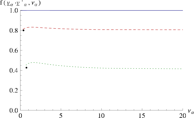
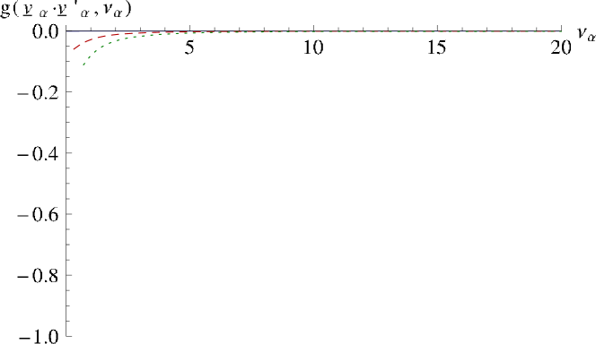
Figure 5.1: Physical and spurious electromagnetic form factors, $\tilde{f}(\underline{v}_{\alpha}\cdot\underline{v}_{\alpha}^{\prime},\nu_{\alpha})$ and $\tilde{g}(\underline{v}_{\alpha}\cdot\underline{v}_{\alpha}^{\prime},\nu_{\alpha})$, of a heavy-light pseudoscalar meson as a function of the modulus of the meson velocity $\nu_{\alpha}$ for different fixed values of $\underline{v}_{\alpha}\cdot\underline{v}_{\alpha}^{\prime}$ (1 solid, 1.2 dashed, 2 dotted). The black dots in the upper figure are the values for the Isgur-Wise function directly calculated in the Breit frame ($\nu_{\alpha}=u$).

5.1.4 The infinite momentum frame and the Breit frame

In order to get the Isgur-Wise function that depends on $\underline{v}_{\alpha}\cdot\underline{v}_{\alpha}^{\prime}$ alone we have to fix $\nu_{\alpha}$. There are two particular choices that lead to interesting consequences and that correspond to two particular reference frames. The first one is the infinite momentum frame, i.e. $\nu_{\alpha}\rightarrow\infty$, which has been already studied for finite masses in Chap. 4. The second one corresponds to the minimal possible value of $\nu_{\alpha}$ ($\nu_{\alpha}=u$), which is characteristic for the Breit frame.

The infinite-momentum frame

We have already observed that the $\nu_{\alpha}$-dependence of $\tilde{f}(\underline{v}_{\alpha}\cdot\underline{v}_{\alpha}^{\prime},\nu_{\alpha})$ as well as the spurious form factor $\tilde{g}(\underline{v}_{\alpha}\cdot\underline{v}_{\alpha}^{\prime},\nu_{\alpha})$ vanish quickly with increasing $\nu_{\alpha}$. It is thus suggestive to identify the Isgur-Wise function $\xi(\underline{v}_{\alpha}\cdot\underline{v}_{\alpha}^{\prime})$ with the limit $\nu_{\alpha}\to\infty$ of the physical form factor $\tilde{f}(\underline{v}_{\alpha}\cdot\underline{v}_{\alpha}^{\prime},\nu_{\alpha})$. This corresponds to the infinite-momentum frame (IF). In this limit the current acquires the expected structure

$$\tilde{J}^{\nu}_{\infty}(\vec{\underline{v}}_{\alpha}^{\prime},\vec{\underline{v}}_{\alpha})\stackrel{{\scriptstyle\nu_{\alpha}\rightarrow\infty}}{{\longrightarrow}}(\underline{v}_{\alpha}+\underline{v}_{\alpha}^{\prime})^{\nu}\,\xi_{\mathrm{IF}}(\underline{v}_{\alpha}\cdot\underline{v}_{\alpha}^{\prime})\,.$$ (5.17)

The Isgur-Wise function can be extracted from the non-vanishing components of the current

$$\xi_{\mathrm{IF}}(\underline{v}_{\alpha}\cdot\underline{v}_{\alpha}^{\prime})=\int\,\frac{d^{3}\tilde{k}_{\bar{q}}^{\prime}}{4\pi}\,\sqrt{\frac{\omega_{\tilde{k}_{\bar{q}}}}{\omega_{\tilde{k}^{\prime}_{\bar{q}}}}}\,\mathcal{S}_{\mathrm{IF}}\,\psi^{\ast}\,(|\vec{\tilde{k}}_{\bar{q}}^{\prime}|)\,\psi\,(|\vec{\tilde{k}}_{\bar{q}}|)\,\,.$$ (5.18)

$\mathcal{S}_{\text{IF}}$ is the spin rotation factor in this particular frame

$$\mathcal{S}_{\mathrm{IF}}=\frac{m_{\bar{q}}+\omega_{\tilde{k}^{\prime}_{\bar{q}}}+\tilde{k}^{\prime 1}_{\bar{q}}\,u}{\sqrt{(m_{\bar{q}}+\omega_{\tilde{k}_{\bar{q}}})(m_{\bar{q}}+\omega_{\tilde{k}^{\prime}_{\bar{q}}})}}\,.$$ (5.19)

$\tilde{k}^{\prime}_{\bar{q}}$ and $\tilde{k}_{\bar{q}}$ are related by Eq. (3.16) which, in the heavy-quark limit and for this particular kinematics, leads to the following relation between $\omega_{\tilde{k}_{\bar{q}}}$ and $\omega_{\tilde{k}^{\prime}_{\bar{q}}}$ (see boosts in App. C.1.1):

$$\omega_{\tilde{k}_{\bar{q}}}=2\tilde{k}^{\prime 1}_{\bar{q}}\,u+2\tilde{k}^{\prime 3}_{\bar{q}}\,u^{2}+\omega_{\tilde{k}^{\prime}_{\bar{q}}}(2u^{2}+1)\,.$$ (5.20)

The Breit frame

Another widely used frame to analyze the $\gamma^{\ast}M_{\alpha}\rightarrow M_{\alpha}$ subprocess is the Breit frame (B) in which the energy-transfer between the meson in the initial and the final states vanishes [7, 29]. It corresponds to the opposite situation of the infinite-momentum frame, since it is reached by taking the minimal value of $\nu_{\alpha}$, this is $\nu_{\alpha}^{2}=u^{2}=(\underline{v}_{\alpha}\cdot\underline{v}_{\alpha}^{\prime}-1)/2$ (cf. Eq. (5.7)). The structure of the current in this case is (see App. C.2):

$$\tilde{J}^{\nu}_{\infty}(\vec{\underline{v}}_{\alpha}^{\prime},\vec{\underline{v}}_{\alpha}) \stackrel{{\scriptstyle\nu_{\alpha}\rightarrow u}}{{\longrightarrow}} (\underline{v}_{\alpha}+\underline{v}_{\alpha}^{\prime})^{\nu}\,\Big{\{}\tilde{f}(\underline{v}_{\alpha}\cdot\underline{v}_{\alpha}^{\prime},\nu_{\alpha}=u)$$ (5.21)

$$+\sqrt{\frac{\underline{v}_{\alpha}\cdot\underline{v}_{\alpha}^{\prime}-1}{\underline{v}_{\alpha}\cdot\underline{v}_{\alpha}^{\prime}+1}}\,\tilde{g}(\underline{v}_{\alpha}\cdot\underline{v}_{\alpha}^{\prime},\nu_{\alpha}=u)\Big{\}}$$

$$=:(\underline{v}_{\alpha}+\underline{v}_{\alpha}^{\prime})^{\nu}\,\xi_{\mathrm{B}}(\underline{v}_{\alpha}\cdot\underline{v}_{\alpha}^{\prime}).$$

Since both covariants become proportional to $(\underline{v}_{\alpha}+\underline{v}_{\alpha}^{\prime})^{\nu}$, it is not possible to distinguish the physical and the spurious form factor. One is thus led to identify the Lorentz invariant quantity in Eq. (5.21) as the Isgur-Wise function obtained in the Breit (B) frame. The structure of $\xi_{\text{B}}(\underline{v}_{\alpha}\cdot\underline{v}_{\alpha}^{\prime})$ is the same as in Eq. (5.18)

$$\xi_{\mathrm{B}}(\underline{v}_{\alpha}\cdot\underline{v}_{\alpha}^{\prime})=\int\,\frac{d^{3}\tilde{k}_{\bar{q}}^{\prime}}{4\pi}\,\sqrt{\frac{\omega_{\tilde{k}_{\bar{q}}}}{\omega_{\tilde{k}^{\prime}_{\bar{q}}}}}\,\mathcal{S}_{\mathrm{B}}\,\psi^{\ast}\,(|\vec{\tilde{k}}_{\bar{q}}^{\prime}|)\,\psi\,(|\vec{\tilde{k}}_{\bar{q}}|)\,\,,$$ (5.22)

with the spin factor $\mathcal{S}_{\text{B}}$ being now

$$\mathcal{S}_{\mathrm{B}}=\frac{m_{\bar{q}}+\omega_{\tilde{k}^{\prime}_{\bar{q}}}+\tilde{k}^{\prime 1}_{\bar{q}}\,\frac{u}{\sqrt{u^{2}+1}}}{\sqrt{(m_{\bar{q}}+\omega_{\tilde{k}_{\bar{q}}})(m_{\bar{q}}+\omega_{\tilde{k}^{\prime}_{\bar{q}}})}}\,.$$ (5.23)

The difference between both frames resides in the relation between $\tilde{k}_{\bar{q}}^{\prime}$ and $\tilde{k}_{\bar{q}}$, which are connected by boosts, that are different in the Breit frame and the infinite-momentum frame (cf. App. C.2). Correspondingly

$$\omega_{\tilde{k}_{\bar{q}}}=2\tilde{k}^{\prime 1}_{\bar{q}}\,u\sqrt{u^{2}+1}+\omega_{\tilde{k}^{\prime}_{\bar{q}}}(2u^{2}+1).$$ (5.24)

Relating both reference frames

Despite the integrands in (5.18) and (5.22) are different, the numerical results for the integrals are found to be identical for $\xi_{\mathrm{B}}(\underline{v}_{\alpha}\cdot\underline{v}_{\alpha}^{\prime})$ and $\xi_{\mathrm{IF}}(\underline{v}_{\alpha}\cdot\underline{v}_{\alpha}^{\prime})$. This can be seen in Fig. 5.1, where the results for $\xi_{\mathrm{B}}(\underline{v}_{\alpha}\cdot\underline{v}_{\alpha}^{\prime})$ are indicated by black dots. The values for the dots coincide with the values for the curves for large $\nu_{\alpha}$.

It is thus suggestive to look for an analytical relation between $\xi_{\text{B}}(\underline{v}_{\alpha}\cdot\underline{v}_{\alpha}^{\prime})$ and $\xi_{\text{IF}}(\underline{v}_{\alpha}\cdot\underline{v}_{\alpha}^{\prime})$. One can indeed establish an analytical relation by a simple change of variables. The transformation turns out to be the following rotation:

$$\begin{pmatrix}\tilde{k}_{\bar{q}}^{\prime\,1}\\ \tilde{k}_{\bar{q}}^{\prime\,3}\end{pmatrix}_{\mathrm{IF}}=\frac{1}{\sqrt{u^{2}+1}}\begin{pmatrix}1&-u\\ u&1\end{pmatrix}\begin{pmatrix}\tilde{k}_{\bar{q}}^{\prime\,1}\\ \tilde{k}_{\bar{q}}^{\prime\,3}\end{pmatrix}_{\mathrm{B}}\,.$$ (5.25)

Applying this change of variables to the integrand in the infinite-momentum frame one obtains the same analytical result for the Isgur-Wise function as in the Breit frame. The conclusion is then that the Isgur-Wise function obtained by this procedure turns out to be the same irrespective of where it is computed, either in the Breit or in the infinite-momentum frame. This does not hold, however, for arbitrary frames (cf. Eq. (5.14) and Fig. 5.1), and it does not hold for finite mass of the heavy quark (cf. Figs. 4.1 and  4.2).

The Isgur-Wise function

The resulting Isgur-Wise function is thus the same irrespective of whether it is extracted in the Breit frame or in the infinite momentum frame. The subscripts “IF” and “B” will therefore not be taken into account any more. It will be more convenient for further purposes to use the analytical expression for the Isgur-Wise function obtained in the Breit frame. So we will take the following expression for the Isgur-Wise function in the sequel:

$$\xi(v\cdot v^{\prime})=\int\,\frac{d^{3}\tilde{k}_{\bar{q}}^{\prime}}{4\pi}\,\sqrt{\frac{\omega_{\tilde{k}_{\bar{q}}}}{\omega_{\tilde{k}^{\prime}_{\bar{q}}}}}\,\mathcal{S}\,\psi^{\ast}\,(|\vec{\tilde{k}}_{\bar{q}}^{\prime}|)\,\psi\,(|\vec{\tilde{k}}_{\bar{q}}|)\,\,,$$ (5.26)

with

$$\omega_{\tilde{k}_{\bar{q}}}=\tilde{k}^{\prime 1}_{\bar{q}}\,\sqrt{(v\cdot v^{\prime})^{2}-1}+\omega_{\tilde{k}^{\prime}_{\bar{q}}}\,(v\cdot v^{\prime})$$ (5.27)

and

$$\mathcal{S}=\frac{m_{\bar{q}}+\omega_{\tilde{k}^{\prime}_{\bar{q}}}+\tilde{k}^{\prime 1}_{\bar{q}}\,\sqrt{\frac{{(v\cdot v^{\prime})-1}}{{(v\cdot v^{\prime})+1}}}}{\sqrt{(m_{\bar{q}}+\omega_{\tilde{k}_{\bar{q}}})(m_{\bar{q}}+\omega_{\tilde{k}^{\prime}_{\bar{q}}})}}\,.$$ (5.28)

The underline and the subscript $\alpha$ have been dropped for simplicity. The Isgur-Wise function obtained within this procedure depends only on $v\cdot v^{\prime}$, has the correct normalization condition, i.e. $\xi(v\cdot v^{\prime}=1)=1$, and is independent of the heavy-quark mass. $\xi(v\cdot v^{\prime})$ is thus universal and the same for any meson that contains the same light antiquark. This property is called heavy-quark flavor symmetry and it is the first part of the proof that heavy-quark symmetry is respected by our approach.

5.2 Time-like momentum transfer

Until now we have studied for electron-meson scattering how heavy-quark symmetry arises sending the heavy-quark mass to infinity. In this way it disappears from the description, leading to a universal form factor, the Isgur-Wise function $\xi(v\cdot v^{\prime})$. Heavy-quark symmetry goes even further, it has also consequences for processes that involve time-like momentum transfers.

If matrix elements do not depend on the mass of the heavy quark, transition form factors that involve a change of flavor of the heavy quark are expected to be identical to those in which the flavor of the heavy quark is unaltered. One thus may expect relations between electromagnetic and weak form factors in the heavy-quark limit. Such relations are indeed given in the literature [8, 10]. They will be studied in the present section. As in the previous section, starting from the general expression for the form factors, the consequences of heavy-quark symmetry will be tested by taking the h.q.l. As we will see, both flavor symmetry and spin symmetry will occur in electroweak processes.

5.2.1 Kinematics in terms of velocities

For time-like momentum transfer the parametrization in terms of velocities $\underline{v}_{B}\cdot\underline{v}^{\prime}_{D^{(\ast)}}$ leads to the following meson and heavy-quark momenta (cf. Eqs. (4.15) and (4.16)):

$$\underline{k}_{B} = m_{B}\left(\begin{array}[]{c}1\\ 0\\ 0\\ 0\end{array}\right)=m_{B}\underline{v}_{B}\,,$$ (5.33)

$$\underline{k}_{D^{(\ast)}}^{\prime} = m_{D^{(\ast)}}\left(\begin{array}[]{c}\sqrt{(\underline{v}_{B}\cdot\underline{v}^{\prime}_{D^{(\ast)}})^{2}-1}\\ \underline{v}_{B}\cdot\underline{v}^{\prime}_{D^{(\ast)}}\\ 0\\ 0\end{array}\right)=m_{D^{(\ast)}}\underline{v}_{D^{(\ast)}}\,.$$ (5.38)

The (time-like) momentum transfer is given here by

$$0\leq\underline{q}^{2} = (\underline{k}_{B}-\underline{k}_{D^{(\ast)}})^{2}$$

$$=m_{B}^{2}+m_{D^{(\ast)}}^{2}-2m_{B}m_{D^{(\ast)}}\underline{v}_{B}\cdot\underline{v}^{\prime}_{D^{(\ast)}}\leq(m_{B}-m_{D^{(\ast)}})^{2}\,.$$

From Eqs. (5.33) and (5.2.1) one can deduce that $\underline{v}_{B}\cdot\underline{v}^{\prime}_{D^{(\ast)}}$ is restricted by the condition

$$1\leq\underline{v}_{B}\cdot\underline{v}^{\prime}_{D^{(\ast)}}\leq 1+\frac{(m_{B}-m_{D^{(\ast)}})^{2}}{2m_{B}m_{D^{(\ast)}}}\,.$$ (5.40)

Direct comparisons of form factors for space-like and time-like processes can be done within this interval.

5.2.2 Flavor symmetry

First we will study heavy-quark flavor symmetry by comparing the Isgur-Wise function (5.26) from electromagnetic scattering with the one from the $B\to De\bar{\nu}_{e}$ transition. Flavor symmetry predicts that in a $Q\bar{q}$-system the behavior of the light quark appears blind to the flavor of the heavy one. This implies that the form factors obtained for a system like $\bar{u}b$ should be identical to the ones obtained for $\bar{u}c$. Comparing the covariant structure of the electromagnetic and weak currents, (4.14) and (4.2) respectively, it can be demonstrated that the following relations should be fulfilled when the mass of the heavy quark goes to infinity [8, 10]

$$R\,\left[1-\frac{q^{2}}{(m_{B}+m_{D})^{2}}\right]^{-1}\,F_{0}(q^{2})\stackrel{{\scriptstyle\mathrm{h.q.l.}}}{{\longrightarrow}}\,\xi(\underline{v}_{B}\cdot\underline{v}^{\prime}_{D}),$$ (5.41)

$$R\,\,F_{1}(q^{2})\stackrel{{\scriptstyle\mathrm{h.q.l.}}}{{\longrightarrow}}\,\xi(\underline{v}_{B}\cdot\underline{v}^{\prime}_{D})\,,$$ (5.42)

with

$$R=\frac{2\sqrt{m_{B}m_{D}}}{m_{B}+m_{D}}\,.$$ (5.43)

and $\xi(\underline{v}_{B}\cdot\underline{v}^{\prime}_{D})$ being the h.q.l. of the electromagnetic form factor $F(Q^{2})$ (considered as function of $\underline{v}_{\alpha}\cdot\underline{v}_{\alpha}^{\prime}$).

5.2.3 Currents and form factors
in pseudoscalar-to-pseudoscalar meson transitions

The quark current (3.21) in the h.q.l. takes on the form

$$J^{\nu}_{B\rightarrow D}(\vec{\underline{k}}_{D}^{\prime},\vec{\underline{k}}_{B}) \stackrel{{\scriptstyle\mathrm{h.q.l.}}}{{\longrightarrow}} \sqrt{m_{B}m_{D}}\,\tilde{J}^{\nu}_{B\rightarrow D}(\vec{\underline{v}}_{D}^{\prime},\vec{\underline{v}}_{B})$$

$$= \sqrt{m_{B}m_{D}}\,\int\,\frac{d^{3}\tilde{k}_{\bar{q}}^{\prime}}{4\pi}\,\sqrt{\frac{\omega_{\tilde{k}_{\bar{q}}}}{\omega_{\tilde{k}^{\prime}_{\bar{q}}}}}\,\bigg{\{}\!\sum_{\mu_{b},\mu_{c}^{\prime}=\pm\frac{1}{2}}\!\!\!\bar{u}_{\mu_{c}^{\prime}}(\vec{\underline{v}}_{D}^{\,\prime})\,\gamma^{\nu}\,u_{\mu_{b}}(\vec{\underline{v}}_{B})$$

$$\times\frac{1}{2}\,D^{1/2}_{\mu_{b}\mu_{c}^{\prime}}\!\left[\!R_{\mathrm{W}}\!\left(\frac{\tilde{k}^{\prime}_{\bar{q}}}{m_{\bar{q}}},B_{c}(\underline{v}_{D}^{\prime})\right)\,\,\right]\bigg{\}}\,\psi^{\ast}\,(|\vec{\tilde{k}}_{\bar{q}}^{\prime}|)\,\psi\,(|\vec{\tilde{k}}_{\bar{q}}|)\,\,.$$

As in the electromagnetic case, the Wigner $D$-function that acts on the heavy-quark degrees of freedom becomes the unit matrix. The expression (5.2.3) is simpler than in the electromagnetic case due to the kinematics of the weak decay processes, where the initial state is at rest (cf. Sec. 3.2). This is the reason why the second Wigner rotation that depends on the initial velocity is absent here. When one imposes the condition $\underline{\vec{v}}_{\alpha}=0$ in the electromagnetic case (5.13) one recovers exactly Eq. (5.2.3). Note also that, due to the condition $\underline{\vec{v}}_{B}=0$, the kinematics resembles the one in the Breit frame, where the whole process also takes place only along one direction.

Using the properties of the Wigner $D$-functions one can write the point-like quark current as (cf. App. C.1.2):

$$\bar{u}_{\mu_{b}}(\vec{\underline{v}}_{D}^{\,\prime})\,\gamma^{\nu}\,u_{\mu_{b}}(\vec{\underline{v}}_{B})=\sqrt{\frac{2}{\underline{v}_{B}\cdot\underline{v}^{\prime}_{D}+1}}\,(\underline{v}_{B}+\underline{v}^{\prime}_{D})^{\nu}\,.$$ (5.45)

The meson transition current can therefore be expressed in terms of the covariant $(\underline{v}_{B}+\underline{v}^{\prime}_{D})^{\nu}$ alone:

$$\tilde{J}^{\nu}_{B\rightarrow D}(\vec{\underline{v}}_{D}^{\prime},\vec{\underline{v}}_{B})=(\underline{v}_{B}+\underline{v}^{\prime}_{D})^{\nu}\,\xi_{W}(\underline{v}_{B}\cdot\underline{v}^{\prime}_{D})\,.$$ (5.46)

The resulting analytical expression for $\xi_{W}(\underline{v}_{B}\cdot\underline{v}^{\prime}_{D})$ extracted in this manner from the semileptonic weak (‘$W$’) process is

$$\xi_{W}(\underline{v}_{B}\cdot\underline{v}_{D}^{\prime})=\int\,\frac{d^{3}\tilde{k}_{\bar{q}}^{\prime}}{4\pi}\,\sqrt{\frac{\omega_{\tilde{k}_{\bar{q}}}}{\omega_{\tilde{k}^{\prime}_{\bar{q}}}}}\,\mathcal{S}_{W}\,\psi^{\ast}\,(|\vec{\tilde{k}}_{\bar{q}}^{\prime}|)\,\psi\,(|\vec{\tilde{k}}_{\bar{q}}|)\,\,.$$ (5.47)

with

$$\omega_{\tilde{k}_{\bar{q}}}=\tilde{k}^{\prime 1}_{\bar{q}}\,\sqrt{(\underline{v}_{B}\cdot\underline{v}_{D}^{\prime})^{2}-1}+\omega_{\tilde{k}^{\prime}_{\bar{q}}}\,(\underline{v}_{B}\cdot\underline{v}_{D}^{\prime})$$ (5.48)

and

$$\mathcal{S}_{W}=\frac{m_{\bar{q}}+\omega_{\tilde{k}^{\prime}_{\bar{q}}}+\tilde{k}^{\prime 1}_{\bar{q}}\,\sqrt{\frac{{(\underline{v}_{B}\cdot\underline{v}_{D}^{\prime})-1}}{{(\underline{v}_{B}\cdot\underline{v}_{D}^{\prime})+1}}}}{\sqrt{(m_{\bar{q}}+\omega_{\tilde{k}_{\bar{q}}})(m_{\bar{q}}+\omega_{\tilde{k}^{\prime}_{\bar{q}}})}}\,.$$ (5.49)

The Isgur-Wise function for this weak heavy-to-heavy decay is thus identical with the one extracted from electron-meson scattering (cf. Eqs. (5.26)-(5.28)). This is an important result showing that the description of the electroweak structure of mesons is properly done within our approach. It guarantees heavy-quark flavor symmetry and provides the correct relations between space- and time-like form factors in the h.q.l.

5.2.4 Spin symmetry

Heavy-quark symmetry allows also to relate form factors involving pseudoscalar mesons with corresponding ones involving vector mesons in the h.q.l. This symmetry emerges from the decoupling of the heavy-quark spin. For weak pseudoscalar-to-vector transitions the form factors are related by [52]:

$$R^{\ast}\,\left[1-\frac{q^{2}}{(m_{B}+m_{D}^{\ast})^{2}}\right]^{-1}\,A_{1}(q^{2})\stackrel{{\scriptstyle\mathrm{h.q.l.}}}{{\longrightarrow}}\,\xi(\underline{v}_{B}\cdot\underline{v}^{\prime}_{D^{\ast}})\,,$$ (5.50)

$$R^{\ast}\,\,V(q^{2})\stackrel{{\scriptstyle\mathrm{h.q.l.}}}{{\longrightarrow}}\,\xi(\underline{v}_{B}\cdot\underline{v}^{\prime}_{D^{\ast}})\,,$$ (5.51)

and

$$R^{\ast}\,\,A_{i}(q^{2})\stackrel{{\scriptstyle\mathrm{h.q.l.}}}{{\longrightarrow}}\,\xi(\underline{v}_{B}\cdot\underline{v}^{\prime}_{D^{\ast}})\,,\quad i=0,2\,,$$ (5.52)

with

$$R^{\ast}=\frac{2\sqrt{m_{B}m_{D^{\ast}}}}{m_{B}+m_{D^{\ast}}}\,,$$ (5.53)

where the form factors $A_{i}(q^{2})$, $A_{1}(q^{2})$ and $V(q^{2})$ are those introduced in Eq. (4.2.2). In the following we will take as a representative example the $B\to D^{*}e\bar{\nu}_{e}$ transition.

5.2.5 Currents and form factors
in pseudoscalar-to-vector meson transitions

The weak transition current (3.2) becomes in the heavy quark limit

$$J^{\nu}_{B\rightarrow D^{\ast}} (\vec{\underline{k}}_{D^{\ast}}^{\prime},\underline{\mu}_{D^{\ast}}^{\prime};\vec{\underline{k}}_{B})\stackrel{{\scriptstyle\text{h.q.l.}}}{{\longrightarrow}}\sqrt{m_{B}m_{D}}\,\tilde{J}^{\nu}_{B\rightarrow D^{\ast}}(\vec{\underline{v}}_{D^{\ast}}^{\prime},\underline{\mu}_{D^{\ast}}^{\prime};\vec{\underline{v}}_{B})$$

$$=\sqrt{m_{B}m_{D}}\,\int\,\frac{d^{3}\tilde{k}_{\bar{q}}^{\prime}}{4\pi}\,\sqrt{\frac{\omega_{\tilde{k}_{\bar{q}}}}{\omega_{\tilde{k}^{\prime}_{\bar{q}}}}}\,\bigg{\{}\!\sum_{\mu_{b},\mu_{c}^{\prime},\tilde{\mu}_{\bar{q}}^{\prime}=\pm\frac{1}{2}}\!\!\!\!\!\!\bar{q}_{\mu_{c}^{\prime}}(\underline{\vec{v}}_{D^{\ast}}^{\prime})\,\gamma^{\nu}\,(1-\gamma^{5})u_{\mu_{b}}(\underline{\vec{v}}_{B})$$

$$\times\sqrt{2}(-1)^{\frac{1}{2}-\mu_{b}}C^{1\underline{\mu}^{\prime}_{\!D^{\ast}}}_{\frac{1}{2}\mu_{c}^{\prime}\frac{1}{2}\tilde{\mu}_{\bar{q}}^{\prime}}\,$$

$$\times D^{1/2}_{\tilde{\mu}_{\bar{q}}^{\prime}-\mu_{b}}\!\left[\!R^{-1}_{\mathrm{W}}\!\left(\frac{\tilde{k}^{\prime}_{\bar{q}}}{m_{\bar{q}}},B^{-1}_{c}(\underline{v}_{D^{\ast}}^{\prime})\right)\right]\bigg{\}}\,\psi^{\ast}_{D^{\ast}}\,(|\vec{\tilde{k}}_{\bar{q}}^{\prime}|)\,\psi_{B}\,(|\vec{\tilde{k}}_{\bar{q}}|)\,.$$ (5.54)

In the h.q.l. the covariant structure of (4.2.2) goes over into

$$\tilde{J}^{\nu}_{B\rightarrow D^{\ast}}(\vec{\underline{v}}_{D^{\ast}}^{\prime},\underline{\mu}_{D^{\ast}}^{\prime};\vec{\underline{v}}_{B}) = i\,\epsilon^{\nu\alpha\beta\gamma}\,\epsilon_{\alpha}(m_{D^{\ast}}\vec{\underline{v}}_{D^{\ast}}^{\prime},\underline{\mu}_{D^{\ast}}^{\prime})\,\underline{v}^{\prime}_{D^{\ast}\beta}\,\underline{v}_{B\gamma}\,\xi(\underline{v}_{B}\cdot\underline{v}^{\prime}_{D^{\ast}})\,$$

$$-\Big{[}\epsilon^{\nu}(m_{D^{\ast}}\vec{\underline{v}}_{D^{\ast}}^{\prime},\underline{\mu}_{D^{\ast}}^{\prime})\,(\underline{v}_{B}\cdot\underline{v}^{\prime}_{D^{\ast}}+1)$$

$$\qquad-\underline{v}^{\prime\nu}_{D^{\ast}}\,\epsilon(m_{D^{\ast}}\vec{\underline{v}}_{D^{\ast}}^{\prime},\underline{\mu}_{D^{\ast}}^{\prime})\cdot\underline{v}_{B}\Big{]}\,\xi(\underline{v}_{B}\cdot\underline{v}^{\prime}_{D^{\ast}})\,.$$

By comparison of Eqs. (5.2.5) and (5.2.5) one can see that the Isgur-Wise function $\xi(\underline{v}_{B}\cdot\underline{v}^{\prime}_{D^{\ast}})$ is the same as in Eqs. (5.47)-(5.49). This shows how heavy-quark spin symmetry, which has its origin in the decoupling of the heavy-quark spin from the spin of the light degrees of freedom, arises when the mass goes to infinity. This proves that heavy-quark spin symmetry is also respected by our approach.

In the next chapter numerical results for the Isgur-Wise function will be presented and compared with results for the case of finite heavy-quark masses. Heavy-quark symmetry breaking due to finite masses will be discussed.

Chapter 6 Numerical studies I

In this chapter we will study the electroweak (transition) form factors of heavy-light mesons numerically. By comparing the numerical results for these form factors, obtained with physical masses for the heavy quarks, with the outcome in the heavy-quark limit, we will estimate the amount of heavy-quark-symmetry breaking for the physical masses.

6.1 Meson wave function

The form factors, and thus the Isgur-Wise function, are solely determined by the $Q\bar{q}$ bound-state wave function and the constituent masses. We take a harmonic-oscillator wave function which is defined as follows:

$$\psi(\kappa)=\frac{2}{\pi^{\frac{1}{4}}a^{\frac{3}{2}}}\exp\left(-\frac{\kappa^{2}}{2a^{2}}\right)\,.$$ (6.1)

There are mainly two reasons for choosing such a simple wave function. On the one hand it is the main goal of this work to demonstrate that the kind of relativistic coupled-channel approach we are using is general enough to provide sensible results for the description of the electroweak structure of heavy-light systems. We do not want to give quantitative predictions for electroweak form factors based on sophisticated constituent-quark models. On the other hand this wave function will allow to do a direct comparison with analogous calculations carried out within a front-form approach [34]. The numerical calculations could, of course, be carried out using any other model wave function obtained from a particular bound-state problem. The numerical results presented in this chapter have been computed using the model parameters quoted in Table 6.1, which have been taken from Ref. [34].

$m_{u,d}$	$m_{b}$	$m_{c}$	$a$
0.25 GeV	4.8 GeV	1.6 GeV	0.55 GeV

Table 6.1: Model parameters used for the numerical calculations presented in this chapter. Physical masses as well as the harmonic-oscillator parameter $a$ are taken from Ref. [34]. The Cabibbo-Kobayashi-Maskawa matrix element $|V_{cb}|$ as well as the physical meson masses are the actual values quoted by the Particle Data Group [57].

6.2 The Isgur-Wise function

The solid line in Fig. 6.1 shows the numerical result for the Isgur-Wise function as derived in Sec. 5.1.4. The result is the same for the electromagnetic case computed either in the Breit frame or in the infinite-momentum frame and agrees also with the one for weak decays, despite those processes involve space- and time-like momentum transfers, respectively. Our numerical result coincides with the Isgur-Wise function obtained within the light-front quark model of Ref. [34]. The dashed line corresponds to spin-rotation factor $\mathcal{S}=1$; this is the result one would have for spinless quarks. The difference between both lines indicates the importance of the appropriate treatment of relativistic spin rotations when boosting the initial to the final $Q\bar{q}$-bound-state wave function.

A comparison with experimental data will be done later when we present form-factor results for finite heavy-quark masses. The Isgur-Wise function will then be used as a reference quantity to estimate the amount of heavy-quark symmetry breaking.

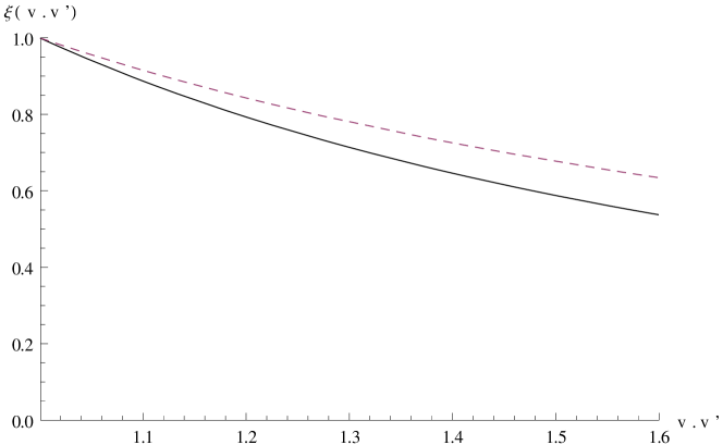
Figure 6.1: The Isgur-Wise function (solid line) as given in Eqs. (5.26)-(5.28) with the model parameters of Table 6.1. The dashed line corresponds to spin-rotation factor $\mathcal{S}=1$.

6.3 Heavy-quark symmetry breaking
in electromagnetic processes

Heavy-quark symmetry is broken for finite heavy-quark masses. Form factors of heavy-light mesons differ from the Isgur-Wise function since the physical masses are finite. Once the Isgur-Wise function has been obtained, it can be used to estimate quantitatively to which extend the realistic case, corresponding to physical masses, deviates from the heavy-quark limit. This gives us an estimate of the amount of heavy-quark symmetry breaking and provides conditions under which the heavy-quark limit turns out to be a good approximation.

Fig. 6.2 shows the electromagnetic form factors for the $D^{+}$ and $B^{-}$ mesons, as measured in the space-like momentum transfer region, as functions of $v\cdot v^{\prime}$. They have to be compared with the Isgur-Wise function (solid line) which is normalized to the charge of the heavy quark in each case. The electromagnetic form factor is the result of the sum of two contributions that correspond to the photon coupling to the heavy and to the light quarks (cf. Eq. 3.1). Each of them is weighted with the charge of the corresponding quark. In the heavy-quark limit the contribution in which the light quark is active vanishes. For finite heavy-quark masses it causes a peak at $v\cdot v^{\prime}\to 1$, which becomes more pronounced with increasing the mass of the heavy quark and disappears completely in the heavy-quark limit, since the light-quark contribution decreases faster with increasing $v\cdot v^{\prime}$ than the heavy-quark contribution. In case of the $B⁻$ meson (bottom) the light-quark contribution dies out rather fast, such that nearly the whole form factor is dominated by the heavy-quark contribution. It lies above the Isgur-Wise function, being about 20% larger. The heavy-quark contribution starts to dominate at $v\cdot v^{\prime}\gtrsim 1.1$ in this case (which corresponds to $\text{Q}^{2}\gtrsim 5$ GeV²).

In the case of the $D^{+}$-meson the dominance of the heavy-quark contribution sets in at about the same momentum transfer ($\text{Q}^{2}\gtrsim 5$ GeV²), which corresponds to (cf. Eq. (5.2.1)) $v\cdot v^{\prime}\gtrsim 1.7$. The absolute magnitude of the form factor at $v\cdot v^{\prime}\sim 2$ deviates from the Isgur-Wise function by abot 60%. This is due to the smallness of the charm-quark mass. For the $B^{-}$ meson the heavy-quark limit thus seems to be a reasonable approximation whereas the charm quark mass is obviously too small to be well approximated by the heavy-quark limit.

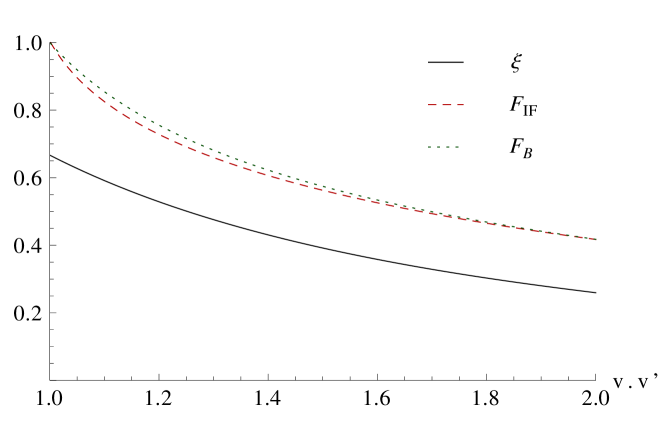
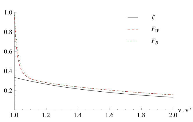
Figure 6.2: Electromagnetic form factors of the $D^{+}$ (top) and $B^{-}$ (down) mesons calculated in the Breit frame (dotted line) and infinite-momentum frame (dashed line) in comparison with the Isgur-Wise function (solid line). For direct comparison the Isgur-Wise function is multiplied by $|\mathcal{Q}_{Q}|$, i.e. the charge of the heavy quark. Model parameters are taken from Table 6.1.

6.4 Heavy-quark symmetry breaking
in weak processes

In the following, numerical results for the weak form factors as measured in the $B^{-}\to D^{0}e^{-}\bar{\nu}_{e}$ and $B^{-}\to D^{0(*)}e^{-}\bar{\nu}_{e}$ decay processes will be discussed.

Heavy-quark flavor symmetry breaking

In order to test heavy-quark flavor symmetry numerically and to see how its breaking takes place, we calculate the decay form factors for finite masses of the heavy quarks (cf. Table 6.1). Starting from the physical values for the quark masses, it can be tested numerically how heavy-quark symmetry arises by scaling up $m_{b}$ and $m_{c}$. Fig. 6.3 shows the $F_{1}$ and $F_{0}$ form factors that can be measured in the $B^{-}\to D^{0}e^{-}\bar{\nu}_{e}$ decay, for physical values of $m_{b}$ and $m_{c}$ and values that are about 6 times larger. The form factors are multiplied by the corresponding kinematical factors that relate them to the Isgur-Wise function (cf. (5.41)-(5.43)). The deviation from the Isgur-Wise function indicates the amount of heavy-quark symmetry breaking. As it was shown analytically, heavy-quark symmetry predicts that the quantities $RF_{1}$ and $R(1-q^{2}/(m_{B}+m_{D})^{2})^{-1}F_{0}$ agree in the heavy-quark limit and they go over into the Isgur-Wise function. Taking the physical masses of the heavy quarks the differences between the resulting quantities turn out to be less than 7% of their absolute values and they become smaller with increasing $v\cdot v^{\prime}$ (cf. Fig 6.3 (top)). the deviation from the Isgur-wise function, however, is about 15%.

Taking $b$- and $c$-masses 6.25 times larger than the physical masses (which means $m_{c}=10$ GeV), $RF_{1}$ and $R(1-q^{2}/(m_{B}+m_{D})^{2})^{-1}F_{0}$ are already much closer to the Isgur-Wise function (cf. Fig 6.3, bottom). The discrepancy between $RF_{1}$, $R(1-q^{2}/(m_{B}+m_{D})^{2})^{-1}F_{0}$ and $\xi(v\cdot v^{\prime})$ is in this case less than 10%.

Heavy-quark spin symmetry breaking

Analogously to heavy-quark flavor symmetry, heavy-quark spin symmetry can be also tested numerically. Fig. 6.4 shows how the form factors, multiplied by appropriate kinematical factors given by the relations (5.50)-(5.53) approach the Isgur-Wise function by increasing the heavy-quark mass.

The prediction is that $R^{*}V$, $R^{*}A_{0}$, $R^{*}A_{2}$ and $R^{*}(1-q^{/}(m_{B}+m_{D^{*}})^{2})^{-1}A_{1}$ coincide with the Isgur-Wise function in the heavy-quark limit. These quantities are shown in Fig. 6.4 (top) for physical masses (cf. Table 6.1). The maximum difference between them are about 5% and they differ from the Isgur-Wise function by about 20%. In order to see numerically the restoration of heavy-quark symmetry for large masses the form factors (multiplied by the corresponding kinematical factors) are plotted in Fig. 6.4 (down) for $b$- and $c$- masses of about one order of magnitude larger, so that $m_{c}=10$ GeV.

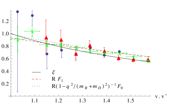
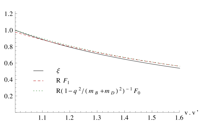
Figure 6.3: Top: weak $B^{-}\rightarrow D^{0}$ decay form factors (multiplied by appropriate kinematical factors, cf. (5.41) - (5.43)) for physical heavy-quark masses in comparison with the Isgur-Wise function. Experimental data have been taken from Belle [54] (dots), CLEO [55] (triangles) and BABAR [56] (crosses) assuming that $|V_{cb}|=0.0409$, i.e. the central value given by the Particle Data Group [57]. Model parameters are taken from Table 6.1. Bottom: $c$ and $b$-quark masses are multiplied by a factor $6.25$ such that $m_{c}=10$ GeV and meson masses are taken equal to the corresponding quark masses.

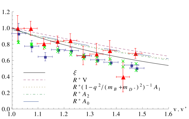
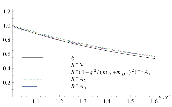
Figure 6.4: Top: weak $B^{-}\rightarrow D^{0\ast}$ decay form factors (multiplied by appropriate kinematical factors, cf. (5.50) - (5.53)) for physical heavy-quark masses in comparison with the Isgur-Wise function. Model parameters are taken from Table 6.1. Experimental data have been taken from Belle [58] (dots), CLEO [59] (triangles) and BABAR [60] (crosses) assuming that $|V_{cb}|=0.0409$, i.e. the central value given by the Particle Data Group [57]. In the lower figure $c$ and $b$-quark masses are multiplied by a factor $6.25$ such that $m_{c}=10$ GeV and meson masses are taken equal to the corresponding quark masses.

Other observables

The quantity that can be directly extracted experimentally from the (unpolarized) semileptonic decay rate, $d\Gamma_{B\to De\bar{\nu}}/d\omega\propto(\omega^{2}-1)^{3/2}|V_{cb}|^{2}|F_{D}(\omega)|^{2}$, is $V_{cb}F_{D}(\omega):=V_{cb}RF_{1}(q^{2}(\omega))$, with $\omega:=v\cdot v^{\prime}$. Results measured in Refs. [54, 55, 56] are plotted in Fig. 6.3 divided by the current value of $V_{cb}$. They can be compared with this model predictions (dashed line). The simple harmonic-oscillator model reproduces the experiments reasonably well and they are comparable with other constituent quark models [35, 38]. The resulting branching ratio is in good agreement with experiment:

$$BR(B^{0}\to D^{+}l^{-}\nu_{l}) = 2.3\%,$$ (6.2)

$$BR^{\text{exp}}(B^{0}\to D^{+}l^{-}\nu_{l}) = (2.18\pm 0.12)\%.$$ (6.3)

Other quantities that characterize the process are the value of $F_{D}$ at zero recoil, i.e. $F_{D}(\omega=1)=RF_{1}(\omega=1)$ and the slope at zero recoil $\rho^{2}_{D}:=-F^{\prime}_{D}(\omega=1)/F_{D}(\omega=1)$. The results obtained within the present model are

$$F_{D}(\omega=1) = 0.93,$$ (6.4)

$$\rho^{2}_{D} = 0.59.$$ (6.5)

It is interesting to look at these values in the heavy-quark limit. $F_{D}(\omega)$ goes over into $\xi(\omega)$ in the h.q.l., so its value at zero recoil is obviously 1. The slope becomes then $\rho^{2}:=-\xi^{\prime}_{D}(\omega=1)=1.24$. The result differs considerably from the corresponding one for physical masses of the heavy quarks. The experimental value, as quoted by the Heavy Flavor Averaging Group [61] is

$$\rho^{2}_{D}=1.18\pm 0.06,$$ (6.6)

which is closer to the result of the model in the h.q.l.

Remarks

For the discussion presented above we have used the same harmonic-oscillator wave function with oscillator parameter $a=0.55$ GeV, for both the $B^{-}$ and $D^{*}$ mesons. Any flavor dependence in the wave function has been ignored. It has been deliberately done in this way for the purpose of studying those effects that are exclusively consequences of heavy quark symmetry breaking due to taking the masses of the heavy quarks finite. Any kind of flavor dependence in the wave function, as it could be for example, a different oscillator parameter for each meson, would have influenced the numerical results. For instance, taking $a_{D}=0.465$ GeV as it is suggested in a front-form analysis of heavy-meson decay constants [62], while keeping $a_{B}=0.55$ GeV, the result for the slope at zero recoil would have been $\rho^{2}_{D}=0.65$, which is about 10% larger than the one obtained for $a_{B}=a_{D}=0.55$ GeV.

6.4.1 Cluster properties

Let us discuss now the spurious dependencies that appear in the form factors due to wrong cluster properties inherent in the Bakamjian-Thomas construction. The Mandelstam-$s$ dependence does not spoil the Poincaré invariance of the 1-photon-exchange amplitude, it is rather a consequence of the non-local character of the photon-meson vertex. If one considered the $\gamma^{*}M\to M$ subprocess only, the $s$-dependence could be interpreted as a frame dependence in the description of the subprocess. We have seen that there are two special reference frames (for $\gamma^{*}M\to M$), corresponding to two particular values of $s$. Namely, the minimum $s$ to reach a particular momentum transfer $\text{Q}^{2}$ and $s\to\infty$ (with $\text{Q}^{2}$ fixed). They have been called the Breit frame and the infinite-momentum frame, respectively. We have shown (cf. Sec. 5.1.4) that in both cases the covariant structure of the current can be expressed in terms of physical meson covariants only. In Fig. 6.2 the electromagnetic form factors for the $D^{+}$ and $B^{-}$ mesons computed in these two particular reference frames are shown. The difference between the Breit-frame result and the infinite-momentum-frame result is determined by the ratio $m_{Q}^{2}/\text{Q}^{2}$. In both frames the form factors at $\text{Q}^{2}=0$ are normalized to 1. Therefore the Breit-frame result tends to approach the infinite-momentum-frame result faster for the light $D^{+}$-meson than for the $B^{-}$-meson.

6.5 Comparison with front-form results

There are several calculations that have been done in a front-form approach to which the analytical and numerical results presented here can be compared. Ref. [34], where the model parameters have been taken from, provides two different analytical expressions corresponding to two different wave function models, namely a Gaussian-type one and the flavor dependent Wirbel-Stech-Bauer wave function [50]. The Isgur-Wise functions in [34] are obtained by taking the heavy-quark limit of the form factors of the $B\to D$ and $B\to D^{*}$ decays. The authors obtain the same numerical result for the Isgur-Wise function in the $B\to D$ and $B\to D^{*}$ processes when using a Gaussian wave function. However, their result turns out to be different when using a flavor dependent Wirbel-Stech-Bauer wave function [50]. Their conclusion is thus that the Wirbel-Stech-Bauer wave function does not preserve heavy-quark symmetry. In this work we have used the Gaussian wave function type and the numerical result for the Isgur-Wise function turns out to be identical to the one of Ref. [34]. The value of the slope at zero recoil is also found to be the same, $\rho^{2}=-\xi^{\prime}(1)=1.24$.

Unlike in the case of systems of equal constituent masses [20, 21], where the equivalence between point- and front-form results was already shown analytically for electromagnetic form factors, such an equivalence is not easy to establish analytically for heavy-light systems in the heavy-quark limit. There are, however, several hints suggesting that the equivalence may hold also in this case. In the case of the pion, the analytical result for the form factor for space-like momentum transfers was shown to be identical to the front-form expression that results from the +-component of a one-body current in the $q^{+}=0$ frame [20]. If such an equivalence extended to the case of unequal masses and generalized at least to those electroweak transition form factors that are not affected by $Z$-graphs contributions, the heavy-quark limit of electroweak heavy-light meson (transition) form factors in the point form should lead to the same Isgur-Wise function as the front-form approach. We see this numerically, but we have not attempted to establish the relation analytically so far.

Derivations of the Isgur-Wise function carried out within a front-form approach in, e.g. [34, 53], used as a starting point the weak transition form factor, which is extracted in the time-like momentum transfer region. In order to do calculations that involve time-like momentum transfers it is necessary to give up the $q^{+}=0$ condition and consequently the absence of $Z$-graphs is not guaranteed any more. This is confirmed by an analysis of the triangle diagram for $B\to D^{(*)}$ decays within a simple covariant model [37]. In Ref. [37] it is demonstrated that computing the weak form factors for $\bar{\nu}_{e}B\to eD^{(*)}$ scattering in a $q^{+}=0$ frame and applying an analytical continuation ($q_{\perp}\to iq_{\perp}$) in order to go to the time-like momentum transfer region is equivalent to computing the decay form factors in the time-like momentum transfer region (where $q^{+}\neq 0$), provided that the $Z$-graph contributions are appropriately taken into account. The importance of the $Z$-graph contributions decreases when increasing the mass of the heavy quark and vanishes completely in the heavy-quark limit. This is due to the impossibility of creating an infinitely heavy quark-antiquark pair out of the vacuum.

For finite masses we obtain results for the weak $M\to M^{\prime}$ decay form factors which differ from those obtained within the front-form approach. Fig. 6.5 may also provide a hint at the importance of the $Z$-graph contributions for finite masses when computing in $q^{+}\neq 0$ frames. Part of the discrepancies between the form factors extracted in the infinite-momentum frame and in the Breit frame may be attributed to missing $Z$-graph contributions in the Breit frame [36].

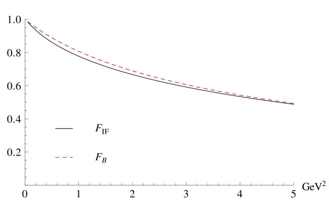
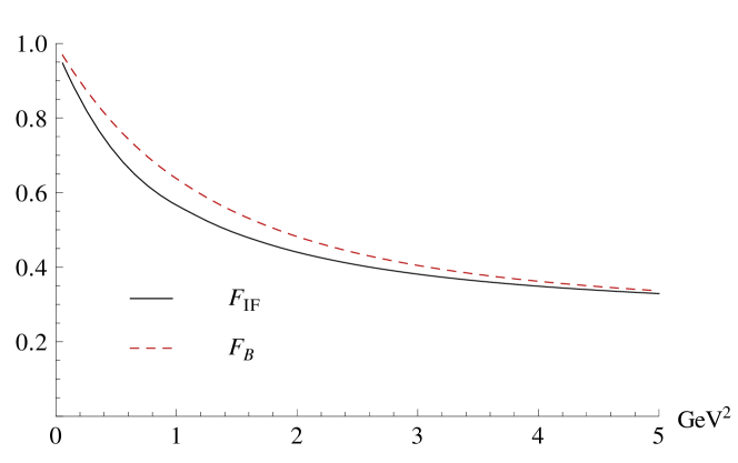
Figure 6.5: Electromagnetic form factor of the $D^{+}$ (top) and $B^{-}$ (bottom) mesons calculated in the Breit (B) and infinite-momentum (IF) frames as a function of the (space-like) 4-momentum transfer squared $\text{Q}^{2}=-q^{2}$. Model parameters are taken from Table 6.1.

Chapter 7 Numerical studies II

7.1 Introduction

In the previous chapter the numerical calculations where focused on the study of heavy-quark symmetry as well as on cluster-separability properties of our point-form approach. For that purpose the same harmonic-oscillator wave function with parameter $a=0.55$ GeV was used for all numerical studies. In this chapter we introduce a flavor dependence in the wave function, by assuming a different harmonic oscillator parameter for each meson. We will extract the form factors for several semileptonic decays, both for heavy-to-heavy and for heavy-to-light transitions, as a function of the 4-momentum transfer squared, i.e. $F_{0}(q^{2})$ and $F_{1}(q^{2})$ in the pseudoscalar-to-pseudoscalar case, and $V(q^{2})$, $A_{0}(q^{2})$, $A_{1}(q^{2})$ and $A_{2}(q^{2})$ in the pseudoscalar-to-vector case.

Even taking into account this flavor dependence, the model remains very simple. It is certainly not sophisticated enough to establish quantitative predictions which could be compared with experiments. Nonetheless, it is worth carrying out such calculations for several decays in order to see how our approach compares with other approaches and to learn at least qualitatively how the transition form factors depend on the kind of transition considered. We are particularly interested in comparisons with front-form results and the role of non-valence contributions in the description of currents and form factors. In front-form such non-valence contributions turn out to become important when one goes from space-like to time-like momentum transfers and they may play a role in our approach as well. As mentioned already in Sec. 6.5, for time-like momentum transfer it is not possible to use the $q^{+}=0$ frame in front form. As a consequence non-valence configurations leading to $Z$-graph contributions (quark-antiquark pairs created from the vacuum) can occur. Such $Z$-graph contributions have been analyzed in Ref. [37]. Applying analytic continuation ($q_{\perp}\to iq_{\perp}$) from the space-like to the time-like momentum transfer region to transition form factors calculated in a $q^{+}=0$ frame for space-like momentum transfers it is shown that the outcome is the same as the result from a direct calculation of the decay form factors in the time-like region (where $q^{+}\neq 0$), provided that the $Z$-graph contributions are appropriately taken into account. The importance of the $Z$-graph contributions decreases with increasing the mass of the heavy quark and it vanishes in the heavy-quark limit, since an infinitely heavy quark-antiquark pair cannot be produced out of the vacuum. Our numerical values for the Isgur-Wise function agree with those obtained within a front form quark model [34]. As soon as the decay form factors are calculated for finite physical masses of the heavy quarks, differences between the point- and front-form approach appear. These differences may be attributed to the different roles played by $Z$-graphs in either approach.

The major aim of this chapter is to provide the numerical results for time-like form factors using identical parameters and wave functions as in Ref. [34] (they are quoted in Table 7.1) and perform a numerical comparison of our point-form approach with the front-form one.

A second issue we would like to address with these comparisons concerns the frame dependence that appears in the calculation of form factors of pseudoscalar-to-vector transitions in the front-form approach. In the light-front quark model of Ref. [34], for instance, the authors choose a frame in which the momentum transfer is purely longitudinal, i.e. $q_{\perp}=0$, $q^{2}=q^{+}q^{-}$. Working in this way, form factors of processes that involve vector mesons, cannot be extracted unambiguously, and the form factors exhibit a dependence on whether the daughter meson goes in the positive or negative $z$-direction. We, on the other hand, showed in Chap. 4 that in our case there is no frame dependence of the form factors and they can be determined without any ambiguity from the different components of the current. This will be discussed Sec. 7.3.

$a_{\pi}$	$a_{\rho}$	$a_{K}$	$a_{K^{*}}$	$a_{D}$	$a_{D^{*}}$	$a_{B}$	$a_{B^{*}}$
0.33	0.30	0.38	0.31	0.46	0.47	0.55	0.55

Table 7.1: Harmonic-oscillator parameters (in GeV) for the meson wave functions used for the calculation of transition form factor in this chapter. They have been taken from Ref. [34] where they were determined by fitting the wave functions to the experimental values for the decay constants.

7.2 Pseudoscalar-to-pseudoscalar transitions

For pseudoscalar-to-pseudoscalar transitions, in order to allow for comparison with other work, besides $F_{0}(q^{2})(=f_{+}(q^{2}))$ and $F_{1}(q^{2})$, also $f_{-}(q^{2})$ is depicted for all computed decays. $f_{-}(q^{2})$ and $f_{+}(q^{2})$ are defined by

$$J^{\mu}(p_{1},p_{2})=f_{+}(q^{2})(p_{1}+p_{2})^{\mu}+f_{-}(q^{2})(p_{1}-p_{2})^{\mu},$$ (7.1)

where $p_{1}$ and $p_{2}$ are the initial and final meson 4-momenta. Their relation with $F_{0}(q^{2})$ and $F_{1}(q^{2})$ is given by (cf. Sec. 4.2.1):

$$F_{1}(q^{2})=f_{+}(q^{2}),\qquad F_{0}(q^{2})=f_{+}(q^{2})+\frac{q^{2}}{M_{1}^{2}-M_{2}^{2}}f_{-}(q^{2}).$$ (7.2)

The values at $q^{2}=0$ for $F_{1}(0)$, or equivalently for $f_{+}(0)$, are shown in Table 7.2 together with the results obtained within the light-front quark model [34]. For heavy-to-heavy transitions, i.e. $B\to D$, as well as for $B\to\pi(K)$ transitions both, front-form and point-form results, seem to agree quite well, whereas they differ slightly for $D\to\pi(K)$.

We do not have a definitive explanation for this fact, but we suspect that these differences are due to the different way in which $Z$-graphs enter the form factors in either approach. There is a particular frame, namely the $q^{+}=0$ frame, in the front form, where $Z$-graphs disappear. In point form a particular $q^{+}=0$ frame can be realized for lepton-hadron scattering by taking the limit of infinite large Mandelstam $s$, which corresponds to the infinite-momentum frame of the hadron. This explains, e.g., the equality of our point-form results for electromagnetic meson form factors (for $q^{2}<0$) with corresponding front-form results. In the $q^{+}=0$ frame however, weak decays cannot take place, since the process is necessarily time-like ($q^{2}=q^{+}q^{-}-q_{\perp}>0$) or light-like at the point for maximal recoil ($q^{2}=0$). In the light-front quark model of Ref. [34], the calculations are done in a frame where the momentum transfer is purely longitudinal, this is $q_{\perp}=0$, $q^{2}=q^{+}q^{-}$. At $q^{2}=0$ either $q^{+}$ or $q^{-}$ must vanish which corresponds to the daughter meson going either in + or in $-$ $z$-direction, respectively. Since the pseudoscalar decay form factors do not depend on whether the daughter meson goes into + or $-$ $z$-direction one can assume $q^{+}=0$. This implies, however, that $Z$-contributions vanish at the maximum recoil point. For $q^{2}>0$ there is, however, no argument to exclude $Z$-graph contributions in the decay form factors. In point form one does not even have an argument at $q^{+}=0$ (apart of the mass of the produced $Q\bar{Q}$-pair) that $Z$-graphs should vanish.

As in Ref. [34], a quantitative estimate of the $Z$-graph contribution is not within the scope of this work. We have seen, however, in the previous section that the point-form results reproduce the front-form ones exactly in the heavy-quark limit. The reason is that in these $Z$-graph contributions vanish, since it is not possible to create a infinitely heavy $Q\bar{Q}$-pair out of the vacuum. One can therefore expect that for heavy-to-heavy transitions point-form and front-form results show a greater resemblance than for heavy-to-light transitions. For heavy-to-light processes non-valence contributions are expected to be more important. It is thus not surprising that the results differ in both approaches. In the $D\to K$ and $D\to\pi$ cases, point- and front-form results differ considerably, the front-form results being somewhat closer to the experimental data [57].

Another resemblance with the front-form results is that $f_{-}(q^{2})\sim-f_{+}(q^{2})$ for $B\to\pi$ and to less extend for $D\to\pi$ (cf. Figs. 7.2 and 7.3). Near zero recoil (where $q^{2}$ is maximum) heavy-quark symmetry predicts $(f_{+}+f_{-})^{B(D)\pi}\sim\frac{1}{\sqrt{m_{B(D)}}}$. In our case we rather have

$$(f_{+}+f_{-})^{B\pi}_{q_{\text{max}}}\sim 0.22,\qquad(f_{+}+f_{-})^{D\pi}_{q_{\text{max}}}\sim 0.43,$$ (7.3)

whereas $1/\sqrt{m_{B}}\sim 0.43$ and $1/\sqrt{m_{D}}\sim 0.73$. Like in front form these kind of relations are badly violated for $B(D)\to K$.

	Front form [34]	Point form (this work)	Experiment [57]
$B\to D$	0.70	0.68
$B\to\pi$	0.26	0.26
$B\to K$	0.34	0.34
$D\to\pi$	0.64	0.58	0.661$\pm$0.022
$D\to K$	0.75	0.70	0.727$\pm$0.011

Table 7.2: $F_{1}(0)$ (or equivalently $f_{+}(0)$) form factor for pseudoscalar-to-pseudoscalar transitions, corresponding to Figs. 7.1 - 7.3.

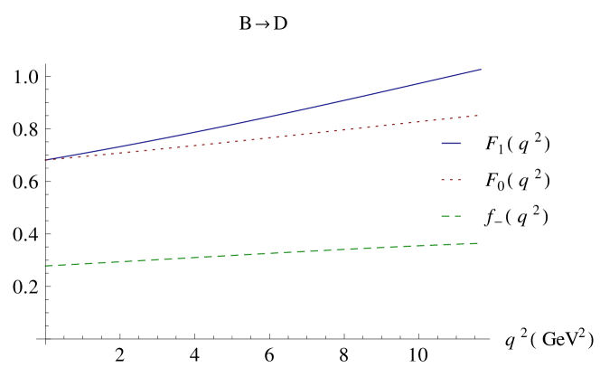
Figure 7.1: $B\to D$ transition form factors in the whole range $0\leq q^{2}\leq(M_{B}-M_{D})^{2}$. Parameters for the quark masses and harmonic-oscillator wave functions are taken from Tables 6.1 and 7.1, respectively. For the meson masses the current values given by the Particle Data Group have been taken [57].

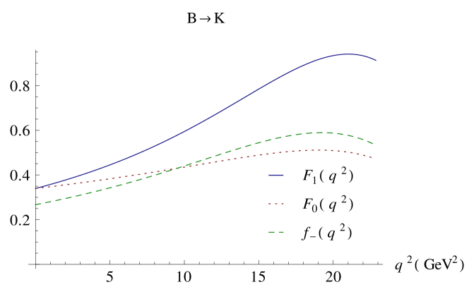
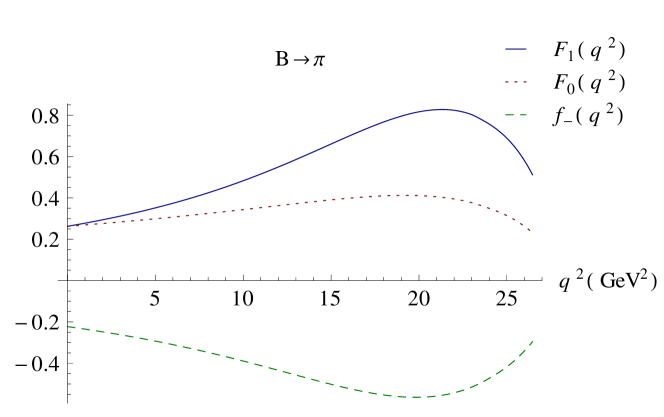
Figure 7.2: $B\to K$ and $B\to\pi$ transition form factors in the whole range $0\leq q^{2}\leq(M_{B}-M_{K(\pi)})^{2}$. Parameters for the quark masses and harmonic-oscillator wave functions are taken from Tables 6.1 and  7.1, respectively. For the meson masses the current values given by the Particle Data Group are taken [57].

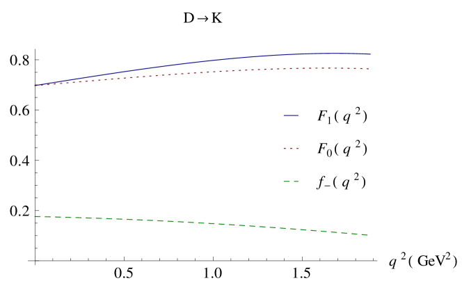
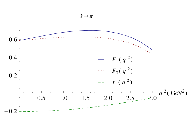
Figure 7.3: $D\to K$ and $D\to\pi$ transition form factors in the whole range $0\leq q^{2}\leq(M_{D}-M_{K(\pi)})^{2}$. Parameters for the quark masses and harmonic-oscillator wave functions are taken from Tables 6.1 and  7.1, respectively. For the meson masses the current values given by the Particle Data Group are taken [57].

7.3 Pseudoscalar-to-vector transitions

More interesting is the comparison for transitions that involve mesons with spin. In the light-front quark model [34], the form factors for pseudoscalar-to-vector meson transitions extracted in the $q_{\perp}=0$ frame, exhibit a certain frame dependence. For a given $q^{2}$, the form factors depend on whether the recoiling daughter moves in the positive “+” or negative “$-$” $z$-direction relative to the parent meson. In the light-front quark model the results for the form factors are larger in the “+” frame than in the “$-$” one. The exact vanishing of $Z$-graphs at $q^{2}=0$ in the “+” frame is taken as an argument in Ref. [34] to conclude that $Z$-graphs are less important in the “+” frame than in the “$-$” frame. In Table 7.7 results for both frames together with the point-form results obtained in this work are given at $q^{2}=0$. The authors of [34] interpret the difference between the results at $q^{2}=0$ in the “+” and “$-$” frames as a measure for the $Z$-graph contribution present in the “$-$” frame. In the point form, as explained in Chap. 3 and 4, all form factors can be extracted without ambiguity and no frame dependence appears in our description of weak decays. The current level of this work does not allow to give a serious estimate of $Z$-graph contributions. One could perhaps guess that they are of the same order of magnitude as the difference between “+” and “$-$” frames in front from.

In Tabs. 7.7-7.7 our from-factor results at $q^{2}=0$ are compared with those of Ref. [34] for several decays. One observes that the results obtained in the point form for $A_{0}(0)$, $A_{1}(0)$ and $A_{2}(0)$ are very similar in all the computed transitions, whereas they differ notably in the front form. There seems to be a good agreement between both approaches for $V(0)$ and $A_{0}(0)$. For these two form factors one sees that for the heavy-to-heavy transition the point-form result lies between the obtained ones in the front form in the “+” and “$-$” frames, being closer to the “+” one. $A_{1}(0)$ and $A_{2}(0)$ turn out to be larger in the point form in all cases.

For the whole $q^{2}$ range, i.e. $0\leq q^{2}\leq(M_{1}-M_{2})^{2}$, the form factors $V(q^{2})$, $A_{0}(q^{2})$, $A_{1}(q^{2})$ and $A_{2}(q^{2})$ are depicted in Figs. 7.4-7.8. If one compares with the corresponding plots in Ref. [34] the observations made already for $q^{2}=0$ are confirmed. For the $B$ decays our form factors resemble very much those of Ref. [34] (in the “+” frame) with $A_{2}(q^{2})$ showing the biggest deviations. For $D$-decays larger differences can be observed, in particular for $A_{1}(q^{2})$ and $A_{2}(q^{2})$, but the qualitative features of the form factors are still quite similar. This discrepancy is, of course, foreseeable since the point- and front-form approaches are not equivalent as long as one does not include non-valence contributions. The equivalence is only reached in the heavy-quark limit, where the same Isgur-Wise function is obtained.

$B\to D^{*}$	$V(0)$	$A_{0}(0)$	$A_{1}(0)$	$A_{2}(0)$
Front form [34] in the “+” frame	0.78	0.73	0.68	0.61
Front form [34] in the “$-$” frame	0.62	0.58	0.59	0.61
Point form (this work)	0.76	0.72	0.72	0.72

Table 7.3: Form factors at $q^{2}=0$ for the $B\to D^{*}$ transition obtained within the light-front quark model in Ref. [34] in the frames where the recoiling daughter moves in the positive $z$-direction (“+” frame) and negative $z$-direction (“$-$” frame) in comparison with the results obtained in the point form.

$B\to K^{*}$	$V(0)$	$A_{0}(0)$	$A_{1}(0)$	$A_{2}(0)$
Front form [34]	0.35	0.32	0.26	0.23
Point form [this work]	0.36	0.33	0.32	0.31

Table 7.4: Form factors at $q^{2}=0$ for the $B\to K^{*}$ transition obtained within the front-form quark model in the frame where where the recoiling daughter moves in the positive $z$-direction , i.e. “+” frame, and in the point form of relativistic quantum mechanics.

$D\to K^{*}$	$V(0)$	$A_{0}(0)$	$A_{1}(0)$	$A_{2}(0)$
Front form [34]	0.87	0.71	0.62	0.46
Point form [this work]	0.87	0.70	0.71	0.73

Table 7.5: Same comparison as in Table 7.7 but for the $B\to K^{*}$ transition.

$B\to\rho$	$V(0)$	$A_{0}(0)$	$A_{1}(0)$	$A_{2}(0)$
Front form [34]	0.30	0.28	0.20	0.18
Point form [this work]	0.31	0.28	0.27	0.26

Table 7.6: Same comparison as in Table 7.7 but for the $B\to\rho$ transition.

$D\to\rho$	$V(0)$	$A_{0}(0)$	$A_{1}(0)$	$A_{2}(0)$
Front form [34]	0.78	0.63	0.51	0.34
Point form [this work]	0.80	0.63	0.64	0.64

Table 7.7: Same comparison as in Table 7.7 but for the $D\to\rho$ transition.

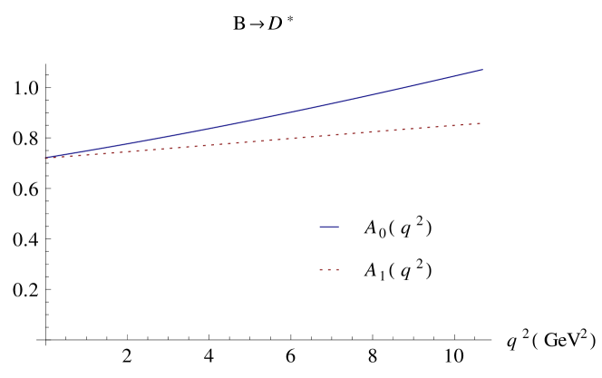
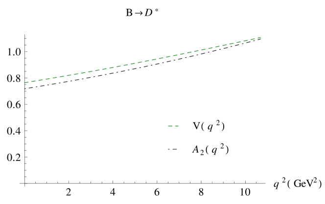
Figure 7.4: $B\to D^{*}$ transition form factors in the whole range $0\leq q^{2}\leq(M_{B}-M_{D^{*}})^{2}$. Parameters for the quark masses and harmonic-oscillator wave functions are taken from Tables 6.1 and 7.1 respectively. For the meson masses the current values given by the Particle Data Group are taken [57].

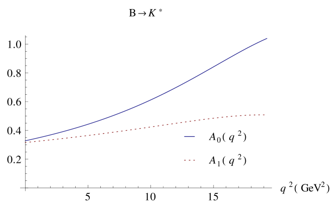
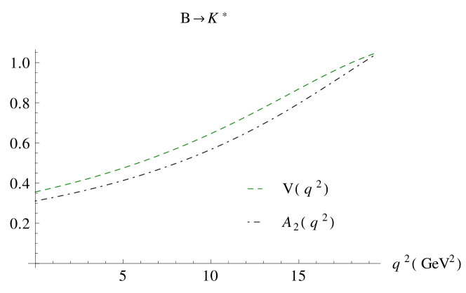
Figure 7.5: $B\to K^{*}$ transition form factors in the whole range $0\leq q^{2}\leq(M_{B}-M_{K^{*}})^{2}$. Parameters for the quark masses and harmonic-oscillator wave functions are taken from Tables 6.1 and 7.1 respectively. For the meson masses the current values given by the Particle Data Group are taken [57].

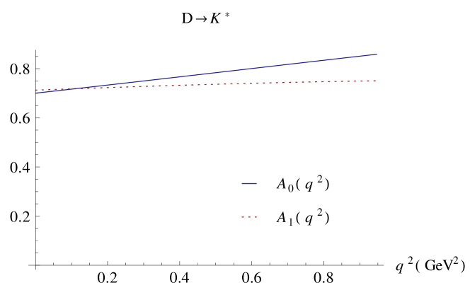
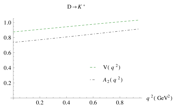
Figure 7.6: $D\to K^{*}$ transition form factors in the whole range $0\leq q^{2}\leq(M_{D}-M_{K^{*}})^{2}$. Parameters for the quark masses and harmonic-oscillator wave functions are taken from Tables 6.1 and 7.1 respectively. For the meson masses the current values given by the Particle Data Group are taken [57].

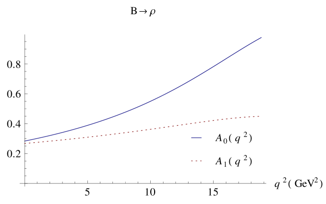
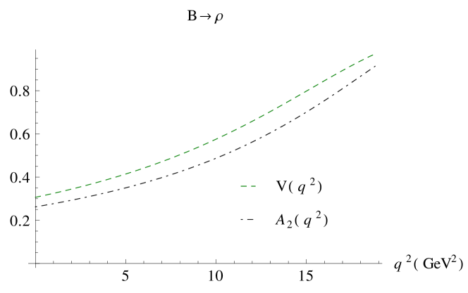
Figure 7.7: $B\to\rho$ transition form factors in the whole range $0\leq q^{2}\leq(M_{B}-M_{\rho})^{2}$. Parameters for the quark masses and harmonic-oscillator wave functions are taken from Tables 6.1 and 7.1 respectively. For the meson masses the current values given by the Particle Data Group are taken [57].

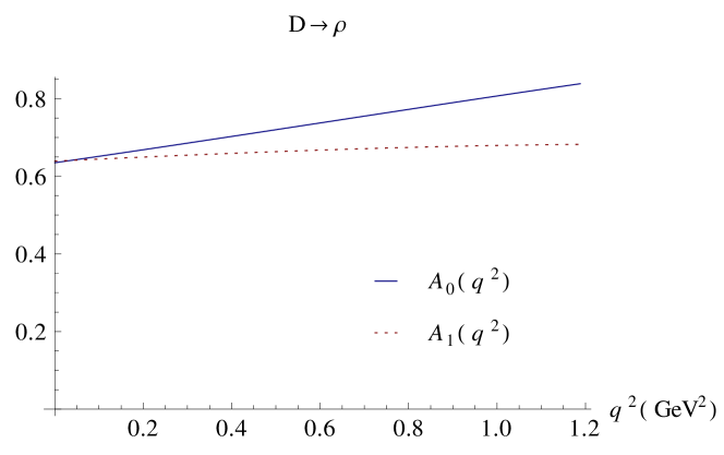
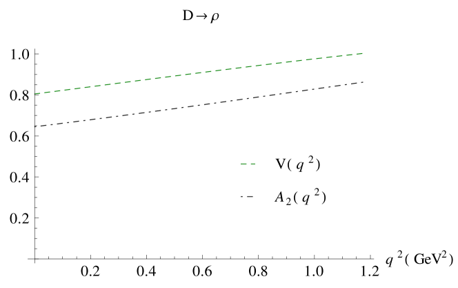
Figure 7.8: $D\to\rho$ transition form factors in the whole range $0\leq q^{2}\leq(M_{B}-M_{\rho})^{2}$. Parameters for the quark masses and harmonic-oscillator wave functions are taken from Tables 6.1 and 7.1 respectively. For the meson masses the current values given by the Particle Data Group are taken [57].

7.4 Conclusions and outlook

In this chapter numerical results for a simple harmonic-oscillator wave function with different harmonic-oscillator parameters for each meson have been presented in the range $0\leq q^{2}\leq(M_{1}-M_{2})^{2}$. Form factors are extracted without ambiguity for both, pseudoscalar-to-pseudoscalar and pseudoscalar-to-vector meson transitions.

The harmonic-oscillator wave function seems still to be too simple to do quantitative predictions that can be compared with experiments, but qualitative features of the point form approach can be studied numerically. To compare with, analogous calculation in the front-form approach have been considered. While in the front form the obtained results for pseudoscalar-to-vector transitions exhibits a certain dependence on the reference frame, i.e. on whether the recoiling daughter moves in the positive or negative $z$-direction relative to the parent meson, in the point form all form factors are determined unambiguously.

In the heavy-quark limit, as was shown in Chap. 6, point-form and front-form calculations yield the same numerical result for the Isgur-Wise function. This equivalence is possible because in the heavy-quark limit nonvalence contributions in the form of $Z$-graph vanish. For finite heavy-quark masses, the point form and the front form are not equivalent, since the role that the $Z$-graph contributions play in either approach differs. This is shown by the numerical results presented in this chapter. The non-valence contributions enter in a different way in the point and in the front forms.

As long as $Z$-graph contributions are not introduced, it will be not possible to give a full answer in the whole $q^{2}$-range. It will be the subject of future work to introduce non-valence contributions in the coupled channel approach and to investigate how they affect the form factors. Similar studies on this subject have been carried out already in the front form [37]. Like in Ref. [37] an estimate on $Z$-graph contributions within our approach could be obtained by calculating the transition form factors in the space-like region, where one can go into the infinite-momentum frame and continue those results analytically to the time-like momentum-transfer region. The difference with the present calculation should then give an estimate of the size of $Z$-graph contributions.

Chapter 8 Dynamical binding forces

8.1 Introduction

So far we have considered two-body states that are bound by instantaneous forces. In this chapter we will have a look at binding forces that are caused by dynamical particle exchange. Taking into account the retardation effects of the exchange particle requires the introduction of more channels in the mass eigenvalue problem. We will illustrate this with a simple example. We consider the deuteron as a system of two nucleons which interact via $\sigma$- and $\omega$-exchange, i.e. a Walecka type model [63]. This is part of a benchmark calculation initiated during a workshop at ECT* Trento in 2009 with the goal of comparing relativistic effects as resulting from different approaches using common parameters. The starting point was nonrelativistic quantum mechanics [21, 64] with the static approximation of $\sigma$- and $\omega$-exchange to compute the common parameters. This provided the first step for the investigation of relativistic effects in different approaches. Here we make a next step towards the understanding of the role that relativity plays in the description of electromagnetic properties of strongly bound states.

Dynamical meson exchange gives rise to relativistic corrections. These corrections will not only change the binding energy of the deuteron, they also modify the bound-state wave function and hence the electromagnetic properties of the deuteron as tested in electron-deuteron scattering. The photon exchanged between the electron and the deuteron can resolve the internal structure of the bound state. Its coupling to the nucleons may take place during the meson exchange and furthermore, if the exchanged mesons are charged, the photon can also couple to them. Such meson-exchange currents become important at momentum transfer squared of a few GeV². In order to account for these processes a consistent relativistic description for both, the bound-state wave function and for the electron-deuteron scattering amplitude, is necessary. In the following we will present an appropriate theoretical framework and we will give the numerical solution for the relativistic wave function as resulting from the dynamical boson-exchange responsible for the binding in the Walecka model.

8.2 The Walecka model

The interaction term of the Lagrangian density in the Walecka model is given by

$$\hat{\mathcal{L}}_{\text{int}}=g_{\sigma}\hat{\bar{\psi}}_{N}\hat{\psi}_{N}\hat{\sigma}+ig_{\omega}\hat{\bar{\psi}}_{N}\gamma_{\mu}\hat{\psi}_{N}\hat{\omega}^{\mu}+\frac{f_{\omega}}{4m_{N}}\hat{\bar{\psi}}_{N}\sigma_{\mu\nu}\hat{\psi}_{N}(\partial^{\mu}\hat{\omega}^{\nu}-\partial^{\nu}\hat{\omega}^{\mu}),$$ (8.1)

where $\hat{\psi}_{N}(x)$ is the nucleon field of mass $m_{N}$, $\hat{\sigma}(x)$ is a neutral scalar meson field of mass $m_{\sigma}$ and $\hat{\omega}(x)$ a neutral vector meson field of mass $m_{\omega}$. The $\sigma$-exchange is responsible for the binding of the nucleons, while the $\omega$ is associated to repulsive effects. The Walecka model requires regularization. We introduce Pauli-Villars particles [65] which we call $\sigma_{PV}$ and $\omega_{PV}$, with masses $\Lambda_{\sigma}$ and $\Lambda_{\omega}$, respectively. The Lagrangian density terms of this fields have identical form to the ones corresponding to the physical particles but are multiplied by a factor $i$.

The notation used in this chapter will be: capital $N$ for “nucleon” and lower-case $n$ and $p$ for “neutron” and “proton”, respectively. The parameters calculated in the static approximation [21, 64] will be used in the following. They are shown in Table 8.1.

Parameters	Biernat et al. [21, 64]	[21, 64] no PV
$E_{B}$ (MeV)	-2.224575	-3.36772
$a_{t}$ (fm)	5.4151	4.58658
$g^{2}_{\sigma}/4\pi$	6.31	6.31
$g^{2}_{\omega}/4\pi$	18.617	18.617
$m_{\sigma}$ (MeV/$c^{2}$)	400	400
$m_{\omega}$ (MeV/$c^{2}$)	782.7	782.7
$\Lambda_{\sigma}$ (MeV/$c^{2}$)	1000	$\infty$
$\Lambda_{\omega}$ (MeV/$c^{2}$)	1500	$\infty$

Table 8.1: Walecka model parameters considered for the numerical calculations of this chapter. Masses and coupling constants were chosen such that the deuteron binding energy $E_{B}$ and the scattering length $a_{t}$ are reproduced [21, 64]. In accordance with realistic models the tensor coupling of the $\omega$ is neglected, i.e. $f_{\omega}=0$.

The next step to understand the role of relativity in the description of two-body bound states requires to abandon the static approximation and to take the dynamics of the exchanged particles fully into account. For the sake of simplicity we will still consider the $\omega$-meson exchange, which provides the short-range repulsion, in the static limit; only the retardation of the $\sigma$-exchange, which is responsible for the binding, will be taken into account. The fact that in this model we consider only neutral mesons makes the problem much simpler since the photon cannot couple to them. We will study the relativistic effects that are due to the retardation of the $\sigma$-meson.

8.3 The deuteron bound-state problem

We present in this section the bound-state problem from which the deuteron wave function will be obtained. The deuteron wave function for our Walecka-type model was already computed numerically by Biernat [21, 64] using the point-form approach in the approximation where the $\sigma$- and $\omega$-exchanges were instantaneous [21, 64]. Let us first consider the generalization in which both, the $\sigma$- and the $\omega$-exchange, are treated dynamically. The mass-eigenvalue equation for the 2-nucleon system in this case can be formulated as the following coupled-channel problem:

$$\left(\begin{array}[]{ccc}\hat{M}_{np}&\hat{K}_{\sigma}&\hat{K}_{\omega}\\ \hat{K}^{\dagger}_{\sigma}&\hat{M}_{np\sigma}&0\\ \hat{K}^{\dagger}_{\omega}&0&\hat{M}_{np\omega}\end{array}\right)\left(\begin{array}[]{c}|\psi_{np}\rangle\\ |\psi_{np\sigma}\rangle\\ |\psi_{np\omega}\rangle\end{array}\right)=m\left(\begin{array}[]{c}|\psi_{np}\rangle\\ |\psi_{np\sigma}\rangle\\ |\psi_{np\omega}\rangle\end{array}\right).$$ (8.2)

The vanishing matrix elements impose the condition that no more than one meson can be exchanged simultaneously. Applying a Feshbach reduction one obtains the reduced eigenvalue equation for the 2-nucleon component we want to solve:

$$\hat{M}_{np}|\psi_{np}\rangle+\hat{K}_{\sigma}(m-\hat{M}_{np\sigma})^{-1}\hat{K}_{\sigma}^{\dagger}|\psi_{np}\rangle+\hat{K}_{\omega}(m-\hat{M}_{np\omega})^{-1}\hat{K}_{\omega}^{\dagger}|\psi_{np}\rangle=m|\psi_{np}\rangle.$$ (8.3)

For simplicity, we will allow retardation only for the $\sigma$-exchange and we will keep the static limit in the $\omega$-exchange. In the approximation where the $\omega$-exchange is instantaneous, Eq. (8.3) can be written as (see also Fig. 8.1):

$$\left(\hat{M}_{np}+\hat{V}_{\omega}^{\text{inst}}+\hat{K}_{\sigma}(m-\hat{M}_{np\sigma})^{-1}\hat{K}^{\dagger}_{\sigma}\right)|\psi_{np}\rangle=m|\psi_{np}\rangle.$$ (8.4)

The mass operators $\hat{M}_{np}$ and $\hat{M}_{np\sigma}$ account for the relativistic kinetic energies of the free particles, i.e.

$$\hat{M}_{np}|v;\vec{k}_{p},\mu_{p};\vec{k}_{n},\mu_{n}\rangle =\left(\omega_{k_{p}}+\omega_{k_{n}}\right)|v;\vec{k}_{p},\mu_{p};\vec{k}_{n},\mu_{n}\rangle,$$ (8.5)

$$\hat{M}_{np\sigma}|v;\vec{k}_{p},\mu_{p};\vec{k}_{n},\mu_{n};\vec{k}_{\sigma}\rangle =\left(\omega_{k_{p}}+\omega_{k_{n}}+\omega_{k_{\sigma}}\right)|v;\vec{k}_{p},\mu_{p};\vec{k}_{n},\mu_{n};\vec{k}_{\sigma}\rangle.$$ (8.6)

We are now interested in bound-state solutions of Eq. (8.4), which have the quantum numbers of the deuteron. $|\psi_{np}\rangle$ is thus a 1-particle velocity state with the (discrete) quantum numbers $\alpha_{D}$ of the deuteron, i.e. $|\psi_{np}\rangle=|\underline{v};\alpha_{D}\rangle$. Since neither the instantaneous $\omega$-exchange nor the scalar $\sigma$-exchange can couple $s$- and $d$-waves, our deuteron is still a pure $s$-wave bound state. This means that the matrix element $\langle\underline{v};\vec{k}_{p},\mu_{p};\vec{k}_{n},\mu_{n}|\psi_{np}\rangle$ can be written in the form:

$$\langle v;\vec{k}_{p},\mu_{p};\vec{k}_{n},\mu_{n}|\psi_{np}\rangle= (2\pi)^{9/2}\underline{v}_{0}\delta^{3}(\vec{\underline{v}}-\vec{v})\sqrt{\frac{2}{m_{D}}}\sqrt{\frac{2\omega_{k_{n}}2\omega_{k_{p}}}{(\omega_{k_{n}}+\omega_{k_{p}})^{3}}}$$

$$\times C^{1\mu_{D}}_{\frac{1}{2}\mu_{n}\frac{1}{2}\mu_{p}}\text{u}_{D}(|\vec{k}_{p}|)\text{Y}_{00}(\hat{k}_{p}).$$ (8.7)

Multiplying Eq. (8.4) by $\langle\underline{v};\vec{k}_{p},\mu_{p};\vec{k}_{n},\mu_{n}|$ and using this relation one obtains the integral equation for the deuteron wave function:

$$\left(\omega_{k_{p}}+\omega_{k_{n}}\right)\tilde{\text{u}}_{D}(|\vec{k}|)+\int\frac{d^{3}k^{\prime}}{(2\pi)^{3}}\left(\tilde{v}_{\text{int}}^{N\omega}(\vec{k},\vec{k}^{\prime})+\tilde{v}_{\text{int}}^{N\sigma}(\vec{k},\vec{k}^{\prime})\right)\tilde{\text{u}}_{D}(|\vec{k}^{\prime}|)=m_{D}\tilde{\text{u}}_{D}(|\vec{k}|)$$ (8.8)

with

$$\tilde{v}_{\text{int}}^{N\omega}(\vec{k},\vec{k}^{\prime})=\;\frac{g_{\omega}^{2}}{(\vec{k}-\vec{k}^{\prime})^{2}+m^{2}_{\omega}}-\frac{g_{\omega}^{2}}{(\vec{k}-\vec{k}^{\prime})^{2}+\Lambda^{2}_{\omega}},$$ (8.9)

$$\tilde{v}_{\text{int}}^{N\sigma}(\vec{k},\vec{k}^{\prime})=\left(\frac{\omega_{k^{\prime}_{p}}}{\omega_{k_{p}}}\right)^{3/2}\sum_{\mu_{p}^{\prime}\mu_{n}^{\prime}}\frac{\bar{u}_{\mu_{n}}(\vec{k}_{n})u_{\mu^{\prime}_{n}}(\vec{k}_{n}^{\prime})}{2\omega_{k^{\prime}_{n}}}\frac{\bar{u}_{\mu_{p}}(\vec{k}_{p})u_{\mu^{\prime}_{p}}(\vec{k}_{p}^{\prime})}{2\omega_{k^{\prime}_{p}}}$$

$$\;\;\times\left(\frac{g_{\sigma}^{2}}{\omega_{k_{\sigma}}(m_{D}-\omega_{k_{p}}-\omega_{k^{\prime}_{p}}-\omega_{k_{\sigma}})}-\frac{g_{\sigma}^{2}}{\omega_{k_{\sigma PV}}(m_{D}-\omega_{k_{p}}-\omega_{k^{\prime}_{p}}-\omega_{k_{\sigma PV}})}\right).$$ (8.10)

where the notation $\tilde{\text{u}}_{D}(|\vec{k}^{(\prime)}|):=(\omega_{k_{p}^{(\prime)}})^{-1/2}\text{u}_{D}(|\vec{k}^{(\prime)}|)$ and $\vec{k}:=\vec{k}_{p}=-\vec{k}_{n}$, has been used. Note that now the kernel depends on the eigenvalue $m_{D}$.

The problem can be solved numerically using Gaussian quadrature, following analogous steps as in Refs. [21, 66, 64]. The wave-function solution of the integral equation will be used for the calculation of transition amplitudes and currents analogously to Chaps. 3 and 4. $\text{u}_{D}(|\vec{k}|)$ has to be appropriately normalized such that

$$\langle\psi_{np}|\psi_{np}\rangle+\langle\psi_{np\sigma}|\psi_{np\sigma}\rangle=(2\pi)^{3}\frac{2}{m^{2}_{D}}v^{0}\delta^{3}(\vec{v}^{\prime}-\vec{v}),$$ (8.11)

where $\vec{v}^{\prime}$ is the velocity of the bra and $\vec{v}$ the one of the ket. To compute $|\psi_{np\sigma}\rangle$, one can use:

$$|\psi_{np\sigma}\rangle=\left(m_{D}-M_{np\sigma}\right)^{-1}\hat{K}^{\dagger}|\psi_{np}\rangle,$$ (8.12)

which follows from Eq. (8.2). Hence the matrix element$\langle v;\vec{k}_{p},\mu_{p};\vec{k}_{n},\mu_{n};$ $\vec{k}_{\sigma}|\psi_{np\sigma}\rangle$ can be expressed in terms of the deuteron wave function $\text{u}_{D}(|\vec{k}_{p}|)$. The analytical expression is given in App. D.1.1.

Figure 8.1: Graphical representation of the one-boson exchange kernel occurring in the deuteron bound-state problem (cf. Eq. (8.4)). There is a repulsive core described by an instantaneous $\omega$-exchange. The attraction is provided by $\sigma$-exchange. The $\sigma$-dynamics is fully taken into account.

8.4 The electron-deuteron scattering problem

The bound-state wave function obtained in this manner will be used in the coupled-channel problem that describes electron-deuteron scattering. The corresponding mass-eigenvalue problem needs 4-channels:

$$\left(\begin{array}[]{cccc}\hat{M}_{enp}+\hat{V}_{\omega}^{\text{inst}}&\hat{K}_{\gamma}&\hat{K}_{\sigma}&0\\ \hat{K}_{\gamma}^{\dagger}&\hat{M}_{enp\gamma}+\hat{V}_{\omega}^{\text{inst}}&0&\hat{K}_{\sigma}\\ \hat{K}_{\sigma}^{\dagger}&0&\hat{M}_{enp\sigma}&\hat{K}_{\gamma}\\ 0&\hat{K}_{\sigma}^{\dagger}&\hat{K}_{\gamma}^{\dagger}&\hat{M}_{enp\gamma\sigma}\end{array}\right)\left(\begin{array}[]{c}|\psi_{enp}\rangle\\ |\psi_{enp\gamma}\rangle\\ |\psi_{enp\sigma}\rangle\\ |\psi_{enp\gamma\sigma}\rangle\end{array}\right)=m\left(\begin{array}[]{c}|\psi_{enp}\rangle\\ |\psi_{enp\gamma}\rangle\\ |\psi_{enp\sigma}\rangle\\ |\psi_{enp\gamma\sigma}\rangle\end{array}\right).$$ (8.13)

The diagonal part represents the kinetic energy of the free particles plus instantaneous forces. Here the eigenvalue is $m=\omega_{e}+\omega_{D}$. In analogy to the electron-meson scattering problem, the system of equations can be reduced to a single equation for the $|\psi_{enp}\rangle$ state

$$\{\hat{M}_{eD}+$$

$$+ \hat{K}_{\gamma}(m-\hat{M}_{eD\gamma})^{-1}\hat{K}^{\dagger}_{\gamma}$$

$$+ \hat{K}_{\gamma}(m-\hat{M}_{eD\gamma})^{-1}\hat{K}_{\sigma}(m-\hat{M}_{enp\sigma\gamma})^{-1}\hat{K}^{\dagger}_{\gamma}(m-\hat{M}_{enp\sigma})^{-1}\hat{K}_{\sigma}^{\dagger}$$

$$+ \hat{K}_{\sigma}(m-\hat{M}_{enp\sigma})^{-1}\hat{K}_{\gamma}(m-\hat{M}_{enp\sigma\gamma})^{-1}\hat{K}_{\gamma}^{\dagger}(m-\hat{M}_{enp\sigma})^{-1}\hat{K}_{\sigma}^{\dagger}$$

$$+ \hat{K}_{\sigma}(m-\hat{M}_{enp\sigma})^{-1}\hat{K}_{\gamma}(m-\hat{M}_{enp\sigma\gamma})^{-1}\hat{K}_{\sigma}^{\dagger}(m-\hat{M}_{eD\gamma})^{-1}\hat{K}_{\gamma}^{\dagger}$$

$$+ \hat{K}_{\sigma}(m-\hat{M}_{enp\sigma})^{-1}\hat{K}_{\gamma}(m-\hat{M}_{enp\sigma\gamma})^{-1}\hat{K}_{\sigma}^{\dagger}(m-\hat{M}_{eD\gamma})^{-1}$$

$$\times\hat{K}_{\sigma}(m-\hat{M}_{enp\sigma\gamma})^{-1}\hat{K}_{\gamma}^{\dagger}(m-\hat{M}_{enp\sigma})^{-1}\hat{K}_{\sigma}^{\dagger}\}|\Psi_{enp}\rangle=m|\Psi_{enp}\rangle,$$

where the following notation has been used:

$$\hat{M}_{eD}:=\hat{M}_{enp}+\hat{V}^{\text{inst}}_{\omega}+\hat{K}_{\sigma}(m-\hat{M}_{enp\sigma})^{-1}\hat{K}^{\dagger}_{\sigma}.$$ (8.15)

Now $\hat{M}_{eD}$ and $\hat{M}_{eD\gamma}$ have eigenstates

$$\hat{M}_{eD}\,|\underline{v};\underline{\vec{k}}_{e},\underline{\mu}_{e};\underline{\vec{k}}_{D},\underline{\mu}_{D}\rangle =(\omega_{k_{e}}+\omega_{k_{D}})\,|\underline{v};\underline{\vec{k}}_{e},\underline{\mu}_{e};\underline{\vec{k}}_{D},\underline{\mu}_{D}\rangle,$$ (8.16)

$$\hat{M}_{eD\gamma}\,|\underline{v};\underline{\vec{k}}_{e},\underline{\mu}_{e};\underline{\vec{k}}_{D},\underline{\mu}_{D};\underline{\vec{k}}_{\gamma},\underline{\mu}_{\gamma}\rangle =(\omega_{k_{e}}+\omega_{k_{D}}+\omega_{k_{\gamma}})\,|\underline{v};\underline{\vec{k}}_{e},\underline{\mu}_{e};\underline{\vec{k}}_{D},\underline{\mu}_{D};\underline{\vec{k}}_{\gamma},\underline{\mu}_{\gamma}\rangle.$$ (8.17)

with $\omega_{k_{D}}=\sqrt{m_{D}^{2}+\vec{k}_{D}^{2}}$, $\omega_{k_{e}}=\sqrt{m_{e}^{2}+\vec{k}_{e}^{2}}$, and $\omega_{k_{\gamma}}=|\vec{k}_{\gamma}|$.

Eq. (8.4) describes the electron-deuteron scattering process in analogy to what was done for two-body systems that are bound by instantaneous confining forces. Now, however, the binding is generated by the dynamical $\sigma$-exchange, which leads to additional terms in the 1-photon-exchange optical potential. In the following we will discuss those terms. By the replacement (8.15) one absorbs the sigma exchange into the deuteron wave function.

8.4.1 Graphical representation

One-body currents

The first term in Eq. (8.4) represents the kinetic energy of the electron-deuteron system, with the deuteron binding being determined by dynamical $\sigma$-exchange and an instantaneous $\omega$-exchange. The other terms in Eq. (8.4) represent the 1-photon-exchange potential and thus determine the electromagnetic deuteron current. For instance, the second term

$$\hat{K}_{\gamma}(m-\hat{M}_{eD\gamma})^{-1}\hat{K}^{\dagger}_{\gamma}$$ (8.18)

has the same form as the optical potential in Eq. (3.10) for the case of systems which are bound by an instantaneous potential. It gives rise to the four time-ordered contributions that are sketched in Fig. 8.2. The gray ovals represent the deuteron. Already these graphs contain ralativistic corrections which go beyond instantaneous binding forces, namely the retardation effect of the $\sigma$ in the deuteron wave function. As in Sec. 3 the electromagnetic deuteron current extracted from these graphs is a one-body current.

Exchange currents

In the following we discuss those contributions to electron-deuteron scattering which give rise to the, so-called, exchange currents. These are the terms in the optical potential that describe the coupling of the photon to the nucleons during the $\sigma$-meson exchange. Figures 8.3 and 8.4 are graphical representations of (part of) the photon and $\sigma$-exchanges described by the third and fifth terms in Eq. (8.4). Initially, a $\sigma$-meson is emitted by one of the nucleons, the $enp\sigma$-system propagates freely until a photon is emitted by one of the nucleons; then the $enp\sigma\gamma$-system propagates freely until the $\sigma$-meson is absorbed by the second nucleon. Finally, the deuteron-bound state propagates together with the photon and the electron, until the photon is absorbed by the electron. The fourth term (see Fig. 8.5) represents the case in which the whole $\gamma$-exchange (emission and absorption) occurs during the $\sigma$-exchange process.

A representative example of a one-photon-exchange graph corresponding to the sixth term is given in Fig. 8.6. The significance of this type of graphs is still not clear to us. They could be necessary to get the correct normalization of the deuteron form factors at the end. Therefore we will concentrate on the graphs shown in Figs. 8.2-8.4.

Electromagnetic self-energy graphs in which the photon is emitted and absorbed by the same particle (electron or nucleon) are also contained in Eq. (8.4). But they are not of interest here, because they do not contribute to photon-exchange between the electron and the deuteron. More interesting, however, are those graphs in which the $\sigma$ is emitted and reabsorbed by the same nucleon while the photon couples to the nucleon. There are also contained in Eq. (8.4) and represent strong vertex correction to the photon-nucleon vertex. Such corrections, however, should, at least partly, be contained in the electromagnetic nucleon form factors. We therefore omit them here too.

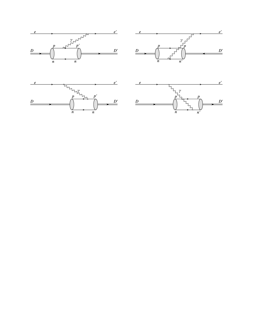
Figure 8.2: Graphical representation of the one photon exchange in electron-deuteron scattering corresponding to the term (8.18) of the optical potential. The sketch represents the four possible time orderings of this particular contribution, where the photon-nucleon coupling occurs during the time in which no $\sigma$-meson exchange takes place. The bound state, however, represented by the gray oval, accounts for the dynamical exchange given by the $\sigma$-potential, as well as for the instantaneous one corresponding to the $\omega$.

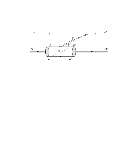
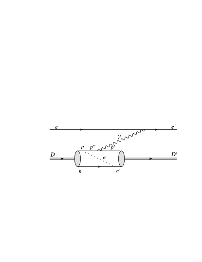
Figure 8.3: Graphical representation of the one-photon exchange in electron-deuteron scattering corresponding to the term $\hat{K}_{\gamma}(m-\hat{M}_{eD\gamma})^{-1}\hat{K}_{\sigma}(m-\hat{M}_{enp\sigma\gamma})^{-1}\hat{K}^{\dagger}_{\gamma}(m-\hat{M}_{enp\sigma})^{-1}\hat{K}_{\sigma}^{\dagger}$ in the optical potential (8.4). Graphs in which the photon couples to the neutron are not shown.

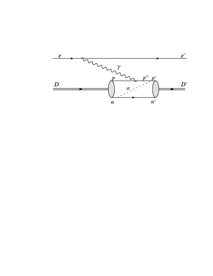
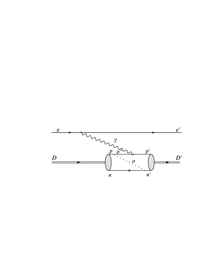
Figure 8.4: Graphical representation of the one-photon exchange in electron-deuteron scattering corresponding to the term $\hat{K}_{\sigma}(m-\hat{M}_{enp\sigma})^{-1}\hat{K}_{\gamma}(m-\hat{M}_{enp\sigma\gamma})^{-1}\hat{K}_{\sigma}^{\dagger}(m-\hat{M}_{eD\gamma})^{-1}\hat{K}_{\gamma}^{\dagger}$ in the optical potential (8.4). Graphs in which the photon couples to the neutron are not shown.

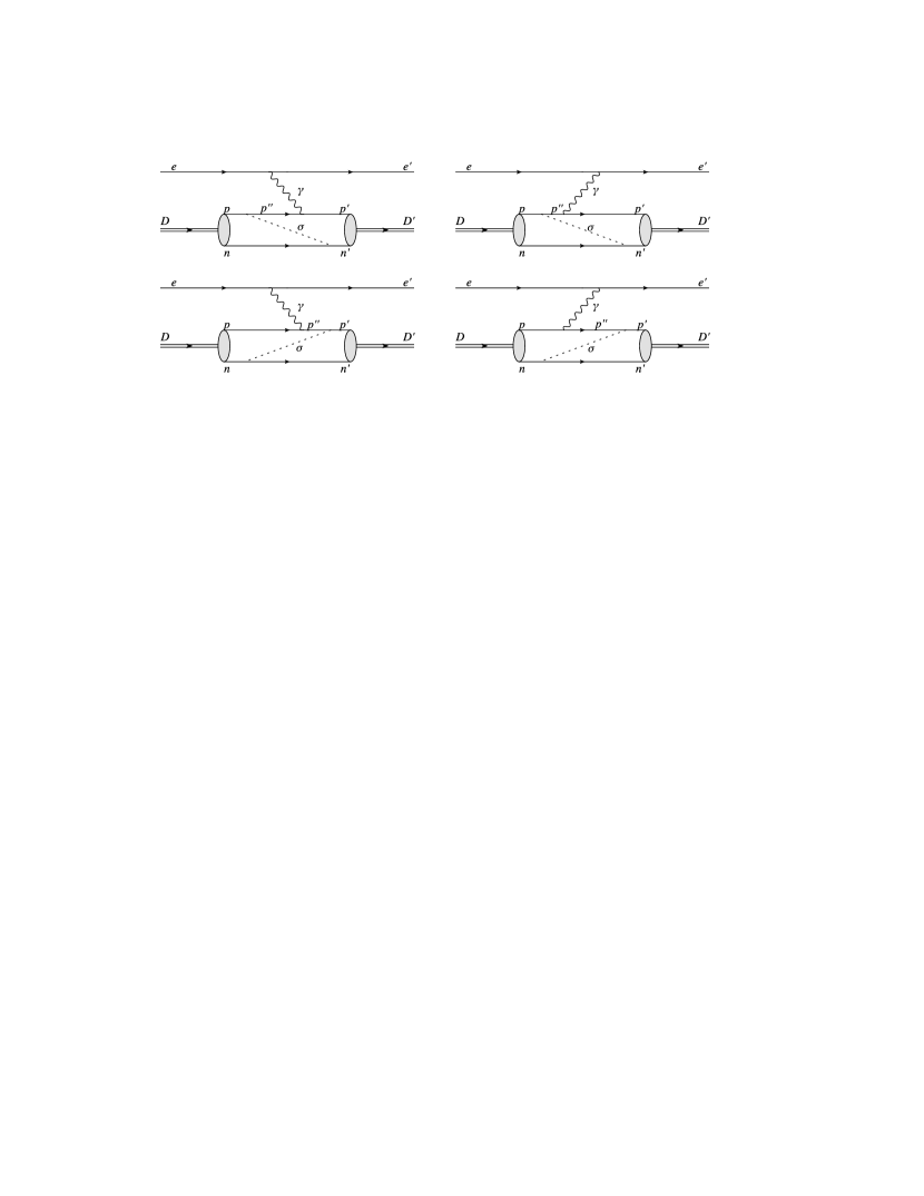
Figure 8.5: Graphical representation of the one-photon exchange in electron-deuteron scattering corresponding to the term $\hat{K}_{\sigma}(m-\hat{M}_{enp\sigma})^{-1}\hat{K}_{\gamma}(m-\hat{M}_{enp\sigma\gamma})^{-1}\hat{K}_{\gamma}^{\dagger}(m-\hat{M}_{enp\sigma})^{-1}\hat{K}_{\sigma}^{\dagger}$ in the optical potential (8.4). Graphs in which the photon couples to the neutron are not shown.

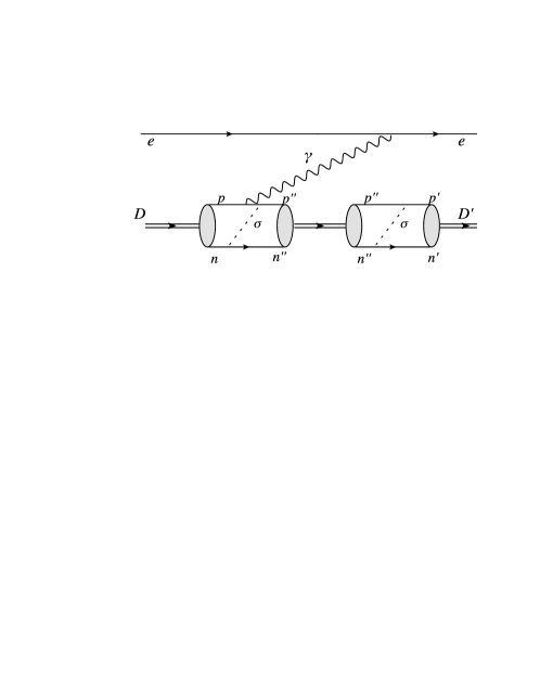
Figure 8.6: Graphical representation of the one-photon exchange in electron-deuteron scattering corresponding to the term $\hat{K}_{\sigma}(m-\hat{M}_{enp\sigma})^{-1}\hat{K}_{\gamma}(m-\hat{M}_{enp\sigma\gamma})^{-1}\hat{K}_{\sigma}^{\dagger}(m-\hat{M}_{eD\gamma})^{-1}\hat{K}_{\sigma}(m-\hat{M}_{enp\sigma\gamma})^{-1}\hat{K}_{\gamma}^{\dagger}(m-\hat{M}_{enp\sigma})^{-1}\hat{K}_{\sigma}^{\dagger}$ in the optical potential (8.4). Graphs in which the photon couples to the neutron and in which the time orderings of the $\gamma$- and $\sigma$-exchanges are reversed are not shown.

8.4.2 Currents and form factors

In this section we present the analytical expression for the electromagnetic currents as extracted from the one-photon-exchange optical potential in Eq. (8.4) (see also Figs. 8.2-8.6). Two kinds of contributions to the current can be distinguished from the discussion presented above, namely the one corresponding to one-body currents, i.e. those contributions where the exchanged $\sigma$ is in the deuteron wave function, and those in which $\sigma$-exchange happens at the same time as the photon exchange; these are called exchange currents. Some remarks on the covariance and cluster separability properties of these currents and form factors will be discussed.

One-body currents

The transition amplitude is computed exactly in the same way as it was done for the case of mesons (cf. Chap. 3):

$$\langle\underline{v^{\prime}};\vec{\underline{k}}^{\prime}_{e},\underline{\mu}^{\prime}_{e};\vec{\underline{k}}^{\prime}_{D},\underline{\mu}^{\prime}_{D}|\hat{K}_{\gamma}(m-\hat{M}_{eD\gamma})^{-1}\hat{K}^{\dagger}_{\gamma}|\underline{v};\vec{\underline{k}}_{e},\underline{\mu}_{e};\vec{\underline{k}}_{D},\underline{\mu}_{D}\rangle$$

$$\qquad=\underline{v}_{0}\delta(\vec{\underline{v}}^{\prime}-\vec{\underline{v}})\frac{(2\pi)^{3}}{\sqrt{(\omega_{k^{\prime}_{e}}+\omega_{\underline{k}^{\prime}_{D}})^{3}(\omega_{k_{e}}+\omega_{\underline{k}_{D}})^{3}}}$$

$$\qquad\qquad\times e\;\underbrace{\bar{u}_{\mu_{e}^{\prime}}(\vec{k}_{e}^{\prime})\gamma^{\mu}u_{\mu_{e}}(\vec{k}_{e})}_{j_{e}^{\mu}}\frac{(-g_{\mu\nu})}{\text{Q}^{2}}|e|\underbrace{(J_{p}^{\nu}+J_{n}^{\nu})}_{J_{D}^{\nu}},$$ (8.19)

with the proton current

$$J^{\nu}_{p}(\vec{k}^{\prime}_{D},\mu^{\prime}_{D};\vec{k}_{D},\mu_{D})=\sqrt{\omega_{\underline{k}^{\prime}_{D}}\omega_{\underline{k}_{D}}}\int\frac{d^{3}\tilde{k}_{p}^{\prime}}{\omega_{k_{p}}}\sqrt{\frac{\omega_{k_{p}}}{\omega_{k_{p}^{\prime}}}}\sqrt{\frac{m_{np}}{m_{np}^{\prime}}}$$

$$\quad\times\sum_{\mu_{p}^{\prime}\mu_{n}\mu_{p}}\sum_{\tilde{\mu}_{n}\tilde{\mu}_{p}\tilde{\mu}_{n}^{\prime}\tilde{\mu}_{p}^{\prime}}\bar{u}_{\mu_{p}^{\prime}}(\vec{k}_{p}^{\prime})\Gamma^{\nu}_{p}u_{\mu_{p}}(\vec{k}_{p})\;\text{u}^{*}_{D}(|\vec{\tilde{k}}_{p}^{\prime}|)Y^{*}_{00}(\hat{\vec{\tilde{k}}}_{p}^{\prime})\text{u}_{D}(|\vec{\tilde{k}}_{p}|)Y_{00}(\hat{\vec{\tilde{k}}}_{p})$$

$$\quad\times C^{1\mu_{D}^{\prime}}_{\frac{1}{2}\tilde{\mu}_{p}^{\prime}\frac{1}{2}\tilde{\mu}_{n}^{\prime}}\;D^{1/2}_{\tilde{\mu}_{p}^{\prime}\mu_{p}^{\prime}}\left[R_{W}^{-1}\left(\frac{\tilde{k}_{p}^{\prime}}{m_{p}},B_{c}\left(v_{np}\right)\right)\right]D^{1/2}_{\mu_{p}\tilde{\mu}_{p}}\left[R_{W}\left(\frac{\tilde{k}_{p}}{m_{p}},B_{c}\left(v_{np}\right)\right)\right]$$

$$\quad\times C^{1\mu_{D}}_{\frac{1}{2}\tilde{\mu}_{p}\frac{1}{2}\tilde{\mu}_{n}}D^{1/2}_{\tilde{\mu}_{n}^{\prime}\tilde{\mu}_{n}}\left[R_{W}^{-1}\left(\frac{\tilde{k}_{n}^{\prime}}{m_{n}},B_{c}\left(v_{np}^{\prime}\right)\right)R_{W}\left(\frac{\tilde{k}_{n}}{m_{n}},B_{c}\left(v_{np}\right)\right)\right].$$

An analogous expression is obtained for the neutron current. The $\Gamma^{\mu}_{N}$ in the nucleon current contains the nucleon structure:

$$\Gamma^{\mu}_{N}:=\left(F_{1N}(\text{Q}^{2})\gamma^{\mu}+F_{2N}(\text{Q}^{2})\frac{iq_{\nu}\sigma^{\nu\mu}}{2m_{N}}\right),\quad N=n,p.$$ (8.21)

where $F_{1N}(\text{Q}^{2})$ and $F_{2N}(\text{Q}^{2})$ are the electromagnetic form factors of the active nucleon, either the proton or the neutron, and $q^{\mu}=(k_{N}^{\prime\mu}-k_{N}^{\mu})$, $\sigma^{\mu\nu}=\frac{i}{2}(\gamma^{\mu}\gamma^{\nu}-\gamma^{\nu}\gamma^{\mu})$. For the calculations presented here we will later on consider the nucleons as point-like particles, using $F_{1p}(\text{Q}^{2})=1$ and $F_{2p}(\text{Q}^{2})=0$ for the proton, and $F_{1n}(\text{Q}^{2})=F_{2n}(\text{Q}^{2})=0$ for the neutron. This is $\Gamma^{\mu}\to\gamma^{\mu}$ and the photon coupling to the neutron vanishes.

Exchange currents

There are several terms in the potential (8.4) that contribute to the exchange currents we want to analyze in this chapter. They correspond to the case in which the photon couples to one of the nucleons while the process of $\sigma$-exchange, that keeps the system bound, takes place. The interaction between the nucleons should show up in the structure of the system, affecting therefore the form factors. The photon feels not only the interaction of the particle to which it couples since it is transfered to a system of three particles, one of them providing the binding interaction. We will present here first the analytical result for the exchange current corresponding to the third term in Eq. (8.4). It yields four graphs, two of them are illustrated in Fig. 8.3. We will explain the way how to extract the rest of them, which is straightforward with the correct interpretation of the diagrams shown in the previous section. Matrix elements of this term of the optical potential have the same structure as Eq. (8.4.2), but now the constituent current is much more complicated. One contribution that comes out from the third term in Eq. (8.4), namely the one corresponding to the left panel in Fig. 8.3 reads

$$J_{p}^{\mu,\text{ex}}(\vec{k}_{D}^{\prime},\vec{k}_{D};\mu^{\prime}_{D},\mu_{D})=\sqrt{2\omega_{k_{D}}2\omega_{k^{\prime}_{D}}}\int d^{3}\tilde{k}^{\prime}_{p}\int\frac{d^{3}\tilde{q}}{2\omega_{k_{\sigma}}}\sqrt{\frac{m_{np}}{m^{\prime}_{np}}}\sqrt{\frac{\omega_{k_{n}}}{\omega_{k^{\prime}_{n}}}}$$

$$\quad\times\left(\frac{1}{m-\omega_{k_{e}}-\omega_{k^{\prime\prime}_{p}}-\omega_{k^{\prime}_{n}}-\omega_{k_{\sigma}}-\omega_{k_{\gamma}}}\right)\left(\frac{1}{m-\omega_{k_{e}}-\omega_{k_{p}}-\omega_{k^{\prime}_{n}}-\omega_{k_{\sigma}}}\right)$$

$$\quad\times\sum_{\mu_{p}^{\prime}\mu_{n}\mu_{p}}\sum_{\tilde{\mu}_{n}\tilde{\mu}_{p}\tilde{\mu}_{n}^{\prime}\tilde{\mu}_{p}^{\prime}}\frac{\bar{u}_{\mu^{\prime}_{p}}(\vec{k}^{\prime\prime}_{p})\Gamma^{\nu}u_{\mu_{p}}(\vec{k}_{p})}{2\omega_{k_{p}}}\;g^{2}_{\sigma}\;\frac{\bar{u}_{\mu^{\prime}_{p}}(\vec{k}^{\prime}_{p})u_{\mu^{\prime}_{p}}(\vec{k}^{\prime\prime}_{p})}{2\omega_{k^{\prime\prime}_{p}}}\;\frac{\bar{u}_{\mu_{n}}(\vec{k}^{\prime}_{n})u_{\mu_{n}}(\vec{k}_{n})}{2\omega_{k_{n}}}$$

$$\quad\times C^{1\mu_{D}^{\prime}}_{\frac{1}{2}\tilde{\mu}_{p}^{\prime}\frac{1}{2}\tilde{\mu}_{n}^{\prime}}\;D^{1/2}_{\tilde{\mu}_{p}^{\prime}\mu_{p}^{\prime}}\left[R_{W}^{-1}\left(\frac{\tilde{k}_{p}^{\prime}}{m_{p}},B_{c}\left(v_{np}\right)\right)\right]D^{1/2}_{\mu_{p}\tilde{\mu}_{p}}\left[R_{W}\left(\frac{\tilde{k}_{p}}{m_{p}},B_{c}\left(v_{np}\right)\right)\right]$$

$$\quad\times C^{1\mu_{D}}_{\frac{1}{2}\tilde{\mu}_{p}\frac{1}{2}\tilde{\mu}_{n}}D^{1/2}_{\tilde{\mu}_{n}^{\prime}\tilde{\mu}_{n}}\left[R_{W}^{-1}\left(\frac{\tilde{k}_{n}^{\prime}}{m_{n}},B_{c}\left(v_{np}^{\prime}\right)\right)R_{W}\left(\frac{\tilde{k}_{n}}{m_{n}},B_{c}\left(v_{np}\right)\right)\right]$$

$$\quad\times\text{u}^{*}_{D}(|\vec{\tilde{k}}_{p}^{\prime}|)Y^{*}_{00}(\hat{\vec{\tilde{k}}}_{p}^{\prime})\text{u}_{D}(|\vec{\tilde{k}}_{p}|)Y_{00}(\hat{\vec{\tilde{k}}}_{p}),$$ (8.22)

where $\vec{\tilde{q}}$ is defined as $\vec{\tilde{q}}:=\vec{k}_{p}-\vec{k}_{p}^{\prime}$ (see App. D.2.1). Interchanging primed and unprimed variables one obtains the terms corresponding to the right panel of Fig. 8.4. The right graph in Fig. 8.3 is is identical to the left one except for the propagators. It is directly obtained by applying the changes

$$(m-\omega_{k_{e}}-\omega_{k^{\prime\prime}_{p}}-\omega_{k^{\prime}_{n}}-\omega_{k_{\sigma}}-\omega_{k_{\gamma}})^{-1}(m-\omega_{k_{e}}-\omega_{k_{p}}-\omega_{k^{\prime}_{n}}-\omega_{k_{\sigma}})^{-1}$$

$$\to(m-\omega_{k_{e}}-\omega_{k^{\prime}_{p}}-\omega_{k_{n}}-\omega_{k_{\sigma}}-\omega_{k_{\gamma}})^{-1}(m-\omega_{k_{e}}-\omega_{k_{p}^{\prime\prime}}-\omega_{k_{n}}-\omega_{k_{\sigma}})^{-1}$$

and

$$\bar{u}_{\mu^{\prime}_{p}}(\vec{k}^{\prime\prime}_{p})\Gamma^{\nu}u_{\mu_{p}}(\vec{k}_{p}) \to \bar{u}_{\mu_{p}^{\prime}}(\vec{k}^{\prime}_{p})\Gamma^{\nu}u_{\mu_{p}}(\vec{k}_{p}^{\prime\prime}),$$ (8.24)

$$\bar{u}_{\mu^{\prime}_{p}}(\vec{k}^{\prime}_{p})u_{\mu^{\prime}_{p}}(\vec{k}^{\prime\prime}_{p}) \to \bar{u}_{\mu_{p}}(\vec{k}^{\prime\prime}_{p})u_{\mu_{p}}(\vec{k}_{p}).$$ (8.25)

From the obtained result, by interchanging primed and unprimed variables one obtains the left graph in Fig. 8.4.

In addition to the integration over $\vec{\tilde{k}}^{\prime}_{p}$, a second integral appears, which runs over the intermediate state $\vec{\tilde{k}}^{\prime\prime}_{p}$, and accounts for the fact that momentum is transfered by the $\sigma$-meson from one nucleon to the other. By a change of variables one can go over to an integration over the momentum transfer, which we call $\vec{\tilde{q}}$. The change requires some work, because $\vec{\tilde{k}}^{\prime\prime}_{p}$ and $\vec{\tilde{q}}$ are defined in different reference frames. One has to transform $\vec{\tilde{k}}_{p}^{\prime\prime}$ to $\vec{k}_{p}^{\prime\prime}$ (see Eq. B.4), which is related to $\vec{\tilde{q}}$ by a simple translation.

It is not possible to combine all contributions in one term in a simple way as it was done for one-body currents. However, we will see that this will not be a problem for our purpose, since in the infinite-momentum frame, where the extraction of the form factors will be carried out (cf. Chap. 4), the binding energy becomes negligible and every propagator reduces to the same form, allowing to write the exchange currents as a one-term expression. We will see this in the following section.

8.4.3 Properties of the currents

The description of our electromagnetic spin-1 current requires 11 covariants and form factors (cf. Sec. 4.1.2). It is convenient to take the infinite momentum frame, i.e. $s\to\infty$, in order to get rid of most of the spurious contributions and to be able to determine the form factors from those matrix elements of the current that contain only physical contributions. The introduction of the $\sigma$-exchange does not alter the structure of the covariant decomposition. It modifies instead the microscopic structure of the current. The inclusion of these additional degrees of freedom might reduce, however, the strength of the non-physical quantities. In order to check this, a numerical study of the exchange currents and form factors is needed. In this work we will provide the analytical prerequisites. In the following, we present analytical results for the exchange current as resulting in the infinite-momentum frame. To do this study the kinematics of Eq. (4.4) (with $\alpha=D$) is chosen as a starting point. The infinite-momentum frame is then reached by taking $\kappa_{D}\to\infty$.

The infinite-momentum frame

In the infinite-momentum frame the physical form factors can be extracted from three independent matrix elements of the current, $J^{0}_{11}$, $J^{0}_{1-1}$ and $J^{2}_{11}$ (see Sec. 4.1.2). The infinite-momentum frame reduces all and eliminates some of the spurious contributions that appear due to the cluster problems inherent in the Bakamjian-Thomas construction [4, 14, 21]. Here we give the resulting current in the limit. It can be compared with the one-body current, also obtained previously in Ref. [21]. For details of taking the limit see App. D.2.2.

The momenta in the initial and final states are related by canonical boosts (cf. Eq. (3.16) and App. A.1.1). This relation in the infinite momentum frame is:

$$\vec{\tilde{k}}_{p}\rightarrow\left(\begin{array}[]{c}\tilde{k}^{\prime[1]}_{p}-\left(\frac{1}{2}-\frac{\tilde{k}^{\prime[3]}_{p}}{m^{\prime}_{np}}\right)\text{Q}-\tilde{q}^{[1]}\\ \tilde{k}^{\prime[2]}_{p}-\tilde{q}^{[2]}\\ \tilde{k}^{\prime[3]}_{p}\frac{m_{np}}{m^{\prime}_{np}}\end{array}\right).$$ (8.26)

Similarly, the free invariant $np$ mass in the initial state can be written in terms of variables given in the final state:

$$m^{2}_{np}\rightarrow\quad \text{Q}^{2}\frac{m^{\prime}_{np}-2\tilde{k}^{\prime[3]}_{p}}{m^{\prime}_{np}+2\tilde{k}^{\prime[3]}_{p}}+\text{Q}\frac{4m^{\prime}_{np}}{m^{\prime}_{np}+2\tilde{k}^{\prime[3]}_{p}}(\tilde{q}^{[1]}-\tilde{k}^{\prime[1]}_{p})+m_{np}^{\prime 2}+$$

$$+\frac{m_{np}^{\prime 2}}{m_{np}^{\prime 2}-4\tilde{k}^{\prime[3]2}_{p}}4\left(\tilde{q}^{[1]}(\tilde{q}^{[1]}-2\tilde{k}^{\prime[1]}_{p})+\tilde{q}^{[2]}(\tilde{q}^{[2]}-2\tilde{k}^{\prime[2]}_{p})\right),$$ (8.27)

where the indices within brackets in $\tilde{k}_{p}^{(\prime)}$ and $\vec{\tilde{q}}$ indicate the coordinate. It is remarkable that for both expressions, $\vec{\tilde{k}}_{p}$ and $m^{2}_{np}$, one recovers the corresponding expressions in the case of one-body currents [21] by setting $\vec{\tilde{q}}=0$. The momentum transfer $\vec{\tilde{q}}$ is completely arbitrary, i.e. all its components can be different from zero. If one considers the photon-nucleon vertex, which has four components, each of them depending on the initial and final spin projections, one sees that the $\vec{\tilde{q}}$ enters only the first and second spatial components.

Another relevant simplification concerns the propagators in Eq. (8.4.2). The combinations of the propagators are different depending on the time ordering. To obtain the transition amplitude that results from leading-order covariant perturbation theory is not as simple as in the case of the one-body current. However, in the infinite-momentum frame one sees that all terms coming from the different time-orderings acquire the same form and the propagators contain only the momentum transfers of the photon and $\sigma$-meson. This can be understood if one keeps in mind that in the infinite-momentum frame the binding energy becomes negligible in comparison with the kinetic energies and thus, $\omega_{k_{D}}\sim\omega_{k_{p}}+\omega_{k_{n}}$.

To compute the physical deuteron form factors it will be only necessary to consider the 0- and 2-components of the current (see Sec. 4.1.2 and Refs. [21, 22]). For point-like nucleons the 0-component of the exchange current $J^{0,\text{ex}}_{\mu_{D}^{\prime}\mu_{D}}$ simplifies in the $\kappa_{D}\to\infty$ limit, to (cf. App. D.2.2 to see the general expression for all components of the current):

$$\lim_{\kappa_{D}\to\infty}J^{0,\text{ex}}_{\mu_{D}^{\prime}\mu_{D}}= 2\kappa_{D}\int\frac{d^{3}\tilde{k}^{\prime}_{n}}{4\pi}\int d^{3}\tilde{q}\sqrt{\frac{m_{np}}{m^{\prime}_{np}}}g^{2}_{\sigma}\left(\frac{1}{\omega_{\sigma}}\right)^{2}\frac{1}{\text{Q}+\omega_{\sigma}}$$

$$\times\;\mathcal{S}_{\mu_{D}^{\prime}\mu_{D}}\;\text{u}^{*}_{D}(|\vec{\tilde{k}}_{p}^{\prime}|)\text{u}_{D}(|\vec{\tilde{k}}_{p}|),$$ (8.28)

with the spin factor

$$\mathcal{S}_{\mu_{D}^{\prime}\mu_{D}} :=\sum_{\tilde{\mu}_{n}\tilde{\mu}_{p}\tilde{\mu}_{n}^{\prime}\tilde{\mu}_{p}^{\prime}}C^{1\mu_{D}^{\prime}}_{\frac{1}{2}\tilde{\mu}_{p}^{\prime}\frac{1}{2}\tilde{\mu}_{n}^{\prime}}\;D^{1/2}_{\tilde{\mu}_{p}^{\prime}\tilde{\mu}_{p}}\left[R_{W}^{-1}\left(\frac{\tilde{k}_{p}^{\prime}}{m_{p}},B_{c}\left(v^{\prime}_{np}\right)\right)R_{W}\left(\frac{\tilde{k}_{p}}{m_{p}},B_{c}\left(v_{np}\right)\right)\right]$$

$$\quad\times C^{1\mu_{D}}_{\frac{1}{2}\tilde{\mu}_{p}\frac{1}{2}\tilde{\mu}_{n}}D^{1/2}_{\tilde{\mu}_{n}^{\prime}\tilde{\mu}_{n}}\left[R_{W}^{-1}\left(\frac{\tilde{k}_{n}^{\prime}}{m_{n}},B_{c}\left(v_{np}^{\prime}\right)\right)R_{W}\left(\frac{\tilde{k}_{n}}{m_{n}},B_{c}\left(v_{np}\right)\right)\right].$$

Form factors

The extraction of the form factors has to be done from the most general covariant decomposition of the current (cf. Sec. 4.1.2 and Ref.[21]). The most general covariant decomposition requires 11 form factors, 4 of them disappear completely in the infinite-momentum frame. The exchange-current contributions to the three physical form factors $F_{1}^{\text{ex}}$, $F_{2}^{\text{ex}}$ and $G_{M}^{\text{ex}}$ can be uniquely extracted from the matrix elements $J^{0,\text{ex}}_{11}$, $J^{0,\text{ex}}_{1-1}$ and $J^{2,\text{ex}}_{11}$ (cf. Section 4.1.2 and Ref. [21]). The expressions for the form factors obtained in this way are then:

$$F_{1}^{\text{ex}}(\text{Q}^{2}) := \lim_{\kappa_{D}\to\infty}f_{1}^{\text{ex}}(\text{Q}^{2},\kappa_{D})=-\lim_{\kappa_{D}\to\infty}\frac{1}{2\kappa_{D}}\left(J^{0,\text{ex}}_{11}+J^{0,\text{ex}}_{1-1}\right)$$ (8.30)

$$= \int\frac{d^{3}\tilde{k}^{\prime}_{n}}{4\pi}\int d^{3}\tilde{q}\sqrt{\frac{m_{np}}{m^{\prime}_{np}}}g^{2}_{\sigma}\left(\frac{1}{\omega_{\sigma}}\right)^{2}\frac{1}{\text{Q}+\omega_{\sigma}}$$

$$\times\;(\mathcal{S}_{11}+\mathcal{S}_{1-1})\;\text{u}^{*}_{D}(|\vec{\tilde{k}}_{p}^{\prime}|)\text{u}_{D}(|\vec{\tilde{k}}_{p}|),$$

$$F_{2}^{\text{ex}}(\text{Q}^{2}) := \lim_{\kappa_{D}\to\infty}f_{2}^{\text{ex}}(\text{Q}^{2},\kappa_{D})=-\frac{1}{\eta}\lim_{\kappa_{D}\to\infty}\frac{1}{2\kappa_{D}}J^{0,\text{ex}}_{1-1}$$ (8.31)

$$= \int\frac{d^{3}\tilde{k}^{\prime}_{n}}{4\pi}\int d^{3}\tilde{q}\sqrt{\frac{m_{np}}{m^{\prime}_{np}}}g^{2}_{\sigma}\left(\frac{1}{\omega_{\sigma}}\right)^{2}\frac{1}{\text{Q}+\omega_{\sigma}}$$

$$\times\;\mathcal{S}_{1-1}\;\text{u}^{*}_{D}(|\vec{\tilde{k}}_{p}^{\prime}|)\text{u}_{D}(|\vec{\tilde{k}}_{p}|).$$

The form factor $G_{M}$ is

$$G_{M}^{\text{ex}}(\text{Q}^{2})=-\frac{i}{\text{Q}}\lim_{\kappa_{\alpha}\to\infty}J^{2,\text{ex}}_{11}.$$ (8.32)

with $\eta=\frac{\text{Q}^{2}}{4m_{D}^{2}}$. Now we are in the position to start numerical studies. We will provide numerical results for the relativistic wave function, deuteron mass and binding energy and leave the detailed numerical analysis of form factors and contributions of the exchange currents to future work.

8.5 Numerical results: the bound-state problem

The numerical solution of the integral equation (8.8) for the deuteron wave function $\text{u}_{D}(k)$ is shown in Fig. 8.7. The binding energy and the deuteron mass, together with results from previous work using the nonrelativistic or static approximations are quoted in Table 8.2.

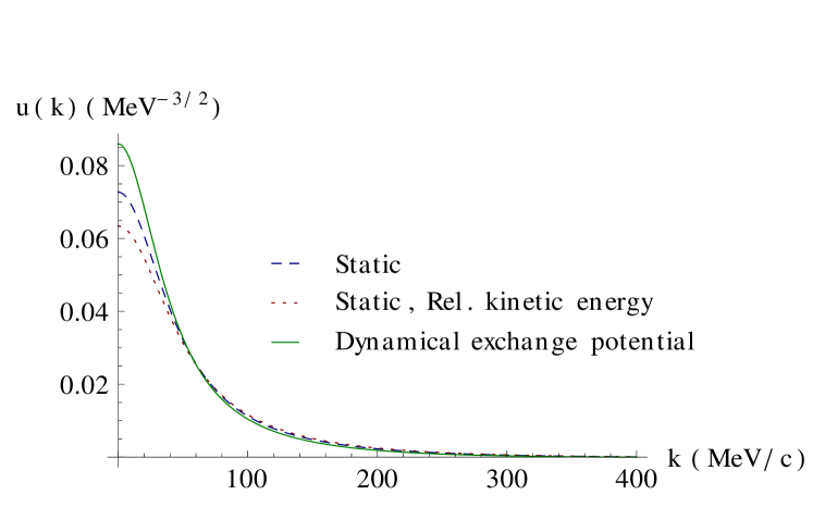
Figure 8.7: Solutions of the mass eigenvalue equation for the Walecka-type model in the non-relativistic approximation, where the kinetic energy is nonrelativistic and $\sigma$- and $\omega$-exchange are taken in the static limit [21, 64] (dashed line). It is to be compared with the same static approximation but relativistic kinetic energy [21, 64] (dotted line) and with the final result obtained within this work, were the kinetic energy is relativistic, the $\omega$-exchange is still static, but the $\sigma$-meson exchange is dynamical (solid line).

	$E_{B}$	$m_{D}$
Nonrelativistic approx. [64, 21]	-2.224575 MeV	1875.61 MeV
Relativistic kinetic energy + static potential [64, 21]	-2.73414 MeV	1875.44 MeV
Dynamical $\sigma$-exchange potential (this work)	- 1.73192 MeV	1876.1 MeV

Table 8.2: Binding energies and deuteron masses in the Walecka-type model for the static approximation of $\sigma$- and $\omega$-exchange [21] (first and second rows) with non-relativistic and relativistic kinetic energies, respectively. The third row corresponds to the dynamical treatment of the binding $\sigma$-exchange.

The first row in Table 8.2 corresponds to the nonrelativistic approximation, where the parameters of the Walecka model were calculated in such a way that the experimental values for the binding energy and the scattering length were reproduced. Replacing the kinetic energies of the nucleons by the relativistic ones, and keeping the static approximation for the interactions, one obtains the strongest binding energy, shown in the second row of Table 8.2. The calculation carried out in this work shows the relativistic effects that are due to the relativistic kinetic energies as well as the retardation of the $\sigma$-exchange (cf. Eq. (8.8)). The nucleons are less bound than in the nonrelativistic case, with the absolute value of the binding energy being approximately 22% smaller. The difference between our result and the one in the second row of Table 8.2 is the relativistic effect that is exclusively due to the retardation of the meson exchange, which reduces the binding energy by about 37%.

The $\omega$-exchange has been considered in the static approximation, as was done in previous calculations. One can guess from the previous results that the dynamical $\omega$-exchange is less repulsive than the static approximation, since in the nonrelativistic limit both, $\sigma$- and $\omega$-terms, have the same structure with opposite signs. It is therefore expectable that treating also the $\omega$-exchange dynamically leads again to a stronger binding. Nevertheless, we are not yet in the position to make a definitive conclusion since $\omega$-exchange includes also important spin effects. Regarding the wave function, as one can see, the strongest binding leads to the broadest wave function. This is reasonable, since the average constituent momentum is larger for strong binding than for weak binding.

Chapter 9 Front-form chiral multiplets

In this chapter we will present the angular-momentum decomposition of chiral multiplets in front form. This is an interesting application of the Clebsch-Gordan coefficients of the Poincaré group. We provide the unitary transformation that relates the $q\bar{q}$ chiral basis $\{R;IJ^{PC}\}$ with the nonrelativistic-inspired $\{I;^{2S+1}L_{J}\}$ classification scheme in a front-front form framework. The following discussion can also be found in Ref. [46].

In relativistic composite systems the internal degrees of freedom transform among themselves nontrivially under rotations [4]. Dirac’s forms of dynamics [2], which are defined according to the way how the interactions enter, lead to the definition of different kinds of spin bases. In relativistic quantum mechanics, any kind of spin is fully defined by a certain type of boost (cf. App. A.1.1). In this sense, one can speak about “forms” of dynamics even in the context of free systems or where the interactions can be neglected, refering to a particular basis. In particular, we refer to spin bases, on which spin states can be defined. We present an example in which the three most important kinds of spin, i.e. canonical spins, helicity spins and front-form spins, come into play in the angular momentum decomposition of chiral states. This example shows the nontriviality of the description of the angular momentum in relativistic composite systems, even in absence of interactions.

9.1 Motivation

It has been shown in Ref. [67] that there is a unitary transformation that relates the $q\bar{q}$ chiral basis, usually represented as $\{R;IJ^{PC}\}$, and the $\{I;$ ${}^{2S+1}L_{J}\}$ basis, which regards the spin-orbit angular momentum coupling used in nonrelativistic quantum mechanics. Here $R$ is the index of the chiral representation ($R=(0,0)$, $(1/2,1/2)_{a}$, $(1/2,1/2)_{b}$ or $(0,1)+(1,0)$), $I$ the quantum number of isospin, and $J^{PC}$ indicates the total angular momentum of the state with definite parity and charge. This allows one to write a particular state belonging to a chiral multiplet with quantum numbers $J^{PC}$ as a superposition of states of the nonrelativistically-inspired $\{I;^{2S+1}L_{J}\}$ classification scheme.

A chiral state with definite parity $|R;IJ^{PC}\rangle$ can be decomposed as a superposition of helicity states without definite parity $|J\lambda_{1}\lambda_{2}\rangle$ through [67, 68]

$$|R;IJ^{PC}\rangle=\sum_{\lambda_{1}\lambda_{2}}\sum_{i_{1}i_{2}}\chi^{RPI}_{\lambda_{1}\lambda_{2}}C^{Ii}_{(1/2)i_{1}(1/2)i_{2}}|i_{1}\rangle|i_{2}\rangle|J\lambda_{1}\lambda_{2}\rangle,$$ (9.1)

where $i_{1(2)}$ and $\lambda_{1(2)}$ are individual isospins and helicities respectively. The coefficients $\chi^{RPI}_{\lambda_{1}\lambda_{2}}$ relate the helicity basis to the chiral basis with definite parity in the state. They can be found in Refs. [67, 68]. $C^{JM}_{s_{1}\sigma_{1}s_{2}\sigma_{2}}$ are the usual $SU(2)$ Clebsch-Gordan coefficients.

Two-particle helicity states $|J\lambda_{1}\lambda_{2}\rangle$ can be written in terms of vectors in the $\{I;^{2S+1}L_{J}\}$ basis once one knows the expression for the matrix elements [69]

$$\langle J\lambda_{1}\lambda_{2}|^{2S+1}L_{J}\rangle=\sqrt{\frac{2L+1}{2J+1}}C^{S\Lambda}_{(1/2)\lambda_{1}(1/2)-\lambda_{2}}C^{J\Lambda}_{L0S\Lambda}.$$ (9.2)

It represents the angular momentum coupling of a two-particle state with individual helicities $\lambda_{1}$, $\lambda_{2}$ (with $\Lambda=\lambda_{1}-\lambda_{2}$; this should not be confused with the Lorentz-transformation matrix used in previous chapters) to a system of total spin $S$ and orbital angular momentum $L$.

Combining Eqs. (9.1) and (9.2) one finds

$$|R;IJ^{PC}\rangle = \sum_{LS}\sum_{\lambda_{1}\lambda_{2}}\sum_{i_{1}i_{2}}\chi^{RPI}_{\lambda_{1}\lambda_{2}}C^{Ii}_{(1/2)i_{1}(1/2)i_{2}}|i_{1}\rangle|i_{2}\rangle$$ (9.3)

$$\times\sqrt{\frac{2L+1}{2J+1}}C^{S\Lambda}_{(1/2)\lambda_{1}(1/2)-\lambda_{2}}C^{J\Lambda}_{L0S\Lambda}|^{2S+1}L_{J}\rangle.$$

As an example, the $\rho$-like state which belongs to the chiral multiplets $|(0,1)+(1,0);11^{--}\rangle$ and $|(1/2,1/2)_{b};11^{--}\rangle$ can be represented as [67]

$$|(0,1)+(1,0);11^{--}\rangle=\sqrt{\frac{2}{3}}|1;^{3}S_{1}\rangle+\sqrt{\frac{1}{3}}|1;^{3}D_{1}\rangle,$$ (9.4)

$$|(1/2,1/2)_{b};11^{--}\rangle=\sqrt{\frac{1}{3}}|1;^{3}S_{1}\rangle-\sqrt{\frac{2}{3}}|1;^{3}D_{1}\rangle.$$ (9.5)

Since both, the chiral and ${}^{2S+1}L_{J}$ representations are complete for two-particle systems with the quantum numbers $I,J^{PC}$, the angular momentum expansion is uniquely determined for each chiral state.

Chiral symmetry imposes strong restrictions on the spin and angular momentum distribution of a system. Such a decomposition has been used in Ref. [70] to test the chiral-symmetry breaking of the $\rho$ meson in the infrared, and at the same time, to reconstruct its spin and orbital angular momentum content in terms of partial waves. This was achieved by using interpolators that transform according to $|(0,1)+(1,0);11^{--}\rangle$ and $|(1/2,1/2)_{b};11^{--}\rangle$. If chiral symmetry were not broken there would be only two possible chiral states in the meson; while chiral symmetry breaking would imply a superposition of both. The obtained result in Ref. [70] indicates that the $q\bar{q}$ component of the $\rho$-meson in the infrared is indeed a superposition of the $|(0,1)+(1,0);11^{--}\rangle$ and $|(1/2,1/2)_{b};11^{--}\rangle$ chiral states, and therefore chiral symmetry turns out to be broken. By using the transformations (9.4) and (9.5) the partial wave content can be extracted, leading for the particular case of the $\rho$ meson to a nearly pure ${}^{3}S_{1}$ state [70]. This is an example for a physical application of the angular-momentum decomposition given in Eq. (9.3) (see also Refs. [67, 71]).

It is however, not the aim of this work to discuss problems in which the chiral basis or its transformation can play a role as was done in Refs. [67, 70] or [71], for instance. The problem we want to address here is more technical and related to the transformation (9.3) itself. The unitary transformation (9.3) was obtained in the instant form of relativistic quantum mechanics. In this work we investigate the corresponding expression one should use in the context of approaches that use light-front quantization [12] or front-form relativistic quantum mechanics [4]. We pose the question whether the transformation (9.3) is identical in any other form [2, 4] or if it is a special feature of those that use canonical spin, such as the instant- or the point-forms. The problem is not trivial since in relativistic composite systems the internal degrees of freedom transform among themselves nontrivially under rotations [4]. Relativity mixes spatial and temporal components and, as a consequence, one is not allowed to treat boosts and angular momentum separately in general. The election of a particular representation matters and in some cases some of the symmetry properties of the Poincaré group might not be manifest. The front form is of special interest, since rotations do not form a subgroup of the kinematical group and rotational invariance is not manifest. On the other hand, front-form boosts form a subgroup of the Poincaré group and, as a result, the front-form Wigner rotation becomes the identity [4].

In this work we will show that the unitary transformation derived in Ref. [67] in instant form is indeed identical in the front form of relativistic quantum mechanics. The argument resides in the fact that the generalized Melosh rotation that transforms front-form spins to helicity ones, becomes the identity when the mass goes to zero [72, 73, 74].

9.2 Instant-form decomposition

Due to rotational and translational invariance in nonrelativistic quantum mechanics, the angular momentum coupling of two particles with individual spin and orbital angular momentum $(\vec{s}_{1},\vec{l}_{1})$ and $(\vec{s}_{2},\vec{l}_{2})$ to a composite system of total spin and orbital angular momentum $(\vec{S},\vec{L})$ is easily realized by using the $SU(2)$ Clebsch-Gordan coefficients. Relativity involves, however, a change of representation in which the single-particle momenta and spins are replaced by an overall system momentum and internal angular momentum [4]. It is customary to use the Clebsch-Gordan coefficients of the Poincaré group [4].

The kind of spin vector can be fully determined through the choice of a certain type of boost (cf. App. A.1.1). Canonical boosts are rotationless. Spin vectors defined through canonical boosts have the advantage that in the center-of-momentum frame they transform under rotations in the same way as in nonrelativistic quantum mechanics and therefore for a composite system one can find a direct decomposition in terms of $SU(2)$ Clebsch-Gordan coefficients. The reason is that in the canonical case the Wigner rotation associated with a pure rotation turns out to be the rotation itself [4]. This does not hold in general. In the front form an angular momentum decomposition in terms of Clebsch-Gordan coefficients requires additional transformations.

Expression (9.2) can be achieved in a straightforward manner in the instant-form of dynamics, as well as in any other form that uses canonical spin. The derivation of (9.2) can be found in Ref. [69]. We will reproduce it here in a basis for the two-particle representation space of the Poincaré group in order to be able to refer the most important steps when we go to the analogous decomposition in front form in the next section. We decompose the spin part of a two-particle state with total canonical angular momentum $J$ and $\hat{z}$-component $M$, orbital angular momentum $L$ and total spin $S$, in terms of quantum numbers of the constituents in the center-of-momentum frame ($\vec{P}=\vec{0}$), where the relative momentum is expressed as $\vec{k}=\vec{k}_{1}=-\vec{k}_{2}$,

$$|[LS]|\vec{k}|J;\vec{0}\,M\rangle=\sum_{M_{L}M_{S}}\sum_{\sigma_{1}\sigma_{2}}\int d\hat{k}\,|\vec{k}\sigma_{1}-\vec{k}\sigma_{2}\rangle C^{SM_{S}}_{s_{1}\sigma_{1}s_{2}\sigma_{2}}Y_{LM_{L}}(\hat{k})\;C^{JM}_{LM_{L}SM_{S}},$$ (9.6)

where $|\vec{k}\sigma_{1}-\vec{k}\sigma_{2}\rangle:=|\vec{k}\sigma_{1}\rangle|-\vec{k}\sigma_{2}\rangle$, $s_{1(2)}$ and $\sigma_{1(2)}$ are the individual canonical spins and their $\hat{z}$-projections, respectively, and $\hat{k}=\vec{k}/|\vec{k}|$.

Given a particular direction $\hat{n}$, the tensor product state can be written as

$$\langle\hat{n}|\vec{k}\sigma_{1}-\vec{k}\sigma_{2}\rangle:=\psi_{s_{1}\sigma_{1}}(\vec{k})\psi_{s_{2}\sigma_{2}}(-\vec{k})\delta^{2}(\hat{k}-\hat{n}),$$ (9.7)

and one can introduce the wave function

$$\psi_{JLSM}(\vec{k}) := \langle\hat{n}|[LS]|\vec{k}|J;\vec{0}\,M\rangle$$

$$= \sum_{M_{L}M_{S}}\sum_{\sigma_{1}\sigma_{2}}\psi_{s_{1}\sigma_{1}}(\vec{k})\psi_{s_{2}\sigma_{2}}(-\vec{k})C^{SM_{S}}_{s_{1}\sigma_{1}s_{2}\sigma_{2}}Y_{LM_{L}}(\hat{k})\;C^{JM}_{LM_{L}SM_{S}}.$$

In order to express $\psi_{JLSM}(\vec{k})$ in terms of helicities one needs to transform states with canonical spin to a basis of states with helicity spin. The unitary transformation that provides this is a Wigner rotation whose argument corresponds to the angle between the $z$-axis and the direction of motion $\hat{k}:=\vec{k}/|\vec{k}|$

$$\psi_{s_{1}\sigma_{1}}(\vec{k})=\sum_{\lambda_{1}}D^{(s_{1})}_{\lambda_{1}\sigma_{1}}(\hat{k})\psi_{s_{1}\lambda_{1}}(\vec{k}),$$ (9.9)

$$\psi_{s_{2}\sigma_{2}}(-\vec{k})=\sum_{\lambda_{2}}D^{(s_{2})}_{-\lambda_{2}\sigma_{2}}(\hat{k})\psi_{s_{2}-\lambda_{2}}(\vec{k}).$$ (9.10)

Inserting these relations into Eq. (9.6) one gets

$$\psi_{JLSM}(\vec{k}) = \sum_{M_{S}M_{L}}\sum_{\sigma_{1}\sigma_{2}}\sum_{\lambda_{1}\lambda_{2}}D^{(s_{1})}_{\lambda_{1}\sigma_{1}}(\hat{k})\psi_{s_{1}\lambda_{1}}(\vec{k})D^{(s_{2})}_{-\lambda_{2}\sigma_{2}}(\hat{k})\psi_{s_{2}-\lambda_{2}}(\vec{k})\;$$ (9.11)

$$\times Y_{LM_{L}}(\hat{k})\;C^{SM_{S}}_{s1\sigma_{1}s2\sigma_{2}}\;C^{JM}_{LM_{L}SM_{S}}.$$

It is now convenient to write the spherical harmonics in terms of Wigner $D$-functions

$$Y_{LM_{L}}(\hat{k})=\sqrt{\frac{2L+1}{4\pi}}D^{L}_{0M_{L}}(\hat{k})$$ (9.12)

in such a way that one can make use of the relation for the product of Wigner $D$-functions with the same argument for axially symmetric systems [75],

$$D^{(j_{1})}_{\text{m}_{1}^{\prime}\text{m}_{1}}(\hat{w})D^{(j_{2})}_{\text{m}_{2}^{\prime}\text{m}_{2}}(\hat{w})=\sum_{j}C^{j\text{m}^{\prime}}_{j_{1}\text{m}_{1}^{\prime}j_{2}\text{m}_{2}^{\prime}}D^{(j)}_{\text{m}\text{m}^{\prime}}(\hat{w})C^{j\text{m}}_{j_{1}\text{m}_{1}j_{2}\text{m}_{2}},$$ (9.13)

with $\text{m}=\text{m}_{1}+\text{m}_{2}$, $\text{m}^{\prime}=\text{m}_{1}^{\prime}+\text{m}_{2}^{\prime}$, and $\hat{w}$ accounting for the Euler angles. This leads to

$$\psi_{JLSM}(\vec{k}) = \sum_{\lambda_{1}\lambda_{2}}\sqrt{\frac{2J+1}{4\pi}}D^{J}_{\Lambda M_{J}}(\hat{k})\psi_{s_{1}\lambda_{1}}(\vec{k})\psi_{s_{2}-\lambda_{2}}(\vec{k})$$ (9.14)

$$\times\sqrt{\frac{2L+1}{2J+1}}C^{S\Lambda}_{s_{1}\lambda_{1}s_{2}-\lambda_{2}}C^{J\Lambda}_{L0S\Lambda}.$$

The fact that the Wigner $D$-functions in Eq. (9.11) have the same argument is a particular feature of the instant form and it is restricted to the rest frame [4].

It is now easy to identify the needed matrix elements as

$$\psi_{JLSM}(\vec{k})=\sum_{\lambda_{1}\lambda_{2}}\psi_{JM\lambda_{1}\lambda_{2}}(\vec{k})\langle JM\lambda_{1}\lambda_{2}|^{2S+1}L_{J}M\rangle,$$ (9.15)

with

$$\psi_{JM\lambda_{1}\lambda_{2}}(\vec{k}):=\sqrt{\frac{2J+1}{4\pi}}D^{J}_{\Lambda M_{J}}(\hat{k})\psi_{s_{1}\lambda_{1}}(\vec{k})\psi_{s_{2}-\lambda_{2}}(\vec{k})$$ (9.16)

and

$$\langle JM\lambda_{1}\lambda_{2}|^{2S+1}L_{J}M\rangle=\sqrt{\frac{2L+1}{2J+1}}C^{S\Lambda}_{s_{1}\lambda_{1}s_{2}-\lambda_{2}}C^{J\Lambda}_{L0S\Lambda}.$$ (9.17)

This permits the translation from two-particle helicity states with total angular momentum $J$, to a state of overall orbital angular momentum $L$ and intrinsic spin $S$. The connection with chirality is immediately given by Eq. (9.1).

9.3 Front-form decomposition

Equation (9.6) describes the angular momentum decomposition of a representation of canonical spin into a superposition of representations with canonical spin. Because in the front form rotations do not form a subgroup of the kinematical group of the Poincaré group, the decomposition (9.6) is not feasible a priori. In order to analyze the coupling of two representations with individual spin to a superposition of representations with total spin for an arbitrary case in relativistic quantum mechanics, it is necessary to use a consistent expression of the Clebsch-Gordan coefficients of the Poincaré group [4]. Front-form angular momentum coupling is well known and it has been widely applied to hadron and nuclear problems in front-form relativistic quantum mechanics. A relation of the type (9.3), however, has not been established yet in the front form. This is the aim of the present section.

In the following we will use the normalization and notation of Ref. [4]. The light-front components of the four-momentum are defined by $\vec{\tilde{p}}:=(p^{+}=p^{0}+p^{3},\vec{p}_{\perp}=(p^{1},p^{2}))$, $p^{-}=p^{0}-p^{3}$. $|\vec{\tilde{p}}\mu\rangle_{f}$ represents a single particle state belonging to the front-form basis (labeled by $f$), with $\hat{z}$-spin projection $\mu$. The expression for the Clebsch-Gordan coefficients of the Poincaré group in the front form for an arbitrary frame is given by [4]:

$${}_{f}\langle\vec{\tilde{p}}_{1}\mu_{1}\vec{\tilde{p}}_{2}\mu_{2}|\,[LS]\,|\vec{k}|J;\vec{\tilde{P}}\,M\rangle_{f}$$

$$\quad=\delta(\vec{\tilde{P}}-\vec{\tilde{p}}_{1}-\vec{\tilde{p}}_{2})\;\frac{1}{|\vec{k}|^{2}}\delta(|\vec{k}(\vec{\tilde{p}}_{1},\vec{\tilde{p}}_{2})|-|\vec{k}|)\left|\frac{\partial(\vec{\tilde{P}},\vec{k})}{\partial(\vec{\tilde{p}}_{1},\vec{\tilde{p}}_{2})}\right|^{1/2}$$

$$\quad\times\sum_{\sigma_{1}\sigma_{2}}D^{(s_{1})}_{\mu_{1}\sigma_{1}}[\text{R}_{fc}(\vec{k},m_{1})]D^{(s_{2})}_{\mu_{2}\sigma_{2}}[\text{R}_{fc}(-\vec{k},m_{2})]$$

$$\quad\times Y^{L}_{M_{L}}(\hat{\vec{k}})C^{SM_{S}}_{s_{1}\sigma_{1}s_{2}\sigma_{2}}C^{JM}_{LM_{L}SM_{S}},$$ (9.18)

where ${}_{f}\langle\vec{\tilde{p}}_{1}\mu_{1}\vec{\tilde{p}}_{2}\mu_{2}|$ represents a tensor-product state of two particles with individual momenta $\vec{\tilde{p}}_{1}$ and $\vec{\tilde{p}}_{2}$ and spin $\hat{z}$-projections $\mu_{1}$ and $\mu_{2}$, respectively. The system of two particles moves with a total front-form momentum $\vec{\tilde{P}}$ and the individual spins couple to give a total angular momentum $J$ with orbital and spin contributions $[LS]$ in the rest frame in the canonical form, and total angular momentum projection on the $\hat{z}$-direction, $M$. Finally, $\vec{k}=\vec{k}_{1}=-\vec{k}_{2}$ is used to denote the individual momenta in the rest frame in the canonical form, and $m_{1}$ and $m_{2}$ denote the individual constituent masses (they should not be confused with the spin projections, which appear in Roman in equation (9.13)). The arguments of the Wigner $D$-functions are Melosh rotations which transform states with canonical spin to states with front-form spin and vice versa. Note that the rotation depends on the mass in general, producing a different effect on each constituent. Unless we are dealing with a system of identical constituent masses (e.g. the chiral case), we will not be able to use the properties of the $D$-function with the same argument (cf. Eq. 9.13) as was done in the instant form.

The Clebsch-Gordan coefficient (9.3) is consistent with the normalization condition for single states

$${}_{f}\langle\vec{\tilde{p}}^{\prime}\mu^{\prime}|\vec{\tilde{p}}\mu\rangle_{f}=\delta(\vec{\tilde{p}}-\vec{\tilde{p}}^{\prime})\,\delta_{\mu\mu^{\prime}}$$ (9.19)

and for state vectors of overall momentum $\vec{\tilde{P}}$

$${}_{f}\langle[L^{\prime}S^{\prime}]\,|\vec{k}^{\prime}|J^{\prime};\vec{\tilde{P}}^{\prime}\,M^{\prime}|\,[LS]\,|\vec{k}|J;\vec{\tilde{P}}\,M\rangle_{f}$$ (9.20)

$$\quad\quad=\delta_{M^{\prime}M}\delta_{J^{\prime}J}\delta_{L^{\prime}L}\delta_{S^{\prime}S}\delta(P^{\prime+}-P^{+})\delta^{2}(\vec{P}^{\prime}_{\perp}-\vec{P}_{\perp})\frac{1}{|\vec{k}|^{2}}\delta(|\vec{k}|-|\vec{k}^{\prime}|).$$

The problem now is to couple a state of total front-form angular momentum $J$ and spin projection $M$, $|[LS]|\vec{k}|,J;\vec{\tilde{P}}\,M\rangle_{f}$, to a tensor-product state of two particles with individual spins described in terms of helicities ${}_{h}\langle\vec{p}_{1}\lambda_{1}\vec{p}_{2}\lambda_{2}|$.

Irreducible representations with different types of spin are related to each other through a unitary transformation [4]. The unitary transformation that relates helicity spin to front-form spin becomes the identity for massless particles [72, 73, 74]. This means:

$$|\vec{\tilde{p}}_{1}\mu_{1}\vec{\tilde{p}}_{2}\mu_{2}\rangle_{f}\stackrel{{\scriptstyle m\to 0}}{{\longrightarrow}}\sum_{\lambda_{1}\lambda_{2}}|\vec{\tilde{p}}_{1}\lambda_{1}\vec{\tilde{p}}_{2}\lambda_{2}\rangle_{h}\delta_{\lambda_{1}\mu_{1}}\delta_{\lambda_{2}\mu_{2}},$$ (9.21)

where the subindex $h$ labels helicity states. Light-cone spins and helicity spins coincide in the chiral limit and one is allowed to make use of them without distinction. Using (9.21) in (9.3), one obtains the Clebsch-Gordan coefficient that couples two-particle helicity states to an overall state of the front-form basis,

$${}_{h}\langle\vec{\tilde{p}}_{1}\lambda_{1}\vec{\tilde{p}}_{2}\lambda_{2}|\,[LS]\,|\vec{k}|J;\vec{\tilde{P}}\,M\rangle_{f}$$

$$\quad=\delta(\vec{\tilde{P}}-\vec{\tilde{p}}_{1}-\vec{\tilde{p}}_{2})\;\frac{1}{|\vec{k}|^{2}}\;\delta(|\vec{k}(\vec{\tilde{p}}_{1},\vec{\tilde{p}}_{2})|-|\vec{k}|)\left|\frac{\partial(\vec{\tilde{P}},\vec{k})}{\partial(\vec{\tilde{p}}_{1},\vec{\tilde{p}}_{2})}\right|^{1/2}$$

$$\quad\times\sum_{\sigma_{1}\sigma_{2}}D^{(s_{1})}_{\lambda_{1}\sigma_{1}}[\text{R}_{hc}(\hat{k})]D^{(s_{2})}_{\lambda_{2}\sigma_{2}}[\text{R}_{hc}(-\hat{k})]$$

$$\quad\times Y^{L}_{M_{L}}(\hat{\vec{k}})C^{SM_{S}}_{s_{1}\sigma_{1}s_{2}\sigma_{2}}C^{JM}_{LM_{L}SM_{S}}.$$ (9.22)

Now the Melosh rotations $D^{(s_{1})}_{\lambda_{1}\sigma_{1}}[\text{R}_{hc}(\hat{k})]$ and $D^{(s_{2})}_{\lambda_{2}\sigma_{2}}[\text{R}_{hc}(-\hat{k})]$ are equivalent to the Wigner rotations and they only depend on the direction of $\vec{k}$. They have exactly the same significance as in Eq. (9.11): they transform canonical spins into helicity spins. We are now in the position to write the expression for the state in which we are interested:

$$|\,[LS]\,|\vec{k}|J;\vec{\tilde{P}}\,M\rangle_{f} = \sum_{\lambda_{1}\lambda_{2}}\int d^{3}\tilde{p}_{1}d^{3}\tilde{p}_{2}|\vec{\tilde{p}}_{1}\lambda_{1}\vec{\tilde{p}}_{2}\lambda_{2}\rangle_{h}$$ (9.23)

$$\times_{h}\langle\vec{\tilde{p}}_{1}\lambda_{1}\vec{\tilde{p}}_{2}\lambda_{2}|\,[LS]\,|\vec{k}|,J;\vec{\tilde{P}}\,M\rangle_{f},$$

where $\mathds{1}=\sum\int d^{3}\tilde{p}_{1}d^{3}\tilde{p}_{2}|\vec{\tilde{p}}_{1}\lambda_{1}\vec{\tilde{p}}_{2}\lambda_{2}\rangle_{h}\,{}_{h}\langle\vec{\tilde{p}}_{1}\lambda_{1}\vec{\tilde{p}}_{2}\lambda_{2}|$ has been introduced.

Going now to the center-of-momentum frame, $\vec{\tilde{P}}=\vec{\tilde{0}}:=(2p^{0},0,0,0)$, $\vec{\tilde{p}}_{1}=-\vec{\tilde{p}}_{2}=\vec{\tilde{k}}$, we have

$$|\,[LS]\,|\vec{k}|J;\vec{\tilde{0}}\,M\rangle_{f} = \sum_{\lambda_{1}\lambda_{2}}\sum_{\sigma_{1}\sigma_{2}}\int d\hat{\vec{k}}|\vec{k}\lambda_{1}-\vec{k}\lambda_{2}\rangle$$ (9.24)

$$\times D^{(s_{1})}_{\lambda_{1}\sigma_{1}}[\text{R}_{hc}(\hat{\vec{k}})]D^{(s_{2})}_{\lambda_{2}\sigma_{2}}[\text{R}_{hc}(-\hat{\vec{k}})]$$

$$\times Y^{L}_{M_{L}}(\hat{\vec{k}})C^{SM_{S}}_{s_{1}\sigma_{1}s_{2}\sigma_{2}}C^{JM}_{LM_{L}SM_{S}}.$$

Choosing a particular direction of relative motion $\hat{n}$, the integral over $d\hat{k}$ can be carried out by means of

$$\langle\hat{n}|\vec{k}\lambda_{1}-\vec{k}\lambda_{2}\rangle:=\psi_{s_{1}\lambda_{1}}(\vec{k})\psi_{s_{2}\lambda_{2}}(-\vec{k})\delta(\hat{k}-\hat{n})$$ (9.25)

and we define

$$\psi_{JLSM}(\vec{k}) := \langle\hat{n}|\,[LS]\,|\vec{k}|J;\vec{\tilde{0}}\,M\rangle_{f}$$ (9.26)

$$= \sum_{\lambda_{1}\lambda_{2}}\sum_{\sigma_{1}\sigma_{2}}\psi_{s_{1}\lambda_{1}}(\vec{k})\psi_{s_{2}-\lambda_{2}}(\vec{k})D^{(s_{1})}_{\lambda_{1}\sigma_{1}}[\text{R}_{hc}(\hat{k})]D^{(s_{2})}_{-\lambda_{2}\sigma_{2}}[\text{R}_{hc}(\hat{k})]$$

$$\times Y^{L}_{M_{L}}(\hat{k})C^{SM_{S}}_{s_{1}\sigma_{1}s_{2}\sigma_{2}}C^{JM}_{LM_{L}SM_{S}}.$$

Treating the spherical harmonics and the Wigner $D$-functions in the same way as in the previous section one obtains

$$\psi_{JLSM}(\vec{k})=\sum_{\lambda_{1}\lambda_{2}}\psi_{JM\lambda_{1}\lambda_{2}}(\vec{k})\langle JM\lambda_{1}\lambda_{2}|^{2S+1}L_{J}M\rangle$$ (9.27)

with

$$\psi_{JM\lambda_{1}\lambda_{2}}(\vec{k}):=\sqrt{\frac{2J+1}{4\pi}}D^{J}_{\Lambda M_{J}}(\hat{k})\psi_{s_{1}\lambda_{1}}(\vec{k})\psi_{s_{2}-\lambda_{2}}(\vec{k}),$$ (9.28)

and

$$\langle JM\lambda_{1}\lambda_{2}|^{2S+1}L_{J}M\rangle=\sqrt{\frac{2L+1}{2J+1}}C^{S\Lambda}_{s_{1}\lambda_{1}s_{2}-\lambda_{2}}C^{J\Lambda}_{L0S\Lambda}.$$ (9.29)

Having found (9.29), the validity of decomposition (9.3) is demonstrated.

Unlike in instant form, the combination of the Wigner $D$-functions would not have been possible if we had considered particles of different masses. Only in the chiral limit, or for equal masses, the eigenstates in the rest frame transform in the same way as in nonrelativistic quantum mechanics. Note that in general the coupling (9.3) involves rotations that depend on the masses, namely $D^{(s_{1})}_{\mu_{1}\sigma_{1}}[\text{R}_{fc}(\vec{k},m_{1})]$ and $D^{(s_{2})}_{\mu_{2}\sigma_{2}}[\text{R}_{fc}(-\vec{k},m_{2})]$. This would have prevented the application of Eq. (9.13), since the $D$-functions would not have the same arguments, and the dependence on the masses would have entered the decomposition, making it impossible to write Eq. (9.26) in the form of a product of (9.28) and (9.29). Moreover, a further rotation would have been necessary in order to transform front-from spins to helicity spins, which in the chiral limit turns out to be trivial by means of (9.21).

The result is that the decomposition (9.3) can also be used to expand chiral states as a superposition of vectors of the $\{I;^{2S+1}L_{J}\}$-basis within a front-form framework. They can be expressed as

$$|R;IJ^{PC}\rangle_{f} = \sum_{LS}\sum_{\lambda_{1}\lambda_{2}}\sum_{i_{1}i_{2}}\chi^{RPI}_{\lambda_{1}\lambda_{2}}C^{Ii}_{(1/2)i_{1}(1/2)i_{2}}|i_{1}\rangle|i_{2}\rangle$$ (9.30)

$$\times\sqrt{\frac{2L+1}{2J+1}}C^{S\Lambda}_{(1/2)\lambda_{1}(1/2)-\lambda_{2}}C^{J\Lambda}_{L0S\Lambda}|^{2S+1}L_{J}\rangle_{f}.$$

To summarize, we have derived the unitary transformation that relates the $q\bar{q}$ chiral basis to the $\{I;^{2S+1}L_{J}\}$-basis in a front-form framework. The result turns out to be the same as in instant form [67].

Spin vectors belonging to different representations can be related through a unitary transformation [4]. We have used the feature of the generalized Melosh rotation that relates helicity and front-form spins, which becomes the identity for massless particles. The limit $m\to 0$ eliminates the mass-dependence in the Wigner $D$-functions making it possible to express the product of $D$-functions with the same argument through a Clebsch-Gordan series for axially symmetric systems. This simplifies the the Clebsch-Gordan coefficient of the Poincaré group to an easier expression, in terms of $SU(2)$ Clebsch-Gordan coefficients.

As a last remark, let us also mention that it would have been possible to develop such a decomposition for any type of spin. The Clebsch-Gordan coefficients of the Poincaré group for an arbitrary form are given in Ref. [4]. Proceeding in an analogous way as before, it is possible to see that again the Wigner $D$-functions do not have the same argument, and it is not possible to bring them together to an overall rotation by means of $SU(2)$ Clebsch-Gordan coefficients. Only in the chiral limit the rotations are again the same. In general, a further transformation on such arbitrary spins into helicity spins is necessary to establish the relation to chirality.

Chapter 10 Summary and conclusions

Heavy-light systems with instantaneous confining forces

The first goal of this project was to extend and generalize the previous work on the electromagnetic structure of spin-0 and spin-1 two-body bound states consisting of equal-mass particles [14, 20, 21] to unequal-mass constituents and to weak decay form factors in the time-like momentum transfer region. Working within the point form of relativistic quantum mechanics and using a constituent-quark model with instantaneous confining forces we have derived electroweak current matrix elements and (transition) form factors for heavy-light mesons in the space- and time-like momentum-transfer regions. Starting point of this derivation was a multichannel formulation of the physical processes in which these form factors are measured, i.e electron-meson scattering and semileptonic weak decays. This formulation accounts fully for the dynamics of the exchanged gauge boson ($\gamma$ or $W$). Poincaré invariance is guaranteed by adopting the Bakamjian-Thomas construction with gauge-boson-fermion vertices taken from quantum field theory. Vector and axial-vector currents of the mesons can then be uniquely identified from the one-boson-exchange ($\gamma$ or $W$) amplitudes. These currents have already the right Lorentz-covariance properties and the electromagnetic current of any pseudoscalar meson is conserved. But wrong cluster properties, inherent in the Bakamjian-Thomas construction [4], give rise to spurious dependencies of the electromagnetic current on the electron momenta. For pseudoscalar mesons these unwanted dependencies are eliminated by taking the invariant mass of the electron-meson system large enough [14, 20, 21]. The resulting electromagnetic form factor of a pseudoscalar meson is then equivalent to the one obtained in front form from the $+$-component of a one-body current in a $q^{+}=0$ frame. The weak pseudoscalar-to-pseudoscalar and pseudoscalar-to-vector transition currents are not plagued by such spurious contributions. They can be expressed in terms of physical covariants and form factors with the form factors depending on the (time-like) momentum transfer squared, as it should be. In front form one observes some frame dependence of the $B\rightarrow D^{\ast}$ decay form factors if they are extracted from the $+$-component of a simple one-body current [34]. This is attributed to a missing non-valence ($Z$-graph) contribution, which makes the triangle diagram, from which the form factors are calculated, covariant [34, 37]. In the case of the point form it is, of course, also not excluded that $Z$-graphs may play a role, but they are not necessary to ensure covariance of the current, since Lorentz boosts are purely kinematical and thus do not mix in higher Fock states.

Having derived comparably simple analytical expressions for the electromagnetic form factor of a pseudoscalar heavy-light meson and the $B\rightarrow D^{(\ast)}$ decay form factors we discussed the heavy-quark limit. We found that the decay form factors (multiplied with appropriate kinematical factors) go over into one universal function, the Isgur-Wise function, as demanded by heavy-quark symmetry. For the electromagnetic form factors we observed that the heavy-quark limit does not completely remove the spurious dependence on the electron momentum. One still has a spurious covariant and the $s$-dependence of the form factors goes over into a dependence on the (common) modulus of the incoming and outgoing 3-velocities of the heavy meson. This dependence on the modulus of the meson velocities vanishes by taking it large enough. In the limit of infinitely large meson velocities we found a rather simple analytical expression for the Isgur-Wise function which turned out to be (apart from a change of integration variables) the same as the expression which we got from the decay form factors. Interestingly, we have also got the same result for the Isgur-Wise function for the minimum value of the meson velocities that is necessary to reach a particular value of $v\cdot v^{\prime}$ (the argument of the Isgur-Wise function). For minimum velocities it is not possible to separate physical and spurious contributions since the respective covariants become proportional. The dependence of the electromagnetic pseudoscalar meson form factor on Mandelstam-$s$ and the dependence of the resulting Isgur-Wise function on the modulus of the meson velocities may be interpreted as a frame dependence of the $\gamma^{\ast}M\rightarrow M$ subprocess. The $s\rightarrow\infty$ (velocities $\rightarrow\infty$) limit corresponds to the infinite-momentum frame, whereas minimum $s$ (minimum velocities) corresponds to the Breit frame. Our finding thus means that it does not matter whether we calculate the Isgur-Wise function in the infinite-momentum frame or the Breit frame. In the heavy-quark limit the results are the same and agree with the heavy-quark limit of the decay form factors. Numerical agreement was also found with the front-form calculation of Ref. [34].

As a first application and numerical check of our approach we have calculated electromagnetic $D^{+}$- and $B^{-}$ form factors, the $B\rightarrow D^{(\ast)}$ decay form factors and the Isgur-Wise function with a simple (flavor independent) Gaussian wave function. For the electromagnetic $B^{-}$ form factor and for the $B\rightarrow D^{(\ast)}$ decay form factors the effect of heavy-quark symmetry breaking due to finite physical masses of the heavy quarks turned out be $15-20\%$. For the electromagnetic $D^{+}$ form factor it rather amounted to about $60\%$.

Discrepancies between the point and front-form approach show up as soon as the decay form factors are calculated for finite, physical masses of the heavy-quarks. We have also applied our formalism to several heavy-to-heavy and heavy-to-light transition form factors using a flavor-dependent Gaussian wave function and compared our results with the front-form calculation of Ref. [34], with identical parameters. For finite quark masses differences between the front-form and the point-form approach are observed. These differences increase with decreasing quark masses. Most likely, they can be attributed to the different roles played by $Z$-graphs, i.e. non-valence contributions, in either approach. In the heavy-quark limit $Z$-graphs do not contribute to the current, neither in the front form nor in the point form, which explains why the results agree for the Isgur-Wise function. For finite quark masses, however, the inclusion of $Z$-graphs seems to be crucial for the frame independence of the decay form factors in front form, whereas it is not the case in the point form (as discussed above).

Our approach is general enough to deal with additional dynamical degrees of freedom, such that it is possible to consider non-valence Fock-state contributions in the meson [42]. It will be the topic of future work to investigate the role of $Z$-graph contributions, which indeed can be easily accommodated within our multichannel approach. It could help to reduce the spurious dependencies of the electromagnetic current on the electron momenta. It might explain, e.g., the discrepancy between the electromagnetic form factors calculated in the infinite-momentum frame and in the Breit frame for the $B^{-}$ and $D^{+}$ mesons (see Fig. 6.5).

To conclude this part, we have presented a relativistic point-form formalism for the calculation of the electroweak structure of heavy-light mesons within constituent quark models with instantaneous confining forces. This formalism provides the electromagnetic form factor of pseudoscalar heavy-light systems for space-like momentum transfers and weak pseudoscalar-to-pseudoscalar as well as pseudoscalar-to-vector decay form factors for time-like momentum transfers. It exhibits the correct heavy-quark-symmetry properties in the heavy-quark limit.

Dynamical binding forces

Another goal of this thesis was to generalize the point-form approach to systems that are bound by dynamical particle-exchange. We have considered relativistic effects coming from the retardation of a dynamical particle-exchange interaction. We have investigated such retardation effects for electron-deuteron scattering taking a Walecka-type model for the deuteron, where the binding is caused by $\sigma$- and $\omega$-exchanges. With the approximation that only the $\sigma$-exchange is considered dynamically, whereas the $\omega$-exchange is still taken in the static limit, we have obtained the relativistic wave function for the deuteron and we have studied the relativistic effects that modify the binding energy as compared with the static approximation of the $\sigma$-exchange  [21, 64]. The retardation of the $\sigma$ reduces the binding energy and enhances the small-$k$ part of the wave function. The next goal would be to examine how large the effects of exchange currents to the form factors are and whether they restore (partly) the cluster properties and reduce the spurious form factors as sometimes suspected.

Chiral multiplets in relativistic quantum mechanics

Because in relativistic composite systems the internal degrees of freedom transform among themselves nontrivially under rotations, we have emphasized the importance of considering the Clebsch-Gordan coefficients of the Poincaré group in the spin coupling of relativistic composite systems [4]. The Clebsch-Gordan coefficients of the Poincaré group convert, through an intermediate step, any kind of spin to canonical spin in the rest frame, in such a way that they can be added using $SU(2)$ Clebsch-Gordan coefficients.

Considering the Clebsch-Gordan coefficients of the Poincaré group and making use of the known property of the front-form spin, that becomes equivalent to helicity in the chiral limit, we have presented the angular momentum decomposition of chiral multiplets in an instant-form and in a front-form basis. We have shown that such decompositions are identical for massless particles. With such a unitary transformation it is possible to relate the $q\bar{q}$ chiral basis $\{R;IJ^{PC}\}$ with the nonrelativistically-inspired $\{I;^{2S+1}L_{J}\}$ classification scheme as it was done in Ref. [70] for the purpose of studying the angular momentum content of the rho-meson in lattice QCD. Although such decompositions are possible in any other spin basis, they are not identical to the both presented here in general, since an additional rotation is necessary to establish the connection with chirality.

Appendix A Notation and conventions

We present here some more details about the conventions and notations used in this work. Some basic facts about the Poincaré group and the covering group of the Poincaré group which we need repeatedly are summarized. The appendix is not intended as detailed explanation on how to construct operators, etc., within relativistic quantum mechanics. For a more comprehensive presentation we refer to Ref. [4], which we are following.

A.1 Notation

We use the Einstein convention on summation. Thereby repeated indices are implicitly summed over ($a^{i}b^{i}:=\sum_{i}a^{i}b^{i}$ ). Repeated Lorentz (Greek) indices are used to express the scalar product in Minkowski space:

$$a\cdot b:=a^{\mu}b_{\mu}=g^{\mu\nu}a_{\mu}b_{\nu}=a^{0}b^{0}-a^{i}b^{i},$$ (A.1)

with $\mu,\nu=0,1,2,3$. Latin indices are reserved for the spatial vector components. The metric tensor $g^{\mu\nu}$ of the Minkowski space is:

$$g^{00}=-g^{11}=-g^{22}=-g^{33}=1.$$ (A.2)

In general, the kinetic energy of a particle with mass $m$ and 3-momentum $\vec{k}$ is represented as:

$$\omega_{k}:=\sqrt{m^{2}+\vec{k}^{2}}.$$ (A.3)

The units we use are such that $\hbar=c=1$.

A.1.1 The Poincaré group

A Poincaré transformation on a 4-vector $x^{\mu}$ belonging to the Minkowski space is represented by

$$x^{\mu}\to x^{\prime\mu}=\Lambda^{\mu}_{\phantom{\nu}\nu}x^{\nu}+a^{\mu},$$ (A.4)

where $a^{\mu}$ is a constant 4-vector that represents a space-time translation and $\Lambda^{\mu}_{\phantom{\nu}\nu}$ is a constant $(4\times 4)$-matrix that represents a Lorentz transformation. $\Lambda^{\mu}_{\phantom{\nu}\nu}$ leaves the metric invariant:

$$g^{\mu\nu}=\Lambda^{\mu}_{\phantom{\nu}\rho}\Lambda^{\nu}_{\phantom{\nu}\sigma}g^{\rho\sigma}.$$ (A.5)

The composition of two Poincaré transformations is given by

$$(\Lambda_{2},a_{2})\circ(\Lambda_{1},a_{1})=(\Lambda_{2}\Lambda_{1},\Lambda a_{1}+a_{2}).$$ (A.6)

and the inverse and identity are

$$(\Lambda,a)^{-1}=(\Lambda^{-1},-\Lambda^{-1}a),\qquad I=(\mathds{1},0).$$ (A.7)

Commuting self-adjoint operators

The only two commuting self-adjoint operators that can be constructed as independent polynomial functions of the generators of the Poincaré group, and then be used to label irreducible representations of the Poincaré group are the square of the mass operator $\hat{M}^{2}$ and the square of the Pauli-Lubansky operator $\hat{W}^{2}:=-\hat{M}^{2}\hat{j}^{2}$, with $\hat{j}^{2}$ being the total spin operator of the system. They are the Casimir operators of the Poincaré group and are defined as follows:

$$\hat{M}:=\sqrt{\hat{P}^{\mu}\hat{P}_{\mu}},\qquad\hat{W}^{\mu}:=-\frac{1}{2}\varepsilon^{\mu\alpha\beta\gamma}\hat{P}_{\alpha}\hat{J}_{\beta\gamma},$$ (A.8)

with $\hat{P}^{\mu}$ being the generators of space-time translations and $\hat{J}^{\mu\nu}$ the antisymmetric tensor operator that contains the rotations and boost generators, $\hat{J}^{i}$ ($=\frac{1}{2}\epsilon^{ijk}\hat{J}^{jk}$) and $\hat{K}^{i}$ ($=\hat{J}^{0i}$), respectively.

Boosts

There is an infinite number of vector valued functions of the generators that satisfy the angular-momentum algebra and thus could serve as spin vectors. It is thus necessary to specify the type of spin one refers to. The type of spin can be distinguished by how they transform under Lorentz boosts. Any kind of spin can be defined by a certain type of boost.

The boost operators $B_{g}^{-1}(\hat{V})^{\nu}_{\phantom{\nu}\mu}$ (where $\hat{V}:=\hat{P}/\hat{M}$ is the four-velocity operator) represent Lorentz transformations that map $\hat{P}^{\mu}$ to $(\hat{M},0,0,0)$ and have the properties [4]:

$$B_{g}(\hat{V})^{\mu}_{\phantom{\nu}\nu}(1,0,0,0)^{\nu}=\hat{M}^{-1}\hat{P}^{\mu}$$ (A.9)

$$\hat{B}_{g}(\hat{1},0,0,0)^{\nu}_{\phantom{\nu}\mu}=g^{\nu}_{\phantom{\nu}\mu}$$ (A.10)

These relations have to be understood as operator relations. The subscript $g$ denotes the type of boost used to define the spin. The most relevant types of boost are canonical boosts, $B_{c}$, helicity boosts, $B_{h}$, and front-form boosts, $B_{f}$.

Canonical boosts are rotationless and are used in the instant form and in the point form. The action of a canonical boost with 4-velocity $v^{\mu}$ (rapidity $\omega=\text{arcsinh}|\vec{v}|$, $v_{\mu}v^{\mu}$=1) on 4-vectors in Minkowski space is described by the matrix:

$$B_{c}(v):=\left(\begin{array}[]{cc}v^{0}&\vec{v}^{T}\\ \vec{v}&\mathds{1}+\frac{v^{0}-1}{\vec{v}^{2}}\vec{v}\vec{v}^{T}\end{array}\right)$$ (A.11)

Helicity boosts are defined as a canonical boost in the $\hat{z}$-direction to the velocity of desired magnitude $|\vec{v}|$, followed by a rotation to the axis that defines the direction of the velocity ($\hat{\vec{v}}=\vec{v}/|\vec{v}|$):

$$B_{h}(v)=R(\hat{z}\to\hat{v})B_{c}(|\vec{v}|\hat{z}).$$ (A.12)

(the hat here denotes unitary vectors). Finally, front-form boosts are Lorentz transformations that leave the light-front $x^{+}=0$ invariant. They form a subgroup of the Poincaré group. Introducing light-cone coordinates $a^{\pm}=(a^{+}\pm a^{-})$ and $a_{\perp}=(a^{1},a^{2})$, the action of a front-form boost on a 4-vector $\tilde{a}=(a^{+},a_{\perp},a^{-})$, represented in these coordinates, is given by:

$$B_{f}(v)=\frac{1}{\sqrt{v^{+}}}\left(\begin{array}[]{ccc}v^{+}&v_{\perp}^{T}&0\\ v_{\perp}&\mathds{1}&0\\ v_{\perp}^{2}/v^{+}&2v_{\perp}^{T}/v^{+}&1/v^{+}\end{array}\right)$$ (A.13)

Spin vectors

A spin vector of the type $g$ is fully determined by the corresponding kind of boost $g$, i.e.

$$(0,\hat{\vec{j}}_{g}):=\frac{1}{\hat{M}}B_{g}^{-1}(\hat{V})^{\mu}_{\phantom{\nu}\nu}\hat{W}^{\nu}.$$ (A.14)

Using the inverse of the boost operator it is possible to express $\hat{\vec{j}}_{g}$ in terms of $\hat{W}^{\nu}$. Applying thus another type of boost that maps $\hat{P}^{\mu}$ to the rest frame (cf. Eq. A.9) one ends up with another type of spin. In this way one finds a relation between two kinds of spin, which turns out to be:

$$\hat{j}^{j}_{a}=B^{-1}_{a}(\hat{V})^{j}_{\phantom{j}\nu}B_{b}(\hat{V})^{\nu}_{\phantom{j}k}\hat{j}^{k}_{b}=R_{ab}(\hat{V})^{j}_{\phantom{j}k}\hat{j}^{k}_{b}.$$ (A.15)

The rotation $R_{cf}$ that transforms canonical spins $c$ into front-form spins $f$, or vice versa, is called Melosh rotation [76]. The general transformation is customary called generalized Melosh rotation.

In summary, the notation and properties of the different types of boost and their associated spins are given by

Type of boost	Subscript	Properties
canonical	$c$	rotationless
front form	$f$	they form a subgroup
helicity	$h$	$B_{h}(v)=R(\hat{z}\to\hat{v})B_{c}(|\vec{v}|\hat{z})$
any other	$g$	-

A.1.2 The covering group of the Poincaré group

Elements of the covering group of the Poincaré group $ISL(2,\mathds{C})$ (or inhomogeneous $SL(2,\mathds{C})$) are $2\times 2$ matrices ($\underline{\Lambda},\underline{a}$) with $\det{(\underline{\Lambda})}=1$ and $\underline{a}$ Hermitian [48]. Whereas the Poincaré group acts on 4-vectors belonging to the Minkowski space, the covering group of the Poincaré group acts on spin vectors belonging to the spin space. The relation between both groups can be understood through the relation between the space-time coordinate $x^{\mu}$ and the corresponding $2\times 2$ Hermitian matrix [4]:

$$\underline{X}:=x^{\mu}\sigma_{\mu}=\left(\begin{array}[]{cc}x^{0}+x^{3}&x^{1}-ix^{2}\\ x^{1}+ix^{2}&x^{0}-x^{3}\end{array}\right),\qquad x^{\mu}=\frac{1}{2}\text{Tr}(\sigma_{\mu}\underline{X}),$$ (A.16)

where $\sigma_{\mu}$ are the Pauli matrices (including $\sigma_{0}=\mathds{1}_{2\times 2}$). A Poincaré transformation is given by

$$\underline{X}\to\underline{X}^{\prime}=\underline{\Lambda}\,\underline{X}\,\underline{\Lambda}^{\dagger}+\underline{a}.$$ (A.17)

A composition of two $(\underline{\Lambda},\underline{a})$ transformations is then:

$$(\underline{\Lambda}_{2},\underline{a}_{2})\circ(\underline{\Lambda}_{1},\underline{a}_{1})=(\underline{\Lambda}_{2}\underline{\Lambda}_{1},\underline{\Lambda}_{2}\underline{a}_{1}\underline{\Lambda}_{2}^{\dagger}+\underline{a}_{2}),$$ (A.18)

and the inverse:

$$(\underline{\Lambda},\underline{a})^{-1}=(\underline{\Lambda}^{-1},-\underline{\Lambda}^{-1}\underline{a}(\underline{\Lambda}^{\dagger})^{-1}).$$ (A.19)

The relation between $(\Lambda^{\mu}_{\phantom{\mu}\nu},a)$ and $(\underline{\Lambda},\underline{a})$ is given by:

$$\Lambda^{\mu}_{\phantom{\mu}\nu}:=\frac{1}{2}\text{Tr}(\sigma_{\mu}\underline{\Lambda}\sigma_{\nu}\underline{\Lambda}^{\dagger}),\quad\text{and}\quad a^{\mu}=\frac{1}{2}\text{Tr}(\sigma_{\mu}\underline{a}).$$ (A.20)

Hence, the canonical boost matrix belonging to the covering group of the Poincaré group is given by:

$$\underline{B}_{c}(v):=\sqrt{\frac{v^{0}+1}{2}}\sigma^{0}+\frac{\vec{\sigma}\cdot\vec{v}}{\sqrt{2(v^{0}+1)}}.$$ (A.21)

The Wigner rotation defined by means of canonical boosts is in this case

$$\underline{R}_{W}(v,\underline{\Lambda})=\underline{B}_{c}^{-1}(\Lambda v)\,\underline{\Lambda}\,\underline{B}_{c}(v).$$ (A.22)

In order to simplify the notation, since elements of the $ISL(2,\mathds{C})$ can be expressed as a function of elements of the Poincaré group, we have avoided the underline in all the expressions.

Polarization vectors

The polarization vectors $\epsilon^{\mu}(\vec{0},\sigma)$ of a spin-1 particle with spin projection $\sigma$ are defined at rest by

$$\epsilon(\vec{0},0) := (0,0,0,1);$$ (A.23)

$$\epsilon(\vec{0},\pm 1) := \mp\frac{1}{\sqrt{2}}(0,1,\pm i,0).$$ (A.24)

Considering polarization vectors in an arbitrary frame requires to perform a boost, that in our case is canonical (cf. Eq. A.11):

$$\epsilon^{\mu}(\vec{k},\sigma)=B_{c}(v)^{\mu}_{\phantom{\nu}\nu}\epsilon^{\nu}(\vec{0},\sigma).$$ (A.25)

A.1.3 Field operators

For the calculation of the vertex matrix elements, e.g. Eq. (B.3), from the corresponding interaction Lagrangian densities we need the plane-wave expansions of spin-$\frac{1}{2}$ and spin-1 field operators.

Dirac field

$$\hat{\psi}(x)=\sum_{\sigma=\pm\frac{1}{2}}\int\frac{d^{3}p}{(2\pi)^{3}2\omega_{p}}\left(e^{ip\cdot x}\;v_{\sigma}(\vec{p})\;\hat{d}^{\dagger}_{\sigma}(\vec{p})+e^{-ip\cdot x}\;u_{\sigma}(\vec{p})\;\hat{c}_{\sigma}(\vec{p})\right),$$ (A.26)

$$\hat{\bar{\psi}}(x)=\sum_{\sigma=\pm\frac{1}{2}}\int\frac{d^{3}p}{(2\pi)^{3}2\omega_{p}}\left(e^{-ip\cdot x}\;\bar{v}_{\sigma}(\vec{p})\;\hat{d}_{\sigma}(\vec{p})+e^{ip\cdot x}\;\bar{u}_{\sigma}(\vec{p})\;\hat{c}_{\sigma}^{\dagger}(\vec{p})\right).$$ (A.27)

Maxwell field

$$\hat{A}^{\mu}(x)=\sum_{\sigma=0}^{3}\int\frac{d^{3}p}{(2\pi)^{3}2\omega_{p}}(-g^{\sigma\sigma})\left(e^{ip\cdot x}\;\epsilon^{\mu}(\vec{p},\sigma)\hat{a}^{\dagger}_{\sigma}(\vec{p})+e^{-ip\cdot x}\;\epsilon^{*\mu}(\vec{p},\sigma)\;\hat{a}_{\sigma}(\vec{p})\right).$$ (A.28)

Dirac spinors

Spinors and the Dirac matrices are taken in the Dirac representation:

$$u_{\rho}(\vec{k})=\sqrt{\omega_{k}+m}\left(\begin{array}[]{c}\varsigma_{\rho}\\ \frac{\vec{\sigma}\cdot¸\vec{k}}{\omega_{k}+m}\varsigma_{\rho}\end{array}\right),\;v_{\rho}=\-\sqrt{\omega_{k}+m}\left(\begin{array}[]{c}\frac{\vec{\sigma}\cdot\vec{p}}{\omega_{k}+m}\varepsilon\varsigma_{\rho}\\ \varepsilon\varsigma_{\rho}\end{array}\right),$$ (A.29)

$$\varepsilon=i\sigma_{2},\quad\varsigma_{\rho}=\left(\begin{array}[]{c}\frac{1}{2}+\rho\\ \frac{1}{2}-\rho\end{array}\right).$$ (A.30)

Dirac matrices

$$\gamma^{0}=\left(\begin{array}[]{cc}\mathds{1}&0\\ 0&-\mathds{1}\end{array}\right),\quad\vec{\gamma}=\gamma^{0}\vec{\alpha}=\left(\begin{array}[]{cc}0&\vec{\sigma}\\ -\vec{\sigma}&0\end{array}\right),\quad$$ (A.31)

$$\gamma^{5}=\left(\begin{array}[]{cc}0&\mathds{1}\\ \mathds{1}&0\end{array}\right),\quad\vec{\alpha}=\left(\begin{array}[]{cc}0&\vec{\sigma}\\ \vec{\sigma}&0\end{array}\right).$$ (A.32)

Appendix B Matrix elements

The following matrix elements are needed for the computation of matrix elements of the optical potential that describes the one-photon-exchange scattering process given in Eq. (3.1). They are inner products of free and cluster velocity states, consistent with the normalization given by Eq. (2.3.2). $\alpha$ represents the discrete quantum numbers of the $q\bar{q}$ cluster, i.e. $(n,j,\tilde{m}_{j},[\tilde{l},\tilde{s}])$, see also Refs. [18, 21]. For example, for a pseudoscalar meson we consider $(n,0,0,[0,0])$, and for a vector meson we will have $(n,1,\tilde{m}_{j},[0,1])$. This affects the Clebsch-Gordan coefficients, and the subindices in the Wigner $D$-functions. For weak decays we will write these quantum numbers explicitly, to distinguish pseudoscalar-to-pseudoscalar from pseudoscalar-to-vector transitions.

B.1 Electromagnetic scattering

For electron scattering off a meson with spin $j$ we have used for the computations of Sec. 3.1:

$$\langle v;\vec{k}_{e},\mu_{e};\vec{k}_{q},\mu_{q};\vec{k}_{\bar{q}},\mu_{\bar{q}}|\,\underline{v};\vec{\underline{k}}_{e},\underline{\mu}_{e};\vec{\underline{k}}_{\alpha},\underline{\mu}_{\alpha},\alpha\rangle$$

$$\quad=(2\pi)^{15/2}\underline{v}_{0}\delta^{3}(\vec{v}-\underline{\vec{v}})\delta^{3}(\vec{k}_{e}-\underline{\vec{k}}_{e})\delta_{\mu_{e}\underline{\mu}_{e}}$$

$$\qquad\times\sqrt{\frac{2\omega_{\underline{k}_{e}}2\omega_{\underline{k}_{\alpha}}}{(\omega_{\underline{k}_{e}}+\omega_{\underline{k}_{\alpha}})^{3}}}\sqrt{\frac{2\omega_{k_{e}}2\omega_{\underline{k}_{q\bar{q}}}}{(\omega_{k_{e}}+\omega_{\underline{k}_{q\bar{q}}})^{3}}}\sqrt{\frac{2\omega_{\tilde{k}_{q}}2\omega_{\tilde{k}_{\bar{q}}}}{(\omega_{\tilde{k}_{q}}+\omega_{\tilde{k}_{\bar{q}}})}}$$

$$\qquad\times\sum_{\tilde{m}_{l}=-\tilde{l}}^{\tilde{l}}\sum_{\tilde{m}_{s}=-\tilde{s}}^{\tilde{s}}\sum_{\tilde{\mu}_{q}\tilde{\mu}_{\bar{q}}=\pm 1/2}C^{j\tilde{m}_{j}}_{\tilde{l}\tilde{m}_{l}\tilde{s}\tilde{m}_{s}}C^{\tilde{s}\tilde{m}_{s}}_{\frac{1}{2}\tilde{\mu}_{q}\frac{1}{2}\tilde{\mu}_{\bar{q}}}\;u_{n\tilde{l}}(|\vec{\tilde{k}}_{q}|)Y_{\tilde{l}\tilde{m}_{l}}(\hat{\tilde{k}}_{q})$$

$$\qquad\times D^{1/2}_{\mu_{q}\tilde{\mu}_{q}}\left[R_{W}\left(\frac{\tilde{k}_{q}}{m_{q}},B_{c}(v_{q\bar{q}})\right)\right]D^{1/2}_{\mu_{\bar{q}}\tilde{\mu}_{\bar{q}}}\left[R_{W}\left(\frac{\tilde{k}_{\bar{q}}}{m_{\bar{q}}},B_{c}(v_{q\bar{q}})\right)\right],$$

$$\langle v;\vec{k}_{e},\mu_{e};\vec{k}_{q},\mu_{q};\vec{k}_{\bar{q}},\mu_{\bar{q}};\vec{k}_{\gamma},\mu_{\gamma}|\,\underline{v};\vec{\underline{k}}_{e},\underline{\mu}_{e};\vec{\underline{k}}_{\alpha},\underline{\mu}_{\alpha};\vec{\underline{k}}_{\gamma},\underline{\mu}_{\gamma};\alpha\rangle$$

$$\quad=(2\pi)^{21/2}\underline{v}_{0}\delta^{3}(\vec{v}-\underline{\vec{v}})\delta^{3}(\vec{k}_{e}-\underline{\vec{k}}_{e})\delta_{\mu_{e}\underline{\mu}_{e}}\delta^{3}(\vec{k}_{\gamma}-\underline{\vec{k}}_{\gamma})(-g_{\mu_{\gamma}\underline{\mu}_{\gamma}})$$

$$\qquad\times\sqrt{\frac{2\omega_{\underline{k}_{e}}2\omega_{\underline{k}_{\alpha}}2\omega_{\underline{k}_{\gamma}}}{(\omega_{\underline{k}_{e}}+\omega_{\underline{k}_{\alpha}}+\omega_{\underline{k}_{\gamma}})^{3}}}\sqrt{\frac{2\omega_{k_{e}}2\omega_{\underline{k}_{q\bar{q}}}2\omega_{\underline{k}_{\gamma}}}{(\omega_{k_{e}}+\omega_{\underline{k}_{q\bar{q}}}+\omega_{\underline{k}_{\gamma}})^{3}}}\sqrt{\frac{2\omega_{\tilde{k}_{q}}2\omega_{\tilde{k}_{\bar{q}}}}{(\omega_{\tilde{k}_{q}}+\omega_{\tilde{k}_{\bar{q}}})}}$$

$$\qquad\times\sum_{\tilde{m}_{l}=-\tilde{l}}^{\tilde{l}}\sum_{\tilde{m}_{s}=-\tilde{s}}^{\tilde{s}}\sum_{\tilde{\mu}_{q}\tilde{\mu}_{\bar{q}}=\pm 1/2}C^{j\tilde{m}_{j}}_{\tilde{l}\tilde{m}_{l}\tilde{s}\tilde{m}_{s}}C^{\tilde{s}\tilde{m}_{s}}_{\frac{1}{2}\tilde{\mu}_{q}\frac{1}{2}\tilde{\mu}_{\bar{q}}}\;u_{n\tilde{l}}(|\vec{\tilde{k}}_{q}|)Y_{\tilde{l}\tilde{m}_{l}}(\hat{\tilde{k}}_{q})$$

$$\qquad\times D^{1/2}_{\mu_{q}\tilde{\mu}_{q}}\left[R_{W}\left(\frac{\tilde{k}_{q}}{m_{q}},B_{c}(v_{q\bar{q}})\right)\right]D^{1/2}_{\mu_{\bar{q}}\tilde{\mu}_{\bar{q}}}\left[R_{W}\left(\frac{\tilde{k}_{\bar{q}}}{m_{\bar{q}}},B_{c}(v_{q\bar{q}})\right)\right],$$

$$\langle v^{\prime};\vec{k}_{e}^{\prime},\mu_{e}^{\prime};\vec{k}_{q}^{\prime},\mu_{q}^{\prime};\vec{k}_{\bar{q}}^{\prime},\mu_{\bar{q}}^{\prime};\vec{k}_{\gamma}^{\prime},\mu_{\gamma}^{\prime}|\,\hat{K}_{\gamma}^{\dagger}\,|v;\vec{k}_{e},\mu_{e};\vec{k}_{q},\mu_{q};\vec{k}_{\bar{q}},\mu_{\bar{q}}\rangle$$ (B.3)

$$= \langle v;\vec{k}_{e},\mu_{e};\vec{k}_{q},\mu_{q};\vec{k}_{\bar{q}},\mu_{\bar{q}}|\,\hat{K}_{\gamma}\,|v^{\prime};\vec{k}_{e}^{\prime},\mu_{e}^{\prime};\vec{k}_{q}^{\prime},\mu_{q}^{\prime};\vec{k}_{\bar{q}}^{\prime},\mu_{\bar{q}}^{\prime};\vec{k}_{\gamma}^{\prime},\mu_{\gamma}^{\prime}\rangle^{*}$$

$$= v_{0}\,\delta^{3}(\vec{v}^{\prime}-\vec{v})\,\frac{(2\pi)^{3}}{\sqrt{(\omega_{k_{e}^{\prime}}+\omega_{k_{q}^{\prime}}+\omega_{k_{\bar{q}}^{\prime}}+\omega_{k_{\gamma}^{\prime}})^{3}}\sqrt{(\omega_{k_{e}}+\omega_{k_{q}^{\phantom{\prime}}}+\omega_{k_{\bar{q}}})^{3}}}$$

$$\times\langle\vec{k}_{e}^{\prime},\mu_{e}^{\prime};\vec{k}_{q}^{\prime},\mu_{q}^{\prime};\vec{k}_{\bar{q}}^{\prime},\mu_{\bar{q}}^{\prime};\vec{k}_{\gamma}^{\prime},\mu_{\gamma}^{\prime}|\,\left(\hat{\mathcal{L}}_{\mathrm{int}}^{e\gamma}(0)+\hat{\mathcal{L}}_{\mathrm{int}}^{q\gamma}(0)\right)|\vec{k}_{e},\mu_{e};\vec{k}_{q},\mu_{q};\vec{k}_{\bar{q}},\mu_{\bar{q}}\rangle$$

$$= v_{0}\,\delta^{3}(\vec{v}^{\prime}-\vec{v})\,\frac{(2\pi)^{3}}{\sqrt{(\omega_{k_{e}^{\prime}}+\omega_{k_{M}^{\prime}}+\omega_{k_{\gamma}^{\prime}})^{3}}\sqrt{(\omega_{k_{e}}+\omega_{k_{M}^{\phantom{\prime}}})^{3}}}(-1)$$

$$\times\left[\,Q_{e}\,\bar{u}_{\mu_{e}^{\prime}}(\vec{k}_{e}^{\prime})\gamma_{\nu}u_{\mu_{e}}(\vec{k}_{e})\,\epsilon^{\nu}(\vec{k}_{\gamma}^{\prime},\mu_{\gamma}^{\prime})\,(2\pi)^{3}2\omega_{k_{q}}\delta^{3}(\vec{k}_{q}^{\prime}-\vec{k}_{q})\delta_{\mu_{q}\mu^{\prime}_{q}}\,\right.$$

$$\left.\;\;\qquad\times(2\pi)^{3}2\omega_{k_{\bar{q}}}\delta^{3}(\vec{k}_{\bar{q}}^{\prime}-\vec{k}_{\bar{q}})\delta_{\mu_{\bar{q}}\mu^{\prime}_{\bar{q}}}\right.$$

$$\left.\;\;+\,Q_{q}\,\bar{u}_{\mu_{q}^{\prime}}(\vec{k}_{q}^{\prime})\gamma_{\nu}u_{\mu_{q}}(\vec{k}_{q})\,\epsilon^{\nu}(\vec{k}_{\gamma}^{\prime},\mu_{\gamma}^{\prime})\,(2\pi)^{3}2\omega_{k_{e}}\delta^{3}(\vec{k}_{e}^{\prime}-\vec{k}_{e})\delta_{\mu_{e}\mu^{\prime}_{e}}\,\right.$$

$$\left.\;\;\qquad\times(2\pi)^{3}2\omega_{k_{\bar{q}}}\delta^{3}(\vec{k}_{\bar{q}}^{\prime}-\vec{k}_{\bar{q}})\delta_{\mu_{\bar{q}}\mu^{\prime}_{\bar{q}}}\right.$$

$$\left.\;\;+\,Q_{\bar{q}}\,\bar{v}_{\mu_{\bar{q}}}(\vec{k}_{\bar{q}})\gamma_{\nu}v_{\mu_{\bar{q}}^{\prime}}(\vec{k}_{\bar{q}})\,\epsilon^{\nu}(\vec{k}_{\gamma}^{\prime},\mu_{\gamma}^{\prime})\,(2\pi)^{3}2\omega_{k_{e}}\delta^{3}(\vec{k}_{e}^{\prime}-\vec{k}_{e})\delta_{\mu_{e}\mu^{\prime}_{e}}\,\right.$$

$$\left.\;\;\qquad\times(2\pi)^{3}2\omega_{k_{q}}\delta^{3}(\vec{k}_{q}^{\prime}-\vec{k}_{q})\delta_{\mu_{q}\mu^{\prime}_{q}}\right]\,,$$

It is also useful to take into account the relation

$$\frac{d^{3}k_{1}}{2\omega_{k_{1}}2\omega_{k_{2}}}=\frac{d^{3}\tilde{k}_{1}}{2\omega_{\tilde{k}_{1}}2\omega_{\tilde{k}_{2}}}\frac{(\omega_{\tilde{k}_{1}}+\omega_{\tilde{k}_{2}})}{(\omega_{k_{1}}+\omega_{k_{2}})}.$$ (B.4)

B.2 Weak decays

The matrix elements needed for the calculation of matrix elements of the optical potential (3.18) are

$$\langle\vec{v}^{\prime};\vec{k}_{c}^{\prime},\mu_{c}^{\prime};\vec{k}_{\bar{d}}^{\prime},\mu_{\bar{d}}^{\prime};\vec{k}_{W}^{\prime},\mu_{W}^{\prime}|\hat{K}_{c\bar{d}W\to b\bar{d}}^{\dagger}|\vec{v};\vec{k}_{b},\mu_{b};\vec{k}_{\bar{d}},\mu_{\bar{d}}\rangle$$

$$\quad=\langle\vec{v};\vec{k}_{b},\mu_{b};\vec{k}_{\bar{d}},\mu_{\bar{d}}|\hat{K}_{c\bar{d}W\to b\bar{d}}|\vec{v}^{\prime};\vec{k}_{c}^{\prime},\mu_{c}^{\prime};\vec{k}_{\bar{d}}^{\prime},\mu_{\bar{d}}^{\prime};\vec{k}_{W}^{\prime},\mu_{W}^{\prime}\rangle^{*}$$

$$\quad=v_{0}^{\prime}\delta^{3}(\vec{v}^{\prime}-\vec{v})\frac{(2\pi)^{3}}{(\omega_{k_{c}^{\prime}}+\omega_{k_{\bar{d}}^{\prime}}+\omega_{k^{\prime}_{W}})^{3/2}(\omega_{k_{b}}+\omega_{k_{\bar{d}}})^{3/2}}\delta^{3}(\vec{k}_{\bar{d}}^{\prime}-\vec{k}_{\bar{d}})(2\pi)^{3}2\omega_{k_{\bar{d}}}$$

$$\qquad\times\epsilon^{*}_{\mu}(\vec{k}_{W}^{\prime},\mu^{\prime}_{W})\delta_{\mu^{\prime}_{\bar{d}}\mu_{\bar{d}}}\frac{-ieV_{cb}}{\sqrt{2}\sin\vartheta_{W}}\bar{u}_{\mu^{\prime}_{c}}(\vec{k}^{\prime}_{c})\gamma^{\mu}\frac{(1-\gamma^{5})}{2}u_{\mu_{b}}(k_{b}),$$ (B.5)

$$\langle\vec{v}^{\prime};\vec{k}_{c}^{\prime},\mu_{c}^{\prime};\vec{k}_{\bar{d}}^{\prime},\mu_{\bar{d}}^{\prime};\vec{k}_{e}^{\prime},\mu_{e}^{\prime};\vec{k}_{\bar{\nu}_{e}}^{\prime},\mu_{\bar{\nu}_{e}}^{\prime}|\hat{K}_{c\bar{d}W\to c\bar{d}e\bar{\nu}_{e}}^{\dagger}|\vec{v};\vec{k}_{c},\mu_{c};\vec{k}_{\bar{d}},\mu_{\bar{d}};\vec{k}_{W},\mu_{W}\rangle$$

$$\quad=\langle\vec{v};\vec{k}_{c},\mu_{c};\vec{k}_{\bar{d}},\mu_{\bar{d}};\vec{k}_{W},\mu_{W}|\hat{K}_{c\bar{d}W\to c\bar{d}e\bar{\nu}_{e}}|\vec{v}^{\prime};\vec{k}_{c}^{\prime},\mu_{c}^{\prime};\vec{k}_{\bar{d}}^{\prime},\mu_{\bar{d}}^{\prime};\vec{k}_{e}^{\prime},\mu_{e}^{\prime};\vec{k}_{\bar{\nu}_{e}}^{\prime},\mu_{\bar{\nu}_{e}}^{\prime}\rangle^{*}$$

$$\quad=v_{0}^{\prime}\delta^{3}(\vec{v}^{\prime}-\vec{v})\frac{(2\pi)^{3}}{(\omega_{k^{\prime}_{c}}+\omega_{k_{\bar{d}}^{\prime}}+\omega_{k^{\prime}_{\bar{\nu}}}+\omega_{k^{\prime}_{e}})^{3/2}(\omega_{k_{c}}+\omega_{k_{\bar{d}}}+\omega_{k_{W}})^{3/2}}$$

$$\qquad\times\delta^{3}(\vec{k}_{\bar{d}}^{\prime}-\vec{k}_{\bar{d}})(2\pi)^{3}2\omega_{k_{\bar{d}}}\delta^{3}(\vec{k}_{c}^{\prime}-\vec{k}_{c})(2\pi)^{3}2\omega_{k_{c}}\epsilon_{\mu}(\vec{k}_{W},\mu_{W})\delta_{\mu^{\prime}_{\bar{d}}\mu_{\bar{d}}}\delta_{\mu^{\prime}_{c}\mu_{c}}$$

$$\qquad\times\frac{-ieV_{cb}}{\sqrt{2}\sin\vartheta_{W}}\bar{u}_{\mu_{e}^{\prime}}(\vec{k}_{e}^{\prime})\gamma^{\mu}\frac{(1-\gamma^{5})}{2}v_{\mu_{\bar{\nu}}^{\prime}}(\vec{k}^{\prime}_{\bar{\nu}}).$$ (B.6)

Pseudoscalar meson transitions

$$\langle\vec{v};\vec{k}_{c},\mu_{c};\vec{k}_{\bar{d}},\mu_{\bar{d}};\vec{k}_{e},\mu_{e};\vec{k}_{\bar{\nu}_{e}},\mu_{\bar{\nu}_{e}}|\vec{\underline{v}};\vec{\underline{k}}_{e},\underline{\mu}_{e};\vec{\underline{k}}_{\bar{\nu}_{e}},\underline{\mu}_{\bar{\nu}_{e}};\vec{\underline{k}}_{D},\underline{n},0,0,[0,0]\rangle$$

$$\quad=(2\pi)^{21/2}\underline{v}_{0}\delta^{3}(\vec{\underline{v}}-\vec{v})\delta^{3}(\vec{\underline{k}}_{e}-\vec{k}_{e})\delta_{\underline{\mu}_{e}\mu_{e}}\delta^{3}(\vec{\underline{k}}_{\bar{\nu}_{e}}-\vec{k}_{\bar{\nu}_{e}})\delta_{\underline{\mu}_{\bar{\nu}_{e}}\mu_{\bar{\nu}_{e}}}$$

$$\qquad\times\sqrt{\frac{2\underline{\omega}_{k_{e}}2\underline{\omega}_{k_{\bar{\nu}}}2\underline{\omega}_{k_{D}}}{(\underline{\omega}_{k_{e}}+\underline{\omega}_{k_{\bar{\nu}}}+\underline{\omega}_{k_{D}})^{3}}}\sqrt{\frac{2\omega_{k_{e}}2\omega_{k_{\bar{\nu}}}2(\omega_{k_{c}}+\omega_{k_{\bar{d}}})}{(\omega_{k_{e}}+\omega_{k_{\bar{\nu}}}+\omega_{k_{c}}+\omega_{k_{\bar{d}}})^{3}}}\sqrt{\frac{2\omega_{\tilde{k}_{c}}2\omega_{\tilde{k}_{\bar{d}}}}{2(\omega_{\tilde{k}_{c}}+\omega_{\tilde{k}_{\bar{d}}})}}$$

$$\qquad\times\sum_{\tilde{\mu}_{c},\tilde{\mu}_{\bar{d}}=\pm\frac{1}{2}}C^{00}_{0000}C^{00}_{\frac{1}{2}\tilde{\mu}_{c}\frac{1}{2}\tilde{\mu}_{\bar{u}}}\;u_{n0}(|\vec{\tilde{k}}_{c}|)Y_{00}(\hat{\tilde{k}}_{c})$$

$$\qquad\times D^{1/2}_{\mu_{c}\tilde{\mu}_{c}}\left[R_{W}\left(\frac{\tilde{\vec{k}}_{c}}{m_{c}},B(v^{\prime}_{c\bar{d}})\right)\right]D^{1/2}_{\mu_{\bar{d}}\tilde{\mu}_{\bar{d}}}\left[R_{W}\left(\frac{\tilde{\vec{k}}_{\bar{d}}}{m_{\bar{d}}},B(v^{\prime}_{c\bar{d}})\right)\right],$$

$$\langle\vec{v};\vec{k}_{c},\mu_{c};\vec{k}_{\bar{d}},\mu_{\bar{d}};\vec{k}_{W},\mu_{W}|\vec{\underline{v}};\vec{\underline{k}}_{W},\underline{\mu}_{W};\vec{\underline{k}}_{D},\underline{n},0,0,[0,0]\rangle=$$

$$\quad=(2\pi)^{15/2}\underline{v}_{0}\delta^{3}(\vec{\underline{v}}-\vec{v})\delta^{3}(\vec{k}_{W}-\vec{\underline{k}}_{W})\left(-g^{\mu_{W}\underline{\mu}_{W}}\right)$$

$$\qquad\times\sqrt{\frac{2\underline{\omega}_{k_{W}}2\underline{\omega}_{k_{D}}}{(\underline{\omega}_{k_{W}}+\underline{\omega}_{k_{D}})^{3}}}\sqrt{\frac{2\omega_{k_{W}}2(\omega_{k_{c}}+\omega_{k_{\bar{d}}})}{(\omega_{k_{W}}+\omega_{k_{c}}+\omega_{k_{\bar{d}}})^{3}}}\sqrt{\frac{2\omega_{\tilde{k}_{c}}2\omega_{\tilde{k}_{\bar{d}}}}{2(\omega_{\tilde{k}_{c}}+\omega_{\tilde{k}_{\bar{d}}})}}$$

$$\qquad\times\sum_{\tilde{\mu}_{c},\tilde{\mu}_{\bar{d}}=\pm\frac{1}{2}}C^{00}_{0000}C^{00}_{\frac{1}{2}\tilde{\mu}_{c}\frac{1}{2}\tilde{\mu}_{\bar{d}}}\;u_{n0}(|\tilde{\vec{k}}_{c}|)Y_{00}(\tilde{\vec{k}}_{c})$$

$$\qquad\times D^{1/2}_{\mu_{c}\tilde{\mu}_{c}}\left[R_{W}\left(\frac{\tilde{\vec{k}}_{c}}{m_{c}},B(v_{c\bar{d}})\right)\right]D^{1/2}_{\mu_{\bar{d}}\tilde{\mu}_{\bar{d}}}\left[R_{W}\left(\frac{\tilde{\vec{k}}_{\bar{d}}}{m_{\bar{d}}},B(v_{c\bar{d}})\right)\right],$$

$$\langle\vec{v};\vec{k}_{b},\mu_{b};\vec{k}_{\bar{d}},\mu_{\bar{d}}|\vec{\underline{v}};\vec{\underline{k}}_{B},n,0,0,[0,0]\rangle=$$

$$\quad=(2\pi)^{9/2}\underline{v}_{0}\delta^{3}(\vec{v}-\vec{\underline{v}})\sqrt{\frac{2\underline{\omega}_{k_{B}}}{\underline{\omega}_{k_{B}}^{3}}}\sqrt{\frac{2(\omega_{k_{b}}+\omega_{k_{\bar{d}}})}{(\omega_{k_{b}}+\omega_{k_{\bar{d}}})^{3}}}\sqrt{\frac{2\omega_{\tilde{k}_{b}}2\omega_{\tilde{k}_{\bar{d}}}}{2(\omega_{\tilde{k}_{b}}+\omega_{\tilde{k}_{\bar{d}}})}}$$

$$\qquad\times\sum_{\tilde{\mu}_{b},\tilde{\mu}_{\bar{u}}=\pm\frac{1}{2}}C^{00}_{0000}C^{00}_{\frac{1}{2}\tilde{\mu}_{b}\frac{1}{2}\tilde{\mu}_{\bar{d}}}\;u_{n0}(|\tilde{\vec{k}}_{b}|)Y_{00}(\tilde{\vec{k}}_{b})$$

$$\qquad\times D^{1/2}_{\mu_{b}\tilde{\mu}_{b}}\left[R_{W}\left(\frac{\tilde{\vec{k}}_{b}}{m_{b}},B(v_{b\bar{d}})\right)\right]D^{1/2}_{\mu_{\bar{d}}\tilde{\mu}_{\bar{d}}}\left[R_{W}\left(\frac{\tilde{\vec{k}}_{\bar{d}}}{m_{\bar{d}}},B(v_{b\bar{d}})\right)\right].$$

Vector meson transitions

This transition concerns the quantum numbers of the final state $\alpha^{\prime}:=(j^{\prime}_{j},m^{\prime}_{j},[l^{\prime},s^{\prime}])$ which now has spin-1. This affects to the Clebsch-Gordan coefficients and the matrix elements are

$$\langle\vec{\underline{v}};\vec{\underline{k}}_{e},\underline{\mu}_{e};\vec{\underline{k}}_{\nu},\underline{\mu}_{\nu},\vec{\underline{k}}_{D},\underline{n},1,\underline{\mu}_{D},[0,1]|\vec{v};\vec{k}_{c},\mu_{c};\vec{k}_{\bar{d}},\mu_{\bar{d}};\vec{k}_{e},\mu_{e};\vec{k}_{\bar{\nu}_{e}},\mu_{\bar{\nu}_{e}}\rangle=$$

$$\quad=(2\pi)^{21/2}\underline{v}_{0}\delta^{3}(\vec{\underline{v}}-\vec{v})\delta^{3}(\vec{\underline{k}}_{e}-\vec{k}_{e})\delta_{\underline{\mu}_{e}\mu_{e}}\delta^{3}(\vec{\underline{k}}_{\bar{\nu}_{e}}-\vec{k}_{\bar{\nu}_{e}})\delta_{\underline{\mu}_{\bar{\nu}_{e}}\mu_{\bar{\nu}_{e}}}$$

$$\qquad\times\sqrt{\frac{2\underline{\omega}_{k_{e}}2\underline{\omega}_{k_{\bar{\nu}}}2\underline{\omega}_{k_{D}}}{(\underline{\omega}_{k_{e}}+\underline{\omega}_{k_{\bar{\nu}}}+\underline{\omega}_{k_{D}})^{3}}}\sqrt{\frac{2\omega_{k_{e}}2\omega_{k_{\bar{\nu}}}2(\omega_{k_{c}}+\omega_{k_{\bar{d}}})}{(\omega_{k_{e}}+\omega_{k_{\bar{\nu}}}+\omega_{k_{c}}+\omega_{k_{\bar{d}}})^{3}}}\sqrt{\frac{2\omega_{\tilde{k}_{c}}2\omega_{\tilde{k}_{\bar{d}}}}{2(\omega_{\tilde{k}_{c}}+\omega_{\tilde{k}_{\bar{d}}})}}$$

$$\qquad\times\sum_{\tilde{\mu}_{c},\tilde{\mu}_{\bar{d}}=\pm\frac{1}{2}}C^{1\underline{\mu}_{D}}_{\frac{1}{2}\tilde{\mu}_{c}\frac{1}{2}\tilde{\mu}_{\bar{d}}}\;u_{n0}^{*}(|\tilde{\vec{k}}_{c}|)Y_{00}^{*}(\hat{\tilde{k}}_{c})$$

$$\qquad\times D^{*1/2}_{\mu_{c}\tilde{\mu}_{c}}\left[R_{W}\left(\frac{\tilde{\vec{k}}_{c}}{m_{c}},B(v_{c\bar{d}})\right)\right]D^{*1/2}_{\mu_{\bar{d}}\tilde{\mu}_{\bar{d}}}\left[R_{W}\left(\frac{\tilde{\vec{k}}_{\bar{d}}}{m_{\bar{d}}},B(v_{c\bar{d}})\right)\right],$$

$$\langle\vec{v};\vec{k}_{c},\mu_{c};\vec{k}_{\bar{d}},\mu_{\bar{d}};\vec{k}_{W},\mu_{W}|\vec{\underline{v}};\vec{\underline{k}}_{W},\underline{\mu}_{W};\vec{\underline{k}}_{D},\underline{n},1,\underline{\mu}_{D},[0,1]\rangle=$$

$$\quad=(2\pi)^{15/2}\underline{v}_{0}\delta^{3}(\vec{v}-\vec{\underline{v}})\delta^{3}(\vec{k}_{W}-\vec{\underline{k}}_{W})\left(-g^{\underline{\mu}_{W}\mu_{W}}\right)$$

$$\qquad\times\sqrt{\frac{2\underline{\omega}_{k_{W}}2\underline{\omega}_{k_{D}}}{(\underline{\omega}_{k_{W}}+\underline{\omega}_{k_{D}})^{3}}}\sqrt{\frac{2\omega_{k_{W}}2(\omega_{k_{c}}+\omega_{k_{\bar{d}}})}{(\omega_{k_{W}}+\omega_{k_{c}}+\omega_{k_{\bar{d}}})^{3}}}\sqrt{\frac{2\omega_{\tilde{k}_{c}}2\omega_{\tilde{k}_{\bar{u}}}}{2(\omega_{\tilde{k}_{v}}+\omega_{\tilde{k}_{\bar{u}}})}}$$

$$\qquad\times\sum_{\tilde{\mu}_{c},\tilde{\mu}_{\bar{d}}=\pm\frac{1}{2}}C^{1\underline{\mu}_{D}}_{\frac{1}{2}\tilde{\mu}_{c}\frac{1}{2}\tilde{\mu}_{\bar{d}}}u_{n0}(|\tilde{\vec{k}}_{c}|)Y_{00}(\tilde{\vec{k}}_{c})$$

$$\qquad\times D^{1/2}_{\mu_{c}\tilde{\mu}_{c}}\left[R_{W}\left(\frac{\tilde{\vec{k}}_{c}}{m_{c}},B(v_{c\bar{d}})\right)\right]D^{1/2}_{\mu_{\bar{d}}\tilde{\mu}_{\bar{d}}}\left[R_{W}\left(\frac{\tilde{\vec{k}}_{\bar{d}}}{m_{\bar{d}}},B(v_{c\bar{d}})\right)\right]$$

Derivation of the covariant $W$ propagator

The two time ordered contributions to the transition amplitude given by the matrix elements of the potential (3.18) in the weak decay (sketched in Fig. 3.3) differ only in the propagators. Their sum leads to the covariant $W$ propagator. Taking into account that $m=\omega_{k_{B}}=\omega_{k_{D}^{\prime}}+\omega_{k_{e}^{\prime}}+\omega_{k_{\bar{\nu}_{e}}^{\prime}}$ and that $(\omega_{k_{e}^{\prime}}+\omega_{k_{\bar{\nu}_{e}}^{\prime}})^{2}-\omega_{k_{W}^{\prime}}^{2}=(k^{\prime}_{e}+k^{\prime}_{\bar{\nu}_{e}})^{2}+(\vec{k}^{\prime}_{e}+\vec{k}^{\prime}_{\bar{\nu}_{e}})^{2}-k_{W}^{\prime 2}-\vec{k}_{W}^{\prime 2}$, one obtains:

$$\frac{1}{2\omega_{k_{W}^{\prime}}}\left(\frac{1}{m-\omega_{k_{D^{(*)}}^{\prime}}-\omega_{k_{W}^{\prime}}}+\frac{1}{m-\omega_{k_{B}}-\omega_{k_{W}^{\prime}}-\omega_{k_{\bar{\nu}_{e}}^{\prime}}-\omega_{k_{e}^{\prime}}}\right)$$

$$=\frac{1}{(\omega_{k_{e}^{\prime}}+\omega_{k_{\bar{\nu}_{e}}^{\prime}})^{2}-\omega_{k_{W}^{\prime}}^{2}}=\frac{1}{(k^{\prime}_{e}+k^{\prime}_{\bar{\nu}_{e}})^{2}-m_{W}^{2}}.$$ (B.12)

Appendix C Limits and frames

C.1 The heavy-quark limit

C.1.1 Boosts

In the h.q.l. and for the kinematics specified in Eqs. (5.8) and (5.11) the matrices for the canonical boosts $B_{c}(v^{(\prime)}_{\alpha})$ ocurring in Eq. (5.13) are:

$$B_{c}(v^{\prime}_{\alpha}) = \left(\begin{array}[]{cccc}\sqrt{1+\nu_{\alpha}^{2}}&u&0&\sqrt{\nu^{2}_{\alpha}-u^{2}}\\ u&1+\frac{\left(\sqrt{1+\nu_{\alpha}^{2}}-1\right)u^{2}}{\nu_{\alpha}^{2}}&0&\frac{\left(\sqrt{1+\nu_{\alpha}^{2}}-1\right)\sqrt{(1+2\nu_{\alpha}^{2}-v\cdot v^{\prime})u}}{\sqrt{2}\nu_{\alpha}^{2}}\\ 0&0&1&0\\ \sqrt{\nu^{2}_{\alpha}-u^{2}}&\frac{\left(\sqrt{1+\nu_{\alpha}^{2}}-1\right)\sqrt{(1+2\nu_{\alpha}^{2}-v\cdot v^{\prime})(v\cdot v^{\prime}-1)}}{2\nu_{\alpha}^{2}}&0&\sqrt{1+\nu_{\alpha}^{2}}-\frac{\left(\sqrt{1+\nu_{\alpha}^{2}}-1\right)u^{2}}{\nu_{\alpha}^{2}}\end{array}\right),$$ (C.5)

$$B_{c}^{-1}(v_{\alpha})=\left(\begin{array}[]{cccc}\sqrt{1+\nu_{\alpha}^{2}}&u&0&-\sqrt{\nu^{2}_{\alpha}-u^{2}}\\ u&1+\frac{\left(\sqrt{1+\nu_{\alpha}^{2}}-1\right)u^{2}}{\nu_{\alpha}^{2}}&0&-\frac{\left(\sqrt{1+\nu_{\alpha}^{2}}-1\right)\sqrt{(1+2\nu_{\alpha}^{2}-v\cdot v^{\prime})u}}{\sqrt{2}\nu_{\alpha}^{2}}\\ 0&0&1&0\\ -\sqrt{\nu^{2}_{\alpha}-u^{2}}&-\frac{\left(\sqrt{1+\nu_{\alpha}^{2}}-1\right)\sqrt{(1+2\nu_{\alpha}^{2}-v\cdot v^{\prime})u}}{\sqrt{2}\nu_{\alpha}^{2}}&0&\sqrt{1+\nu_{\alpha}^{2}}-\frac{\left(\sqrt{1+\nu_{\alpha}^{2}}-1\right)u^{2}}{\nu_{\alpha}^{2}}\end{array}\right).$$ (C.11)

In the infinite-momentum frame, $\nu_{\alpha}\to\infty$, the product $B_{c}^{-1}(v_{\alpha})B_{c}(v_{\alpha}^{\prime})$, which we need to relate $\tilde{k}^{\prime}_{Q}$ and $\tilde{k}_{Q}$ (cf. Eq. (3.16)) is still well defined:

$$\left(B_{c}^{-1}(v_{\alpha})B_{c}(v_{\alpha}^{\prime})\right)_{\text{IF}}=\left(\begin{array}[]{cccc}v\cdot v^{\prime}&2u&0&2u^{2}\\ 2u&1&0&2u\\ 0&0&1&0\\ -2u^{2}&-2u&0&2-v\cdot v^{\prime}\end{array}\right).\\$$

In the Breit frame, $\nu_{\alpha}=u$, this product becomes:

$$\left(B_{c}^{-1}(v_{\alpha})B_{c}(v_{\alpha}^{\prime})\right)_{\text{B}}=\left(\begin{array}[]{cccc}v\cdot v^{\prime}&\sqrt{v\cdot v^{\prime 2}-1}&0&0\\ \sqrt{v\cdot v^{\prime 2}-1}&v\cdot v^{\prime}&0&0\\ 0&0&1&0\\ 0&0&0&1\end{array}\right).\\$$

C.1.2 Currents and form factors

Components of the point-like quark currents in the h.q.l.

The electromagnetic vertex $j^{\mu}_{\mu_{Q}^{\prime}\mu_{Q}}=\bar{u}_{\mu_{Q}^{\prime}}(\vec{k}_{Q}^{\prime})\gamma^{\mu}u_{\mu_{Q}}(\vec{k}_{Q})$ in the h.q.l. for every possible combination of initial and final spin projection is:

$$j_{\frac{1}{2}\frac{1}{2}}\rightarrow m_{Q}\left(\begin{array}[]{c}\frac{3+2\nu_{\alpha}^{2}+2\sqrt{1+\nu_{\alpha}^{2}}-v\cdot v^{\prime}}{1+\sqrt{1+\nu_{\alpha}^{2}}}\\ 0\\ i\sqrt{2(v\cdot v^{\prime}-1)}\\ 2\sqrt{\frac{1}{2}+\nu_{\alpha}^{2}-\frac{v\cdot v^{\prime}}{2}}\end{array}\right),\quad j_{\frac{1}{2}-\frac{1}{2}}\rightarrow m_{Q}\left(\begin{array}[]{c}-\frac{\sqrt{1+2\nu_{\alpha}^{2}-v\cdot v^{\prime}}\sqrt{v\cdot v^{\prime}-1}}{1+\sqrt{1+\nu_{\alpha}^{2}}}\\ 0\\ 0\\ -\sqrt{2(v\cdot v^{\prime}-1)}\end{array}\right),$$ (C.13)

$$j_{-\frac{1}{2}\frac{1}{2}}\rightarrow m_{Q}\left(\begin{array}[]{c}\frac{\sqrt{1+2\nu_{\alpha}^{2}-v\cdot v^{\prime}}\sqrt{v\cdot v^{\prime}-1}}{1+\sqrt{1+\nu_{\alpha}^{2}}}\\ 0\\ 0\\ \sqrt{2(v\cdot v^{\prime}-1)}\end{array}\right),\quad j_{-\frac{1}{2}-\frac{1}{2}}\rightarrow m_{Q}\left(\begin{array}[]{c}\frac{3+2\nu_{\alpha}^{2}+2\sqrt{1+\nu_{\alpha}^{2}}-v\cdot v^{\prime}}{1+\sqrt{1+\nu_{\alpha}^{2}}}\\ 0\\ -i\sqrt{2(v\cdot v^{\prime}-1)}\\ 2\sqrt{\frac{1}{2}+\nu_{\alpha}^{2}-\frac{v\cdot v^{\prime}}{2}}\end{array}\right).$$ (C.14)

Let us define

$$\mathcal{S} := \sum_{\mu_{Q},\mu^{\prime}_{Q}}\frac{1}{2}\frac{\bar{u}_{\mu^{\prime}_{Q}}(\vec{k}^{\prime}_{Q})\gamma^{0}u_{\mu_{Q}}(\vec{k}_{Q})}{(k_{Q}+k_{Q}^{\prime})^{0}}D^{1/2}_{\mu_{Q}\mu^{\prime}_{Q}}\left[R^{-1}_{W}\left(\frac{\tilde{k}_{\bar{q}}}{m_{\bar{q}}},B_{c}(v_{\alpha})\right)R_{W}\left(\frac{\tilde{k}^{\prime}_{\bar{q}}}{m_{\bar{q}}},B_{c}(v^{\prime}_{\alpha})\right)\right]$$

$$=\frac{1}{2}\bar{u}_{\frac{1}{2}}(\vec{k}^{\prime}_{\bar{q}})\gamma^{0}u_{\frac{1}{2}}\;2\text{Re}\left\{D^{1/2}_{\frac{1}{2}\frac{1}{2}}\left[R^{-1}_{W}\left(\frac{\tilde{k}_{\bar{q}}}{m_{\bar{q}}},B_{c}(v_{\alpha})\right)R_{W}\left(\frac{\tilde{k}^{\prime}_{\bar{q}}}{m_{\bar{q}}},B_{c}(v^{\prime}_{\alpha})\right)\right]\right\},$$

where the property of the $D$-functions,

$$D^{j}_{\sigma\sigma^{\prime}}(R_{W})=(-1)^{\sigma^{\prime}-\sigma}D^{j*}_{-\sigma-\sigma^{\prime}}(R_{W})$$ (C.16)

and the observation that $j^{0}_{\frac{1}{2}\frac{1}{2}}=j^{0}_{-\frac{1}{2}-\frac{1}{2}}$ and $j^{0}_{\frac{1}{2}-\frac{1}{2}}=-j^{0}_{-\frac{1}{2}\frac{1}{2}}$ has been used.

The infinite-momentum frame

In the infinite momentum frame, i.e. $\nu_{\alpha}\to\infty$, one obtains

$$\mathcal{S}_{IF}=\frac{2\omega_{\tilde{k}_{\bar{q}}^{\prime}}+2m_{\bar{q}}+\sqrt{2}\tilde{k}^{\prime 1}_{\bar{q}}\sqrt{v\cdot v^{\prime}-1}}{2\sqrt{(\omega_{\tilde{k}_{\bar{q}}^{\prime}}+m_{\bar{q}})(m_{\bar{q}}+\sqrt{2}\tilde{k}^{\prime 1}_{\bar{q}}\sqrt{v\cdot v^{\prime}-1}+\tilde{k}^{\prime 3}_{\bar{q}}(v\cdot v^{\prime}-1)+\omega_{\tilde{k}_{\bar{q}}^{\prime}}v\cdot v^{\prime})}}.$$ (C.17)

In the limit $\nu_{\alpha}\to\infty$ one gets

$$\omega_{\tilde{k}_{\bar{q}}}=2\tilde{k}^{\prime 1}_{\bar{q}}\,u+2\tilde{k}^{\prime 3}_{\bar{q}}\,u^{2}+\omega_{\tilde{k}^{\prime}_{\bar{q}}}(2u^{2}+1)\,,$$ (C.18)

so that one can write the spin factor in the simple form:

$$\mathcal{S}_{\mathrm{IF}}=\frac{m_{\bar{q}}+\omega_{\tilde{k}^{\prime}_{\bar{q}}}+\tilde{k}^{\prime 1}_{\bar{q}}\,u}{\sqrt{(m_{\bar{q}}+\omega_{\tilde{k}_{\bar{q}}})(m_{\bar{q}}+\omega_{\tilde{k}^{\prime}_{\bar{q}}})}}\,.$$ (C.19)

The Breit frame

Similarly, for the Breit frame, i.e. $\nu_{\alpha}=u:=\sqrt{(v\cdot v^{\prime}-1)}$, we have

$$j_{\frac{1}{2}\frac{1}{2}}\rightarrow m_{Q}\left(\begin{array}[]{c}2\\ 0\\ i\sqrt{2(v\cdot v^{\prime}-1)}\\ 0\end{array}\right),\qquad j_{\frac{1}{2}-\frac{1}{2}}\rightarrow m_{Q}\left(\begin{array}[]{c}0\\ 0\\ 0\\ -\sqrt{2(v\cdot v^{\prime}-1)}\end{array}\right),$$ (C.20)

$$j_{-\frac{1}{2}\frac{1}{2}}\rightarrow m_{Q}\left(\begin{array}[]{c}0\\ 0\\ 0\\ \sqrt{2(v\cdot v^{\prime}-1)}\end{array}\right),\qquad j_{-\frac{1}{2}-\frac{1}{2}}\rightarrow m_{Q}\left(\begin{array}[]{c}2\\ 0\\ -i\sqrt{2(v\cdot v^{\prime}-1)}\\ 0\end{array}\right).$$ (C.21)

In this case one gets

$$\frac{\bar{u}_{\mu_{Q}^{\prime}}(\vec{k}_{Q}^{\prime})\gamma^{0}u_{\mu_{Q}}(\vec{k}_{Q})}{(k_{Q}+k_{Q}^{\prime})^{0}}=\delta_{\mu^{\prime}_{Q}\mu_{Q}}\sqrt{\frac{2}{1+v\cdot v^{\prime}}},$$ (C.22)

and the spin factor becomes:

$$\mathcal{S}_{\text{B}}=\frac{\left(\tilde{k}^{\prime 1}_{\bar{q}}\sqrt{v\cdot v^{\prime}-1}+(\omega_{\tilde{k}_{\bar{q}}^{\prime}}+m_{\bar{q}})\sqrt{1+v\cdot v^{\prime}}\right)}{\sqrt{(\omega_{\tilde{k}_{\bar{q}}^{\prime}}+m_{\bar{q}})(1+v\cdot v^{\prime})(m_{\bar{q}}+\omega_{\tilde{k}_{\bar{q}}^{\prime}}v\cdot v^{\prime}+\tilde{k}^{\prime 1}_{\bar{q}}\sqrt{(v\cdot v^{\prime})^{2}-1})}}.$$ (C.23)

Furthermore, in the Breit frame one has

$$\omega_{\tilde{k}_{\bar{q}}}=2\tilde{k}^{\prime 1}_{\bar{q}}\,u\sqrt{u^{2}+1}+\omega_{\tilde{k}^{\prime}_{\bar{q}}}(2u^{2}+1),$$ (C.24)

and the spin factor simplifies finally to:

$$\mathcal{S}_{\mathrm{B}}=\frac{m_{\bar{q}}+\omega_{\tilde{k}^{\prime}_{\bar{q}}}+\tilde{k}^{\prime 1}_{\bar{q}}\,\frac{u}{\sqrt{u^{2}+1}}}{\sqrt{(m_{\bar{q}}+\omega_{\tilde{k}_{\bar{q}}})(m_{\bar{q}}+\omega_{\tilde{k}^{\prime}_{\bar{q}}})}}\,.$$ (C.25)

Weak point-like currents

For weak pseudoscalar-to-pseudoscalar transitions only the vector part,   $\bar{u}_{\mu_{b}}(\vec{\underline{v}}_{D}^{\,\prime})\,\gamma^{\nu}\,u_{\mu_{b}}(\vec{\underline{v}}_{B})$, contributes and the axial-vector term vanishes in the h.q.l. For every possible combination of initial and final spin projection, and for the particular kinematics in weak decays the h.q.l. of the current matrix elements becomes:

$$j_{\frac{1}{2}\frac{1}{2}}=m\left(\begin{array}[]{c}\sqrt{2}\sqrt{1+v\cdot v^{\prime}}\\ 0\\ 0\\ \sqrt{2}\sqrt{-1+v\cdot v^{\prime}}\end{array}\right),\quad j_{\frac{1}{2}-\frac{1}{2}}=m\left(\begin{array}[]{c}0\\ \sqrt{2}\sqrt{-1+v\cdot v^{\prime}}\\ -i\sqrt{2}\sqrt{-1+v\cdot v^{\prime}}\\ 0\end{array}\right),$$ (C.34)

$$j_{-\frac{1}{2}\frac{1}{2}}=m\left(\begin{array}[]{c}0\\ -\sqrt{2}\sqrt{-1+v\cdot v^{\prime}}\\ -i\sqrt{2}\sqrt{-1+v\cdot v^{\prime}}\\ 0\end{array}\right),\quad j_{-\frac{1}{2}-\frac{1}{2}}=m\left(\begin{array}[]{c}\sqrt{2}\sqrt{1+v\cdot v^{\prime}}\\ 0\\ 0\\ \sqrt{2}\sqrt{-1+v\cdot v^{\prime}}\end{array}\right).$$ (C.44)

After combining with the Wigner $D$-functions one gets for the total spin factor:

$$\mathcal{S}_{\text{W}}\frac{\left(\tilde{k}^{\prime 1}_{\bar{q}}\sqrt{v\cdot v^{\prime}-1}+(\omega_{\tilde{k}_{\bar{q}}^{\prime}}+m_{\bar{q}})\sqrt{1+v\cdot v^{\prime}}\right)}{\sqrt{(\omega_{\tilde{k}_{\bar{q}}^{\prime}}+m_{\bar{q}})(1+v\cdot v^{\prime})(m_{\bar{q}}+\omega_{\tilde{k}_{\bar{q}}^{\prime}}v\cdot v^{\prime}+\tilde{k}^{\prime 1}_{\bar{q}}\sqrt{(v\cdot v^{\prime})^{2}-1})}},$$ (C.46)

which turns out to be identical to (C.23), and thus

$$\mathcal{S}_{\mathrm{W}}=\frac{m_{\bar{q}}+\omega_{\tilde{k}^{\prime}_{\bar{q}}}+\tilde{k}^{\prime 1}_{\bar{q}}\,\frac{u}{\sqrt{u^{2}+1}}}{\sqrt{(m_{\bar{q}}+\omega_{\tilde{k}_{\bar{q}}})(m_{\bar{q}}+\omega_{\tilde{k}^{\prime}_{\bar{q}}})}}\,,$$ (C.47)

with

$$\omega_{\tilde{k}_{\bar{q}}}=2\tilde{k}^{\prime 1}_{\bar{q}}\,u\sqrt{u^{2}+1}+\omega_{\tilde{k}^{\prime}_{\bar{q}}}(2u^{2}+1).$$ (C.48)

C.2 Extraction of form factors

Here we elucidate why the infinite-momentum frame and the Breit frame are particularly convenient for determining the electromagnetic form factor of a pseudoscalar meson.

C.2.1 The infinite-momentum frame

In the infinite-momentum frame the kinematics for electron-meson scattering (cf. Eq. (4.4)) is such that

$$(\underline{p}_{\alpha}+\underline{p}^{\prime}_{\alpha})=2\kappa_{\alpha}\left(1\;,\;0\;,\;0\;,\;1\right),$$ (C.49)

and

$$(\underline{p}_{e}+\underline{p}^{\prime}_{e})=2\kappa_{\alpha}\left(1\;,\;0\;,\;0\;,\;-1\right).$$ (C.50)

Since $(\underline{p}_{\alpha}+\underline{p}^{\prime}_{\alpha})^{0}=(\underline{p}_{e}+\underline{p}^{\prime}_{e})^{0}=(\underline{p}_{\alpha}+\underline{p}^{\prime}_{\alpha})^{3}=-(\underline{p}_{e}+\underline{p}^{\prime}_{e})^{3}$, it is not possible to distinguish two different form factors in the decomposition (5.14). One has instead:

$$\tilde{J}_{\infty}^{0}(\vec{\underline{p}}_{\alpha}^{\prime};\vec{\underline{p}}_{\alpha}) = (\underline{p}_{\alpha}+\underline{p}^{\prime}_{\alpha})^{0}\,\left(f(\text{Q}^{2},s)+g(\text{Q}^{2},s)\right)$$ (C.51)

$$=: (\underline{p}_{\alpha}+\underline{p}^{\prime}_{\alpha})^{0}\,\tilde{\text{f}}(\text{Q}^{2},s),$$

$$\tilde{J}_{\infty}^{3}(\vec{\underline{p}}_{\alpha}^{\prime};\vec{\underline{p}}_{\alpha}) = (\underline{p}_{\alpha}+\underline{p}^{\prime}_{\alpha})^{3}\,\left(f(\text{Q}^{2},s)-g(\text{Q}^{2},s)\right)$$ (C.52)

$$=: (\underline{p}_{\alpha}+\underline{p}^{\prime}_{\alpha})^{0}\,\tilde{\tilde{\text{f}}}(\text{Q}^{2},s),$$

where we have introduced $\tilde{\text{f}}$ and $\tilde{\tilde{\text{f}}}$ for the sum and the difference of the physical and spurious form factors, respectively. Adding both equations one gets

$$\tilde{J}_{[\alpha]}^{0}(\vec{\underline{p}}_{\alpha}^{\prime};\vec{\underline{p}}_{\alpha})+\tilde{J}_{[\alpha]}^{3}(\vec{\underline{p}}_{\alpha}^{\prime};\vec{\underline{p}}_{\alpha}) = (\underline{p}_{\alpha}+\underline{p}^{\prime}_{\alpha})^{0}\,(2f(\text{Q}^{2},s))=:\tilde{J}_{[\alpha]}^{+}(\vec{\underline{p}}_{\alpha}^{\prime};\vec{\underline{p}}_{\alpha})$$ (C.53)

$$= (\underline{p}_{\alpha}+\underline{p}^{\prime}_{\alpha})^{0}(\tilde{\text{f}}(\text{Q}^{2},s)+\tilde{\tilde{\text{f}}}(\text{Q}^{2},s))$$

subtraction gives

$$\tilde{J}_{[\alpha]}^{0}(\vec{\underline{p}}_{\alpha}^{\prime};\vec{\underline{p}}_{\alpha})-\tilde{J}_{[\alpha]}^{3}(\vec{\underline{p}}_{\alpha}^{\prime};\vec{\underline{p}}_{\alpha}) = (\underline{p}_{\alpha}+\underline{p}^{\prime}_{\alpha})^{0}\,(-2g(\text{Q}^{2},s))=:\tilde{J}_{[\alpha]}^{-}(\vec{\underline{p}}_{\alpha}^{\prime};\vec{\underline{p}}_{\alpha})$$ (C.54)

$$= (\underline{p}_{\alpha}+\underline{p}^{\prime}_{\alpha})^{0}(\tilde{\text{f}}(\text{Q}^{2},s)-\tilde{\tilde{\text{f}}}(\text{Q}^{2},s))$$

If one introduces now $f^{+}$ and $f^{-}$ for the form factors that are associated with the light-cone components of the currents $\tilde{J}_{[\alpha]}^{+}(\vec{\underline{p}}_{\alpha}^{\prime};\vec{\underline{p}}_{\alpha})$ and $\tilde{J}_{[\alpha]}^{-}(\vec{\underline{p}}_{\alpha}^{\prime};\vec{\underline{p}}_{\alpha})$ respectively, one finds the following relations:

$$\tilde{\text{f}}(\text{Q}^{2},s)+\tilde{\tilde{\text{f}}}(\text{Q}^{2},s)=2f^{+}(\text{Q}^{2},s)=2f(\text{Q}^{2},s),$$ (C.55)

$$\tilde{\text{f}}(\text{Q}^{2},s)-\tilde{\tilde{\text{f}}}(\text{Q}^{2},s)=2f^{-}(\text{Q}^{2},s)=-2g(\text{Q}^{2},s).$$ (C.56)

The physical form factor $f(\text{Q}^{2},s)$ can thus be identified with $f^{+}(\text{Q}^{2},s)$, while the spurious one $g(\text{Q}^{2},s)$, may be associated with $f^{-}(\text{Q}^{2},s)$. In the infinite momentum frame one sees numerically, as well as analytically, that $\tilde{J}_{\infty}^{0}(\vec{\underline{p}}_{\alpha}^{\prime};\vec{\underline{p}}_{\alpha})=\tilde{J}_{\infty}^{3}(\vec{\underline{p}}_{\alpha}^{\prime};\vec{\underline{p}}_{\alpha})$. Therefore both, $g(\text{Q}^{2},s)$ and $f^{-}(\text{Q}^{2},s)$, are zero in the infinite momentum frame.

Remarks

If $\tilde{J}_{\infty}^{0}(\vec{\underline{p}}_{\alpha}^{\prime};\vec{\underline{p}}_{\alpha})=\tilde{J}_{\infty}^{3}(\vec{\underline{p}}_{\alpha}^{\prime};\vec{\underline{p}}_{\alpha})$ and $(\underline{p}_{[\alpha]}+\underline{p}_{[\alpha]}^{\prime})^{0}=(\underline{p}_{[\alpha]}+\underline{p}_{[\alpha]}^{\prime})^{3}$ one finds the relation with the +-component of the current customary used in the front form:

$$\frac{\tilde{J}_{\infty}^{0}(\vec{\underline{p}}_{\alpha}^{\prime};\vec{\underline{p}}_{\alpha})}{(\underline{p}_{[\alpha]}+\underline{p}_{[\alpha]}^{\prime})^{0}}=\frac{\tilde{J}_{\infty}^{3}(\vec{\underline{p}}_{\alpha}^{\prime};\vec{\underline{p}}_{\alpha})}{(\underline{p}_{[\alpha]}+\underline{p}_{[\alpha]}^{\prime})^{3}}=\frac{\tilde{J}_{\infty}^{0}(\vec{\underline{p}}_{\alpha}^{\prime};\vec{\underline{p}}_{\alpha})+\tilde{J}_{\infty}^{3}(\vec{\underline{p}}_{\alpha}^{\prime};\vec{\underline{p}}_{\alpha})}{(\underline{p}_{[\alpha]}+\underline{p}_{[\alpha]}^{\prime})^{0}+(\underline{p}_{[\alpha]}+\underline{p}_{[\alpha]}^{\prime})^{3}}=\frac{\tilde{J}_{\infty}^{+}(\vec{\underline{p}}_{\alpha}^{\prime};\vec{\underline{p}}_{\alpha})}{(\underline{p}_{[\alpha]}+\underline{p}_{[\alpha]}^{\prime})^{+}}$$ (C.57)

C.2.2 The Breit frame

In the Breit frame, $\nu_{\alpha}=u$, the kinematics is given by:

$$\underline{p}_{\alpha}=\left(m_{\alpha}\sqrt{\frac{v\cdot v^{\prime}+1}{2}}\;,\;-m_{\alpha}u\;,\;0\;,\;0\right),$$ (C.58)

$$\underline{p}_{\alpha}^{\prime}=\left(m_{\alpha}\sqrt{\frac{v\cdot v^{\prime}+1}{2}}\;,\;m_{\alpha}u\;,\;0\;,\;0\right),$$ (C.59)

$$(\underline{p}_{\alpha}+\underline{p}^{\prime}_{\alpha})=\left(2m_{\alpha}\sqrt{\frac{v\cdot v^{\prime}+1}{2}}\;,\;0\;,\;0\;,\;0\right);$$ (C.60)

and for the electron

$$\underline{p}_{e}=\left(m_{\alpha}u\;,\;m_{\alpha}u\;,\;0\;,\;0\right),$$ (C.61)

$$\underline{p}_{e}^{\prime}=\left(m_{\alpha}u\;,\;-m_{\alpha}u\;,\;0\;,\;0\right),$$ (C.62)

$$(\underline{p}_{e}+\underline{p}^{\prime}_{e})=\left(2m_{\alpha}u\;,\;0\;,\;0\;,\;0\right).$$ (C.63)

since $(\underline{p}_{\alpha}+\underline{p}^{\prime}_{\alpha})^{\nu}\propto(\underline{p}_{e}+\underline{p}^{\prime}_{e})^{\nu}$ it is not possible to separate the physical and the spurious form factors. From Eq. (4.3) one rather obtains

$$\tilde{J}_{[\infty]}^{\mu}(\vec{\underline{p}}_{\alpha}^{\prime};\vec{\underline{p}}_{\alpha}) =(\underline{p}_{\alpha}+\underline{p}^{\prime}_{\alpha})^{\mu}\left\{f(\text{Q}^{2},s)+u\sqrt{\frac{2}{v\cdot v^{\prime}+1}}\,g(\text{Q}^{2},s)\right\}$$

$$=:(\underline{p}_{\alpha}+\underline{p}^{\prime}_{\alpha})^{\mu}f_{\text{B}}(\text{Q}^{2},s).$$ (C.64)

Note, however that $f_{\text{B}}(\text{Q}^{2},s)$ differs from $\lim_{\nu_{\alpha}\to u}f(\text{Q}^{2},s)$. This means that one obtains different results, depending on whether the physical form factor is directly extracted in the Breit frame or physical and spurious form factors are extracted in a frame different from the Breit frame and then the Breit-frame limit is taken.

Appendix D Exchange currents

D.1 The deuteron bound-state problem

D.1.1 The $np\sigma$ wave function

In order to obtain the normalization of the full deuteron wave function it is necessary to consider also the $|\psi_{np\sigma}\rangle$ state. It follows from Eq. (8.4) that

$$\hat{K}_{\sigma}^{\dagger}|\psi_{np}\rangle=\left(m_{D}-\hat{M}_{np\sigma}\right)|\psi_{np\sigma}\rangle\Rightarrow|\psi_{np\sigma}\rangle=\left(m_{D}-\hat{M}_{np\sigma}\right)^{-1}\hat{K}^{\dagger}_{\sigma}|\psi_{np}\rangle.$$ (D.1)

$|\psi_{np\sigma}\rangle$ represents the 3-particle component of the deuteron where the $\sigma$-meson is in flight (see also Fig. D.1). Taking the inner product of the equation with $\langle v^{\prime};\vec{k}_{n}^{\prime},\mu_{n}^{\prime};\vec{k}_{p}^{\prime},\mu_{p}^{\prime};\vec{k}_{\sigma}^{\prime}|$, introducing the appropriate completeness relations and the corresponding expressions for the $\sigma$-vertices one obtains an expression in terms of the matrix elements $\langle v;\vec{k}_{p},\mu_{p};\vec{k}_{n},\mu_{n}|\psi_{np}\rangle$

$$\langle v^{\prime};\vec{k}_{n}^{\prime},\mu_{n}^{\prime};\vec{k}_{p}^{\prime},\mu_{p}^{\prime};\vec{k}_{\sigma}^{\prime}|\psi_{np\sigma}\rangle=\langle v\textasciiacute;\vec{k}_{n}^{\prime},\mu_{n}^{\prime};\vec{k}_{p}^{\prime},\mu_{p}^{\prime};\vec{k}_{\sigma}^{\prime}|\left(m_{D}-\hat{M}_{np\sigma}\right)^{-1}\hat{K}^{\dagger}_{\sigma}|\psi_{np}\rangle$$

$$=\sum_{\mu_{n}\mu_{p}}\int\frac{d^{3}v}{(2\pi)^{3}v_{0}}\frac{d^{3}k_{p}}{(2\pi)^{3}2\omega_{k_{p}}}\frac{(\omega_{k_{n}}+\omega_{k_{p}})^{3}}{2\omega_{k_{n}}}(m_{D}-\omega_{k_{n}^{\prime}}-\omega_{k_{p}^{\prime}}-\omega_{k_{\sigma}^{\prime}})^{-1}$$

$$\quad\langle v^{\prime};\vec{k}_{n}^{\prime\prime},\mu_{n}^{\prime};\vec{k}_{p}^{\prime},\mu_{p}^{\prime};\vec{k}_{\sigma}^{\prime}|\hat{K}^{\dagger}_{\sigma}|v;\vec{k}_{p},\mu_{p};\vec{k}_{n},\mu_{n}\rangle\langle v;\vec{k}_{p},\mu_{p};\vec{k}_{n},\mu_{n}|\psi_{np}\rangle.$$

The matrix elements of the sigma-nucleon vertex are given by

$$\langle v^{\prime};\vec{k}_{n}^{\prime},\mu_{n}^{\prime};\vec{k}_{p}^{\prime},\mu_{p}^{\prime};\vec{k}_{\sigma}^{\prime}|\hat{K}^{\dagger}_{\sigma}|v;\vec{k}_{p},\mu_{p};\vec{k}_{n},\mu_{n}\rangle$$

$$=v_{0}\delta^{3}(\vec{v}-\vec{v}^{\prime})\frac{(2\pi)^{3}}{(\omega_{k_{n}^{\prime}}+\omega_{k_{p}^{\prime}}+\omega_{k_{\sigma}^{\prime}})^{3/2}(\omega_{k_{p}}+\omega_{k_{n}})^{3/2}}g_{\sigma}(-1)$$

$$\qquad\times\Big{\{}\bar{u}_{\mu_{n}^{\prime}}(\vec{k}^{\prime}_{n})u_{\mu_{n}}(\vec{k}_{n})(2\pi)^{3}2\omega_{k_{p}}\delta^{3}(\vec{k}_{p}^{\prime}-\vec{k}_{p})\delta_{\mu_{p}^{\prime}\mu_{p}}+$$

$$\qquad\qquad\qquad+\,\bar{u}_{\mu_{p}^{\prime}}(\vec{k}^{\prime}_{p})u_{\mu_{p}}(\vec{k}_{p})(2\pi)^{3}2\omega_{k_{n}}\delta^{3}(\vec{k}_{n}^{\prime}-\vec{k}_{n})\delta_{\mu_{n}^{\prime}\mu_{n}}\Big{\}}.$$ (D.3)

It is useful to take into account that in this case $\omega_{k^{\prime}_{p}}=\omega_{k_{n}}$. The final result is

$$\langle v\textasciiacute;\vec{k}_{n}^{\prime},\mu_{n}^{\prime};\vec{k}_{p}^{\prime},\mu_{p}^{\prime};\vec{k}_{\sigma}^{\prime}|\psi_{np\sigma}\rangle= \frac{(-g_{\sigma})}{(\omega_{k^{\prime}_{n}}+\omega_{k^{\prime}_{p}}+\omega_{k^{\prime}_{\sigma}})^{3/2}}(m_{D}-\omega_{k_{n}}-\omega_{k^{\prime}_{p}}-\omega_{k^{\prime}_{\sigma}})^{-1}$$

$$\times 2\sqrt{2\omega_{k_{p}}}\sum_{\mu_{n}}\bar{u}_{\mu^{\prime}_{n}}(\vec{k}^{\prime}_{n})u_{\mu_{n}}(\vec{k}_{n})$$

$$\times\langle v;\vec{k}_{p},\mu_{p};\vec{k}_{n},\mu_{n}|\psi_{np}\rangle.$$ (D.4)

We have thus expressed the wave function of the $np\sigma$ component of the deuteron in terms of the wave function for the $np$ component.

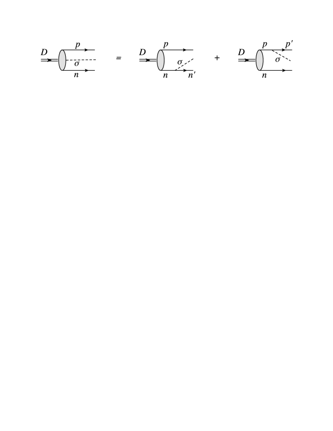
Figure D.1: Graphical representation of Eq. (D.1.1).

D.2 The electron-deuteron scattering problem

D.2.1 Matrix elements of the optical potential

The matrix elements of the third term in Eq. (8.4) of the optical have the following structure:

$$\langle\underline{v^{\prime}};\vec{\underline{k}}^{\prime}_{e},\underline{\mu}^{\prime}_{e};\vec{\underline{k}}^{\prime}_{D},\underline{\mu}^{\prime}_{D}|\hat{K}_{\gamma}(m-\hat{M}_{eD\gamma})^{-1}\hat{K}_{\sigma}(m-\hat{M}_{enp\sigma\gamma})^{-1}$$

$$\quad\times\hat{K}^{\dagger}_{\gamma}(m-\hat{M}_{enp\sigma})^{-1}\hat{K}_{\sigma}^{\dagger}|\underline{v};\vec{\underline{k}}_{e},\underline{\mu}_{e};\vec{\underline{k}}_{D},\underline{\mu}_{D}\rangle$$

$$\quad=\underline{v}_{0}\delta(\vec{\underline{v}}^{\prime}-\vec{\underline{v}})\frac{(2\pi)^{3}}{\sqrt{(\omega_{k^{\prime}_{e}}+\omega_{\underline{k}^{\prime}_{D}})^{3}(\omega_{k_{e}}+\omega_{\underline{k}_{D}})^{3}}}e\,\underbrace{\bar{u}_{\mu_{e}^{\prime}}(\vec{k}_{e}^{\prime})\gamma^{\mu}u_{\mu_{e}}(\vec{k}_{e})}_{j_{e}^{\mu}}$$

$$\quad\times|e|\;\left(\frac{1}{m-\omega_{k^{\prime}_{D}}-\omega_{k_{e}}-\omega_{k_{\gamma}}}\right)$$

$$\quad\times\sqrt{2\omega_{k_{D}}2\omega_{k^{\prime}_{D}}}\int d^{3}\tilde{k}^{\prime}_{p}\sqrt{\frac{\omega_{\tilde{k}^{\prime}_{n}}+\omega_{\tilde{k}^{\prime}_{p}}}{\omega_{k^{\prime}_{n}}+\omega_{k^{\prime}_{p}}}}\frac{1}{2\sqrt{\omega_{\tilde{k}^{\prime}_{n}}\omega_{\tilde{k}^{\prime}_{p}}}}$$

$$\quad\times\int d^{3}\tilde{k}_{p}\sqrt{\frac{\omega_{\tilde{k}_{n}}+\omega_{\tilde{k}_{p}}}{\omega_{k_{n}}+\omega_{k_{p}}}}\frac{1}{2\sqrt{\omega_{\tilde{k}_{n}}\omega_{\tilde{k}_{p}}}}\;\frac{1}{2\omega_{k_{\gamma}}}\frac{1}{2\omega_{k^{\prime\prime}_{p}}}\frac{1}{2\omega_{k_{\sigma}}}$$

$$\quad\times\left(\frac{1}{m-\omega_{k_{e}}-\omega_{k_{p}}-\omega_{k^{\prime}_{n}}-\omega_{k_{\sigma}}}\right)\left(\frac{g_{\mu\nu}}{m-\omega_{k_{e}}-\omega_{k^{\prime\prime}_{p}}-\omega_{k^{\prime}_{n}}-\omega_{k_{\sigma}}-\omega_{k_{\gamma}}}\right)$$

$$\quad\times\sum_{\mu_{p}^{\prime}\mu_{n}\mu_{p}}\sum_{\tilde{\mu}_{n}\tilde{\mu}_{p}\tilde{\mu}_{n}^{\prime}\tilde{\mu}_{p}^{\prime}}\bar{u}_{\mu^{\prime}_{p}}(\vec{k}^{\prime\prime}_{p})\Gamma^{\nu}u_{\mu_{p}}(\vec{k}_{p})g^{2}_{\sigma}\;\bar{u}_{\mu^{\prime}_{p}}(\vec{k}^{\prime}_{p})u_{\mu^{\prime}_{p}}(\vec{k}^{\prime\prime}_{p})\;\bar{u}_{\mu_{n}}(\vec{k}^{\prime}_{n})u_{\mu_{n}}(\vec{k}_{n})$$

$$\quad\times C^{1\mu_{D}^{\prime}}_{\frac{1}{2}\tilde{\mu}_{p}^{\prime}\frac{1}{2}\tilde{\mu}_{n}^{\prime}}\;D^{1/2}_{\tilde{\mu}_{p}^{\prime}\mu_{p}^{\prime}}\left[R_{W}^{-1}\left(\frac{\tilde{k}_{p}^{\prime}}{m_{p}},B_{c}\left(v_{np}\right)\right)\right]D^{1/2}_{\mu_{p}\tilde{\mu}_{p}}\left[R_{W}\left(\frac{\tilde{k}_{p}}{m_{p}},B_{c}\left(v_{np}\right)\right)\right]$$

$$\quad\times C^{1\mu_{D}}_{\frac{1}{2}\tilde{\mu}_{p}\frac{1}{2}\tilde{\mu}_{n}}D^{1/2}_{\tilde{\mu}_{n}^{\prime}\tilde{\mu}_{n}}\left[R_{W}^{-1}\left(\frac{\tilde{k}_{n}^{\prime}}{m_{n}},B_{c}\left(v_{np}^{\prime}\right)\right)R_{W}\left(\frac{\tilde{k}_{n}}{m_{n}},B_{c}\left(v_{np}\right)\right)\right]$$

$$\quad\times\text{u}^{*}_{D}(|\vec{\tilde{k}}_{p}^{\prime}|)Y^{*}_{00}(\hat{\vec{\tilde{k}}}_{p}^{\prime})\text{u}_{D}(|\vec{\tilde{k}}_{p}|)Y_{00}(\hat{\vec{\tilde{k}}}_{p})\;\;+\;\;(p\leftrightarrow n).$$ (D.5)

from which it is easy to identify the corresponding contribution to the deuteron current (cf. Chap. 3). In addition to the integration over $\tilde{k}^{\prime}_{p}$, a second integral appears, which runs over the intermediate state $\tilde{k}_{p}$ (in Sec. 8.4.2 $\tilde{k}_{p}^{\prime\prime}$ was chosen), and accounts for the momentum that is transferred by the $\sigma$-meson from one nucleon to the other. By a change of variables one can express this as an integration over this momentum transfer, which we call $\vec{\tilde{q}}$. The change requires some work, because $\vec{\tilde{k}}_{p}$ and $\vec{\tilde{q}}$ are defined in different reference frames. One has to transform $\vec{\tilde{k}}_{p}$ to $\vec{k}_{p}$ (see Eq. (B.4)), which is related to $\vec{\tilde{q}}$ by a simple translation:

$$\langle\underline{v^{\prime}};\vec{\underline{k}}^{\prime}_{e},\underline{\mu}^{\prime}_{e};\vec{\underline{k}}^{\prime}_{D},\underline{\mu}^{\prime}_{D}|\hat{K}_{\gamma}(m-\hat{M}_{eD\gamma})^{-1}\hat{K}_{\sigma}(m-\hat{M}_{enp\sigma\gamma})^{-1}$$

$$\quad\times\hat{K}^{\dagger}_{\gamma}(m-\hat{M}_{enp\sigma})^{-1}\hat{K}_{\sigma}^{\dagger}|\underline{v};\vec{\underline{k}}_{e},\underline{\mu}_{e};\vec{\underline{k}}_{D},\underline{\mu}_{D}\rangle$$

$$\quad=\underline{v}_{0}\delta(\vec{\underline{v}}^{\prime}-\vec{\underline{v}})\frac{(2\pi)^{3}}{\sqrt{(\omega_{k^{\prime}_{e}}+\omega_{\underline{k}^{\prime}_{D}})^{3}(\omega_{k_{e}}+\omega_{\underline{k}_{D}})^{3}}}\underbrace{e\bar{u}_{\mu_{e}^{\prime}}(\vec{k}_{e}^{\prime})\gamma^{\mu}u_{\mu_{e}}(\vec{k}_{e})}_{j_{e}^{\mu}}$$

$$\quad\times|e|\;\left(\frac{1}{m-\omega_{k^{\prime}_{D}}-\omega_{k_{e}}-\omega_{k_{\gamma}}}\right)$$

$$\quad\times\sqrt{2\omega_{k_{D}}2\omega_{k^{\prime}_{D}}}\int d^{3}\tilde{k}^{\prime}_{p}\sqrt{\frac{\omega_{\tilde{k}^{\prime}_{n}}+\omega_{\tilde{k}^{\prime}_{p}}}{\omega_{k^{\prime}_{n}}+\omega_{k^{\prime}_{p}}}}\frac{1}{2\sqrt{\omega_{\tilde{k}^{\prime}_{n}}\omega_{\tilde{k}^{\prime}_{p}}}}$$

$$\quad\times\int d^{3}\tilde{q}\frac{\sqrt{2\omega_{\tilde{k}_{p}}2\omega_{\tilde{k}_{n}}}}{2\omega_{k_{n}}2\omega_{k_{p}}}\sqrt{\frac{\omega_{k_{n}}+\omega_{k_{p}}}{\omega_{\tilde{k}_{n}}+\omega_{\tilde{k}_{p}}}}\frac{1}{2\omega_{k_{\gamma}}}\frac{1}{2\omega_{k^{\prime\prime}_{p}}}\frac{1}{2\omega_{k_{\sigma}}}$$

$$\quad\times\left(\frac{1}{m-\omega_{k_{e}}-\omega_{k_{p}}-\omega_{k^{\prime}_{n}}-\omega_{k_{\sigma}}}\right)\left(\frac{g_{\mu\nu}}{m-\omega_{k_{e}}-\omega_{k^{\prime\prime}_{p}}-\omega_{k^{\prime}_{n}}-\omega_{k_{\sigma}}-\omega_{k_{\gamma}}}\right)$$

$$\quad\times\sum_{\mu_{p}^{\prime}\mu_{n}\mu_{p}}\sum_{\tilde{\mu}_{n}\tilde{\mu}_{p}\tilde{\mu}_{n}^{\prime}\tilde{\mu}_{p}^{\prime}}\bar{u}_{\mu^{\prime}_{p}}(\vec{k}^{\prime\prime}_{p})\Gamma^{\nu}u_{\mu_{p}}(\vec{k}_{p})g^{2}_{\sigma}\;\bar{u}_{\mu^{\prime}_{p}}(\vec{k}^{\prime}_{p})u_{\mu^{\prime}_{p}}(\vec{k}^{\prime\prime}_{p})\;\bar{u}_{\mu_{n}}(\vec{k}^{\prime}_{n})u_{\mu_{n}}(\vec{k}_{n})$$

$$\quad\times C^{1\mu_{D}^{\prime}}_{\frac{1}{2}\tilde{\mu}_{p}^{\prime}\frac{1}{2}\tilde{\mu}_{n}^{\prime}}\;D^{1/2}_{\tilde{\mu}_{p}^{\prime}\mu_{p}^{\prime}}\left[R_{W}^{-1}\left(\frac{\tilde{k}_{p}^{\prime}}{m_{p}},B_{c}\left(v_{np}\right)\right)\right]D^{1/2}_{\mu_{p}\tilde{\mu}_{p}}\left[R_{W}\left(\frac{\tilde{k}_{p}}{m_{p}},B_{c}\left(v_{np}\right)\right)\right]$$

$$\quad\times C^{1\mu_{D}}_{\frac{1}{2}\tilde{\mu}_{p}\frac{1}{2}\tilde{\mu}_{n}}D^{1/2}_{\tilde{\mu}_{n}^{\prime}\tilde{\mu}_{n}}\left[R_{W}^{-1}\left(\frac{\tilde{k}_{n}^{\prime}}{m_{n}},B_{c}\left(v_{np}^{\prime}\right)\right)R_{W}\left(\frac{\tilde{k}_{n}}{m_{n}},B_{c}\left(v_{np}\right)\right)\right]$$

$$\quad\times\text{u}^{*}_{D}(|\vec{\tilde{k}}_{p}^{\prime}|)Y^{*}_{00}(\hat{\vec{\tilde{k}}}_{p}^{\prime})\text{u}_{D}(|\vec{\tilde{k}}_{p}|)Y_{00}(\hat{\vec{\tilde{k}}}_{p})\;\;+\;\;(p\leftrightarrow n).$$ (D.6)

It is now easy to identify the exchange current contribution, where the photon couples to the proton:

$$J_{p}^{\mu,\text{ex}}(\vec{k}_{D}^{\prime},\vec{k}_{D};\mu^{\prime}_{D},\mu_{D})=\sqrt{2\omega_{k_{D}}2\omega_{k^{\prime}_{D}}}\int d^{3}\tilde{k}^{\prime}_{p}\sqrt{\frac{\omega_{\tilde{k}^{\prime}_{n}}+\omega_{\tilde{k}^{\prime}_{p}}}{\omega_{k^{\prime}_{n}}+\omega_{k^{\prime}_{p}}}}\frac{1}{2\sqrt{\omega_{\tilde{k}^{\prime}_{n}}\omega_{\tilde{k}^{\prime}_{p}}}}$$

$$\quad\times\int d^{3}\tilde{q}\frac{\sqrt{2\omega_{\tilde{k}_{p}}2\omega_{\tilde{k}_{n}}}}{2\omega_{k_{n}}2\omega_{k_{p}}}\sqrt{\frac{\omega_{k_{n}}+\omega_{k_{p}}}{\omega_{\tilde{k}_{n}}+\omega_{\tilde{k}_{p}}}}\frac{1}{2\omega_{k_{\gamma}}}\frac{1}{2\omega_{k^{\prime\prime}_{p}}}\frac{1}{2\omega_{k_{\sigma}}}$$

$$\quad\times\left(\frac{1}{m-\omega_{k_{e}}-\omega_{k^{\prime\prime}_{p}}-\omega_{k^{\prime}_{n}}-\omega_{k_{\sigma}}-\omega_{k_{\gamma}}}\right)\left(\frac{1}{m-\omega_{k_{e}}-\omega_{k_{p}}-\omega_{k^{\prime}_{n}}-\omega_{k_{\sigma}}}\right)$$

$$\quad\times\sum_{\mu_{p}^{\prime}\mu_{n}\mu_{p}}\sum_{\tilde{\mu}_{n}\tilde{\mu}_{p}\tilde{\mu}_{n}^{\prime}\tilde{\mu}_{p}^{\prime}}\bar{u}_{\mu^{\prime}_{p}}(\vec{k}^{\prime\prime}_{p})\Gamma^{\nu}u_{\mu_{p}}(\vec{k}_{p})g^{2}_{\sigma}\;\bar{u}_{\mu^{\prime}_{p}}(\vec{k}^{\prime}_{p})u_{\mu^{\prime}_{p}}(\vec{k}^{\prime\prime}_{p})\;\bar{u}_{\mu_{n}}(\vec{k}^{\prime}_{n})u_{\mu_{n}}(\vec{k}_{n})$$

$$\quad\times C^{1\mu_{D}^{\prime}}_{\frac{1}{2}\tilde{\mu}_{p}^{\prime}\frac{1}{2}\tilde{\mu}_{n}^{\prime}}\;D^{1/2}_{\tilde{\mu}_{p}^{\prime}\mu_{p}^{\prime}}\left[R_{W}^{-1}\left(\frac{\tilde{k}_{p}^{\prime}}{m_{p}},B_{c}\left(v_{np}\right)\right)\right]D^{1/2}_{\mu_{p}\tilde{\mu}_{p}}\left[R_{W}\left(\frac{\tilde{k}_{p}}{m_{p}},B_{c}\left(v_{np}\right)\right)\right]$$

$$\quad\times C^{1\mu_{D}}_{\frac{1}{2}\tilde{\mu}_{p}\frac{1}{2}\tilde{\mu}_{n}}D^{1/2}_{\tilde{\mu}_{n}^{\prime}\tilde{\mu}_{n}}\left[R_{W}^{-1}\left(\frac{\tilde{k}_{n}^{\prime}}{m_{n}},B_{c}\left(v_{np}^{\prime}\right)\right)R_{W}\left(\frac{\tilde{k}_{n}}{m_{n}},B_{c}\left(v_{np}\right)\right)\right]$$

$$\quad\times\text{u}^{*}_{D}(|\vec{\tilde{k}}_{p}^{\prime}|)Y^{*}_{00}(\hat{\vec{\tilde{k}}}_{p}^{\prime})\text{u}_{D}(|\vec{\tilde{k}}_{p}|)Y_{00}(\hat{\vec{\tilde{k}}}_{p}).$$ (D.7)

The other terms in Eq. (8.4) can be treated in an analogous way.

D.2.2 The deuteron exchange currents in the infinite-momentum frame $\kappa_{D}\to\infty$

In the infinite-momentum frame the current matrix elements simplify further. The spinor product $\bar{u}_{\mu^{\prime}_{p}}(\vec{k}^{\prime\prime}_{p})\gamma^{\nu}u_{\mu_{p}}(\vec{k}_{p})$, e.g., becomes in this limit:

$$\bar{u}_{\frac{1}{2}}(\vec{k}^{\prime\prime}_{p})\gamma^{\mu}u_{\frac{1}{2}}(\vec{k}_{p})\rightarrow\left(\begin{array}[]{c}\kappa_{D}\frac{m^{\prime}_{np}+2\tilde{k}^{\prime}_{3}}{m^{\prime}_{np}}\\ 2\tilde{k}^{\prime}_{1}+\left(-\frac{1}{2}+\frac{\tilde{k}^{\prime}_{3}}{m^{\prime}_{np}}\right)\text{Q}-2\tilde{q}_{1}\\ 2\tilde{k}^{\prime}_{2}+i\text{Q}-2\tilde{q}_{2}\\ \kappa_{D}\frac{m^{\prime}_{np}+2\tilde{k}^{\prime}_{3}}{m^{\prime}_{np}}\end{array}\right);$$ (D.8)

$$\bar{u}_{\frac{1}{2}}(\vec{k}^{\prime\prime}_{p})\gamma^{\mu}u_{-\frac{1}{2}}(\vec{k}_{p})\rightarrow\left(\begin{array}[]{c}-\text{Q}\\ 0\\ 0\\ -\text{Q}\end{array}\right);\quad\bar{u}_{-\frac{1}{2}}(\vec{k}^{\prime\prime}_{p})\gamma^{\mu}u_{\frac{1}{2}}(\vec{k}_{p})\rightarrow\left(\begin{array}[]{c}\text{Q}\\ 0\\ 0\\ \text{Q}\end{array}\right);$$ (D.9)

$$\bar{u}_{-\frac{1}{2}}(\vec{k}^{\prime\prime}_{p})\gamma^{\mu}u_{-\frac{1}{2}}(\vec{k}_{p})\rightarrow\left(\begin{array}[]{c}\kappa_{D}\frac{m^{\prime}_{np}+2\tilde{k}^{\prime}_{3}}{m^{\prime}_{np}}\\ 2\tilde{k}^{\prime}_{1}+\left(-\frac{1}{2}+\frac{\tilde{k}^{\prime}_{3}}{m^{\prime}_{np}}\right)\text{Q}-2\tilde{q}_{1}\\ 2\tilde{k}^{\prime}_{2}-i\text{Q}-2\tilde{q}_{2}\\ \kappa_{D}\frac{m^{\prime}_{np}+2\tilde{k}^{\prime}_{3}}{m^{\prime}_{np}}\end{array}\right).$$ (D.10)

$$\omega_{k_{D}}\rightarrow\kappa_{D},\quad\omega_{k^{\prime}_{P}},\,\omega_{k^{\prime\prime}_{P}},\,\omega_{k_{P}}\rightarrow\kappa_{D}\left(\frac{1}{2}+\frac{\tilde{k}^{\prime}_{3}}{m^{\prime}_{12}}\right),\quad\omega_{k^{\prime}_{N}}\rightarrow\kappa_{D}\left(\frac{1}{2}-\frac{\tilde{k}^{\prime}_{3}}{m^{\prime}_{12}}\right)$$ (D.11)

And

$$\bar{u}_{\mu^{\prime}_{p}}(\vec{k}^{\prime}_{p})u_{\mu^{\prime}_{p}}(\vec{k}^{\prime\prime}_{p})\rightarrow\kappa_{D}\frac{m^{\prime}_{np}+2\tilde{k}^{\prime}_{3}}{m^{\prime}_{np}},\quad\bar{u}_{\mu_{n}}(\vec{k}^{\prime}_{n})u_{\mu_{n}}(\vec{k}_{n})\to\kappa_{D}\frac{m^{\prime}_{np}-2\tilde{k}^{\prime}_{3}}{m^{\prime}_{np}},$$

$$\frac{\sqrt{\omega_{k^{\prime}_{D}}\omega_{k_{D}}}}{2\omega_{k_{p}}}\to\frac{m_{pn}^{\prime}}{m_{pn}^{\prime}+2\tilde{k}_{3}}.$$ (D.12)

For point-like nucleons, i.e. $\Gamma_{p}^{\mu}=\gamma^{\mu}$ and $\Gamma_{n}^{\mu}=0$, Eq. (D.2.1) in the limit leads to:

$$J_{D}^{\mu,\text{ex}}(k^{\prime}_{D},\mu^{\prime}_{D};k_{D},\mu_{D})$$

$$\quad=\int d^{3}\tilde{k}^{\prime}_{n}\int d^{3}\tilde{q}\sqrt{\frac{m_{np}}{m^{\prime}_{np}}}g^{2}_{\sigma}\left(\frac{1}{\omega_{\sigma}}\right)^{2}\frac{1}{\text{Q}+\omega_{\sigma}}\frac{2m_{pn}^{\prime}}{m_{pn}^{\prime}+2\tilde{k}_{3}}$$

$$\quad\times\sum_{\mu_{p}^{\prime}}\sum_{\tilde{\mu}_{n}\tilde{\mu}_{p}\tilde{\mu}_{n}^{\prime}\tilde{\mu}_{p}^{\prime}}\text{u}^{*}_{D}(|\vec{\tilde{k}}_{p}^{\prime}|)Y^{*}_{00}(\hat{\vec{\tilde{k}}}_{p}^{\prime})\text{u}_{D}(|\vec{\tilde{k}}_{p}|)Y_{00}(\hat{\vec{\tilde{k}}}_{p})\;\,\bar{u}_{\mu_{p}^{\prime}}(\vec{k}^{\prime\prime}_{p})\gamma^{\mu}u_{\mu_{p}}(\vec{k}_{p})$$

$$\quad\times C^{1\mu_{D}^{\prime}}_{\frac{1}{2}\tilde{\mu}_{p}^{\prime}\frac{1}{2}\tilde{\mu}_{n}^{\prime}}\;D^{1/2}_{\tilde{\mu}_{p}^{\prime}\mu_{p}^{\prime}}\left[R_{W}^{-1}\left(\frac{\tilde{k}_{p}^{\prime}}{m_{p}},B_{c}\left(v_{np}\right)\right)R_{W}\left(\frac{\tilde{k}_{p}}{m_{p}},B_{c}\left(v_{np}\right)\right)\right]$$

$$\quad\times C^{1\mu_{D}}_{\frac{1}{2}\tilde{\mu}_{P}\frac{1}{2}\tilde{\mu}_{n}}D^{1/2}_{\tilde{\mu}_{n}^{\prime}\tilde{\mu}_{n}}\left[R_{W}^{-1}\left(\frac{\tilde{k}_{n}^{\prime}}{m_{n}},B_{c}\left(v_{np}^{\prime}\right)\right)R_{W}\left(\frac{\tilde{k}_{n}}{m_{n}},B_{c}\left(v_{np}\right)\right)\right].$$ (D.13)

Bibliography

- [1]
- [2] P. A. M. Dirac, Forms Of Relativistic Dynamics, Rev. Mod. Phys. 21 (1949) 392.
- [3] A. J. F. Siegert, Note on the interaction between nuclei and electromagnetic radiation, Phys. Rev. 52, 787 (1937).
- [4] B. D. Keister and W. N. Polyzou, Relativistic Hamiltonian dynamics in nuclear and particle physics, Adv. Nucl. Phys. 20, 225 (1991).
- [5] S. N. Sokolov, Relativistic Addition of Direct Interactions in the Point Form of Dynamics, Theor. Math. Phys. 36 (1979) 682 [Teor. Mat. Fiz. 36 (1978) 193].
- [6] F. Coester and W. N. Polyzou, Relativistic Quantum Mechanics Of Particles With Direct Interactions, Phys. Rev. D 26, 1348 (1982).
- [7] F. M. Lev, Exact construction of the electromagnetic current operator for relativistic composite systems, Annals Phys. 237 (1995) 355 [hep-ph/9403222].
- [8] N. Isgur and M. B. Wise, Weak Decays of Heavy Mesons in the Static Quark Approximation, Phys. Lett. B 232, 113 (1989).
- [9] N. Isgur and M. B. Wise, Weak Transition Form-factors Between Heavy Mesons, Phys. Lett. B 237, 527 (1990).
- [10] M. Neubert, Heavy quark symmetry, Phys. Rept. 245 (1994) 259 [hep-ph/9306320].
- [11] M. Gómez Rocha, F. J. Llanes-Estrada, D. Schütte and S. V. Chavez, Boost operators in Coulomb-gauge QCD: The Pion form factor and Fock expansions in phi radiative decays, Eur. J. Phys. A 44, 411 (2010) [arXiv:0910.1448 [hep-ph]].
- [12] S. J. Brodsky, H. -C. Pauli and S. S. Pinsky, Quantum chromodynamics and other field theories on the light cone, Phys. Rept. 301, 299 (1998) [hep-ph/9705477].
- [13] E. P. Biernat, W. H. Klink, W. Schweiger and S. Zelzer, Point-form quantum field theory. Annals Phys. 323, 1361 (2008) [arXiv:0708.1703 [nucl-th]].
- [14] E. P. Biernat, W. H. Klink and W. Schweiger, Point-Form Hamiltonian Dynamics and Applications. Few Body Syst. 49 (2011) 149 [arXiv:1008.0244 [nucl-th]].
- [15] B. Bakamjian and L. H. Thomas, Relativistic particle dynamics. 2. Phys. Rev. 92, 1300 (1953).
- [16] W. H. Klink, Relativistic simultaneously coupled multiparticle states. Phys. Rev. C 58, 3617 (1998).
- [17] W. H. Klink, Constructing point form mass operators from interaction Lagrangians. Nucl. Phys. A 716 (2003) 123 [nucl-th/0012031].
- [18] A. Krassnigg, W. Schweiger and W. H. Klink, Vector mesons in a relativistic point form approach. Phys. Rev. C 67 (2003) 064003 [nucl-th/0303063].
- [19] A. Krassnigg, Axial-vector mesons in a relativistic point-form approach. Phys. Rev. C 72 (2005) 028201 [nucl-th/0412017].
- [20] E. P. Biernat, W. Schweiger, K. Fuchsberger and W. H. Klink, Electromagnetic meson form factor from a relativistic coupled-channel approach. Phys. Rev. C 79, 055203 (2009) [arXiv:0902.2348 [nucl-th]].
- [21] E. P. Biernat, Electromagnetic Properties of Few-Body Systems Within a Point-Form Approach. PhD thesis, University of Graz (2011). [arXiv:1110.3180 [nucl-th]].
- [22] J. Carbonell, B. Desplanques, V. A. Karmanov and J. F. Mathiot, Explicitly covariant light front dynamics and relativistic few body systems. Phys. Rept. 300, 215 (1998) [nucl-th/9804029].
- [23] M. Gomez-Rocha and W. Schweiger, Electroweak form factors of heavy-light mesons: A relativistic point-form approach. Phys. Rev. D 86, 053010 (2012) [arXiv:1206.1257 [hep-ph]].
- [24] M. Gomez-Rocha and W. Schweiger, Form factors of heavy-light systems in point-form relativistic quantum mechanics: the Isgur-Wise function, Few Body Syst. 50, 227 (2011) [arXiv:1011.0547 [hep-ph]].
- [25] M. Gomez-Rocha, E. .P. Biernat and W. Schweiger, Form Factors of Few-Body Systems: Point Form Versus Front Form, Few Body Syst. 52, 397 (2012) [arXiv:1110.2355 [hep-ph]].
- [26] M. Gomez-Rocha and W. Schweiger, Electroweak hadron structure within a point-form approach, arXiv:1211.0868 [hep-ph].
- [27] B. D. Keister, Heavy quark symmetry and Dirac’s point form dynamics, Phys. Rev. D 46 (1992) 3188.
- [28] B. D. Keister, Relativity and the minimum slope of the Isgur-Wise function, hep-ph/9703310.
- [29] W. H. Klink, Point form relativistic quantum mechanics and electromagnetic form factors. Phys. Rev. C 58 (1998) 3587.
- [30] T. Melde, L. Canton, W. Plessas and R. F. Wagenbrunn, Spectator-model operators in point-form relativistic quantum mechanics. Eur. Phys. J. A 25 (2005) 97 [hep-ph/0411322].
- [31] W. Jaus, Semileptonic, radiative, and pionic decays of B, B* and D, D* mesons, Phys. Rev. D 53 (1996) 1349 [Erratum-ibid. D 54 (1996) 5904].
- [32] S. Simula, Calculation of the Isgur-Wise function from a light front constituent quark model, Phys. Lett. B 373, 193 (1996) [hep-ph/9601321].
- [33] N. B. Demchuk, I. L. Grach, I. M. Narodetski and S. Simula, Heavy to heavy and heavy to light weak decay form-factors in the light front approach: The Exclusive 0- to 0- case, Phys. Atom. Nucl. 59 (1996) 2152 [Yad. Fiz. 59N12 (1996) 2235] [hep-ph/9601369].
- [34] H. -Y. Cheng, C. -Y. Cheung and C. -W. Hwang, Mesonic form-factors and the Isgur-Wise function on the light front, Phys. Rev. D 55 (1997) 1559 [hep-ph/9607332].
- [35] H. -M. Choi and C. -R. Ji, Light-front quark model analysis of exclusive semileptonic heavy meson decays, Phys. Lett. B460, 461 (1999), hep-ph/9903496.
- [36] S. Simula, Comparison among Hamiltonian light front formalisms at and not equal to 0: Space - like elastic form-factors of pseudoscalar and vector mesons, Phys. Rev. C 66 (2002) 035201 [nucl-th/0204015].
- [37] B. L. G. Bakker, H. -M. Choi and C. -R. Ji, Transition form-factors between pseudoscalar and vector mesons in light front dynamics, Phys. Rev. D 67 (2003) 113007 [hep-ph/0303002].
- [38] D. Ebert, R. N. Faustov and V. O. Galkin, New analysis of semileptonic B decays in the relativistic quark model, Phys. Rev. D 75 (2007) 074008 [hep-ph/0611307].
- [39] V. Morenas, A. Le Yaouanc, L. Oliver, O. Pene and J. C. Raynal, Quantitative predictions for B semileptonic decays into D, D* and the orbitally excited D** in quark models a la Bakamjian-Thomas, Phys. Rev. D 56 (1997) 5668 [hep-ph/9706265].
- [40] A. Le Yaouanc, L. Oliver, O. Pene and J. C. Raynal, Covariant quark model of form-factors in the heavy mass limit, Phys. Lett. B 365 (1996) 319 [hep-ph/9507342].
- [41] Y. Huang and W. N. Polyzou, Exchange current contributions in null-plane quantum models of elastic electron deuteron scattering, Phys. Rev. C 80, 025503 (2009) [arXiv:0812.2180 [nucl-th]].
- [42] R. Kleinhappel and W. Schweiger, Hadron Resonances Within a Constituent-Quark Model, arXiv:1109.0127 [hep-ph].
- [43] D. Gromes, H. J. Rothe and B. Stech, Field quantization on the surface x-squared = constant, Nucl. Phys. B 75, 313 (1974).
- [44] S. Fubini, A. J. Hanson and R. Jackiw, New approach to field theory, Phys. Rev. D 7, 1732 (1973).
- [45] W. H. Klink, Point Form Quantum Field Theory on Velocity Grids. I. Bosonic Contractions, arXiv:0801.4039 [nucl-th].
- [46] M. Gomez-Rocha, Angular momentum decomposition of chiral multiplets in front form. Int. J. of Modern Physics A27 (2012) 1250163 [arXiv:1204.5362 [hep-th]].
- [47] E. P. Wigner, On Unitary Representations of the Inhomogeneous Lorentz Group, Annals Math. 40 (1939) 149 [Nucl. Phys. Proc. Suppl. 6 (1989) 9].
- [48] V. Bargmann, On Unitary ray representations of continuous groups, Annals Math. 59, 1 (1954).
- [49] L. L. Foldy, Relativistic particle systems with interactions, Phys. Rev. 122 (1961) 275.
- [50] M. Wirbel, B. Stech and M. Bauer, Exclusive Semileptonic Decays of Heavy Mesons, Z. Phys. C 29 (1985) 637.
- [51] N. Isgur and M. B. Wise, Relationship between form-factors in semileptonic anti-B and D decays and exclusive rare anti-B meson decays. Phys. Rev. D 42, 2388 (1990).
- [52] M. Neubert and V. Rieckert, New approach to the universal form-factors in decays of heavy mesons, Nucl. Phys. B 382 (1992) 97.
- [53] H. -Y. Cheng, C. -Y. Cheung, C. -W. Hwang and W. -M. Zhang, A Covariant light front model of heavy mesons within HQET, Phys. Rev. D 57 (1998) 5598 [hep-ph/9709412].
- [54] K. Abe et al. [Belle Collaboration], Measurement of B() and determination of , Phys. Lett. B 526, 258 (2002), hep-ex/0111082.
- [55] J. E. Bartelt et al. [CLEO Collaboration], Measurement of the lepton neutrino branching fractions and form-factor, Phys. Rev. Lett. 82, 3746 (1999), hep-ex/9811042.
- [56] B. Aubert et al. [BABAR Collaboration], Measurement of and the Form-Factor Slope in Decays in Events Tagged by a Fully Reconstructed Meson, Phys. Rev. Lett. 104, 011802 (2010), hep-ex/0904.4063.
- [57] J. Beringer et al. [Particle Data Group], Review of particle physics, Phys. Rev. D86, 010001 (2012).
- [58] K. Abe et al. [BELLE Collaboration], Determination of using the semileptonic decay , Phys. Lett. B 526 (2002) 247 [hep-ex/0111060].
- [59] N. E. Adam et al. [CLEO Collaboration], Determination of the decay width and , Phys. Rev. D 67 (2003) 032001 [hep-ex/0210040].
- [60] B. Aubert et al. [BABAR Collaboration], Measurement of the decay rate and , Phys. Rev. D 71 (2005) 051502 [hep-ex/0408027].
- [61] D. Asner et al. [Heavy Flavor Averaging Group Collaboration], Averages of b-hadron, c-hadron, and -lepton Properties, arXiv:1010.1589 [hep-ex].
- [62] C. -W. Hwang, Analyses of decay constants and light-cone distribution amplitudes for s-wave heavy meson, Phys. Rev. D 81 (2010) 114024 [arXiv:1003.0972 [hep-ph]].
- [63] J. D. Walecka, A Theory of highly condensed matter, Annals Phys. 83, 491 (1974).
- [64] B. Bakker and E. Biernat, Parameters in a Walecka-type model for the deuteron, PoS LC 2010 (2010) 015.
- [65] W. Pauli and F. Villars, On the Invariant regularization in relativistic quantum theory, Rev. Mod. Phys. 21 (1949) 434.
- [66] M. van Iersel, C. F. M. van der Burgh and B. L. G. Bakker, Techniques for solving bound state problems, hep-ph/0010243.
- [67] L. Y. Glozman and A. V. Nefediev, Chiral symmetry and the string description of excited hadrons, Phys. Rev. D 76, 096004 (2007) [arXiv:0704.2673 [hep-ph]].
- [68] L. Y. Glozman, Restoration of chiral and U(1)A symmetries in excited hadrons, Phys. Rept. 444, 1 (2007) [hep-ph/0701081], and references therein.
- [69] L. D. Landau and E. M. Lifshitz, Quantum Electrodynamics. Course of Theoretical Physics Vol. 4 (Pergamon Press, New York, 1982), Sec. 69, Problem 2.
- [70] L. Y. Glozman, C. B. Lang and M. Limmer, Angular momentum content of the rho-meson in lattice QCD, Phys. Rev. Lett. 103, 121601 (2009) [arXiv:0905.0811 [hep-lat]].
- [71] L. Y. Glozman and A. V. Nefediev, Chiral symmetry, the angular content of the vector current in QED and QCD, and the holographic description of hadrons, Phys. Rev. D 80, 057901 (2009) [arXiv:0904.3067 [hep-ph]].
- [72] M. Diehl, Generalized parton distributions, Phys. Rept. 388, 41 (2003) [arXiv:hep-ph/0307382].
- [73] D. E. Soper, Infinite-momentum helicity states, Phys. Rev. D 5 (1972) 1956.
- [74] G. P. Lepage and S. J. Brodsky, Exclusive Processes in Perturbative Quantum Chromodynamics, Phys. Rev. D 22 (1980) 2157.
- [75] L. D. Landau and E. M. Lifshitz, Quantum Mechanics: Non-Relativistic Theory. Course of Theoretical Physics Vol. 3 (Pergamon Press, 1977).
- [76] H. J. Melosh, Quarks: Currents and constituents, Phys. Rev. D 9, 1095 (1974).