New Image Statistics for Detecting Disturbed Galaxy Morphologies at High Redshift

Abstract

Testing theories of hierarchical structure formation requires estimating the distribution of galaxy morphologies and its change with redshift. One aspect of this investigation involves identifying galaxies with disturbed morphologies (e.g., merging galaxies). This is often done by summarizing galaxy images using, e.g., the $CAS$ and Gini-$M_{20}$ statistics of Conselice (2003) and Lotz et al. (2004), respectively, and associating particular statistic values with disturbance. We introduce three statistics that enhance detection of disturbed morphologies at high-redshift ($z\sim 2$): the multi-mode ($M$), intensity ($I$), and deviation ($D$) statistics. We show their effectiveness by training a machine-learning classifier, random forest, using 1,639 galaxies observed in the $H$-band by the Hubble Space Telescope WFC3, galaxies that had been previously classified by eye by the CANDELS collaboration (Grogin et al. 2011, Koekemoer et al. 2011). We find that the $MID$ statistics (and the $A$ statistic of Conselice 2003) are the most useful for identifying disturbed morphologies.

We also explore whether human annotators are useful for identifying disturbed morphologies. We demonstrate that they show limited ability to detect disturbance at high redshift, and that increasing their number beyond $\approx$10 does not provably yield better classification performance. We propose a simulation-based model-fitting algorithm that mitigates these issues by bypassing annotation.

1 Introduction

A thorough investigation of cosmological theories of hierarchical structure formation requires an accurate and precise estimate of the distribution of observed galaxy morphologies and how it varies as a function of redshift. One may attack this problem from a number of angles, including determining the galaxy (major and minor) merger fraction at a range of redshifts. Current estimates of the merger fraction at redshifts $z\leq$ 1.4 vary widely, from $\sim$ 0.01 to $\sim$ 0.1 (see, e.g., Lotz et al. 2011 and references therein), with quoted errors $\approx$0.01-0.03; at higher redshifts up to $z\sim$ 3, merger fraction estimates rise to as high as 0.4 (e.g., Conselice et al. 2003, Conselice, Rajgor, & Myers 2008, Bluck et al. 2012). Theory offers little guidance for resolving discrepancies among analyses: while the dark matter halo-halo merger fraction has been estimated consistently via simulations, uncertainty in the physical processes linking halos to underlying galaxies currently precludes consistent estimation of the galaxy merger fraction (e.g., Bertone & Conselice 2009, Jogee et al. 2009, Hopkins et al. 2010).

As stated in, e.g., Lotz et al. (2011), post-merger morphologies are sufficiently ambiguous that we cannot use local galaxies as an accurate tracer of the merger fraction and its evolution. Even if all merger events did result in the formation of spheroidal galaxies, the converse is not true: not all spheroidal galaxies arise from mergers. Thus to estimate the merger fraction and its evolution, we must seek out ongoing mergers themselves. High-redshift merger sample sizes range from the hundreds (e.g., Lotz et al. 2008, Jogee et al. 2009, Kartaltepe et al. 2010) to $\approx$1,600 (Bridge, Carlberg, & Sullivan 2010), a regime in which human-based analysis (i.e., annotation) is feasible. However, on-going surveys such as the Cosmic Assembly Near-IR Deep Extragalactic Legacy Survey (CANDELS; Grogin et al. 2011, Koekemoer et al. 2011) will increase the number of putative mergers to the tens of thousands.

One approach to inferring merger activity involves detecting disturbed morphologies within individual galaxies. Ideally, they would manifest themselves either as separate classes or as outliers within the evolving distribution of galaxy shapes, a distribution that we would estimate directly from an adequately large set of galaxy images. However, the direct use of galaxy images is both statistically and computationally intractable. Thus we instead transform inherently high-dimensional (i.e., multi-pixel) images into a lower-dimensional representations that retain important morphological information, and we use them to estimate discrete classes: early-type galaxies vs. late-type galaxies, mergers vs. non-mergers, etc.

Human annotators perform dimension reduction and discretization implicitly (e.g., Lintott et al. 2008, Bridge, Carlberg, & Sullivan 2010, Darg et al. 2010, Kartaltepe et al. 2010), but labeling galaxies is time consuming both in terms of infrastructure development and implementation. (Also, the inferential accuracy achieved by using many non-expert annotators$-$i.e., by crowdsourcing$-$versus that achieved by a smaller set of experts is an as-yet unresolved issue.) The main alternative to large-scale human labeling is to extract low-dimensional summary statistics (or features) from galaxy images, then to use the statistics and labels associated with a small subset of images to train a computer-based classifier. Of course, the effectiveness of this approach hinges upon how well we actually retain important morphological information when transforming image data, i.e., on whether we define an appropriate set of statistics.

There are a myriad of statistics that one may extract from image data. Common ones include the Sérsic index and bulge-to-disk ratio (found, e.g., using GALFIT; Peng et al. 2002). However, for our particular case of interest–detecting complex sub-structures in images of peculiar and irregular galaxies–statistics that do not require model fitting are clearly optimal. Such statistics include the concentration, asymmetry, and clumpiness ($CAS$) statistics (e.g., Bershady, Jangren, & Conselice 2000 and Conselice 2003, hereafter C03), and the Gini ($G$) and $M_{20}$ statistics (Abraham, van den Bergh, & Nair 2003 and Lotz, Primack, & Madau 2004, hereafter L04). Numerous authors apply these statistics; recent examples include Chen, Lowenthal, & Yun (2010), Kutdemir et al. (2010), Lotz et al. (2010a), Lotz et al. (2010b), Conselice et al. (2011), Holwerda et al. (2011), Mendez et al. (2011), and Hoyos et al. (2012).

Given this context, there are three outstanding issues in galaxy morphology analysis that we address in this work.

• The efficacy of the $CAS$ and $GM_{20}$ statistics for detecting disturbed morphologies degrades as galaxy signal-to-noise and size decrease, i.e., as redshift increases (see, e.g., Figures 9 and 19 of Conselice, Bershady, & Jangren 2000, Figures 5-6 of L04, and Lisker 2008). In §2, we define three new statistics (which we dub the $MID$ statistics) that improve our ability to collectively detect peculiar and irregular galaxies (which we dub non-regulars) as well as to detect merging systems themselves. In §4, we apply these statistics to the analysis of 1639 high-redshift ($z\sim$ 2) galaxies in the GOODS-South Early Release Science field (Windhorst et al. 2011), observed in the near-infrared regime by the Wide-Field Camera 3 (WFC3) on-board the Hubble Space Telescope (HST).

• Authors generally apply the $CAS$ and $GM_{20}$ in a non-optimal manner, by projecting high-dimensional spaces containing values for each observed galaxy down to two-dimensional planes (e.g., $G$-$M_{20}$) and delineating classes by eye. In §3, we introduce the use of random forest, a machine learning-based classifier that one can directly apply to high-dimensional spaces of image statistics, to morphological analysis. Ultimately, for analysis of large datasets, one would use random forest to to train a classifier on a small subset of labeled galaxies, then apply it to the unlabeled galaxies.

• What is contribution of annotators and their biases to the overall error budget in morphological analyses? For instance, the fact that widely varying merger fraction estimates are generally associated with small error bars indicates clearly the presence of (as yet unmodeled) systematic errors. These errors (such as that associated with the inability of various authors to agree on what defines a merger) may ultimately doom those morphological analyses in which humans play a role. In §5, we first examine whether it is always beneficial to have more annotators look at each galaxy image, then ask whether it even necessary to invoke annotation if our ultimate goal is to constrain models of hierarchical structure formation.

In §6, we summarize our results and discuss future research directions.

2 The MID statistics

Let $f_{i,j}$ denote the observed flux at pixel $(i,j)$ of a given image that has $n=n_{x}\times n_{y}$ pixels overall. We assume that associated with the image is a segmentation map that defines the extent of the object of interest, such as is output by, e.g., the source detection package Sextractor (Bertin & Arnouts 1996).

2.1 M(ulti-mode) statistic

Let $q_{l}$ denote an intensity quantile; for instance, $q_{0.8}$ denotes an intensity value such that 80 percent of the pixel intensities inside the segmentation map are smaller than this value. For a given value of $l$, we examine image pixels and define a new image

$$g_{i,j}=\left\{\begin{array}[]{cl}1&f_{i,j}\geq q_{l}\\ 0&\mbox{otherwise}\end{array}\right.\,.$$ (3)

This image will be mostly 0, with $m$ groups of contiguous pixels of value 1 where the galaxy intensity is largest. We determine the number of pixels $A_{l,m}$ in each group, and order them in descending order (i.e., $A_{l,(1)}$ is the largest group of contiguous pixels for quantile $l$, $A_{l,(2)}$ is the second-largest group, etc.). We define the area ratio for each quantile as

$$R_{l}=\frac{A_{l,(2)}}{A_{l,(1)}}A_{l,(2)}\,,$$ (4)

This statistic is suited for detecting double nuclei within the segmentation map, as the ratio $A_{l,(2)}/A_{l,(1)}$ tends towards 1 if double nuclei are present, and towards 0 if not. Because this ratio is sensitive to noise, we multiply it by $A_{l,(2)}$, which tends towards 0 if the second-largest group is a manifestation of noise. The multi-mode statistic is the maximum $R_{l}$ value, i.e.,

$$M=\max_{l}\,R_{l}\,.$$ (5)

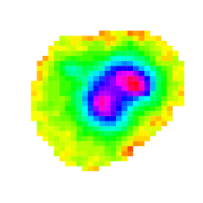
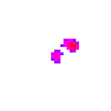
Figure 1: Example of pixel grouping for computing the multi-mode ($M$) statistic. To the left we display the $H$-band pixel intensities for an example of a merger galaxy (see Figure 3), while to the right we show only those pixels associated with the largest 5.8% of the sorted intensity values. The two pixel regions have areas $A_{(1)}=21$ and $A_{(2)}=14$, so that $R_{0.942}=(14/21)*14=9.33$. The $M$ statistic is the largest of the $R$ values computed for a sufficiently large number of threshold percentiles.

2.2 I(ntensity) statistic

The $M$ statistic is a function of the footprint areas of non-contiguous groups of image pixels, but does not take into account pixel intensities. To complement it, we define a similar statistic, the intensity or $I$ statistic. A readily apparent, simple definition of this statistic is the ratio of the sums of intensities in the two pixel groups used to compute $M$. However, this is not optimal, as in any given image it is possible, e.g., that a high-intensity pixel group with small footprint may not enter into the computation of $M$ in the first place.

There are myriad ways in which one can define pixel groups over which to sum intensities. In this work, we utilize a two-pronged approach. First, we smooth the data in each image with a symmetric bivariate Gaussian kernel, selecting the optimal width $\sigma$ by maximizing the relative importance of the $I$ statistic in correctly identifying morphologies (i.e., how well we can differentiate classes using the $I$ statistic alone, relative to how well we can differentiate classes by using other statistics by themselves; see §3.3). Then we define groups using maximum gradient paths. For each pixel in the smoothed image, we examine the surrounding eight pixels and move to the one for which the increase in intensity is maximized, repeating the process until we reach a local maximum. A single group consists of all pixels linked to a particular local maximum. (See Figure 2.) Once we define all pixel groups, we sum the intensities within each and sort the summed intensities in descending order: $I_{(1)}$, $I_{(2)}$,… The intensity statistic is then

$$I=\frac{I_{(2)}}{I_{(1)}}\,.$$ (6)

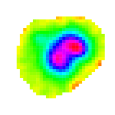
Figure 2: Example of pixel grouping for computing the intensity ($I$) statistic. To the left we display pixel intensities for an example of a merger galaxy (see Figure 3). These data are smoothed using a symmetric Gaussian kernel of width $\sigma$ = 1 pixel, a sufficiently small scale to remove local intensity maxima caused by noise without removing local maxima intrinsic to the galaxy itself. (See the text for details on how we select the appropriate smoothing scale $\sigma$.) To the right we display pixel regions associated with each local intensity maximum remaining after smoothing. Pixel intensities are summed within each region, with the intensity statistic then being the ratio of the second-largest to largest sum. In this example, the statistic is $I$ = 0.935.

2.3 D(eviation) statistic

Galaxies that are clearly irregular or peculiar will exhibit marked deviations from elliptical symmetry. A simple measure quantifying this deviation is the distance from a galaxy’s intensity centroid to the local maximum associated with $I_{(1)}$, the pixel group with maximum summed intensity. We expect this quantity to cluster near zero for spheroidal and disk galaxies. For those disk galaxies with well-defined bars and/or spiral arms, we would still expect near-zero values, as between the bulge and generally expected structure symmetry, both the intensity centroid and the maximum associated with $I_{(1)}$ should lie at the galaxy’s core.

We define the intensity centroid of a galaxy as

$$(x_{\rm cen},y_{\rm cen})=\left(\frac{1}{n_{\rm seg}}\sum_{i}\sum_{j}if_{i,j},\frac{1}{n_{\rm seg}}\sum_{i}\sum_{j}jf_{i,j}\right)\,.$$

with the summation being over all $n_{\rm seg}$ pixels with the segmentation map. The distance from $(x_{\rm cen},y_{\rm cen})$ to the maximum associated with $I_{(1)}$ will be affected by the absolute size of the galaxy; it generally will be larger for, e.g., galaxies at lower redshifts. Thus we normalize the distance using an approximate galaxy “radius,” $\sqrt{n_{\rm seg}/\pi}$. The deviation statistic is then

$$D=\sqrt{\frac{\pi}{n_{\rm seg}}}\sqrt{(x_{\rm cen}-x_{I_{(1)}})^{2}+(y_{\rm cen}-y_{I_{(1)}})^{2}}\,.$$ (7)

We have designed the $D$ statistic to capture evidence of galaxy asymmetry. It is thus complimentary to the $A$ statistic defined in C03, which is computed by rotating an image by 180^∘, taking the absolute difference between rotated and unrotated images, normalizing by the value of the unrotated image, and summing the resulting values pixel-by-pixel. In §4 we compute both $A$ and $D$ for a sample of high-redshift galaxies and show that while there is a large positive sample correlation coefficient between the two statistics, there are many instances where $D$ captures stronger evidence of asymmetry than $A$, and vice-versa, demonstrating that $D$ and $A$ are not simply redundant.

3 Statistical analysis: random forest

We use the $MID$ (and other) statistics to populate an $p$-dimensional space, where each axis represents the values of the $i^{\rm th}$ statistic and each data point represents one galaxy. Ideally, in this space, the set of points representing, e.g., visually identified mergers is offset from those representing non-mergers. To determine an optimal boundary between these point sets directly in the $n$-dimensional space, we apply machine-learning based methods of regression and classification. To ensure robust results, it is good practice to apply a number of methods to see if any one or more provide significantly better results. In our analysis of HST data in §4, we tested four algorithms: random forest, lasso regression, support vector machines, and principal components regression (for details on these, see, e.g., HFT09). We found that the results of applying each were similar: in the vast majority of cases, galaxies were either classified correctly or incorrectly by all four algorithms. Thus in this work we describe only the conceptually simplest of the four algorithms, random forest (Breiman 2001). For an example of an analysis code that uses random forest, see Appendix A.

3.1 Random Forest Regression

The first step in applying random forest is a regression step: we randomly sample 50% of the galaxies (i.e., populate a training set) and regress the fraction of annotators, $Y_{i}\in[0,1]$, who view galaxy $i$ as a non-regular/merger upon that galaxy’s set of image statistics. In random forest, bootstrap samples of the training set are used to grow $t$ trees (e.g., $t$ = 500), each of which has $n$ nodes (e.g., $n$ = 8). At each node in each tree, a random subset of size $m$ of the statistics is chosen (e.g., $C$, $M_{20}$, and $I$ may be chosen from the full set of statistics). The best split of the data along each of the $m$ axes is determined, with the one overall best split retained. This process is repeated for each node and each tree; subsequently the training data are pushed down each tree to determine $t$ class predictions for each galaxy (i.e., to generate a set of $t$ numbers for each galaxy, all of which are either 0 or 1). Let $s_{i}\in[0,t]$ equal the sum of the class predictions for galaxy $i$; then the random forest prediction for the galaxy’s classification is ${\hat{Y}}_{i}=s_{i}/t$.

While fitting the training data, random forest keeps track of all $t$ trees it creates, i.e., all of the data splits it performs. Thus any new datum (from the remaining 50% of the data, or the test set) may be “pushed” down these trees, resulting again in $t$ class predictions and thus a predicted response (or dependent) variable ${\hat{Y}}_{i}=s_{i}/t$.

3.2 Random Forest Classification

Once we predict response variables for the test set galaxies, we perform the second step of random forest, the classification step. First, the continuous fractions $Y_{i}$ associated with the test set galaxies are mapped to $Y_{{\rm class},i}=0$ if $Y_{i}<0.5$ and $Y_{{\rm class},i}=1$ if $Y_{i}>0.5$. (Ties are broken by randomly assigning galaxies to classes.) Then the predicted responses for the test set galaxies, ${\hat{Y}}_{i}$, are also mapped to discrete classes. Intuitively, one might expect the splitting point between predicted classes, $c$, to be 0.5. However, because the proportions of regular and non-regular galaxies in the training set are unequal, as are the proportions of non-merger and merger galaxies, regression will be biased towards fitting the galaxies of the more numerous type well. For instance, regular galaxies outnumber non-regular galaxies by approximately three-to-one, so a priori we expect the best value for $c$ to be around 1/(3+1) = 0.25. To determine $c$, we select a sequence of values $\{c_{1},c_{2},\cdots,c_{n}\}\in[0,1]$, and for each $c_{j}$ we map the predicted responses to two classes, e.g., we call all galaxies with predicted responses $\hat{Y}_{i}>c_{j}$ non-regulars/mergers. Call this classifying function $h(X,c_{j})$, where $X$ is the set of observed statistics. Our estimate of risk as a function of $c_{j}$ is the the overall proportion of misclassified galaxies:

$$\hat{R}_{j} = \hat{P}[h(X,c_{j})=0|Y=1]+\hat{P}[h(X,c_{j})=1|Y=0]$$

where $\hat{P}[h(X,c_{j})=0|Y=1]$ and $\hat{P}[h(X,c_{j})=1|Y=0]$ are the estimated probabilities of misclassifying a non-regular/merger and a regular/non-merger, respectively. We seek the minimum value for this estimate of risk. We smooth the discrete function $\hat{R}_{j}=f(c_{j})$ with a Gaussian profile of width 0.05, and choose as our final value of $\hat{c}$ that value for which the smoothed function $\hat{R}(c)$ is minimized.

3.3 Measures of Classifier Performance

Table 1: Confusion Matrix: Definitions

	Predicted	Predicted
	Regular/	Non-Regular/
	Non-Merger	Merger
Actual	TN	FP
Regular/	(true negatives)	(false positives)
Non-Merger
Actual	FN	TP
Non-Regular/	(false negatives)	(true positives)
Merger

We use a number of measures of classifier performance.

• Sensitivity. The proportion of non-regular/merger galaxies that are correctly classified: $TP/(TP+FN)$. (This is also dubbed completeness.)

• Specificity. The proportion of regular/non-merger galaxies that are correctly classified: $TN/(TN+FP)$.

• Estimated Risk. The sum of 1 $-$ sensitivity and 1 $-$ specificity.

• Total Error. The proportion of misclassified galaxies.

• Positive Predictive Value (PPV). The proportion of actual non-regular/merger galaxies among those predicted to be non-regulars or mergers: $TP/(TP+FP)$. (This is also dubbed purity.)

• Negative Predictive Value (NPV). The proportion of actual regular/non-merger galaxies among those predicted to be regulars or non-mergers: $TN/(TN+FN)$.

We define the symbols used above in Table 1.

Random forest assesses the efficacy of each statistic for disambiguating classes by computing Gini importance scores for each (see, e.g., Chapter 9 of HFT09; note that the Gini importance score differs from the Gini statistic $G$). At any given node of any tree, the $n$ samples to be split belong to two classes (e.g., merger/non-merger), with proportions $p_{1}=n_{1}/n$ and $p_{2}=n_{2}/n$. A metric of class impurity at this node is $i=1-p_{1}^{2}-p_{2}^{2}$. The samples are then split along the axis associated with one chosen image statistic, with proportions $p_{l}=n_{l}/n$ and $p_{r}=n_{r}/n$ being assigned to two daughter nodes. New values of the impurity metric are computed at each daughter node; call these values $i_{l}$ and $i_{r}$. The reduction in impurity achieved by splitting the data is $\Delta i=i-p_{l}i_{l}-p_{r}i_{r}$. Each value of $\Delta i$ is associated with one image statistic; the average of the $\Delta i$’s for each image statistic over all nodes and all trees is the Gini importance score.

Note that in this work, we are not as concerned with the absolute importance score of each statistic (which is not readily interpretable) as we are with relative scores derived by, e.g., dividing importance scores by the maximum observed importance score value. Relative scores are sufficient to allow us to rank the image statistics in order of how useful they are by themselves in classification. They also allow us to reduce the dimensionality of our statistic space, if necessary, by eliminating those that are not as useful for disambiguating classes. This point is not important in the context of implementing random forest$-$the random forest algorithm is computationally efficient even when presented with very high dimensional spaces of statistics$-$but does become important if we are to implement density-estimation-based analysis schemes like that discussed in §5.3.

4 Application to HST images of GOODS-S galaxies

We demonstrate the efficacy of the $MID$ statistics for detecting non-regular and merging galaxies by analyzing $H$- and $J$-band Hubble Space Telescope WFC3 images of the northernmost part of the Great Observatories Origins Deep Survey (GOODS) South field (the Early Release Science fields; see Windhorst et al. 2011 and references therein). These images have been analyzed by members of the Cosmic Assembly Near-IR Deep Extragalactic Legacy Survey (CANDELS; Grogin et al. 2011, Koekemoer et al. 2011) team. They ran SExtractor to extract a catalog of 6178 putative sources and associated segmentation maps in the $H$-band images, with the input parameters set so as to optimize the detection and deblending of galaxies at $z\sim 2$ (D. Kocevski, private communication). Subsequent visual morphological evaluation of these sources by, typically, three or four CANDELS team members yielded a set of 1639 galaxies with isophotal magnitudes $H<25$ (Kartaltepe et al. 2012, in preparation). In Figure 3 we show an example of one galaxy from the catalog that annotators identified as undergoing a merger.

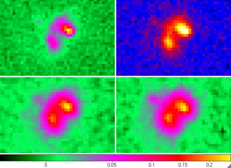
Figure 3: Example of a galaxy identified as a merging galaxy by CANDELS team annotators. Top Left and Right: HST ACS $V$- and $z$-band images, respectively. Bottom Left and Right: HST WFC3 $J$- and $H$-band images, respectively. Note the clear presence of two nuclei in the $J$-band image.

CANDELS-team labels are based primarily on $H$-band images, with data in the other three bands used to inform labeling. An annotator may first choose one (or more) “main” morphological class(es) (e.g., spheroid, disk, irregular), then indicate whether the galaxy is in the process of merging (or interacting within or beyond the segmentation map). Determining the fraction of annotators identifying a particular galaxy as a merger is straightforward. However, because individual annotators could register more than one vote, and because only the final vote totals are available, it is impossible to determine how many annotators labeled any one galaxy both as irregular and a merger as opposed to selecting only one of the two (as well as to determine the number of annotators, period). We thus estimate the fraction of votes for non-regularity, $f=V_{\ast}/V$, where $V$ is the total number of votes, by defining $V_{\ast}$ as

$$V_{\ast}\equiv{\rm mean}(V_{\ast}^{\rm low},V_{\ast}^{\rm high})\,,$$

with

$$V_{\ast}^{\rm low} = {\rm max}\{{\rm votes\,for\,irregular,votes\,for\,merger}\}$$

and

$$V_{\ast}^{\rm high} = {\rm max}\{{\rm votes\,for\,irregular\,+\,votes\,for\,merger},V\}$$

representing lower and upper bounds on the number of annotators that voted for merger or irregular.

4.1 Base Analysis: H-band Data

In our base analysis, we apply random forest regression and classification to detect non-regulars and mergers within a labeled set of 1639 galaxies observed in the $H$-band.For each galaxy, we have as the predictor (or independent) variables

• the $MID$ statistics, which we compute using postage stamp images (generally 84 $\times$ 84 pixels) and a segmentation map; and

• the $CAS$ (a la C03) and $GM_{20}$ statistics (a la L04), as provided by the CANDELS collaboration.

Recall that prior to computing the $I$ and $D$ statistics, we smooth the data with a symmetric Gaussian kernel of width $\sigma$ to mitigate the effect of local intensity maxima caused by noise (see §2.2). We choose $\sigma$ by maximizing the importance of the $I$ statistic; here, $\sigma$ = 1 pixel for both the non-regular and merger analyses. The continuous response variable $Y\in[0,1]$ is

• $f=V_{\ast}/V$, as estimated from visual annotations by members of the CANDELS collaboration. The numbers of galaxies with vote fractions favoring non-regularity of $f>0.5$ and $f=0.5$ are 337 and 163, respectively; the analogous numbers for the merger analysis are 109 and 71.

In Figure 4, we display the relative importance of each of the $CAS$-$GM_{20}$-$MID$ statistics for detecting non-regulars (x-axis) and mergers (y-axis). These values are normalized such that the value of the most important statistic, the $I$ statistic in the regular/non-regular analysis, is one. (To interpret relative importance, note for instance that the $M$ statistic by itself performs about half as well at differentiating regulars from non-regulars as the $I$ statistic by itself. This implies that there is greater separation between the distributions of $I$ statistics observed for regulars and for non-regulars than there is for the analogous $M$ statistic distributions. See Figure 5.) The error bars in Figure 4 represent the standard deviations of the populations from which we sample importance values, and are estimated by running random forest 1,000 times, i.e., by randomly dividing the 1,639 galaxies into training and test sets 1,000 times and recording variable importance and measures of classifier performance each time. Several conclusions are readily apparent when we examine Figure 4: (a) the $I$ statistic is the most important for detecting both non-regulars and mergers; (b) as expected, the $M$ statistic outperforms the $D$ statistic in merger detection, and vice-versa for detection of non-regulars; and (c) the $MID$ statistics, along with the $A$ (asymmetry) statistic of C03, are far more important for identifying non-regulars/mergers than the other statistics we examine.

Figure 5 displays projections of the four-dimensional space of image statistics defined by the $MID$ and $A$ statistics and indicates the distributions of these statistics for mergers (green points), non-regulars that are not mergers (blue points), and regulars (red contour lines). The reader should intuitively picture classification via random forest as placing vertical and horizontal lines on these plots so as to maximize the proportion of, e.g., non-regulars on one side and the proportion of regulars on the other. Given this intuitive picture, the relative efficacy of, e.g., the $I$ statistic with respect to the other statistics is clearly evident.Also evident from Figure 5 is our relative inability to separate mergers and irregular galaxies using $MID$ and $A$ alone. Further work is needed to develop image statistics that will optimize merger-irregular class separation.

The results in Figure 4 were generated by analyzing the entire eight-dimensional space of image statistics with random forest. Given that the number of possibly useful statistics will only increase in the future, it is important to determine we can disregard any of our current statistics with little, if any, loss in classifier performance. (This is not a trivial issue, as we discuss in §5.3: the number of statistics we incorporate may limit future analyses.) To that end, we define and analyze three reduced statistic sets for both the regular/non-regular case ($ID$,$A$-$ID$,$A$-$MID$) and the non-merger/merger case ($MI$,$A$-$MI$,$A$-$MID$), based on rankings of relative statistic importance.

See Tables LABEL:tab:HRNR and LABEL:tab:HNMM. The interpretation of these tables depends on the performance metric one prefers: e.g., sensitivity (or catalog completeness), estimated risk, or PPV (or catalog purity), etc. If we assume that one would wish to strike a balance between all three of these measures, we find that the reduced statistic set $A$-$ID$ is sufficient for disambiguating regulars from non-regulars, while one requires the additional information carried by the full set of statistics to disambiguate mergers from non-mergers.

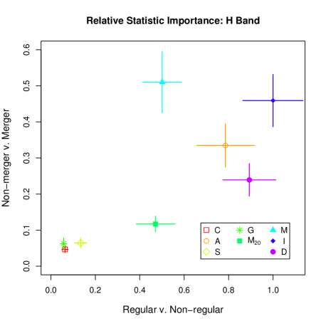
Figure 4: Relative importance of statistics in differentiating between regular and non-regular galaxies (x-axis) and non-merger and merging galaxies (y-axis) in CANDELS-team-processed $H$-band data, as output by the random forest classification algorithm. The values of all data points have been normalized by the value of the $I$ statistic for the regular/non-regular analysis. See §3.3 for the definition of statistic importance, and §4.1 for practical interpretation of the results. The error bars indicate sample standard deviation given 1,000 separate runs of random forest, and thus are not measures of the standard error of the mean; the 1$\sigma$ uncertainties in the means are given by shrinking the error bars by a factor of $\sqrt{1000}$ = 31.62.

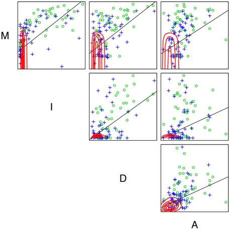
Figure 5: Scatter plots of the $MID$ and $A$ statistics as computed for CANDELS-team-processed $H$-band images. Green circles represent galaxies visually identified as mergers and blue crosses represent non-regulars that are not also mergers. The red lines are contours indicating the density of regular galaxies. The non-zero slopes of the black line, the best-fit linear regression functions, indicates the expected positive correlations between each of these statistics. Note that for increased clarity, only 100 randomly selected non-regulars/mergers are displayed.

Table 2: Classifier Performance $\times$ 10⁴ $-$ $H$-band/Non-Regular

	$ID$	$A$-$ID$	$A$-$MID$	Full
sens	7562 $\pm$ 14	7907 $\pm$ 11	7873 $\pm$ 11	7874 $\pm$ 13
spec	8071 $\pm$ 13	8187 $\pm$ 7	8136 $\pm$ 7	8181 $\pm$ 10
risk	4366 $\pm$ 8	3906 $\pm$ 8	3991 $\pm$ 8	3945 $\pm$ 8
toterr	2056 $\pm$ 7	1883 $\pm$ 4	1930 $\pm$ 4	1897 $\pm$ 5
PPV	5712 $\pm$ 13	5943 $\pm$ 9	5865 $\pm$ 9	5977 $\pm$ 11
NPV	9089 $\pm$ 4	9215 $\pm$ 4	9199 $\pm$ 4	9194 $\pm$ 4

This table displays sample mean plus/minus 1$\sigma$ standard error, each multipled by 10⁴.

Table 3: Classifier Performance $\times$ 10⁴ $-$ $H$-band/Merger

	$MI$	$A$-$MI$	$A$-$MID$	Full
sens	6917 $\pm$ 22	7520 $\pm$ 22	7790 $\pm$ 17	7816 $\pm$ 17
spec	8683 $\pm$ 14	8546 $\pm$ 15	8564 $\pm$ 9	8591 $\pm$ 8
risk	4400 $\pm$ 13	3934 $\pm$ 13	3646 $\pm$ 13	3594 $\pm$ 13
toterr	1477 $\pm$ 12	1547 $\pm$ 12	1506 $\pm$ 7	1480 $\pm$ 6
PPV	3562 $\pm$ 20	3525 $\pm$ 20	3541 $\pm$ 13	3603 $\pm$ 13
NPV	9662 $\pm$ 2	9723 $\pm$ 2	9752 $\pm$ 2	9753 $\pm$ 2

This table displays sample mean plus/minus 1$\sigma$ standard error, each multipled by 10⁴.

4.2 Effect of changing the observation wavelength: J-band data

Recall that CANDELS team labels are based primarily on how galaxies appear in the $H$ band. However, in order to, e.g., differentiate true mergers from galaxies exhibiting disk instabilities, we will need to extend the application of our statistics to other wavelength regimes. This extension is the subject of a future work; here, we make a preliminary assessment of the robustness of the $MID$ statistics as a function of wavelength by applying them to the $J$-band images associated with our galaxy sample.

In Figure 6, we display the relative importance of the $CAS$-$GM_{20}$-$MID$ statistics for the detection of non-regulars (x-axis) and mergers (y-axis) when we analyze $J$-band rather than $H$-band images. (For these data, the smoothing scales were 0.75 and 1.4 pixels for the non-regular and merger analyses, respectively.) The conclusions that we draw from this figure and from Table LABEL:tab:J are similar to those drawn from Figure 4 and Tables LABEL:tab:HRNR and LABEL:tab:HNMM: the $MID$ statistics are robust against changes in observation wavelength.

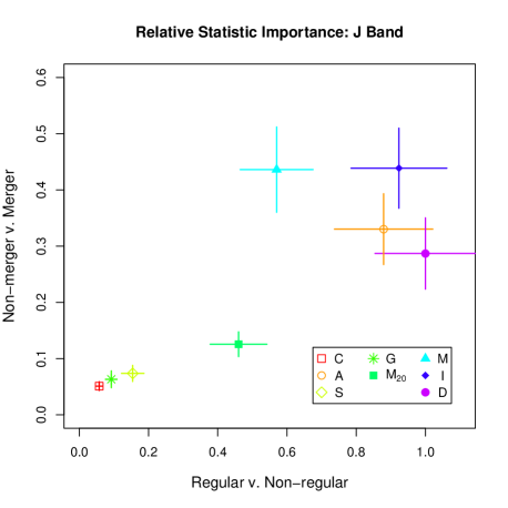
Figure 6: Same as Figure 4, but for $J$-band data. The similarity of this figure to Figure 4 indicates the robustness of the $MID$ statistics across wavelength regimes.

Table 4: Classifier Performance $\times$ 10⁴ $-$ $J$-band

	Regular/Non-Regular	Non-Merger/Merger
sens	7747 $\pm$ 14	7594 $\pm$ 18
spec	8124 $\pm$ 11	8295 $\pm$ 9
risk	4129 $\pm$ 8	4112 $\pm$ 14
toterr	1973 $\pm$ 6	1770 $\pm$ 7
PPV	5947 $\pm$ 12	3143 $\pm$ 11
NPV	9119 $\pm$ 4	9715 $\pm$ 2

This table displays sample mean plus/minus 1$\sigma$ standard error, each multipled by 10⁴.

4.3 Effect of changing the segmentation algorithm

The SExtractor segmentation maps used in the analysis of §4.1 associate image pixels with galaxies using an absolute surface brightness threshold, such that the fraction of galaxy flux within the map aperture varies with galaxy brightness. This can introduce redshift-dependent biases into analyses due to surface brightness dimming. We verify that our results from §4.1 are robust to segmentation algorithm by reanalyzing the data using an algorithm based on that of L04, who compute a Petrosian radius for each galaxy, i.e., the radius at which the mean surface brightness within an elliptical annulus is a fraction $\eta$ (e.g., 0.2) of the mean brightness within that radius. The assumption of ellipticity will bias the construction of maps for disturbed galaxies, so we generalize the algorithm by using intensity quantiles. We define a grid of quantile values and begin with the largest value, determining which pixels have intensities greater than this value and summing their intensities. We then systematically decrease the quantile value until the mean surface brightness of newly added pixels is a fraction $\eta$ of the mean brightness of all pixels with intensities above the quantile value. Because segmentation maps produced by this algorithm are based on relative changes in surface brightness, these maps are nominally redshift-independent.

For isolated, undisturbed galaxies that exhibit elliptical profiles, our algorithm yields maps similar to those output by the L04 algorithm. In other cases, when distinct clumps of pixels are present, care must be taken since they may represent two distinct nuclei within one galaxy, or unrelated (i.e., non-interacting) pairs of galaxies, etc. As we decrease the quantile value, we risk overblending, but if we do not decrease the value enough, we risk missing clumps that may be merger signatures. Thus in our analysis we include a threshold quantile value below which we do not blend distinct clumps of pixels (i.e., below which only one of the observed clumps will be used to establish the segmentation map). We determine the threshold value empirically by testing several values and finding which is associated with the smallest classification risk.

In Table LABEL:tab:segmap, we show classifier performance as a function of algorithm and aperture parameter $\eta$. We conclude that our new segmentation algorithm with $\eta\approx 0.2$ yields risk estimates on par with those yielded by the SExtractor algorithm. We observe that classification degrades markedly with smaller apertures (i.e., larger $\eta$ values). For larger apertures, classification degrades more quickly for regular/non-regular analysis than for non-merger/merger analysis. By examining other measures of classifier performance, we determine that this reduced ability to differentiate between regular and irregular-but-not-peculiar galaxies is due more to regulars being misclassified as irregulars than vice-versa. This is consistent with the fact that smaller $\eta$ values will lead to increased overblending and to machines classifying some fraction of the regular galaxy population as non-regulars.

Table 5: Effect of $H$-band Segmentation: Estimated Risk $\times$ 10⁴

Algorithm	Regular/Non-Regular	Non-Merger/Merger
SExtractor	3945 $\pm$ 8	3594 $\pm$ 13
New ($\eta$ = 0.1)	4229 $\pm$ 8	3643 $\pm$ 14
New ($\eta$ = 0.2)	3975 $\pm$ 8	3679 $\pm$ 13
New ($\eta$ = 0.3)	4081 $\pm$ 8	3960 $\pm$ 14
New ($\eta$ = 0.4)	4044 $\pm$ 8	3958 $\pm$ 12

This table displays sample mean plus/minus 1$\sigma$ standard error, each multipled by 10⁴.

4.4 Observation-specific effects

Previous works have shown that image statistics can be systematically affected by changes in observation-specific quantities like galaxy signal-to-noise (e.g., $G$ and $M_{20}$, as shown in L04). In this section, we determine the effect of three observation-specific quantities on the $MID$ statistics: galaxy signal-to-noise, galaxy size, and galaxy elongation.

We quantify a galaxy’s signal-to-noise ($S/N$) by first determining the sample mean $\bar{X}$ and sample standard deviation $s_{X}$ of the intensities $I_{ij}$ of non-segmentation map pixels that lie within the galaxy’s postage stamp. We then standardize the intensities of all pixels in the postage stamp:

$$\hat{\left(\frac{S}{N}\right)}_{ij}=\frac{I_{ij}-\bar{X}}{s_{X}}\,.$$

We examine the standardized intensities of those pixels within $0.5\hat{r}$ of the galaxy’s center, where $\hat{r}$ is our estimate of galaxy “size” in arc-seconds: $\hat{r}=0.06\sqrt{n_{\rm seg}/\pi}$. We summarize the resulting empirical distribution by selecting the median standardized intensity. Galaxy elongation is $e=1-b/a$, where $a$ and $b$ are estimated semi-major and semi-minor galaxy axes.

To examine how the $MID$ statistics vary as a function of $S/N$, etc., we follow the strategy of Lotz et al. (2006) (see specifically Figure 1 and associated text). We analyze two images: an $\approx$78.5 ks $H$-band WFC3 image of the Ultra Deep Field (UDF) and an $\approx$5.6 ks subset of that image, with the time of the shallower dataset chosen to be commensurate with typical exposure times of CANDELS fields. (The ERS data that we analyze in §4.1 has integration time $\approx$50 ks.) In Figures 7, 8, and 9 we estimate how $MID$ statistic values change with reduced exposure time. In these figures, each blue dot represents the value of an observational quantity (plotted along the x-axis) and a change in statistic value (plotted along the y-axis). We estimate the mean change in each statistic (the red curves) by computing the 5% trimmed sample mean and sample standard error of those $y$ values associated with each of five quantiles along the x-axis. (The first quantile contains the first 20% of the data, as defined along the x-axis, the second contains the next 20%, etc.) We apply trimming so that our estimates are resistant to outliers.

On the basis of these figures, we conclude that the $M$ and $D$ statistics do not vary in any systematic fashion with $S/N$, size, or elongation, aside from the regime $S/N\lesssim 1.7$ for both and elongation $\gtrsim 0.48$ for $D$. (For the case of large elongation, where the systematic trend is not necessarily obvious to the eye, we test the null hypothesis of zero slope twice, including and then discarding the uppermost quantile of elongation values; the $p$ values are 0.021 and 0.221, respectively. Thus if we include the uppermost quantile, we would conclude that the slope is nonzero and thus that $D$ exhibits a systematic trend with elongation.) We observe similar behavior for the $I$ statistic as a function of $S/N$, except that unlike $M$ and $D$ it does exhibit systematic changes in the regime $1.7\lesssim S/N\lesssim 3.2$. We also observe that as a function of size and elongation, $\Delta I$ exhibits an offset from zero that is consistent with being a constant offset (i.e., consistent with having slope zero) as determined via weighted linear regression. We find that this offset is sensitive to the scale $\sigma$ of the bivariate Gaussian kernel that we use to smooth the data prior to the computation of the $I$ statistic (see §2.2). In our analyses, we kept $\sigma$ constant between the longer and shorter exposures. However, a noisier (i.e., low exposure time) image requires a larger $\sigma$ to eliminate spurious secondary maxima. We choose not to optimize the $\sigma$ values in this analysis because doing so would not change the qualitative conclusion that $I$ exhibits no systematic trends with either size and elongation.

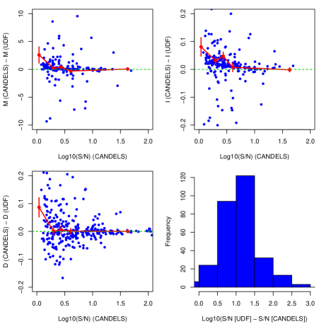
Figure 7: Estimated variation in the $MID$ statistics as a function of the signal-to-noise, $S/N$, between galaxies observed in a sample UDF field ($\approx$78.5 ks exposure) and the same galaxies observed in a $\approx$5.6 ks subexposure (commensurate with typical CANDELS exposure times). The blue dots are individual data and the red curves are estimates of the mean created using five quantiles, i.e., the lowest 20% of CANDELS-exposure $S/N$ values, the next 20%, etc. We find that the $MID$ statistics are insensitive to $S/N$ in the regimes $\gtrsim$ 1.7 ($M$ and $D$) and $\gtrsim$ 3.2 ($I$).

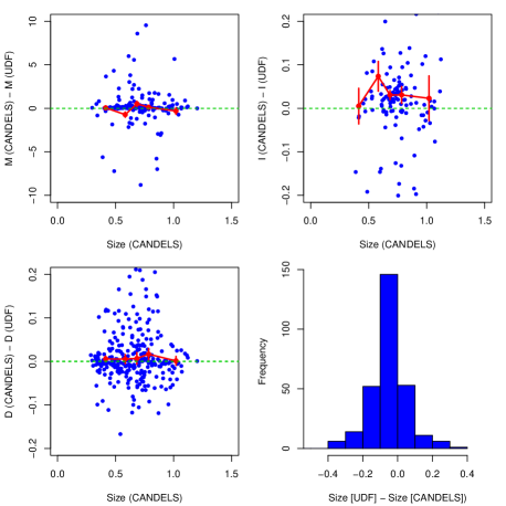
Figure 8: Same as Figure 7, except that estimated galaxy size in arcseconds is plotted along the $x$ axis. We find that the $MID$ statistics are insensitive to galaxy size. The data in the upper right panel are consistent with the null hypothesis of a constant offset from zero. We find the amplitude of this offset is related to the scale of the smoothing kernel applied to the data prior to computing $I$. See §4.4 for more detail.

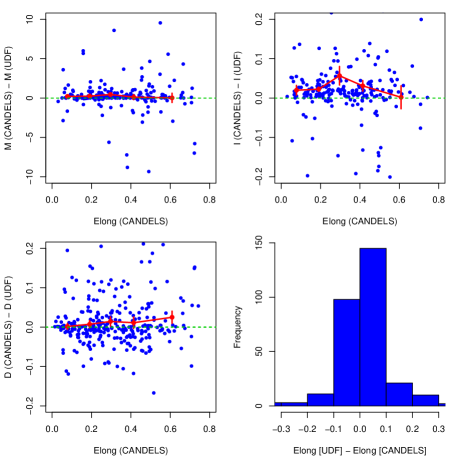
Figure 9: Same as Figure 7, except that estimated galaxy elongation ($1-b/a$) is plotted along the $x$ axis. We find that the $MID$ statistics are insensitive to elongation, with the exception of a systematic increase in $D$ in the regime $\gtrsim$ 0.48. As in Figure 8, we observe that the data in the upper right panel are consistent with the null hypothesis of a constant offset from zero and that the amplitude of this offset is related to the smoothing kernel applied to the data prior to computing $I$. See §4.4 for more detail.

4.5 Effect of galaxy redshift

Having established the regimes in which the $MID$ statistics are (in)sensitive to galaxy $S/N$, size, and elongation, we verify that the ensemble average of the $MID$ statistics increases with redshift, as would expected for statistics that are sensitive to merging activity. In Figure 10, we show the means of the $M$, $I$, and $D$ statistics, as well as their standard errors, as a function of photometric redshift in bins of size $\Delta z=0.2$. To construct this figure, we apply the GOODS-S photometric catalog of Dahlen et al. (2010), which provides $z$ as well as the values $z_{lo}$ and $z_{hi}$ that bound the central 95% of each galaxy’s redshift probability density function (pdf). Lacking further information, we assume the pdf for galaxy $i$ to be a normal pdf with mean $\mu_{i}=(z_{i,hi}+z_{i,lo})/2$ and standard deviation $\sigma_{i}=(z_{i,hi}-z_{i,lo})/3.92$. Then, e.g., the estimated mean of $M$ in redshift bin $j$ is given by

$$\bar{M}(z_{j})=\frac{\sum_{i=1}^{n}w_{ij}M_{i}}{\sum_{i=1}^{n}w_{ij}}\,,$$

where

$$w_{ij}=\Phi\left(\frac{(z_{j}+0.1)-\mu_{i}}{\sigma_{i}}\right)-\Phi\left(\frac{(z_{j}-0.1)-\mu_{i}}{\sigma_{i}}\right)\,.$$

$\Phi(\cdot)$ is the cumulative distribution function for the standard normal distribution. We account for demonstrated biases by excluding the six galaxies for which $S/N<1.7$ in the upper left panel ($M$); the twelve galaxies for which $S/N<3.2$ in the upper right panel ($I$); and the 297 galaxies for which $S/N<1.7$ or $e>0.48$ in the lower left panel ($D$).

Figure 10 shows clear trends between redshift and each of the $MID$ statistics, but we should be careful when quantifying and interpreting these trends because of our assumption of normal pdfs. Thus here we simply assess whether the data are consistent with the null hypothesis of no redshift trend (i.e., zero slope) via weighted linear regression. The $p$ values of the slopes are 8.4 $\times$ 10^-8 ($M$), 1.1 $\times$ 10^-5 ($I$), and 1.2 $\times$ 10^-6 ($D$); we conclude that there are, as we would expect, strong positive correlations between redshift and the $MID$ statistics.

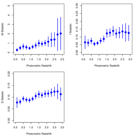
Figure 10: Means and standard errors of the means for the $M$, $I$, and $D$ statistics as a function of photometric redshift in bins of size $\Delta z=0.2$, where the redshifts are provided by the GOODS-S catalog of Dahlen et al. (2010). Via weighted linear regression, we find that the $p$ values of the slopes are 6 $\times$ 10^-8 ($M$), 2 $\times$ 10^-5 ($I$), and 10^-5 ($D$), i.e., we observe strong positive correlations between redshift and the $MID$ statistics. For more details, see §4.5.

5 Examining the annotator’s role

In this section, we explore some of the effects that human annotators have on galaxy morphology analysis. First, we ask whether annotators can accurately label mergers across the regimes of galaxy $S/N$ and size spanned by a single exposure, such as the $H$-band ERS data we analyze above. Then we look towards the future and discuss two important issues: Is it always better to have more annotators looking at each galaxy image? and Ultimately, are annotators even necessary within the context of what we want to achieve, namely, selecting a model of hierarchical structure formation and constraining its parameters?

5.1 Can annotators accurately detect merging activity within a single dataset?

In §4.1, we establish that the $MID$ statistics are useful for detecting non-regular galaxies and merging galaxies that were labeled as such by human annotators. However, we have yet to establish whether labeling is consistent as a function of, e.g., galaxy $S/N$ and size. We construct two equally sized subsets ($n$ = 563) of the 1639 galaxies in our data sample, one where size and $S/N$ are both (relatively) low, and another where size and $S/N$ are both (relatively) high:

$$\hat{r}\leq 0.6^{\prime\prime}~{}~{}{\rm and}~{}~{}\hat{\left(\frac{S}{N}\right)}\leq 15~{}~{} ~{}~{}{\rm``low"}$$

$$\hat{r}>0.6^{\prime\prime}~{}~{}{\rm and}~{}~{}\hat{\left(\frac{S}{N}\right)}>15~{}~{} ~{}~{}{\rm``high"}$$

Both the “low” and “high” datasets contain 563 galaxies. See Figure 11. In Figure 12 we display the distributions of the $M$ statistics for both datasets, for merger vote fractions $f<0.5$, $f=0.5$, and $f>0.5$. We immediately observe a lack of identified mergers ($f>0.5$) with small $M$ values in the “low” dataset. (We note that a similar issue arises in the analysis of regular galaxies, as well as when we use the $I$ statistic in place of $M$.) It is clear from Figure 12 that numerous small-$S/N$/size mergers are being mislabeled, a systematic error that throws into doubt the idea that one can accurately estimate merger fractions at high redshifts via visual labeling. (Note that we base this conclusion on the analysis of a $\approx$50 ks image; typical CANDELS exposures will be one-tenth as long, exacerbating this error.) This result helps motivate the alternative analysis paradigm that we discuss in §5.3.

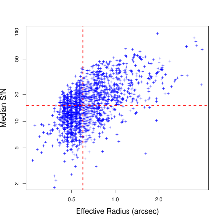
Figure 11: Distribution of effective radius ($\hat{r}$ in text) versus median pixelwise $S/N$ ($\hat{\left(\frac{S}{N}\right)}$ in text) for our 1639-galaxy sample. Dashed lines indicate the values $\hat{r}$ = 0.6$\prime\prime$ and $\hat{\left(\frac{S}{N}\right)}$ = 15. The 563 galaxies each within the lower-left and upper-right regions (as defined relative to where the dashed lines cross) comprise the “low” and “high” datasets respectively.

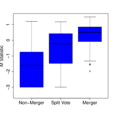
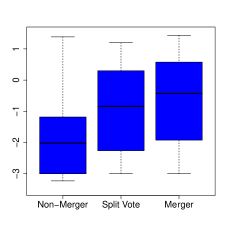
Figure 12: Boxplots showing the distribution of $M$ statistic for identified non-mergers ($f<0.5$), galaxies for which the vote was split ($f=0.5$), and mergers ($f>0.5$). The left and right panels show distributions for the “low” and “high” datasets respectively. The distributions are similar, except for the lack of identified mergers with small $M$ values in the “low” dataset: $M$ clearly correlates with the ability of annotators to identify small-size-and-low-$S/N$ mergers. The behavior of the $I$ statistic between datasets is similar and is not shown.

5.2 The relationship between the number of annotators and classification efficiency

An astronomer’s time is a valuble commodity. Given a set of $N$ astronomers with nominally similar annotation ability, is it best to have all of them train a machine learning algorithm by visually inspecting hundreds if not thousands of galaxy images? Or can using a subset of size $n\ll N$ yield similar detection efficiency?

To attempt to answer these questions, we utilize an analysis carried out by the CANDELS collaboration (Kartaltepe et al. 2012, in preparation) in which 200 objects observed in the $J$- and $H$-bands by the HST WFC3 in the DEEP-JH region of the GOODS-S field were each annotated by 42 voters. The details of voting are similar to those described above in §4, except that in this analysis each annotator’s vote is recorded, so there is no ambiguity about the fraction of annotators identifying particular galaxies as either mergers or non-regulars.

After removing 15 objects from the sample that were subsequently identified as stars (J. Lotz, private communication), we analyze the $H$-band images of the remaining 185 galaxies in a manner similar to that described in §4. The principal difference between analyses is that for computational efficiency, we use only the $MID$ statistics; it is not imperative to use all available statistics because our aim in this analysis is to observe how the estimated risk varies as a function of the number of annotators, $n$, without regard to its actual value.

We assume that a new expert voter will randomly identify a given galaxy $i$ as a non-regular/merger with probability $p_{i}$, where $p_{i}$ is the recorded vote fraction for the set of 42 annotators. Thus to simulate the number of votes for non-regularity/merging for each galaxy, given $n$ annotators, we sample from a binomial distribution with parameters $n$ and $p_{i}$. The result is an integer number of votes $Z_{i}\in[0,n]$, with the simulated vote fraction being $F_{i}=Z_{i}/n$. Given $F$ and the $MID$ statistics for all 185 galaxies, we run random forest and output the estimated risk. We repeat the process of simulation and risk estimation 100 times for each value of $n$ so as to build up an empirical distribution of estimated risk values. Note that as we increase $n$, we only randomly sample new votes. For instance, to go from $n$ = 5 to $n$ = 7, we add two new simulated votes to the five we already have. We feel that this is more realistic than randomly sampling a completely new set of votes, as an increased $n$ in practice generally will be implemented by adding to a core group of annotators rather than replacing that core group in its entirety.

In Figure 13 we display the median of our risk distributions for the non-regular (blue points and lines) and merger (green points and lines) detection cases. The thin and thick lines drawn through each point indicate the range for the central 95 and 68 values in each distribution, respectively. (Note that the values of the risk are generally much higher here than in Tables LABEL:tab:HRNR and LABEL:tab:HNMM because the training sets here are one-ninth the size of those in the analysis of §4.) We observe that for both cases, the estimated risk decreases somewhat sharply when $n\lesssim$ 10; above $n\approx$ 10, the risk for the non-regular case still decreases, albeit more slowly, while the risk for the merger case remains constant. Imprecise estimation of the true vote fractions for small $n$ and vote fraction discretization lead to the increase in risk as $n\rightarrow$ 0, as it becomes less and less likely that, e.g., a “true” merger will be identified as a merger by both annotators and the machine classifier.

For the merger case, it is clear from Figure 13 that little improvement in risk estimation occurs when adding annotators beyond $n\approx 10$. For the non-regular case, there is a slight improvement on average, but there is no guarantee that one would see that improvement in any single analysis. In Figure 14 we show the histogram of the change in risk, $\Delta R$, that occurs as we go from $n=$ 11 to $n=$ 43 annotators; each value is derived from one of our 100 simulations. In 19 of 100 cases, there is an increase in estimated risk; adding 32 annotators made our results worse. This lack of significant improvement in estimated risk, coupled with the time resources that would be expended by the additional annotators, argues strongly that an annotator pool of size $n\approx$ 10 is sufficient for detecting non-regulars.

We conclude that no more than $\approx$10 annotators are needed to effectively train a galaxy morphology classifier using a given set of galaxy images when the goal is to detect non-regular galaxies or mergers. If more annotators are available, they should examine additional sets of galaxy images to increase the overall training set size, and thereby reduce the misclassification risk.

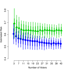
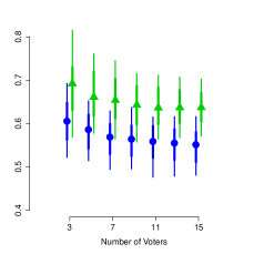
Figure 13: Median estimated risk in the detection of non-regulars (the lower sequence of points in each panel, denoted with blue circles) and mergers (the upper sequence of points in each panel, denoted with green triangles) in the analysis of 185 galaxies described in §5.2, as a function of number of annotators. The right panel shows the same data as the left, for the reduced range $n$ = 3-15. The thin and thick lines drawn through each point represents the central 95% and 68% of the empirical distribution of risk values, respectively. The lines are slightly offset from each other for clarity. See §5.2 for further discussion.

Figure 14: Histogram of the changes in estimated risk that occur when we increase the number of annotators from 11 to 43 in each of the 100 simulations we run in our analysis of 185 galaxies (§5.2). Positive values of $\Delta R$ indicate a reduction in estimated risk. In 19 of 100 simulations, the estimated risk increases: adding annotators led to worse results.

5.3 Towards the future: eliminating visual annotation

As hinted at throughout this work, there are many issues with annotating galaxies and using the resulting morphologies to make quantitative statements about structure formation. Some of the more noteworthy issues are the following:

• Ambiguity. Expert annotators often do not agree on whether a given galaxy is, e.g., undergoing a merger (as opposed to, e.g., undergoing star formation due to in situ disk instabilites). This inability to agree, which led to the large spread of merger fraction estimates compiled by Lotz et al. (2011), is a not-easily quantified source of systematic error: e.g., how does one incorporate the experience and innate biases of each annotator into a statistical analysis? Given the subject of this paper, ambiguity is perhaps an obvious issue to point out, but its deleterious effects on structure formation analysis cannot be overstated.

• Loss of Statistical Information. Above and beyond the issue of ambiguity is the fact that in the classification exercise, we are attempting to take a continuous distribution (e.g., all possible galaxy morphologies) and discretize it (reduce it to, e.g., two bins: mergers and non-mergers). Discretization can only have an adverse effect on statistical inferences, making them certainly less precise and perhaps less accurate.

• Waste of Resources. Annotation is, by definition, a time-consuming exercise that diverts astronomers from other activities.

Our vision of (near) future analyses of galaxy morphology and hierarchical structure formation rests on the belief that simulation engines will be developed that can replicate the wide variety of observed morphologies at a resolution at least on par with current observations. If this occurs, then we can fit structure formation models in the following manner:

1. Populate space of image statistics by analyzing a set of observed galaxies.

2. Pick a set of model parameters describing structure formation.

3. Run a simulator and project the simulated galaxies down onto a (set of) two-dimensional plane(s).

4. Populate a space of image statistics by analyzing the set of simulated galaxy images.

5. Directly compare the estimated distributions of the simulated and observed statistics.

6. Return to step (ii), changing the model parameter values, and iterate until convergence is achieved.

The comparison step, step (v), involves estimating the density functions from which the simulated and observed statistics were sampled, and then determining a “distance” between those functions. There exist numerous, mature methodologies for performing density estimation and estimating distances between density functions. (A summary of possible distance measures is provided in, e.g., Cha 2007.) The key to a computationally efficient comparison is to avoid the “curse of dimensionality”: density estimation is difficult in more than even a few dimensions. Thus even if annotators are no longer needed, there will always be a need to define new statistics that can better disambiguate the morphologies of galaxies.

6 Summary

This work is motivated by the problem of detecting irregular and peculiar galaxies in an automatic fashion in low-resolution and low-S/N images. This information, combined with estimates of galaxy redshift, can help us determine how the merger fraction evolves with time and thus place constraints on theories of hierarchical structure formation. One body of work on irregular/peculiar galaxy detection focuses on the tactic of reducing galaxy images to a set of summary statistics that sufficiently captures morphological details and allows computationally efficient analysis of large samples of galaxies. In particular, the concentration, asymmetry, and clumpiness ($CAS$) statistics of C03 and references therein and the Gini and $M_{20}$ statistics of L04 and references therein have become standard statistics to use in morphological analyses. However, the utility of these statistics to detect the irregularity or peculiarity of high-redshift galaxies is open to question, with simulations by L04 in particular suggesting that the $GM_{20}$ statistics would lose the ability to detect peculiar galaxies in the low-resolution/low-S/N regime.

In an attempt to increase detection efficiency, we have developed three new image statistics$-$the multi-mode ($M$), intensity ($I$), and deviation ($D$) statistics$-$and we test them (along with $CAS$ and $GM_{20}$) on $J$- and $H$-band HST WFC3 images of 1,639 galaxies in the GOODS-South field. In particular, we test these statistics’ abilities to identify both irregular and peculiar galaxies (which we collectively dub “non-regular”) and peculiar galaxies alone (or “mergers”). We use a machine learning-based classifier, random forest, to predict the classes of each of 1,639 galaxies, and we determine its performance by comparing these predictions to visual annotations made by members of the CANDELS collaboration. We strongly advocate the use of random forest or other, similar algorithms such as support vector machines in galaxy morphology studies, as they allow computationally efficient analyses of high-dimensional image-statistic spaces, and thus stand in contrast to the commonly used inefficient technique of projecting these spaces to two-dimensional planes within which classes are identified.

As shown in Figures 4 and 6 and discussed in §§4.1-4.2, we find that our $MID$ statistics, along with the asymmetry statistic $A$, are the most important ones for disambiguating sets of galaxies in our sample; in general, using these four statistics alone yields detection efficiencies on par with using the full set $CAS$-$GM_{20}$-$MID$. In §4.3, we demonstrate that classifier performance is insensitive to the details of the algorithm for constructing segmentation maps, and in §4.4, we find that the $MID$ statistics are largely insensitive to changes in galaxy signal-to-noise, size, and elongation.

We explore the role of human annotators in §5. In §5.1, we construct two subsamples of our dataset, with small-$S/N$/size and large-$S/N$/size galaxies, respectively, to ascertain whether the ability of annotators to label mergers or non-regulars degrades with $S/N$ and size. The difference in appearance of the right-most boxplots in both panels of Figure 12 strongly suggests an inability on the part of annotators to properly label mergers with relatively small values of $M$ in low-$S/N$/size data. (Similar results hold for regulars vs. non-regulars, and if we use $I$ in place of $M$.) Beyond any numbers, this result raises doubt about whether merger rates at high redshift can ever be accurately estimated using annotators.

We next assess how the number of annotators affects classification performance, using a set of 185 $H$-band-observed HST WFC3 images that were each annotated by 42 members of the CANDELS collaboration. We repeatedly sampled subsets of these annotators and used their votes to generate new sets of class predictions, and then we recorded how the estimated risk of making an incorrect prediction varied as a function of the number of annotators (see Figure 13). As discussed in §5.2, we find that there is no evidence that increasing the number of annotators above $n\approx$ 10 yields any improvements in classifier performance for a given set of galaxy images; if more are available, they should be charged with increasing the training set size by annotating additional galaxy images, thereby reducing the risk of misclassification.

As we discuss in §5.3, however, any argument over the optimal number of annotators to deploy within a project may became moot in the future if simulation engines are developed that can effectively recreate the observed populations of galaxies. In our vision of the future, an analyst would populate two spaces$-$one with observed statistics, and one with statistics computed from simulated galaxies$-$and estimate and directly compare the density functions from which the statistics were sampled. In other words, we would quantitatively determine how well the points in the two spaces “line up.” This process would be repeated until an optimal match is found, i.e., until the best-fit model of hierarchical structure formation is found. This methodology effectively sidesteps the issue of, e.g., estimating the merger fraction as a function of redshift, but one could still determine that by, e.g., adopting a definition of “merger” and examining the evolutionary histories of galaxies in the best-fit simulation to see which underwent the process. While annotation is eliminated in this vision, the need for new and improved image statistics is not, since to avoid the “curse of dimensionality” we would always strive to perform density estimation in relatively low-dimensional spaces of image statistics.

Appendix A Implementing random forest using R

R, an open source application for statistical computing available at http://www.r-project.org, is widely used in the statistics community. One of the primary benefits to using R is that one does not have to write code to implement commonly used statistics and machine learning algorithms, which generally exist in one or more packages contributed to the Comprehensive R Archive Network (CRAN). One such package is randomForest, which we utilize here.

After R is downloaded and the GUI is opened, the first step is to install the randomForest package. This may be done by, e.g., tying the following at the prompt within the GUI window and following any subsequent directions:

> install.packages("randomForest")

Before running random forest, however, it is good practice to create a source file, which is a list of commands that can be read into R via the source command (or via the GUI’s pull-down menus). In the following, we assume that the image statistics and the vote fractions are in ASCII text files with single-row headers and one additional row for each galaxy, e.g.,

M         I        D
0.4747    0.3123   0.5666
0.0133    0.0405   0.0259
...

We dub these files statistics.txt and votes.txt.

The following are the contents of a minimalist file that when sourced will run random forest over 1000 splits while assuming that half the galaxies are to be assigned to the training set.

# Input the random forest library functions
library(randomForest)

# Input the dependent (votes) and
#   independent (statistics) data
# Assume the first row of votes is:
#   "nonreg merger"
# Assume the first row of statistics is:
#   "M I D"
#
votes = read.table("votes.txt",header=T)$merger
stats = read.table("statistics.txt",header=T)

# Standardize the statistics column-by-column:
#   X_i -> (X_i-mean(X))/sd(X)
#
stats = scale(stats)

# Specify the (sub)set of statistics to input to
#   random forest.
set = c("M","I","D")

# Here we assume no ties that have to be broken.
class = votes>0.5

ntrain = round(0.50*length(data[,1]))
B = 1000

# Initialize vectors of length B
sens = spec = risk = toterr = ppv = npv = rep(-9,B)

for ( ii in 1:B ) {
  # assign galaxies to training/test sets
  train     = sample(1:length(stats[,1]),size=ntrain)
  test      = (1:length(stats[,1]))[-train]
  # run random forest regression -- Section 3.1
  fit       = randomForest(x=stats[train,set],
                           y=votes[train],
                           maxnodes=8)
  predTrain = predict(fit,stats[train,set])
  predTest  = predict(fit,stats[test,set])
  # determine the class threshold -- Section 3.2
  cut = seq(0,1,0.001)
  c0 = NULL
  c1 = NULL
  for ( ii in 1:length(cut) ) {
    c0 = append(c0,
         mean(predTrain[class[train]==0]>cut[ii]))
    c1 = append(c1,
         mean(predTrain[class[train]==1]<cut[ii]))
  }
  smooth = ksmooth(cut,colMeans(rbind(c0,c1)),
                   bandwidth=0.05)
  mc = smooth$x[which.min(smooth$y)]
  # record the important quantities -- Section 3.3
  sens[ii]   = 1-mean(predTest[class[test]==1]<mc)
  spec[ii]   = 1-mean(predTest[class[test]==0]>=mc)
  risk[ii]   = mean(predTest[class[test]==1]<mc)+
               mean(predTest[class[test]==0]>mc)
  toterr[ii] = mean((predTest>mc)!=class[test])
  ppv[ii]    = 1-mean(class[test][predTest>mc]==0)
  npv[ii]    = 1-mean(class[test][predTest<=mc]==1)
}

# Output the mean estimated risk over all B splits
#   (other values can be output in a similar manner).
cat("Estimated Risk = ",mean(risk),"\n")

q()

Once this file is saved to disk (we dub this file rf_source.R), it may be sourced via the “Source File…” option in the R GUI’s pull-down menu, or by typing

> source("<path>/rf_source.R")

References

- Abraham, van den Bergh, & Nair (2003) Abraham, R. G., van den Bergh, S., Nair, P. 2003, ApJ, 588, 218
- Bershady, Jangren, & Conselice (2000) Bershady, M. A., Jangren, A., Conselice, C. J. 2000, AJ, 119, 2645
- Bertone & Conselice (2009) Bertone, S., Conselice, C. J. 2009, MNRAS, 396, 2345
- Bertin & Arnouts (1996) Bertin, E., Arnouts, S. 1996, A&AS, 117, 393
- Bluck et al. (2012) Bluck, A. F. L., et al. 2012, ApJ, 747, 34
- Breiman (2001) Breiman, L. 2001, Machine Learning, 45, 5
- Bridge, Carlberg, & Sullivan (2010) Bridge, C. R., Carlberg, R. G., Sullivan, M. 2010, ApJ, 709, 1067
- Cha (2007) Cha, S.-H. 2007, IntJMathModMethAppSci, 1, 300
- Chen, Lowenthal, & Yun (2010) Chen, Y., Lowenthal, J. D., Yun, M. S. 2010, ApJ, 712, 1385
- Conselice, Bershady, & Jangren (2000) Conselice, C. J., Bershady, M. A., Jangren, A. 2000, ApJ, 529, 886
- Conselice (2003) Conselice, C. J. 2003, ApJS, 147, 1 (C03)
- Conselice et al. (2003) Conselice, C. J., Bershady, M. A., Dickinson, M., Papovich, C. 2003, AJ, 126, 1183
- Conselice, Rajgor, & Myers (2008) Conselice, C. J., Rajgor, S., Myers, R. 2003, MNRAS, 386, 909
- Conselice et al. (2011) Conselice, C. J. et al. 2011, MNRAS, 417, 2770
- Dahlen et al. (2010) Dahlen, T. et al. 2010, ApJ, 724, 425
- Darg et al. (2010) Darg, D. W. et al. 2010, MNRAS, 401, 1043
- Grogin et al. (2011) Grogin, N. A. et al. 2011, ApJS, 197, 35
- Hastie, Tibshirani, & Friedman (2009) Hastie, T., Tibshirani, R., Friedman, J. 2009, The Elements of Statistical Learning (2nd Edition), Springer (HFT09)
- Holwerda et al. (2011) Holwerda, B. W. et al. 2011, MNRAS, 416, 2401
- Hopkins et al. (2010) Hopkins, P. F. et al. 2010, ApJ, 724, 915
- Hoyos et al. (2012) Hoyos, C. et al. 2012, MNRAS, 419, 2703
- Jogee et al. (2009) Jogee, S. et al. 2009, ApJ, 697, 1971
- Kartaltepe et al. (2010) Kartaltepe, J. et al. 2010, ApJ, 721, 98
- Koekemoer et al. (2011) Koekemoer, A. M. et al. 2011, ApJS, 197, 36
- Kutdemir et al. (2010) Kutdemir, E., Ziegler, B. L., Peletier, R. F., Da Rocha, C., Böhm, A., Verdugo, M. 2010, A&A, 520, 109
- Law et al. (2007) Law, D. R. et al. 2007, ApJ, 656, 1
- Lintott et al. (2008) Lintott, C. J. et al. 2008, MNRAS, 389, 1
- Lisker (2008) Lisker, T. 2008, ApJS, 179, 319
- Lotz, Primack, & Madau (2004) Lotz, J. M., Primack, J., Madau, P. 2004, AJ, 128, 163 (L04)
- Lotz et al. (2006) Lotz, J. M., Madau, P., Giavalisco, M., Primack, J., Ferguson, H. C. 2006, ApJ, 636, 592
- Lotz et al. (2008) Lotz, J. M. et al. 2008, ApJ, 672, 177
- Lotz et al. (2010a) Lotz, J. M., Jonsson, P., Cox, T. J., Primack, J. R. 2010, MNRAS, 404, 575
- Lotz et al. (2010b) Lotz, J. M., Jonsson, P., Cox, T. J., Primack, J. R. 2010, MNRAS, 404, 590
- Lotz et al. (2011) Lotz, J. M., Jonsson, P., Cox, T. J., Croton, D., Primack, J. R., Somerville, R. S., Stewart, K. 2010, ApJ, 742, 103
- Mendez et al. (2011) Mendez, A. J., Coil, A. L., Lotz, J., Salim, S., Moustakas, J., Simard, L. 2011, ApJ, 736, 110
- Peng et al. (2002) Peng, C. Y., Ho, L. C., Impey, C. D., Rix, H.-W. 2002, AJ, 124, 266
- Windhorst et al. (2011) Windhorst R. A. et al. 2011, ApJS, 193, 27