Searching with and against the stream: Lévy or Brown?

Abstract

We study the efficiency of search processes based on Lévy flights (LFs) with power-law distributed jump lengths in the presence of an external drift. While LFs turn out to be efficient search processes when relative to the starting point the target is upstream, in the downstream scenario regular Brownian motion turns out to be advantageous. This is caused by the occurrence of leapovers of LFs, due to which LFs typically overshoot a point in space. We establish criteria when the combination of the external stream and the initial distance between the starting point and the target favors LFs over regular Brownian search. Contrary to the common belief that LFs with a stable index $\alpha=1$ are optimal, we find that the optimal $\alpha$ may range in the entire interval $(1,2)$ and even include Brownian motion as the overall most efficient search strategy.

How do you find a needle in a haystack? Scientists have studied the dynamics and optimization of search processes for decades, their interest ranging from military tasks such as locating enemy submarines, over search strategies of animals for food, to diffusion control of molecular processes in biological cells olivier ; gandhi . Without prior knowledge about the location of the target, a searcher randomly explores the search space. However, as already argued by Shlesinger and Klafter shlekla , instead of performing a Brownian walk a better search strategy for sparse targets is that of a Lévy flight (LF): the agent moves randomly with a power-law distribution $\lambda(x)\simeq|x|^{-1-\alpha}$ of relocation lengths. Due to their lack of a length scale, LFs combine local exploration with decorrelating, long-range excursions, and are thus more efficient than searchers following a Gaussian form of $\lambda(x)$ viswanathan ; bartumeus .

There exist competing random search models, such as intermittent dynamics switching between local diffusive search and ballistic relocations intermittent , or persistent random walk models persist . However, while the difference in performance is small michael , the central advantage of LF strategies is the robustness: while other models work best when their parameters are optimized for specific environmental conditions (e.g., the target density), LFs remain close to optimal even when these conditions change michael . LFs are thus a preferred strategy when there is insufficient prior knowledge on the search space. Indeed, power-law relocation statistics were observed for a variety of species, including mussels mussels , plant lice aphids , bats bats , marine predators sharks , spider monkeys spider , and even for human motion patterns humans . LFs also emerge naturally in models for molecular gene regulation michael1 . We note that LFs in the biological context are often categorized as saltatory motion james .

What happens when the search process is biased? This may occur naturally, when sharks search in areas with an underwater stream or bats forage on a windy night. Similarly, this may happen in search algorithms when the complex search space has an overall tilt. As we show here based on a new definition of the search efficiency relevant for a single target, the answer to the question for the optimal search strategy crucially depends on the presence of such streams, in particular, whether the stream is towards or away from the target. We also show that complementary criteria for the optimization of the search process lead to different answers for what is the best search strategy. Thus, Brownian search may be more efficient than LF search when the stream is towards the target or, alternatively, when the target happens to be close to the searcher. Conversely, LF search wins out when the target is difficult to locate. Our results shed new light on the long-standing question of optimization in random search processes.

Figure 1: Scheme of the search process. A random walker performs random jumps in the search space until hitting the target. Here, the search is biased by a drift away from the target. Such an uphill drift caused, for instance, by underwater streams or above-ground winds affects the search efficiency.

First arrival time. Consider the scenario sketched in Fig. 1. A random walker searches for the target by performing random jumps. These are biased by an external drift. We refer to the bias as downhill when the target lies in the direction of the stream as seen from the initial position of the random walker and vice versa. Discovery of the target then corresponds to the process of first arrival of the walker at the target position. We recall that for LFs long leapovers with length distribution $p(\ell)\simeq\ell^{-1-\alpha/2}$ across a point may frequently occur, and thus the probability to actually arrive at a point is significantly smaller than the passage of the walker across this point koren ; fpt . As basis for our description we use the fractional Fokker-Planck equation (FFPE) for LFs in the presence of the drift velocity $v$ report ,

$$\frac{\partial f(x,t)}{\partial t}=\frac{\partial^{\alpha}f(x,t)}{\partial\left|x\right|^{\alpha}}-v\frac{\partial f(x,t)}{\partial x}-\wp_{\mathrm{fa}}(t)\delta(x)$$ (1)

defined for $0<\alpha\leq 2$. The distribution $f(x,t)$ is the density function to find the walker at position $x$ at time $t$, for which we assume the initial position $x_{0}$, i.e., $f(x,0)=\delta(x-x_{0})$. The fractional derivative $\partial^{\alpha}/\partial|x|^{\alpha}$ is defined in terms of its Fourier transform, $\int_{-\infty}^{\infty}e^{ikx}\partial^{\alpha}/\partial|x|^{\alpha}f(x,t)dx=-|k|^{\alpha}f(k,t)$, where $f(k,t)=\int_{-\infty}^{\infty}e^{ikx}f(x,t)dx$ is the Fourier transform of $f(x,t)$ REM . Thus, in the limit $\alpha=2$ we recover the standard Fokker-Planck equation of Brownian motion. In Eq. (1), we introduced rescaled, dimensionless variables, such that $v$ is a measure for the amplitude of the drift (see the Supplementary Material for the rescaling of the FFPE supp ). In Eq. (1) we implemented a point sink at $x=0$ representing the target: the random walker is removed when the target is hit. Here, $\wp_{\mathrm{fa}}(t)$ is the density of first arrival. Eq. (1) generalizes the first arrival dynamics in absence of a drift of Ref. fpt . Due to the sink term, the density function $f(x,t)$ is not normalized, that is, the cumulative survival $\mathscr{S}(t)=\int_{-\infty}^{\infty}f(x,t)dx$ is a decreasing function of time. Using the properties of the fractional derivative, integration of Eq. (1) over the position coordinate $x$ delivers the first arrival density, $\wp_{\mathrm{fa}}(t)=-(d/dt)\int_{-\infty}^{\infty}f(x,t)dx=-(d/dt)\mathscr{S}(t)$.

The solution of Eq. (1) can be obtained via Fourier-Laplace transform, and for $\wp_{\mathrm{fa}}$ we find

$$\wp_{\mathrm{fa}}(s)=\int_{-\infty}^{\infty}e^{ikx_{0}}\xi dk\Big{/}\int_{-\infty}^{\infty}\xi dk,\xi=(s+|k|^{\alpha}-ikv)^{-1},$$ (2)

where the Laplace transform is defined as $f(x,s)=\int_{0}^{\infty}e^{-st}f(x,t)dt$. Result (2) instantly shows an important feature: for discontinuous LFs with $0<\alpha\leq 1$, the quantity $\wp_{\mathrm{fa}}(s)$ vanishes, since the integral in the denominator diverges while the integral in the numerator converges. Thus Lévy search for a point-like target will never succeed for $0<\alpha\leq 1$. This property reflects transience of Lévy flights with $\alpha<d$, where $d$ is the embedding spatial dimension sato . In this sense the value $\alpha=1$ obtained for optimal search for sparse targets in drift-free search gandhi ; michael1 is to be seen as limiting point of $\alpha$ from above unity. We obtained analytical results for the first arrival behavior encoded in Eq. (2) in the limit of a small bias, see SM supp . In the following we combine numerical analysis and complementary definitions of the search efficiency to study the optimal random search of Brownian versus LF strategies.

Search efficiency. What is a good measure for the efficiency of a search mechanism? There are two frequently used definitions of search efficiency, counting the number of found targets either per traveled unit distance or per number of steps james . These definitions work well when there is a finite target density. Here we are interested in the more natural problem of search for a single target, a countable number of targets, or a finite target area. In such cases the average search time diverges, and we thus need a modified definition for the search efficiency. We choose the average over inverse search times,

$$\mathcal{E}=\left<\frac{1}{t}\right>=\int_{0}^{\infty}\wp_{\mathrm{fa}}(s)ds,$$ (3)

where $\langle\cdot\rangle=\int_{0}^{\infty}\cdot\wp_{\mathrm{fa}}(t)dt$. Due to the definition of $\mathcal{E}$ as inverse first arrival times, contributions from short and intermediate times dominate the efficiency. To demonstrate the usefulness of definition (3) we determined $\mathcal{E}$ for a Brownian searcher for both downhill and uphill situations with arbitrary $v$ and $x_{0}>0$. We find respectively,

$$\mathcal{E}=\frac{2}{x_{0}^{2}}\left(1+\frac{|v|x_{0}}{2}\right)\left\{\begin{array}[]{ll}1,&v\leq 0\\[5.69046pt] \exp\left(-vx_{0}\right),&v\geq 0\end{array}\right.$$ (4)

Consistently we observe that the search efficiency increases with $v$ when the stream pushes the searcher towards the target, while the efficiency decreases exponentially in the uphill case. The latter can be interpreted as an activation barrier for target detection. In absence of a drift the efficiency is just the inverse mean diffusion time (on average, $x_{0}^{2}\sim 2t$ in dimensionless units).

Combining expressions (S4) and (3) we obtain the search efficiency for an LF in the presence of a weak bias,

$$\mathcal{E}=\frac{\alpha}{x_{0}^{\alpha}}\left[\cos\left(\pi\left[1-\frac{\alpha}{2}\right]\right)\Gamma(\alpha)-2\left(1-\frac{1}{\alpha}\right)\mathrm{Pe}_{\alpha}\right],$$ (5)

for $1<\alpha\leq 2$. Here we introduced the generalized Péclet number $\mathrm{Pe}_{\alpha}=vx_{0}^{\alpha-1}/2$. Note that $\mathrm{Pe}_{\alpha}$ is in fact dimensionless, due to the rescaling of variables, see Eq. (1). This is our first main result. In the Brownian limit $\alpha=2$ the efficiency is $\mathcal{E}\simeq 2x_{0}^{-2}(1-\mathrm{Pe}_{2})$, which corresponds to the small $v$-expansion in Eq. (4). For $\alpha\rightarrow 1$ and with $x_{0}$ fixed the efficiency drops to zero. While $\alpha=1$ is the optimal parameter for LF search of sparse but finite target density, for the case considered here the transition to discontinuous LFs at $\alpha=1$ means that the target can no longer be detected. These observations show that the standard dogmas on the efficiency of random search processes are much more specific than usually believed.

Let us discuss the efficiency of LF search in more detail, starting with the case of vanishing drift strength $v$. As the time to reach the target grows substantially with initial distance $x_{0}$, we compare the search efficiency at fixed value $x_{0}$. In Fig. 2 we show the dependence on the stable index $\alpha$ of the relative efficiency $\mathcal{E}_{\mathrm{rel}}=\mathcal{E}/\mathcal{E}_{\mathrm{opt}}$, where $\mathcal{E}_{\mathrm{opt}}$ is the maximal value of $\mathcal{E}$ for given $x_{0}$ attained at the optimal stable index $\alpha_{\mathrm{opt}}$. We observe that when the starting point of the walker $x_{0}$ is close to the target, the optimal search strategy is Brownian. This is intuitively clear: Brownian motion cannot overshoot the target and therefore leads to quick localization. For more distant targets the oversampling of Brownian walks, i.e., the tendency to multiply return to previously visited points, reduces the Brownian efficiency, and LFs win out. This is shown for the larger $x_{0}$ values in Fig. 2. Interestingly, the behavior of $\mathcal{E}_{\mathrm{rel}}$ is non-monotonic, and becomes sharper for increasing $x_{0}$. In the limit of very large $x_{0}$ the optimal value of the stable index $\alpha$ tends to unity. The non-monotonicity of $\mathcal{E}_{\mathrm{rel}}$ is one of our central results.

Figure 2: Left: Relative efficiency $\mathcal{E}_{\mathrm{rel}}$ for LFs with $v=0$ as function of stable index $\alpha$, Eq. (5). The curves are drawn for the initial positions $x_{0}=1$ (black full line), $x_{0}=10$ (red dashed), $x_{0}=100$ (blue dotted) and $x_{0}=1,000$ (pink dash-dotted). With growing $x_{0}$ the functional shape changes from a monotonic to non-monotonic shape and then becomes sharper, their maximum shifting towards unity. Thus, for $x_{0}=10$ we find $\alpha_{\mathrm{opt}}\approx 1.5$, while for $x_{0}=1000$, $\alpha_{\mathrm{opt}}\approx 1.15$. Right: Optimal stable index $\alpha_{\mathrm{opt}}$ as function of the initial position $x_{0}$, as obtained from Eq. (6). For $x_{0}\lessapprox 2.516$, the optimal search strategy is Brownian (shaded area).

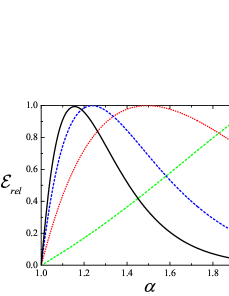
At fixed starting position $x_{0}$ and in absence of a drift the implicit expression to determine the optimal stable index $\alpha_{\mathrm{opt}}$ follows from $\left.d\mathcal{E}/d\alpha\right|_{\alpha_{\mathrm{opt}}}=0$, the result being

$$x_{0}=2\exp\left\{\frac{1}{\alpha_{\mathrm{opt}}}+\frac{1}{2}\psi\left(\frac{\alpha_{\mathrm{opt}}}{2}\right)+\frac{1}{2}\psi\left(\frac{1-\alpha_{\mathrm{opt}}}{2}\right)\right\}.$$ (6)

Here $\psi$ denotes the digamma function. Eq. (6) allows us to plot $\alpha_{\mathrm{opt}}$ as function of the initial position of the LF searcher shown in Fig. 2. Interestingly, if for our dimensionless units the initial position is closer to the target than $x_{0}\approx 2.516$, then the optimal search strategy is Brownian, otherwise it corresponds to LFs with $\alpha_{\mathrm{opt}}$.

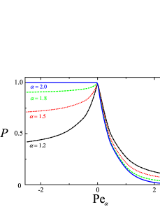
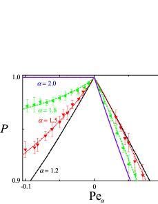
Once an external drift is present, the arrival to the target as function of the initial position $x_{0}$ and the drift strength $v$ becomes non-trivial. In particular, there may exist a finite residual survival probability $\lim_{t\to\infty}\mathscr{S}(t)$. The probability $P=\int_{0}^{\infty}\wp_{\mathrm{fa}}(t)dt=1-\lim_{t\to\infty}\mathscr{S}(t)$ to successfully reach the target quantifies the ability of the process to ever reach the target. For some purposes this measure may be more relevant than the efficiency $\mathcal{E}$. A large value of $P$ for given parameters corresponds to a high success probability to eventually locate the target. $P$ is displayed for a large range of the generalized Péclet number $\mathrm{Pe}_{\alpha}$ in Fig. 3. In addition, Fig. 3 depicts the small-$\mathrm{Pe}_{\alpha}$ case. These results are obtained from numerical solution of Eq. (2) and are thus not restricted to small values of $\mathrm{Pe}_{\alpha}$ SimulDetails . From dimensional analysis it is straightforward to show that the success probability $P$ solely depends on the single parameter $\mathrm{Pe}_{\alpha}$.

In the downhill case, when the searcher is pushed towards the target by the external stream ($\mathrm{Pe}_{\alpha}<0$) the best strategy in terms of $P$ is always that of Brownian search, reaching $P=1$ for all values of $\mathrm{Pe}_{\alpha}$. The LF searcher in this regime always fares worse ($P<1$), the discrepancy increasing for smaller values of the stable index. This is due to the occurrence of leapovers across the target for LFs. In the presence of a strong drift, the success probability $P$ becomes considerably smaller. The opposite tendency is observed for the uphill case when the walker needs to move against the stream towards the target ($\mathrm{Pe}_{\alpha}>0$). Now, LFs with a smaller stable index perform better, due to the possibility to approach the target faster with fewer jumps. We note, however, that the absolute gain of LF versus Brownian search in the uphill case is considerably smaller than the loss in the downhill scenario.

Figure 3: Left: Dependence of the cumulative first arrival probability on the Peclét number $\mathrm{Pe}_{\alpha}$. Lines are from numerical solution of Eq. (2). The blue (full) line corresponds to Brownian search, $\alpha=2$, the green (dashed) represents LF search with $\alpha=1.8$, and the red (dotted) line stands for $\alpha=1.5$. Finally, the black (dashed-dotted) line is for $\alpha=1.2$. Right: Same for small values of $\mathrm{Pe}_{\alpha}$. In addition to the numerical solution of Eq. (2), the symbols and error bars are obtained from Langevin equation simulations of LF trajectories. Coloring and lineshapes correspond to Fig. 3.

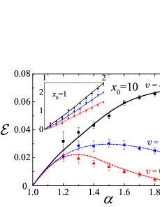
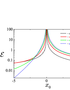
The search efficiency $\mathcal{E}$ is affected by the external stream even more dramatically than the success probability $P$, as shown in Fig. 4. Here, the initial position is fixed at $x_{0}=10$ in the main Figure, and $x_{0}=1$ in the inset. Black (full) lines correspond to the downhill case with $v=-0.5$, and the red (dashed) curves to the uphill case with $v=0.5$. The neutral case $v=0$ is shown by the blue (dotted) line. For $\alpha\rightarrow 1$ the curves converge, in the case $x_{0}=10$ they almost coincide below $\alpha\approx 1.15$. In the case without bias and $x_{0}=1$, consistent with our observations in the drift-free case above, the optimal strategy remains Brownian (see Fig. 2). In contrast, for the larger initial separation $x_{0}=10$ the downhill case the optimal search strategy is also Brownian, while without bias we found $\alpha_{\mathrm{opt}}\approx 1.5$. In the uphill case the optimal stable index is shifted to $\alpha_{\mathrm{opt}}\approx 1.3$. The delicate behavior of $\alpha_{\mathrm{opt}}$ is our other important finding.

Figure 4: Left: Efficiency as a function of stable index $\alpha$ for initial positions $x_{0}=10$ and $x=1$ (Inset). We show the downhill case ($v=-0.5$, full black curve), neutral case ($v=0$, blue dotted curve), and uphill case ($v=0.5$, red dashed curve). Right: Efficiency versus initial position $x_{0}$ for $v=-1.0$, i.e., negative $x_{0}$ correspond to uphill motion.

Discussion. So what is now the best search strategy? As we showed here this depends crucially on what is more important: to reach the target quickly or to locate it with the highest likelihood. Moreover, the answer to this question also depends on the situation, whether there is a single or few targets, or whether we face a constant density of targets. It will be interesting to study such questions in Lévy search models for finite target density.

Specifically, we investigated the performance of LF search models along or against an external stream. Defining the efficiency as the average inverse arrival time $\left<1/t\right>$ to the target, we obtained a versatile measure to quantify search processes when the search space does not have a constant target density. This efficiency $\left<1/t\right>$ reproduces the features of Brownian search and works well for both unbiased and biased search processes, unlike the similar construct $1/\left<t\right>$. In terms of this efficiency we investigate the optimal search strategy, comparing Lévy and Brownian search processes. Without an external bias, it turns out that the optimal strategy depends on the initial separation between the searcher and the target: for small separations Brownian motion is the most efficient way of finding the target. On increasing this separation LFs become more and more efficient in comparison to Brownian search, and the stable index $\alpha$ decreases towards unity in the limit of very large initial searcher-target separation. In particular, we find that despite the common claim that LFs with $\alpha=1$ are most efficient, depending on the parameters of the search space the optimal stable index may range in the whole interval between unity and two.

When the searcher moves with or against an external stream the analysis in terms of the success probability $P$ shows that when the initial position of the searcher with respect to the target is along the stream, the optimal search strategy is always Brownian, due to the combined effect of biased motion and absence of the leapovers in the case of LFs. The average search time is then simply given in terms of the ratio of initial searcher-target separation and the drift velocity $v$. When the searcher needs to reach the target against the stream, LFs provide the better search strategy. This trend is confirmed by the results for the success probability $P$. Remarkably, the gain from using the Brownian strategy instead of LFs in the downhill scenario is significantly larger than the loss from using Brownian motion instead of LFs in the uphill case. Depending on the details of the search space, without prior knowledge on the strength and direction of external streams, the choice of a Brownian strategy might therefore be overall advantageous, in contrast to the general dogma in favor of Lévy search. These observations may be of particular importance to swimming or airborne searchers, as streams occur most naturally there. They may also be relevant for computational search algorithms in biased landscapes.

VVP acknowledges discussions with A. Cherstvy and financial support from Deutsche Forschungsgemeinschaft. RM acknowledges financial support from the Academy of Finland (FiDiPro scheme).

References

- (1) O. Bénichou, C. Loverdo, M. Moreau and R. Voituriez, Rev. Mod. Phys., 83, 81 (2011); P. C. Bresloff, J. M. Newby, Rev. Mod. Phys. 85, 135 (2013); M. F. Shlesinger, J. Phys. A 42, 434001 (2009).
- (2) G. M. Viswanathan, M. G. E. da Luz, E. P. Raposo, and H. E. Stanley, The Physics of Foraging. An Introduction to Random Searches and Biological Encounters (Cambridge University Press, New York, 2011).
- (3) M. F. Shlesinger and J. Klafter in On Growth and Form, edited by H. E. Stanley and N. Ostrowsky (Martinus Nijhoff, Dordrecht, 1986).
- (4) G. M. Viswanathan, S. V. Buldyrev, S. Havlin, M. G. E. da Luz, E. P. Raposo and H. E. Stanley, Nature 401, 911 (1999).
- (5) F. Bartumeus, J. Catalan, U. L. Fulco, M. L. Lyra, and G. M. Viswanathan, Phys. Rev. Lett. 88, 097901 (2002).
- (6) O. Bénichou, M. Coppey, M. Moreau, P. H. Suet, and R. Voiturierz, Phys. Rev. Lett. 94, 198101 (2005); C. Loverdo, O. Bénichou, M. Moreau, and R. Voiturierz, Nature Phys. 4, 134 (2008); compare also S. Benhamou, Ecology 88, 1962 (2007); A. Reynolds, Physica A 388, 561 (2009).
- (7) P. Bovet and S. Benhamou, J. Theoret. Biol. 131, 419 (1988).
- (8) M. A. Lomholt, T. Koren, R. Metzler, and J. Klafter, Proc. Natl. Acad. Sci. USA 105, 11055 (2008).
- (9) M. de Jager, F. J. Weissing, P. M. J. Herman, B. A. Nolet, and J. van de Koppel, Science 332, 1551 (2011).
- (10) A. Mashanova, T. H. Oliver, V. A. A. Jansen, J. R. Soc. Interface 7, 199 (2010).
- (11) M. G. Lundy, A. Harrison, D. J. Buckley, E. S. Boston, D. D. Scott, E. C. Teeling, W. I. Montgomery, and J. D. R. Houghton, J. R. Soc. Interface 10, 20120489 (2012).
- (12) D. W. Sims et al., Nature, 451, 1098 (2008); N. E. Humphries et al., ibid., 465, 1066 (2010).
- (13) G. Ramos-Fernández, J. L. Mateos, O. Miramontes, G. Cocho, H. Larralde, B. Ayala-Orozco, Behav. Ecol. Sociobiol.55, 223 (2004)
- (14) M. C. González, C. A. Hidalgo, and A.-L. Barabási, Nature 453, 779 (2008); D. Brockmann, Phys. World (2), 31 (2010).
- (15) M.A. Lomholt, T. Ambjörnsson, and R. Metzler, Phys. Rev. Lett. 85, 260603 (2005).
- (16) A. James, J. W. Pitchford, M.J. Plank, Bull. Math. Biol. 72, 896 (2010).
- (17) A. V. Chechkin, R. Metzler, V. Yu. Gonchar, J. Klafter and L. V. Tanatarov, J. Phys. A 36, L537 (2003).
- (18) T. Koren, M. A. Lomholt, A. V. Chechkin, J. Klafter, and R. Metzler, Phys. Rev. Lett., 99, 160602 (2007); T. Koren, A. V. Chechkin, and J. Klafter, Physica A 379, 10 (2007).
- (19) R. Metzler and J. Klafter, Phys. Rep. 339, 1 (2000); J. Phys. A 37, R161 (2004).
- (20) For an explicit definition of the fractional derivative, see the Supplementary Material supp .
- (21) Supplementary Material.
- (22) K.-I. Sato, Lévy processes and infinitely divisible distributions (Cambridge University Press, Cambridge, UK 1999).
- (23) Increase of values increases the LE simulation time. We confirmed FFPE results with LE simulation for (Fig. 3) with very good agreement. Each simulation point was obtained as a ratio of trapped particles to the overall number of 10,000 runs. We estimated error bars by computation of the deviations for each of consecutive 1,000 runs.