Bunching coefficients in Echo-Enabled Harmonic Generation

Abstract

Coulombian diffusion determines a dilution of bunching coefficients in Free Electron Laser seeded devices. From the mathematical point of view the effect can be modeled through a heat type equation, which can be merged with the ordinary Liouville equation, ruling the evolution of the longitudinal phase space beam distribution. We will show that the use of analytical tools like the Generalized Bessel Functions and algebraic techniques for the solution of evolution problems may provide a useful method of analysis and shine further light on the physical aspects of the underlying mechanisms.

I Introduction

In this paper we will pursue some technical details concerning the computation and the physical understanding of the recent analysis by Stupakov Stupakov1 on the effect of Coulomb diffusion on bunching coefficients in Echo Enabled Harmonic Generation (EEHG) Free Electron Laser (FEL) seeded devices Stupakov2 . The considerations developed in this paper should be understood as a complement to refs. Stupakov1 ; Stupakov2 , with the aim of providing a more general computational framework, benefitting from the formalism of beam transport employing algebraic means Dattoli1 . In this treatment the transport through magnetic elements is treated in terms of exponential operator acting on an initial phase space distribution and usually do not contain “transport” elements provided by a heat type diffusion. Here we will show that diffusion mechanisms can be included in such a framework in a fairly straightforward way Dragt , preserving the spirit of exponential operator concatenation.

The effect of the Coulomb diffusion on the e-beam longitudinal phase space distribution is ruled, according to Stupakov1 , by the equation

$$\partial_{s}f\left(p,\zeta,s\right)=D\partial_{p}^{2}f(p,\zeta,s),$$ (1)

$$f(p,\zeta,0)=f_{0}(p,\zeta)$$

Where $s$ is the coordinate of propagation, $\zeta$ is the longitudinal coordinate in the beam, $p$ is associated to the beam energy, $D$ is the Coulomb diffusion coefficient and $f_{0}\left(p,\zeta\right)$ is the “initial” distribution. We will discuss the physical meaning of the previous quantities and we will provide their explicit expression in the following, for the moment we note that, having assumed that $D$ is independent of $p$ , we can solve (1) via the following Gauss-Weierstrass (G-W) transform Babusci

$$f\left(p,\zeta,s\right)=\frac{1}{2\sqrt{\pi Ds}}\int_{-\infty}^{\infty}e^{-\frac{\left(p-\eta\right)^{2}}{4Ds}}f_{0}(\eta,\zeta)d\eta$$ (2)

The bunching coefficients can be defined as those of the Fourier components of the expansion Dattoli2

$$f\left(p,\zeta,s\right)=\sum_{n=-\infty}^{+\infty}b_{n}\left(p,s\right)e^{in\zeta}$$ (3)

and are, therefore, specified by

$$b_{m}(p,s)=\frac{1}{2\pi}\int_{0}^{2\pi}d\zeta f\left(p,\zeta,s\right)e^{-im\zeta},$$ (4)

The dilution of the bunching coefficients induced by the Coulomb diffusion can therefore be mathematically expressed as

$$b_{m}(p,s)=\frac{1}{2\sqrt{\pi Ds}}\int_{-\infty}^{\infty}e^{-\frac{\left(p-\eta\right)^{2}}{4Ds}}b_{m}(\eta)d\eta$$ (5)

Following ref. Stupakov1 , we assume the initial distribution

$$f_{0}(p,\zeta)=\frac{1}{\sqrt{2\pi}}e^{-\frac{\left[p-A_{1}\sin\left(\zeta-B_{1}p\right)\right]^{2}}{2}}$$ (6)

whose physical meaning will be discussed in the forthcoming section. The solution of eq. (1) can be therefore easily computed, even though cannot be obtained in analytical form. In Fig. 1 we have reported the effect of the dispersion on the initial distribution (Fig. 1a), after a drift $s=0.3$ with $D=0.7$ (Fig. 1b).

      

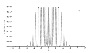
Figure 1: Evolution of the distribution function $f(p,\zeta,s)$ undergoing the coulombian diffusion. a) $f(p,0,0),\>A_{1}=3,\>B_{1}=8.47$ b) $f(p,0,0.3),\>A_{1}=3,\>B_{1}=8.47,\>D=0.7$.

It is evident that the Coulomb term smears out the oscillations, associated with the bunching coefficients, which tend to disappear or to be strongly suppressed, as we will further discuss in the following. If we neglect in eq. (6) the contributions $\left(A_{1}\sin\left(\zeta-B_{1}p\right)\right)^{2}$ we can expand $f_{0}(p,\zeta)$ in series of Bessel functions, namely

$$f_{0}(p,\zeta)\cong\frac{1}{\sqrt{2\pi}}e^{-\frac{p^{2}}{2}}e^{A_{1}p\sin\left(\zeta-B_{1}p\right)}=\frac{1}{\sqrt{2\pi}}e^{-\frac{p^{2}}{2}}\sum_{n=-\infty}^{\infty}e^{in\left(\zeta-B_{1}p\right)}J_{n}\left(-iA_{1}p\right)$$ (7)

Where $J_{n}\left(\cdot\right)$ are cylindrical Bessel functions of the first kind. The associated bunching coefficients are, neglecting contributions in $A_{1}^{2}$ , provided by

$$b_{m}(p)=\frac{1}{2\pi}\int_{0}^{2\pi}f_{0}\left(p,\zeta\right)e^{-im\zeta}d\zeta=\frac{1}{\sqrt{2\pi}}e^{-\frac{p^{2}}{2}}e^{-imB_{1}p}J_{m}\left(-iA_{1}p\right)$$ (8)

The G-W transform can be accordingly written as (See Appendix)

$$f\left(p,\zeta,s\right)\cong\frac{1}{2\sqrt{2\pi}\sqrt{1+2Ds}}e^{-\frac{p^{2}}{2\left(1+2Ds\right)}}\sum_{n=-\infty}^{\infty}e^{-\frac{\left(nB_{1}\right)^{2}Ds}{1+2Ds}}e^{\frac{inB_{1}p}{2\left(1+2Ds\right)}}e^{in\zeta}J_{n}\left(\frac{A_{1}\left(nB_{1}Ds-ip\right)}{1+2Ds}\right)$$ (9)

and bunching coefficients now read

$\,\,\,\,\qquad\qquad b_{m}(p,s)\cong e^{-\frac{\left(mB_{1}\right)^{2}Ds}{1+2Ds}}\Phi_{m}$

$$\Phi_{m}=\frac{1}{2\sqrt{2\pi}\sqrt{1+2Ds}}e^{-\frac{p^{2}}{2\left(1+2Ds\right)}}e^{\frac{imB_{1}p}{2\left(1+2Ds\right)}}J_{m}\left(\frac{A_{1}\left(mB_{1}Ds-ip\right)}{1+2Ds}\right)$$ (10)

The effect of the Coulombian diffusion is therefore twofold, it induces

a) A dispersion due to the term $2Ds$

b) A suppression of the higher orders harmonics occurring through $e^{-\frac{\left(mB_{1}\right)^{2}Ds}{1+2Ds}}$ .

In these introductory remarks we have provided a few remarks on the type of formalism we are going to use to treat the bunching mechanism in EEHG FEL seeded devices, the forthcoming sections will cover more physical details.

II Liouville and Vlasov operators and bunching coefficient dynamics

We have quoted the initial distribution given in eq. (6) without any comment about its physical meaning. Its origin can be traced back to the following Liouville equation

$$\partial_{s}f(p,\zeta,s)=\hat{L}f(p,\zeta,s)$$ (11)

$$\hat{L}=-Bp\partial_{\zeta}+AV^{\prime}\left(\zeta\right)\partial_{p}$$

$$f_{0}\left(p,\zeta\right)=\frac{1}{\sqrt{2\pi}}e^{-\frac{p^{2}}{2}}$$

which rules the evolution of an ensemble of non-interacting particles, driven by the Hamiltonian

$$H=B\frac{p^{2}}{2}+AV\left(\zeta\right)$$ (12)

The solution of eq. (11) can be cast in the form

$$f(p,\zeta,s)=\hat{U}(s)f_{0}\left(p,\zeta\right),$$ (13)

$$\hat{U}(s)=e^{\hat{L}s}$$

We have denoted by $\hat{U}(s)$ and $\hat{L}$ the evolution and Liouville operators, respectively, of our dynamical problem Dattoli1 ; Dragt . We note that the Liouville operator breaks into two non-commuting parts, therefore any treatment of the associated evolution operator demands for an approximate disentanglement of the exponential, which, for simplicity will be assumed to be provided by Dattoli1 ; Dragt

$$e^{\left(-Bp\partial_{\zeta}+AV^{\prime}\left(\zeta\right)\partial_{p}\right)s}\cong e^{-Bsp\partial_{\zeta}}e^{AsV^{\prime}\left(\zeta\right)\partial_{p}}$$ (14)

which is accurate to $\frac{AB}{2}s^{2}\left[p\partial_{\zeta},V^{\prime}(\zeta)\partial_{p}\right]$.

The use of the rule $e^{\lambda\partial_{x}}f(x)=f(x+\lambda)$ allows to cast the solution of eq. (11) in the form

$$f(p,\zeta,s)\cong e^{-Bsp\partial_{\zeta}}e^{AsV^{\prime}\left(\zeta\right)\partial_{p}}f_{0}(p,\zeta)=e^{-Bsp\partial_{\zeta}}f_{0}(p+AsV^{\prime}(\zeta),\zeta)=f_{0}(p+AsV^{\prime}(\zeta-Bsp),\zeta-Bsp).$$ (15)

Therefore by setting

$$V(\zeta)=\cos(\zeta),\,As=A_{1},\,Bs=B_{1}$$ (16)

and keep as initial distribution a Gaussian in $p$ , we recover eq. (6).

The physical scheme, we are dealing with, is reported in ref. Stupakov2 ), to which the reader is addressed for further details. The e-beam undergoes two successive modulations induced by two different lasers in two different sections. The beam initial distribution (6) is that occurring after the first chicane at the entrance of the second modulator.

The physical content of the previous variables is the following

$$A_{1}=\frac{\Delta E_{1}}{\sigma_{E}},\,B_{1}=R_{5,6}\frac{k_{L}\sigma_{E}}{E_{0}},$$ (17)

$$p=\frac{E-E_{0}}{\sigma_{E}},\,\zeta=k_{L}z$$

where $\sigma_{E}$ is the e-beam energy spread, $\Delta E_{1}$ is the induced energy modulation, $k_{L}$ is the laser wave vector.

The dynamics of the bunching coefficients can be obtained from eqs. (11) and (3) as ( $b_{n}(p,s)=b_{n}$)

$$\partial_{s}b_{n}=-iBpnb_{n}+\frac{1}{2i}A\left[b_{n-1}-b_{n+1}\right].$$ (18)

$$b_{n}(p,0)=\delta_{n,0}e^{-\frac{p^{2}}{2}}$$

Eq. (18) yields an idea of the coupling between the various bunching coefficients and has already been derived in a closely similar fom in ref. Dattoli2 .

The inclusion of the Coulomb diffusion in this scheme can be modeled by transforming the Liouville into a Vlasov equation, namely

$$\partial_{s}f(p,\zeta,s)=\left(D\partial_{p}^{2}+\hat{L}\right)f(p,\zeta,s)$$ (19)

The diffusion coefficient, expressed in practical units, reads Stupakov1

$$D=1.55\frac{I\left[kA\right]}{\varepsilon_{x}\left[\mu m\right]\sigma_{x}\left[100\mu m\right]\left(\sigma_{E}\left[keV\right]\right)^{2}}$$ (20)

with $\varepsilon_{x}$ and $\sigma_{x}$ being the emittance and beam section respectively

The solution of eq. (19) can be obtained as

$$f(p,\zeta,s)\cong e^{Ds\partial_{p}^{2}}(e^{s\hat{L}}f_{0}(p,\zeta))$$ (21)

According to this approximation the effect of the diffusion is calculated separately from that induced by the Liouvillian contribution. Higher order disentanglements Dattoli1 ; Dragt can be used to get more accurate results, but the present approximation is adequate for our purposes.

In Fig. 2 we report the contour plots of the Liouville distribution with and without the effect of the Coulombian diffusion for the same s value. It is evident that the presence of a non-zero $D$ value provides a significant reduction of the distribution harmonic content. A global view is provided by Fig. 3 where we have reported the 3D plot of the Liouville distribution under the action of diffusion for different s-values.

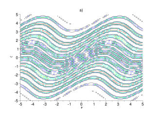
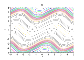
Figure 2: Liouville distribution contour plots: a) without coulombian diffusion, b) with coulombian diffusion $D=0.7$.

                              

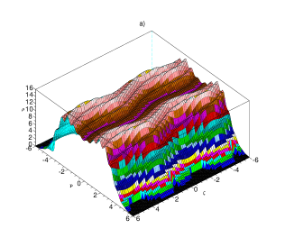
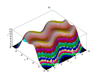
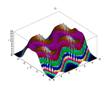
Figure 3: Liouville distribution under the action of the coulombian diffusion ($D=0.7$) for different s values: a) $s=0.06$, b) $s=0.2$, c)$s=0.3$.

The nice feature of the procedure we are adopting is its modularity, which will be further appreciated in the forthcoming section.

III Final Comments

In the introductory section we have expanded the initial distribution, by neglecting the contributions in $A^{2}$. Such an approximation implies that the induced energy modulation is not large compared to the natural e-beam energy spread. However if we relax these assumptions and employ the formalism of generalized Bessel functions Babusci , we can obtain a more general view on the problem under study. It has indeed been shown that two variable Bessel functions can be expressed through the generating function

$$e^{ix\sin(\vartheta)-y(\sin(\vartheta))^{2}}=\sum_{n=-\infty}^{+\infty}e^{in\vartheta}\,_{H}J_{n}(x,y),$$ (22)

$$\,{}_{H}J_{n}(x,y)=\sum_{r=0}^{\infty}\frac{\left(-1\right)^{r}}{2^{n+2r}}\frac{H_{n+2r}(x,y)}{r!(n+r)!},$$

$$H_{n}(x,y)=n!\sum_{r=0}^{n/2}\frac{x^{n-2r}y^{r}}{r!(n-2r)!}$$

where $H_{n}(x,y)$ are two variable Hermite-Kampￜ dￜ Fￜriￜt polynomials Babusci . They are actually understood as belonging to the family of Hermite based functions and are widely exploited to deal with radiation scattering problems Reiss , going beyond the dipole approximation.

It is also worth noting the following operational property Babusci

$$\,{}_{H}J_{n}(x,y)=e^{y\partial_{x}^{2}}J_{n}(x)$$ (23)

which will be used in the following.

The inclusion of the generalized Bessel functions does not change substantively the form of the bunching coefficient, which are obtained from eqs. (9) and (10) by replacing the Bessel function with

$$\,{}_{H}J_{n}(\frac{A_{1}(nB_{1}Ds-ip)}{1+2Ds},\frac{A_{1}^{2}}{1+2Ds})$$

In the second modulator the initial distribution will be provided by the properly modified eq. (9) so that

$$f_{2}(p,\zeta)\cong e^{-B_{2}p\partial_{\zeta}}e^{-A_{2}\sin(\zeta)\partial_{p}}f_{1}(p,\zeta)$$ (24)

which holds if the laser, in the second modulator, is the same of the first. We have removed the $s$ variable because absorbed into the $A$ and $B$ terms. If we use the Bessel function expansion

$$e^{-A_{2}\sin(\zeta)\partial_{p}}=\sum_{n=-\infty}^{\infty}e^{in\zeta}J_{n}(iA_{2}\partial_{p})$$ (25)

we can therefore cast the distribution at the end of the second modulator as

$$f_{2}(p,\zeta)\cong\sum_{n=-\infty}^{\infty}e^{in(\zeta-B_{2}p)}J_{n}(iA_{2}\partial_{p})f_{1}(p,\zeta-B_{2}p)=$$ (26)

$$=\frac{1}{\sqrt{2\pi}}\sum_{n=-\infty}^{\infty}e^{in(\zeta-B_{2}p)}J_{n}(iA_{2}\partial_{p})e^{-\frac{p^{2}}{2}}\sum_{m=-\infty}^{\infty}e^{im(\zeta-(B_{1}-B_{2})p)}J_{m}(-iA_{1}p)$$

By rearranging the indices we end up with

$$f_{2}(p,\zeta)\cong\frac{1}{\sqrt{2\pi}}\sum_{l=-\infty}^{\infty}e^{il\zeta}Q_{l}$$ (27)

$$Q_{l}=\sum_{r=0}^{l}e^{-i(l-r)B_{2}p}J_{l-r}(iA_{2}\partial_{p})e^{-\frac{p^{2}}{2}}e^{-i(l-r)(B_{1}+B_{2})p}J_{r}(-iA_{1}p)$$

According to such a picture the n-th bunching coefficient is characterized by a discrete convolution of the bunching terms of the second modulator on the first.

The effect of the Coulombian diffusion on the distribution (27) can be easily computed, either numerically or analytically. By keeping the lowest order contribution $l=1$ and by approximating the Bessel function as

$$J_{0}(x)\cong 1,\>J_{1}(x)\cong\frac{x}{2}$$

we obtain

$$Q_{1}\cong-\left[\left(\frac{iA_{1}p}{2}\right)+(iA_{2}p)e^{-i(B_{1}+2B_{2})p}-\frac{B_{1}+B_{2}}{2}A_{2}e^{-i(B_{1}+2B_{2})p}\right]e^{-\frac{p^{2}}{2}}.$$ (28)

From the above equation we easily deduce that the Coulombian contribution yields a suppression factor proportional to $e^{-\frac{(B_{1}+2B_{2})^{2}Ds}{1+4Ds}}$ . More in general as also pointed in ref. Stupakov1 the larger is the order of bunching the more significant is the effect of the reduction.

The bunching coefficients vs. s in the presence of diffusion is provided by Fig. 4.

                                 

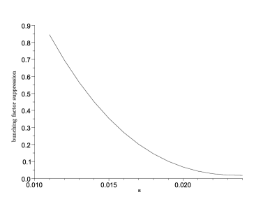
Figure 4: Effect of the coulombian diffusion ( $D=0.7$ ) on the bunching coefficient ( $m=50$) $b_{50}(D)/b_{50}(0)$ vs. s

The formalism we have presented in this paper provides a fairly detailed analysis of how the Coulombian diffusion affect the bunching coefficients in Echo enabled FEL devices. Our treatment is complementary to the seminal contributions of refs. Stupakov1 ; Stupakov2 and confirm, within a more general framework, their conclusions. We believe that the modularity of the methods we have described in this paper offer further opportunities as e. g. that of including in the treatment more complicated arrangements of transport lines and of external fields. The possibility of embedding these procedures with diffusion and damping in storage rings, will be discussed elsewhere.

Appendix

We will discuss here some technical details concerning the solution of the heat equation

$$\partial_{t}F(x,t)=\partial_{x}^{2}F(x,t),$$

$$F(x,0)=x^{n}e^{-x^{2}}$$

which can formally be written as

$$F(x,t)=e^{t\partial_{x}^{2}}(x^{n}e^{-x^{2}})$$

The use of operational methods Babusci yields

$$F(x,t)=(e^{t\partial_{x}^{2}}x^{n}e^{-t\partial_{x}^{2}})e^{t\partial_{x}^{2}}e^{-x^{2}}=$$

$$=(x+2t\partial_{x})^{n}e^{t\partial_{x}^{2}}e^{-x^{2}}.$$

Then by applying the Glaisher and Burchnall Babusci rules, respectively reported below

$$e^{t\partial_{x}^{2}}e^{-x^{2}}=\frac{1}{\sqrt{1+4t}}e^{-\frac{x^{2}}{1+4t}},$$

$$(x+2t\partial_{x})^{n}=\sum_{s=0}^{n}\left(\begin{array}[]{c}n\\ s\end{array}\right)H_{n-s}(x,t)(2t\partial_{x})^{s}$$

provides the solution of our problem in the form

$$F(x,t)=\frac{1}{\sqrt{1+4t}}\sum_{s=0}^{n}\left(\begin{array}[]{c}n\\ s\end{array}\right)H_{n-s}(x,t)(2t\partial_{x})^{s}e^{-\frac{x^{2}}{1+4t}}.$$

The identities Babusci

$$\partial_{x}^{s}e^{-\alpha x^{2}}=(-1)^{s}H_{s}(-2\alpha x,-\alpha),$$

$$H_{n}(\alpha_{1}+\alpha_{2},\beta_{1}+\beta_{2})=\sum_{s=0}^{n}\left(\begin{array}[]{c}n\\ s\end{array}\right)H_{n-s}(\alpha_{1},\beta_{1})H_{s}(\alpha_{2},\beta_{2})$$

finally provide the result

$$F(x,t)=\frac{1}{\sqrt{1+4t}}\sum_{s=0}^{n}\left(\begin{array}[]{c}n\\ s\end{array}\right)H_{n-s}(x,t)H_{s}(-\frac{4xt}{1+4t},-\frac{4t^{2}}{1+4t})e^{-\frac{x^{2}}{1+4t}}=$$

$$=\frac{1}{\sqrt{1+4t}}H_{n}(\frac{x}{1+4t},\frac{t}{1+4t})e^{-\frac{x^{2}}{1+4t}}.$$

It is accordingly evident that for any initial condition such that

$$F(x,0)=g(x)e^{-x^{2}}$$

with

$$g(x)=\sum_{p}a_{p}x^{p}$$

$$F(x,t)=\frac{1}{\sqrt{1+4t}}\sum_{p}a_{p}H_{p}(\frac{x}{1+4t},\frac{t}{1+4t})e^{-\frac{x^{2}}{1+4t}}.$$

References

• (1) G. Stupakov, Phys. Rev.Lett. 102, 074801 (2009).
• (2) G. Stupakov, in Proc. of FEL2011 Conference , Shanghai, China (2011).
• (3) D. Babusci, G. Dattoli, M. Quattromini, E. Sabia, Phys. Rev. E 87, 033202 (2013), (and references therein).
• (4) A. J. Dragt, ’Lie methods for nonlinear dynamics with application to accelerator physics’ University of Maryland (2013).
• (5) D. Babusci, G. Dattoli and M. Delfranco, Lectures on Mathematical Methods for Physics, RT/2010/58/ENEA.
• (6) G. Dattoli, L. Giannessi, A. Torre, JOSA B, 10, 2136 (1993).
• (7) H.R. Reiss, Phys. Rev. A22, 1786 (1980).