Arithmetic Algorithms for Hereditarily Binary Natural Numbers

Abstract

arithmetic computations with giant numbers, hereditary numbering systems, declarative specification of algorithms, compressed number representations, compact representation of large primes

1 Introduction

Number representations have evolved over time from the unary “cave man” representation where one scratch on the wall represented a unit, to the base-n (and in particular base-2) number system, with the remarkable benefit of a logarithmic representation size. Over the last 1000 years, this base-$n$ representation has proved to be unusually resilient, partly because all practical computations could be performed with reasonable efficiency within the notation.

However, when thinking ahead for the next 1000 years, computations with very large numbers are likely to become more and more “natural”, even if for now, they are mostly driven by purely theoretical interests in fields like number theory, computability or multiverse cosmology. Arguably, more practical needs of present and future cryptographic systems might also justify devising alternative numbering systems with higher limits on the size of the numbers with which we can perform tractable computations.

While notations like Knuth’s “up-arrow” knuthUp or tetration are useful in describing very large numbers, they do not provide the ability to actually compute with them – as, for instance, addition or multiplication with a natural number results in a number that cannot be expressed with the notation anymore. More exotic notations like Conway’s surreal numbers surreal involve uncountable cardinalities (they contain real numbers as a subset) and are more useful for modeling game-theoretical algorithms rather than common arithmetic computations.

The novel contribution of this paper is a tree-based numbering system that allows computations with numbers comparable in size with Knuth’s “arrow-up” notation. Moreover, these computations have a worse case complexity that is comparable with the traditional binary numbers, while their best case complexity outperforms binary numbers by an arbitrary tower of exponents factor. Simple operations like successor, multiplication by 2, exponent of 2 are practically constant time and a number of other operations benefit from significant complexity reductions.

For the curious reader, it is basically a hereditary number system goodstein , based on recursively applied run-length compression of a special (bijective) binary digit notation.

A concept of structural complexity is introduced, based on the size of our tree representations and it is shown that several “record holder” large numbers like Mersenne, Cullen, Woodall and Proth primes have unusually small structural complexities.

We have adopted a literate programming style, i.e. the code contained in the paper forms a self-contained Haskell module (tested with ghc 7.6.3), also available as a separate file at http://logic.cse.unt.edu/tarau/research/2013/hbin.hs . Alternatively, a Scala package implementing the same tree-based computations is available from http://code.google.com/p/giant-numbers/. We hope that this will encourage the reader to experiment interactively and validate the technical correctness of our claims. The Appendix contains a quick overview of the subset of Haskell we are using as our executable function notation.

The paper is organized as follows. Section 2 gives some background on bijective base-2 numbers and iterated function applications. Section 3 introduces hereditarily binary numbers. Section 4 describes practically constant time successor and predecessor operations on tree-represented numbers. Section 5 shows an emulation of bijective base-2 with hereditarily binary numbers and section 6 describes novel algorithms for arithmetic operations taking advantage of our number representation. Section 7 defines a concept of structural complexity and studies best and worse cases. Section 8 describes efficient tree-representations of some important number-theoretical entities like Mersenne, Fermat, Proth, Woodall primes. Section 10 discusses related work. Section 11 concludes the paper and discusses future work.

2 Natural numbers as iterated function applications

Natural numbers can be seen as represented by iterated applications of the functions $o(x)=2x+1$ and $i(x)=2x+2$ corresponding the so called bijective base-2 representation sac12 together with the convention that 0 is represented as the empty sequence. As each $n\in\mathbb{N}$ can be seen as a unique composition of these functions we can make this precise as follows:

Definition 1

We call bijective base-2 representation of $n\in\mathbb{N}$ the unique sequence of applications of functions $o$ and $i$ to $\epsilon$ that evaluates to $n$.

With this representation, and denoting the empty sequence $\epsilon$, one obtains $0=\epsilon,1=o~{}\epsilon,2=i~{}\epsilon,3=o(o~{}\epsilon),4=i(o~{}\epsilon),5=o(i~{}\epsilon)$ etc. and the following holds:

$$i(x)=o(x)+1$$ (1)

2.1 Properties of the iterated functions $o^{n}$ and $i^{n}$

Proposition 1

Let $f^{n}$ denote application of function $f$ $n$ times. Let $o(x)=2x+1$ and $i(x)=2x+2$, $s(x)=x+1$ and $s^{\prime}(x)=x-1$. Then $k>0\Rightarrow s(o^{n}(s^{\prime}(k))=k2^{n}$ and $k>1\Rightarrow s(s(i^{n}(s^{\prime}(s^{\prime}(k))))=k2^{n}$. In particular, $s(o^{n}(0))=2^{n}$ and $s(s(i^{n}(0)))=2^{n+1}$.

Proof 2.1.

By induction. Observe that for $n=0,k>0,s(o^{0}(s^{\prime}(k))=k2^{0}$ because $s(s^{\prime}(k)))=k$. Suppose that $P(n):k>0\Rightarrow s(o^{n}(s^{\prime}(k)))=k2^{n}$ holds. Then, assuming $k>0$, P(n+1) follows, given that $s(o^{n+1}(s^{\prime}(k)))=s(o^{n}(o(s^{\prime}(k))))=s(o^{n}(s^{\prime}(2k)))=2k2^{n}=k2^{n+1}$. Similarly, the second part of the proposition also follows by induction on $n$.

The underlying arithmetic identities are:

$$k>0\Rightarrow 1+o^{n}(k-1)=2^{n}k$$ (2)

$$k>1\Rightarrow 2+i^{n}(k-2)=2^{n}k$$ (3)

from where one can deduce

$$o^{n}(k)=2^{n}(k+1)-1$$ (4)

$$i^{n}(k)=2^{n}(k+2)-2$$ (5)

and in particular

$$o^{n}(0)=2^{n}-1$$ (6)

$$i^{n}(0)=2^{n+1}-2$$ (7)

Also, one can directly relate $o^{k}$ and $i^{k}$

$$o^{n}(k)+2^{n}=i^{n}(k)+1$$ (8)

$$i^{n}(k)=o^{n}(k)+o^{n}(0)$$ (9)

$$o^{n}(k+1)=i^{n}(k)+1$$ (10)

2.2 The iterated functions $o^{n}$, $i^{n}$ and their conjugacy results

Results from the theory of iterated functions apply to our operations. The following proposition is proven in iterfun :

Proposition 1.

If $f(x)=ax+b$ with $a\neq 1$, let $x_{0}$ be such that $f(x_{0})=x_{0}$ i.e. $x_{0}={b\over{1-a}}$. Then $f^{n}(x)=x_{0}+(x-x_{0})a^{n}$.

For $a=2,b=1$ and respectively $a=2,b=2$ this provides an alternative proof for proposition 1.

A few properties similar to topological conjugation apply to our functions

Definition 2

We call two functions $f,g$ conjugates through $h$ if $h$ is a bijection such that $g=h^{-1}\circ f\circ h$, where $\circ$ denotes function composition.

Proposition 2.

If $f,g$ are conjugates through $h$ then $f^{n}$ and $g^{n}$ are too, i.e. $g^{n}=h^{-1}\circ{f^{n}}\circ h$.

Proof 2.2.

By induction, using the fact that $h^{-1}\circ h=\lambda x.x=h\circ h^{-1}$.

Proposition 3.

$o^{n}$ and $i^{n}$ are conjugates with respect to $s$ and $s^{\prime}$, i.e. the following 2 identities hold:

$$o^{n}(k)=s(i^{n}(s^{\prime}(k)))$$ (11)

$$i^{n}(k)=s^{\prime}(o^{n}(s(k)))$$ (12)

Proof 2.3.

An immediate consequence of $i=s\circ o$ (by 1) and Prop. 2.

Note also that proposition 1 can be seen as stating that $o^{n}$ is the conjugate of the leftshift operation $l(n,x)=2^{n}x$ through $s(x)=x+1$ (eq. 2) and so is $i^{n}$ through $s\circ s$ (eq. 3).

The following equations relate successor and predecessor to the iterated applications of $o$ and $i$:

$$s(o^{n}(k))=i(o^{s^{\prime}(n)}(k))$$ (13)

$$s(i^{n}(k))=o^{n}(s(k))$$ (14)

$$s^{\prime}(o^{n}(k))=i^{n}(s^{\prime}(k))$$ (15)

$$s^{\prime}(i^{n}(k))=o(i^{s^{\prime}(n)}(k))$$ (16)

By setting $k=2m+1$ in eq. 2 we obtain:

$$1+o^{n}(2m)=2^{n}(2m+1)$$ (17)

As the right side of this equation expresses a bijection between $\mathbb{N}\times\mathbb{N}$ and $\mathbb{N}^{+}$, so does the left side, i.e. the function $c(m,n)=1+o^{n}(2m)$ maps pairs (m,n) to unique values in $\mathbb{N}^{+}$.

Similarly, by setting $k=2m+1$ in eq. 3 we obtain:

$$2+i^{n}(2m-1)=2^{n}(2m+1)$$ (18)

3 Hereditarily binary numbers

3.1 Hereditary Number Systems

Let us observe that conventional number systems, as well as the bijective base-2 numeration system described so far, represent blocks of 0 and 1 digits somewhat naively - one digit for each element of the block. Alternatively, one might think that counting them and representing the resulting counters as binary numbers would be also possible. But then, the same principle could be applied recursively. So instead of representing each block of 0 or 1 digits by as many symbols as the size of the block – essentially a unary representation – one could also encode the number of elements in such a block using a binary representation.

This brings us to the idea of hereditary number systems. At our best knowledge the first instance of such a system is used in goodstein , by iterating the polynomial base-n notation to the exponents used in the notation. We next explore a hereditary number representation that implements the simple idea of representing the number of contiguous 0 or 1 digits in a number, as bijective base-2 numbers, recursively.

3.2 Hereditarily binary numbers as a data type

First, we define a data type for our tree represented natural numbers, that we call hereditarily binary numbers to emphasize that binary rather than unary encoding is recursively used in their representation.

Definition 3

The data type $\mathbb{T}$ of the set of hereditarily binary numbers is defined by the Haskell declaration:

⬇

data T $=$ E $\mid$ V T [T] $\mid$ W T [T] deriving (Eq,Show,Read)

that automatically derives the equality relation “==”, as well as reading and string representation. For shortness, We will call the members of type $\mathbb{T}$ terms. The intuition behind the disjoint union type $\mathbb{T}$ is the following:

• The term E (empty leaf) corresponds to zero

• the term V x xs counts the number x+1 of o applications followed by an alternation of similar counts of i and o applications

• the term W x xs counts the number x+1 of i applications followed by an alternation of similar counts of o and i applications

• the same principle is applied recursively for the counters, until the empty sequence is reached

One can see this process as run-length compressed bijective base-2 numbers, represented as trees with either empty leaves or at least one branch, after applying the encoding recursively.

These trees can be specified in the proof assistant Coq Coq:manual as the type T:

Require Import List.
Inductive T : Type :=
| E : T
| V : T -> list T -> T
| W : T -> list T -> T.

which automatically generates the induction principle:

Coq < Check T_ind.
hbNat_ind
     : forall P : T -> Prop,
       P E ->
       (forall h : T, P h ->
          forall l : list T, P (V h l)) ->
       (forall h : T, P h ->
          forall l : list T, P (W h l)) ->
       forall h : T, P h

Definition 4

The function $n:\mathbb{T}\to\mathbb{N}$ shown in equation 19 defines the unique natural number associated to a term of type $\mathbb{T}$.

$$n(t)=\begin{cases}0&\text{if $t=~{}${\tt E}},\\ 2^{n(x)+1}-1&\text{if $t=~{}${\tt V x []}},\\ {(n(u)+1)}2^{n(x)+1}-1&\text{if $t=~{}${\tt V x (y:xs)} and $u=~{}${\tt W y xs}},\\ 2^{n(x)+2}-2&\text{if $t=~{}${\tt W x []}},\\ {(n(u)+2)}2^{n(x)+1}-1&\text{if $t=~{}${\tt W x (y:xs)} and $u=~{}${\tt V y xs}}.\end{cases}$$ (19)

For instance, the computation of n(W (V E []) [E,E,E])$~{}=42$ expands to $({({({2^{{0}+1}-1}+2)2^{{0}+1}-2}+1)2^{{0}+1}-1}+2)2^{{2^{{0}+1}-1}+1}-2$. The Haskell equivalent of equation (19) is:

⬇

n E $=$ 0

n (V x []) $=$ 2^(n x $+$1)-1

n (V x (y:xs)) $=$ (n u$+$1)$*$2^(n x $+$ 1)-1 where u $=$ W y xs

n (W x []) $=$ 2^(n x$+$2)-2

n (W x (y:xs)) $=$ (n u$+$2)$*$2^(n x $+$ 1)-2 where u $=$ V y xs

The following example illustrates the values associated with the first few natural numbers.

0 = n E
1 = n (V E [])
2 = n (W E [])
3 = n (V (V E []) [])
4 = n (W E [E])
5 = n (V E [E])

Note that a term of the form V x xs represents an odd number $\in\mathbb{N}^{+}$ and a term of the form W x xs represents an even number $\in\mathbb{N}^{+}$. The following holds:

Proposition 4.

$n:\mathbb{T}\to\mathbb{N}$ is a bijection, i.e., each term canonically represents the corresponding natural number.

Proof 3.1.

It follows from the equations 4, 5 by replacing the power of 2 functions with the corresponding iterated applications of $o$ and $i$.

4 Successor (s) and predecessor (s’)

We will now specify successor and predecessor on data type $\mathbb{T}$ through two mutually recursive functions defined in the proof assistant Coq as

Fixpoint s (t:T) :=
match t with
| E => V E nil
| V E nil =>  W E nil
| V E (x::xs) =>  W (s x) xs
| V z xs => W E (s’ z :: xs)
| W z nil => V (s z) nil
| W z (E::nil) => V z (E::nil)
| W z (E::y::ys) => V z (s y::ys)
| W z (x::xs) => V z (E::s’ x::xs)
end
with
s’ (t:T) : T :=
match t with
| V E nil => E
| V z nil => W (s’ z) nil
| V z (E::nil) =>  W z (E::nil)
| V z (E::x::xs) =>  W z (s x::xs)
| V z (x::xs) =>  W z (E::s’ x::xs)
| W E nil => V E nil
| W E (x::xs) => V (s x) xs
| W z xs => V E (s’ z::xs)
| E => E (* Coq wants t total on T *)
end.

Note that our definitions are conforming with Coq’s requirement for automatically guaranteeing termination, i.e. they use only induction on the structure of the terms. Once accepting the definition, Coq allows extraction of equivalent Haskell code, that, in a more human readable form looks as follows:

⬇

s E $=$ V E []

s (V E []) $=$ W E []

s (V E (x:xs)) $=$ W (s x) xs

s (V z xs) $=$ W E (s’ z : xs)

s (W z []) $=$ V (s z) []

s (W z [E]) $=$ V z [E]

s (W z (E:y:ys)) $=$ V z (s y:ys)

s (W z (x:xs)) $=$ V z (E:s’ x:xs)

⬇

s’ (V E []) $=$ E

s’ (V z []) $=$ W (s’ z) []

s’ (V z [E]) $=$ W z [E]

s’ (V z (E:x:xs)) $=$ W z (s x:xs)

s’ (V z (x:xs)) $=$ W z (E:s’ x:xs)

s’ (W E []) $=$ V E []

s’ (W E (x:xs)) $=$ V (s x) xs

s’ (W z xs) $=$ V E (s’ z:xs)

The following holds:

Proposition 5.

Denote $\mathbb{T}^{+}=\mathbb{T}-\{\text{\tt E}\}$. The functions $s:\mathbb{T}\to\mathbb{T}^{+}$ and $s^{\prime}:\mathbb{T}^{+}\to\mathbb{T}$ are inverses.

Proof 4.1.

It follows by structural induction after observing that patterns for V in s correspond one by one to patterns for W in s’ and vice versa.

More generally, it can be proved by structural induction that Peano’s axioms hold and as a result $<\mathbb{T},E,s>$ is a Peano algebra.

Note also that calls to s,s’ in s or s’ happen on terms that are (roughly) logarithmic in the bitsize of their operands. One can therefore assume that their complexity, computed by an iterated logarithm, is practically constant.

5 Emulating the bijective base-2 operations o, $i$

To be of any practical interest, we will need to ensure that our data type $\mathbb{T}$ emulates also binary arithmetic. We will first show that it does, and next we will show that on a number of operations like exponent of 2 or multiplication by an exponent of 2, it significantly lowers complexity.

Intuitively the first step should be easy, as we need to express single applications or “un-applications” of o and i in terms of their iterates encapsulated in the V and W terms.

First we emulate single applications of o and i seen as virtual “constructors” on type data B = Zero | O B | I B.

⬇

o E $=$ V E []

o (V x xs) $=$ V (s x) xs

o (W x xs) $=$ V E (x:xs)

i E $=$ W E []

i (V x xs) $=$ W E (x:xs)

i (W x xs) $=$ W (s x) xs

Next we emulate the corresponding “destructors” that can be seen as “un-applying” a single instance of o or i.

⬇

o’ (V E []) $=$ E

o’ (V E (x:xs)) $=$ W x xs

o’ (V x xs) $=$ V (s’ x) xs

i’ (W E []) $=$ E

i’ (W E (x:xs)) $=$ V x xs

i’ (W x xs) $=$ W (s’ x) xs

Finally the “recognizers” o_ (corresponding to odd numbers) and i_ (corresponding to even numbers) simply detect V and W corresponding to o (and respectively i) being the last function applied.

⬇

o_ (V _ _ ) $=$ True

o_ _ $=$ False

i_ (W _ _ ) $=$ True

i_ _ $=$ False

Note that each of the functions o,o’ and i,i’ call s and s’ on a term that is (roughly) logarithmically smaller. It follows that

Proposition 6.

Assuming s,s’ constant time, o,o’,o,i’ are also constant time.

Definition 5

The function $t:\mathbb{N}\to\mathbb{T}$ defines the unique tree of type $\mathbb{T}$ associated to a natural number as follows:

$$t(x)=\begin{cases}{\tt E}&\text{if $x=~{}${\tt 0}},\\ \text{\tt o}(t({{x-1}\over 2}))&\text{if $x>0$ and $x$ is odd},\\ \text{\tt i}(t({x\over 2}-1))&\text{if $x>0$ and $x$ is even},\\ \end{cases}$$ (20)

We can now define the corresponding Haskell function t:$\mathbb{T}\to\mathbb{N}$ that converts from trees to natural numbers.

Note that pred x=x-1 and div is integer division.

⬇

t 0 $=$ E

t x $\mid$ x$>$0 && odd x $=$ o(t (div (pred x) 2))

t x $\mid$ x$>$0 && even x $=$ i(t (pred (div x 2)))

The following holds:

Proposition 7.

Let id denote $\lambda x.x$ and $\circ$ function composition. Then, on their respective domains

$$t\circ n=id,~{}~{}n\circ t=id$$ (21)

Proof 5.1.

By induction, using the arithmetic formulas defining the two functions.

6 Arithmetic operations

We will now describe algorithms for basic arithmetic operations that take advantage of our number representation.

6.1 A few low complexity operations

Doubling a number db and reversing the db operation (hf) are quite simple, once one remembers that the arithmetic equivalent of function o is $o(x)=2x+1$.

⬇

db $=$ s’ . o

hf $=$ o’ . s

Note that efficient implementations follow directly from our number theoretic observations in section 2.

For instance, as a consequence of proposition 1, the operation exp2, computing an exponent of $2$ , has the following simple definition in terms of s and s’.

⬇

exp2 E $=$ V E []

exp2 x $=$ s (V (s’ x) [])

Proposition 8.

Assuming s,s’ constant time, db,hf and exp2 are also constant time.

Proof 6.1.

It follows by observing that only 2 calls to s,s’,o,o’ are made.

6.2 Simple addition and subtraction algorithms

A simple addition algorithm (add) proceeds by recursing through our emulated bijective base-2 operations o and i.

⬇

simpleAdd E y $=$ y

simpleAdd x E $=$ x

simpleAdd x y $\mid$ o_ x && o_ y $=$

i (simpleAdd (o’ x) (o’ y))

simpleAdd x y $\mid$ o_ x && i_ y $=$

o (s (simpleAdd (o’ x) (i’ y)))

simpleAdd x y $\mid$ i_ x && o_ y $=$

o (s (simpleAdd (i’ x) (o’ y)))

simpleAdd x y $\mid$ i_ x && i_ y $=$

i (s (simpleAdd (i’ x) (i’ y)))

Subtraction is similar.

⬇

simpleSub x E$=$ x

simpleSub y x $\mid$ o_ y && o_ x $=$

s’ (o (simpleSub (o’ y) (o’ x)))

simpleSub y x $\mid$ o_ y && i_ x $=$

s’ (s’ (o (simpleSub (o’ y) (i’ x))))

simpleSub y x $\mid$ i_ y && o_ x $=$

o (simpleSub (i’ y) (o’ x))

simpleSub y x $\mid$ i_ y && i_ x $=$

s’ (o (simpleSub (i’ y) (i’ x)))

The following holds:

Proposition 9.

Assuming that s,s are constant time, the complexity of addition and subtraction is proportional to the bitsize of the smallest of their operands.

Proof 6.2.

The algorithms advance through both their operands with one o’,i’ operation at each call. Therefore the case when one operand is E is reached as soon as the shortest operand is processed.

Note that these simple algorithms do not take advantage of possibly large blocks of $o$ and $i$ operations that could significantly lower complexity on large numbers with such a “regular” structure.

We will derive next versions of these algorithms favoring terms with large contiguous blocks of $o^{n}$ and $i$ applications, on which they will lower complexity to depend on the number of blocks rather than the total number of $o$ and $i$ applications forming the blocks.

Given the recursive, self-similar structure of our trees, as the algorithms mimic the data structures they operate on, we will have to work with a chain of mutually recursive functions. As our focus is to take advantage of large contiguous blocks of $o^{n}$ and $i^{m}$ applications, the algorithms are in uncharted territory and as a result somewhat more intricate than their traditional counterparts.

6.3 Reduced complexity addition and subtraction

We derive more efficient addition and subtraction operations similar to s and s’ that work on one run-length encoded block at a time, rather than by individual o and i steps.

We first define the functions otimes corresponding to $o^{n}(k)$ and itimes corresponding to $i^{n}(k)$.

⬇

otimes E y $=$ y

otimes n E $=$ V (s’ n) []

otimes n (V y ys) $=$ V (add n y) ys

otimes n (W y ys) $=$ V (s’ n) (y:ys)

⬇

itimes E y $=$ y

itimes n E $=$ W (s’ n) []

itimes n (W y ys) $=$ W (add n y) ys

itimes n (V y ys) $=$ W (s’ n) (y:ys)

They are part of a chain of mutually recursive functions as they are already referring to the add function, to be implemented later. Note also that instead of naively iterating, they implement a more efficient algorithm, working “one block at a time”. When detecting that its argument counts a number of applications of o, otimes just increments that count. On the other hand, when the last function applied was i, otimes simply inserts a new count for o operations. A similar process corresponds to itimes. As a result, performance is (roughly) logarithmic rather than linear in terms of the bitsize of argument n. We will also use this property for implementing a low complexity multiplication by exponent of 2 operation.

We will state a number of arithmetic identities on $\mathbb{N}$ involving iterated applications of $o$ and $i$.

Proposition 10.

The following hold:

$$o^{k}(x)+o^{k}(y)=i^{k}(x+y)$$ (22)

$$o^{k}(x)+i^{k}(y)=i^{k}(x)+o^{k}(y)=i^{k}(x+y+1)-1$$ (23)

$$i^{k}(x)+i^{k}(y)=i^{k}(x+y+2)-2$$ (24)

Proof 6.3.

By (4) and (5), we substitute the $2^{k}$-based equivalents of $o^{k}$ and $i^{k}$, then observe that the same reduced forms appear on both sides.

The corresponding Haskell code is:

⬇

oplus k x y $=$ itimes k (add x y)

oiplus k x y $=$ s’ (itimes k (s (add x y)))

iplus k x y $=$ s’ (s’ (itimes k (s (s (add x y)))))

Note the use of add that we will define later as part of a chain of mutually recursive function calls, that together will provide an implementation of the intuitively simple idea: they work on one run-length encoded block at a time. “Efficiency”, in what follows, will be, therefore, conditional to numbers having comparatively few such blocks.

The corresponding identities for subtraction are:

Proposition 11.

$$x>y~{}\Rightarrow~{}o^{k}(x)-o^{k}(y)=o^{k}(x-y-1)+1$$ (25)

$$x>y+1~{}\Rightarrow~{}o^{k}(x)-i^{k}(y)=o^{k}(x-y-2)+2$$ (26)

$$x\geq y~{}\Rightarrow~{}i^{k}(x)-o^{k}(y)=o^{k}(x-y)$$ (27)

$$x>y~{}\Rightarrow~{}i^{k}(x)-i^{k}(y)=o^{k}(x-y-1)+1$$ (28)

Proof 6.4.

By (4) and (5), we substitute the $2^{k}$-based equivalents of $o^{k}$ and $i^{k}$, and observe that the same reduced forms appear on both sides. Note that special cases are handled separately to ensure that subtraction is defined.

The Haskell code, also covering the special cases, is:

⬇

ominus _ x y $\mid$ x $=$$=$ y $=$ E

ominus k x y $=$ s (otimes k (s’ (sub x y)))

iminus _ x y $\mid$ x $=$$=$ y $=$ E

iminus k x y $=$ s (otimes k (s’ (sub x y)))

oiminus k x y $\mid$ x$=$$=$s y $=$ s E

oiminus k x y $\mid$ x $=$$=$ s (s y) $=$ s (exp2 k)

oiminus k x y $=$ s (s (otimes k (s’ (s’ (sub x y)))))

iominus k x y $=$ otimes k (sub x y)

Note the reference to sub, to be defined later, which is also part of the mutually recursive chain of operations.

The next two functions extract the iterated applications of $o^{n}$ and respectively $i^{n}$ from V and W terms:

⬇

osplit (V x []) $=$ (x,E )

osplit (V x (y:xs)) $=$ (x,W y xs)

isplit (W x []) $=$ (x,E )

isplit (W x (y:xs)) $=$ (x,V y xs)

We are now ready for defining addition. The base cases are the same as for simpleAdd:

⬇

add E y $=$ y

add x E $=$ x

In the case when both terms represent odd numbers, we apply the identity (22), after extracting the iterated applications of $o$ as a and b with the function osplit.

⬇

add x y $\mid$o_ x && o_ y $=$ f (cmp a b) where

(a,as) $=$ osplit x

(b,bs) $=$ osplit y

f EQ $=$ oplus (s a) as bs

f GT $=$ oplus (s b) (otimes (sub a b) as) bs

f LT $=$ oplus (s a) as (otimes (sub b a) bs)

In the case when the first term is odd and the second even, we apply the identity (23), after extracting the iterated application of $o$ and $i$ as a and b.

⬇

add x y $\mid$o_ x && i_ y $=$ f (cmp a b) where

(a,as) $=$ osplit x

(b,bs) $=$ isplit y

f EQ $=$ oiplus (s a) as bs

f GT $=$ oiplus (s b) (otimes (sub a b) as) bs

f LT $=$ oiplus (s a) as (itimes (sub b a) bs)

In the case when the first term is even and the second odd, we apply the identity (23), after extracting the iterated applications of $i$ and $o$ as, respectively, a and b.

⬇

add x y $\mid$i_ x && o_ y $=$ f (cmp a b) where

(a,as) $=$ isplit x

(b,bs) $=$ osplit y

f EQ $=$ oiplus (s a) as bs

f GT $=$ oiplus (s b) (itimes (sub a b) as) bs

f LT $=$ oiplus (s a) as (otimes (sub b a) bs)

In the case when both terms represent even numbers, we apply the identity (24), after extracting the iterated application of $i$ as a and b.

⬇

add x y $\mid$i_ x && i_ y $=$ f (cmp a b) where

(a,as) $=$ isplit x

(b,bs) $=$ isplit y

f EQ $=$ iplus (s a) as bs

f GT $=$ iplus (s b) (itimes (sub a b) as) bs

f LT $=$ iplus (s a) as (itimes (sub b a) bs)

Note the presence of the comparison operation cmp, to be defined later, also part of our chain of mutually recursive operations. Note also the local function f that in each case ensures that a block of the same size is extracted, depending on which of the two operands a or b is larger. The code for the subtraction function sub is similar:

⬇

sub x E $=$ x

sub x y $\mid$ o_ x && o_ y $=$ f (cmp a b) where

(a,as) $=$ osplit x

(b,bs) $=$ osplit y

f EQ $=$ ominus (s a) as bs

f GT $=$ ominus (s b) (otimes (sub a b) as) bs

f LT $=$ ominus (s a) as (otimes (sub b a) bs)

In the case when both terms represent odd numbers, we apply the identity (25), after extracting the iterated applications of $o$ as a and b. For the other cases, we use, respectively, the identities 26, 27 and 28:

⬇

sub x y $\mid$o_ x && i_ y $=$ f (cmp a b) where

(a,as) $=$ osplit x

(b,bs) $=$ isplit y

f EQ $=$ oiminus (s a) as bs

f GT $=$ oiminus (s b) (otimes (sub a b) as) bs

f LT $=$ oiminus (s a) as (itimes (sub b a) bs)

sub x y $\mid$i_ x && o_ y $=$ f (cmp a b) where

(a,as) $=$ isplit x

(b,bs) $=$ osplit y

f EQ $=$ iominus (s a) as bs

f GT $=$ iominus (s b) (itimes (sub a b) as) bs

f _ $=$ iominus (s a) as (otimes (sub b a) bs)

sub x y $\mid$i_ x && i_ y $=$ f (cmp a b) where

(a,as) $=$ isplit x

(b,bs) $=$ isplit y

f EQ $=$ iminus (s a) as bs

f GT $=$ iminus (s b) (itimes (sub a b) as) bs

f LT $=$ iminus (s a) as (itimes (sub b a) bs)

6.4 Defining a total order: comparison

The comparison operation cmp provides a total order (isomorphic to that on $\mathbb{N}$) on our type $\mathbb{T}$. It relies on bitsize computing the number of applications of $o$ and $i$ constructing a term in $\mathbb{T}$. It is part of our mutually recursive functions, to be defined later.

We first observe that only terms of the same bitsize need detailed comparison, otherwise the relation between their bitsizes is enough, recursively. More precisely, the following holds:

Proposition 12.

Let bitsize count the number of applications of $o$ and $i$ operations on a bijective base-2 number. Then bitsize$(x)<$bitsize$(y)\Rightarrow x<y$.

Proof 6.5.

Observe that their lexicographic enumeration ensures that the bitsize of bijective base-2 numbers is a non-decreasing function.

⬇

cmp E E $=$ EQ

cmp E _ $=$ LT

cmp _ E $=$ GT

cmp x y $\mid$ x’ $/$$=$ y’ $=$ cmp x’ y’ where

x’ $=$ bitsize x

y’ $=$ bitsize y

cmp x y $=$

compBigFirst (reversedDual x) (reversedDual y)

The function compBigFirst compares two terms known to have the same bitsize. It works on reversed (big digit first) variants, computed by reversedDual and it takes advantage of the block structure using the following proposition:

Proposition 13.

Assuming two terms of the same bitsizes, the one starting with $i$ is larger than one starting with $o$.

Proof 6.6.

Observe that “big digit first” numbers are lexicographically ordered with $o<i$.

As a consequence, cmp only recurses when identical blocks head the sequence of blocks, otherwise it infers the LT or GT relation.

⬇

compBigFirst E E $=$ EQ

compBigFirst x y $\mid$ o_ x && o_ y $=$ f (cmp a b) where

(a,c) $=$ osplit x

(b,d) $=$ osplit y

f EQ $=$ compBigFirst c d

f LT $=$ GT

f GT $=$ LT

compBigFirst x y $\mid$ i_ x && i_ y $=$ f (cmp a b) where

(a,c) $=$ isplit x

(b,d) $=$ isplit y

f EQ $=$ compBigFirst c d

f other $=$ other

compBigFirst x y $\mid$ o_ x && i_ y $=$ LT

compBigFirst x y $\mid$ i_ x && o_ y $=$ GT

The function reversedDual reverses the order of application of the $o$ and $i$ operations to a “biggest digit first” order. For this, it only needs to reverse the order of the alternative blocks of $o^{k}$ and $i^{l}$. It uses the function len to compute the number of these blocks and infer that if odd, the last block is the same as the first and otherwise it is its alternate.

⬇

reversedDual E $=$ E

reversedDual (V x xs) $=$ f (len (y:ys)) where

(y:ys) $=$ reverse (x:xs)

f l $\mid$ o_ l $=$ V y ys

f l $\mid$ i_ l $=$ W y ys

reversedDual (W x xs) $=$ f (len (y:ys)) where

(y:ys) $=$ reverse (x:xs)

f l $\mid$ o_ l $=$ W y ys

f l $\mid$ i_ l $=$ V y ys

⬇

len [] $=$ E

len (_:xs) $=$ s (len xs)

And based on cmp, one can define the minimum min2, maximum max2 the absolute value of the difference absdif functions as follows:

⬇

min2 x y $=$ if LT$=$$=$cmp x y then x else y

max2 x y $=$ if LT$=$$=$cmp x y then y else x

absdif x y $=$ if LT $=$$=$ cmp x y then sub y x else sub x y

6.5 Computing dual and bitsize

The function dual flips o and i operations for a natural number seen as written in bijective base 2. Note that with our tree representation it is constant time, as it simply flips once the constructors V and W.

⬇

dual E $=$ E

dual (V x xs) $=$ W x xs

dual (W x xs) $=$ V x xs

The function bitsize computes the number of applications of the o and i operations. It works by summing up (using Haskell’s foldr) the counts of o and i operations composing a tree-represented natural number.

⬇

bitsize E $=$ E

bitsize (V x xs) $=$ s (foldr add1 x xs)

bitsize (W x xs) $=$ s (foldr add1 x xs)

add1 x y $=$ s (add x y)

Note that bitsize also provides an efficient implementation of the integer $log_{2}$ operation ilog2.

⬇

ilog2 x $=$ bitsize (s’ x)

6.6 Fast multiplication by an exponent of 2

The function leftshiftBy operation uses the fact that repeated application of the o operation (otimes) , provides an efficient implementation of multiplication with an exponent of 2.

⬇

leftshiftBy _ E $=$ E

leftshiftBy n k $=$ s (otimes n (s’ k))

The following holds:

Proposition 14.

Assuming s,s’ constant time, leftshiftBy is (roughly) logarithmic in the bitsize of its arguments.

Proof 6.7.

it follows by observing that at most one addition on data logarithmic in the bitsize of the operands is performed.

6.7 Fast division by an exponent of 2

Division by an exponent of 2 (equivalent to the rightshift operation is more intricate. It takes advantage of identities (4) and (5) in a way that is similar to add and sub. First, the function toShift transforms the outermost block of $o^{m}$ or $i^{m}$ applications to to a multiplication of the form $k2^{m}$. It also remembers if it had $o^{m}$ or $i^{m}$, as the first component of the triplet it returns. Note that, as a result, the operation is actually reversible.

⬇

toShift x $\mid$ o_ x $=$ (o E,m,k) where

(a,b) $=$ osplit x

m $=$ s a

k $=$ s b

toShift x $\mid$ i_ x $=$ (i E,m,k) where

(a,b) $=$ isplit x

m $=$ s a

k $=$ s (s b)

Next the function rightshiftBy goes over its argument k one block at a time, by comparing the size of the block and its argument m that is decremented after each block by the size of the block. The local function f handles the details, according to the nature of the block ($o^{m}$ or $i^{m}$), and stops when the argument is exhausted. More precisely, based on the result EQ, LT, GT of the comparison, as well on the type of block (as recognized by o_ p and i_ p), it applies back otimes or itimes when the block is larger than the value of m. Otherwise, it calls itself with the value of m reduced by the size to the block as its first argument.

⬇

rightshiftBy _ E $=$ E

rightshiftBy m k $=$ f (cmp m a) where

(p,a,b) $=$ toShift k

f EQ $\mid$ o_ p $=$ sub b p

f EQ $\mid$ i_ p $=$ s (sub b p)

f LT $\mid$ o_ p $=$ otimes (sub a m) (sub b p)

f LT $\mid$ i_ p $=$ s (itimes (sub a m) (sub b p))

f GT $=$ rightshiftBy (sub m a) b

The following example illustrates the fact that rightShiftBy inverts the result ofleftshiftBy on a very large number.

*HBin> s’ (exp2 (t 100000))
V (V (W E [E]) [E,E,E,E,V E [],V (V E []) [],E]) []
*HBin> leftshiftBy (t 1000) it
W E [W (W E []) [V E [],V (V E []) []],W (W E [E])
    [V E [],E,E,V E [],V (V E []) [],E]]
*HBin> rightshiftBy (t 1000) it
V (V (W E [E]) [E,E,E,E,V E [],V (V E []) [],E]) []

6.8 Reduced complexity general multiplication

Devising a similar optimization as for add and sub for multiplication is actually easier.

Proposition 15.

The following holds:

$$o^{n}(a)o^{m}(b)=o^{n+m}(ab+a+b)-o^{n}(a)-o^{m}(b)$$ (29)

Proof 6.8.

By (4), we can expand and then reduce: $o^{n}(a)o^{m}(b)=(2^{n}(a+1)-1)(2^{m}(b+1)-1)=2^{n+m}(a+1)(b+1)-(2^{n}(a+1)+2^{m}(b+1)+1=2^{n+m}(a+1)(b+1)-1-(2^{n}(a+1)-1+2^{m}(b+1)-1+2)+2=o^{n+m}(ab+a+b+1)-(o^{n}(a)+o^{m}(b))-2+2=o^{n+m}(ab+a+b)-o^{n}(a)-o^{m}(b)$

The corresponding Haskell code starts with the obvious base cases:

⬇

mul _ E $=$ E

mul E _ $=$ E

When both terms represent odd numbers we apply the identity (29):

⬇

mul x y $\mid$ o_ x && o_ y $=$ r2 where

(n,a) $=$ osplit x

(m,b) $=$ osplit y

p1 $=$ add (mul a b) (add a b)

p2 $=$ otimes (add (s n) (s m)) p1

r1 $=$ sub p2 x

r2 $=$ sub r1 y

The other cases are reduced to the previous one by using the identity $i=s.o$.

⬇

mul x y $\mid$ o_ x && i_ y $=$ add x (mul x (s’ y))

mul x y $\mid$ i_ x && o_ y $=$ add y (mul (s’ x) y)

mul x y $\mid$ i_ x && i_ y $=$

s (add (add x’ y’) (mul x’ y’)) where

x’$=$s’ x

y’$=$s’ y

Note that when the operands are composed of large blocks of alternating $o^{n}$ and $i^{m}$ applications, the algorithm is quite efficient as it works (roughly) in time proportional to the number of blocks rather than the number of digits. The following example illustrates a blend of arithmetic operations benefiting from complexity reductions on giant tree-represented numbers:

*HBin> let term1 = sub (exp2 (exp2
                    (t 12345))) (exp2 (t 6789))
*HBin> let term2 = add (exp2 (exp2 (t 123)))
                    (exp2 (t 456789))
*HBin> ilog2 (ilog2 (mul term1 term2))
V E [E,E,W E [],V E [E],E]
*HBin> n it
12345

This opens a new world where arithmetic operations are not limited by the size of their operands, but only by their “structural complexity”. We will make this concept more precise in section 7.

6.9 Power

We first specialize our multiplication for a slightly faster squaring operation, using the identity:

$$(o^{n}(a))^{2}=o^{2n}(a^{2}+2a)-2o^{n}(a)$$ (30)

⬇

square E $=$ E

square x $\mid$ o_ x $=$ r where

(n,a) $=$ osplit x

p1 $=$ add (square a) (db a)

p2 $=$ otimes (i n) p1

r $=$ sub p2 (db x)

square x$\mid$ i_ x $=$ s (add (db x’) (square x’)) where

x’ $=$ s’ x

We can implement a simple but fairly efficient “ power by squaring” operation for $x^{y}$ as follows:

⬇

pow _ E $=$ V E []

pow x y $\mid$ o_ y $=$ mul x (pow (square x) (o’ y))

pow x y $\mid$ i_ y $=$ mul x2 (pow x2 (i’ y)) where

x2 $=$ square x

It works well with fairly large numbers, by also benefiting from efficiency of multiplication on terms with large blocks of $o^{n}$ and $o^{m}$ applications:

*HBin> n (bitsize (pow (t 2014) (t 100)))
1097
*HBin> pow (t 32) (t 10000000)
W E [W (W (V E []) []) [W E [E],
  V (V E []) [],E,E,E,W E [E],E]]

7 Structural complexity

As a measure of structural complexity we define the function tsize that counts the nodes of a tree of type $\mathbb{T}$ (except the root).

⬇

tsize E $=$ E

tsize (V x xs) $=$ foldr add1 E (map tsize (x:xs))

tsize (W x xs) $=$ foldr add1 E (map tsize (x:xs))

It corresponds to the function $c:\mathbb{T}\to\mathbb{N}$ defined as follows:

$$c(t)=\begin{cases}0&\text{if $\text{\tt t}=~{}$0},\\ \sum_{y\in(\text{\tt x:xs})}{(1+ts(y))}&\text{if t = \text{\tt V x xs}},\\ \sum_{y\in(\text{\tt x:xs})}{(1+ts(y))}&\text{if t = \text{\tt W x xs}}.\end{cases}$$ (31)

The following holds:

Proposition 16.

For all terms $t\in\mathbb{T}$, tsize t $\leq$ bitsize t.

Proof 7.1.

By induction on the structure of $t$, by observing that the two functions have similar definitions and corresponding calls to tsize return terms assumed smaller than those of bitsize.

The following example illustrates their use:

*HBin> map (n.tsize.t) [0,100,1000,10000]
[0,6,8,10]
*HBin> map (n.bitsize.t) [0,100,1000,10000]
[0,6,9,13]

*HBin> map (n.tsize.t) [2^16,2^32,2^64,2^256]
[4,5,5,5]
*HBin> map (n.bitsize.t) [2^16,2^32,2^64,2^256]
[16,32,64,256]

Figure 1 shows the reductions in structural complexity compared with bitsize for an initial interval of $\mathbb{N}$.

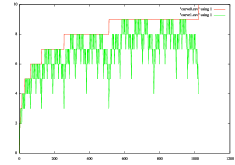
Figure 1: Structural complexity (yellow line) bounded by bitsize (red line) from $0$ to $2^{10}-1$

After defining the function iterated that applies f k times

⬇

iterated f E x $=$ x

iterated f k x $=$ f (iterated f (s’ k) x)

we can exhibit a best case

⬇

bestCase k $=$ s’ (iterated exp2 k E)

and a worse case

⬇

worseCase k $=$ iterated (i.o) k E

The following examples illustrate these functions:

*HBin> bestCase (t 5)
V (V (V (V E []) []) []) []
*HBin> n it
65535
*HBin> bestCase (t 5)
V (V (V (V E []) []) []) []
*HBin> n (bitsize (bestCase (t 5)))
16
*HBin> n (tsize (bestCase (t 5)))
4

*HBin> worseCase (t 5)
W E [E,E,E,E,E,E,E,E,E]
*HBin> n it
1364
*HBin> n (bitsize (worseCase (t 5)))
10
*HBin> n (tsize (worseCase (t 5)))
10

The function bestCase computes the iterated exponent of 2 (tetration) and then applies the predecessor s’ to it. A simple closed formula can also be found for worseCase:

Proposition 17.

The function worseCase k computes the value in $\mathbb{T}$ corresponding to the value ${{4(4^{k}-1)}\over 3}\in\mathbb{N}$.

Proof 7.2.

By induction or by applying the iterated function formula to $f(x)=i(o(x)))=2(2x+1)+2=4(x+1)$.

The average space-complexity of the representation is related to the average length of the integer partitions of the bitsize of a number part99 . Intuitively, the shorter the partition in alternative blocks of $o$ and $i$ applications, the more significant the compression is, but the exact study, given the recursive application of run-length encoding, is likely to be quite intricate.

Note also that our concept of structural complexity is only a weak approximation of Kolmogorov complexity vitanyi . For instance, the reader might notice that our worse case example is computable by a program of relatively small size. However, as bitsize is an upper limit to tsize, we can be sure that we are within constant factors from the corresponding bitstring computations, even on random data of high Kolmogorov complexity.

Note also that an alternative concept of structural complexity can be defined by considering the (vertices+edges) size of the DAG obtained by folding together identical subtrees. We will use such DAGs in section 8 to more compactly visualize large tree-represented numbers.

As section 8 will illustrate it, several interesting number theoretical entities that hold current records in various categories have very low structural complexities, contrasting to gigantic bitsizes.

8 Efficient representation of some important number-theoretical entities

Let’s first observe that Fermat, Mersenne and perfect numbers have all compact expressions with our tree representation of type $\mathbb{T}$.

⬇

fermat n $=$ s (exp2 (exp2 n))

mersenne p $=$ s’ (exp2 p)

perfect p $=$ s (V q [q]) where q $=$ s’ (s’ p)

*HBin> mersenne 127
170141183460469231731687303715884105727
*HBin> mersenne (t 127)
V (W (V E [E]) []) []

The largest known prime number, found by the GIMPS distributed computing project gimps in January 2013 is the 48-th Mersenne prime = $2^{57885161}-1$ (with possibly smaller Mersenne primes below it). It is defined in Haskell as follows:

⬇

-- exponent of the 48-th known Mersenne prime

prime48 $=$ 57885161

-- the actual Mersenne prime

mersenne48 $=$ s’ (exp2 (t prime48))

While it has a bit-size of 57885161, its compressed tree representation is rather small:

*HBin> mersenne48
V (W E [V E [],E,E,V (V E []) [],
   W E [E],E,E,V E [],V E [],W E [],E,E]) []

The equivalent DAG representation of the 48-th Mersenne prime, shown in Figure 2, has only 7 shared nodes and structural complexity 22. Note that the empty leaf node is marked with the letter T.

Figure 2: Largest known prime number discovered in January 2013: the 48-th Mersenne prime, represented as a DAG

It is interesting to note that similar compact representations can also be derived for perfect numbers. For instance, the largest known perfect number, derived from the largest known Mersenne prime as $2^{57885161-1}(2^{57885161}-1)$, (involving only 8 shared nodes and structural complexity 43) is:

⬇

perfect48 $=$ perfect (t prime48)

Fig. 3 shows the DAG representation of the largest known perfect number, derived from Mersenne number 48.

Figure 3: Largest known perfect number in January 2013

Similarly, the largest Fermat number that has been factored so far, $F_{11}=2^{2^{11}}+1$ is compactly represented as

*HBin> fermat (t 11)
V E [E,V E [W E [V E []]]]

with structural complexity 8. By contrast, its (bijective base-2) binary representation consists of 2048 digits.

Some other very large primes that are not Mersenne numbers also have compact representations.

The generalized Fermat prime $27653*2^{9167433}+1$, (currently the 15-the largest prime number) computed as a tree is:

⬇

genFermatPrime $=$ s (leftshiftBy n k) where

n $=$ t (9167433::Integer)

k $=$ t (27653::Integer)

*HBin> genFermatPrime
V E [E,W (W E []) [W E [],E,
  V E [],E,W E [],W E [E],E,E,W E []],
  E,E,E,W (V E []) [],V E [],E,E]

Figure 4 shows the DAG representation of this generalized Fermat prime with 7 shared nodes and structural complexity 30.

Figure 4: Generalized Fermat prime

The largest known Cullen prime $6679881*2^{6679881}+1$ computed as tree (with 6 shared nodes and structural complexity 43) is:

⬇

cullenPrime $=$ s (leftshiftBy n n) where

n $=$ t (6679881::Integer)

*HBin> cullenPrime
V E [E,W (W E []) [W E [],E,E,E,E,V E [],E,
  V (V E []) [],E,E,V E [],E],E,V E [],E,V E [],
  E,E,E,E,V E [],E,V (V E []) [],E,E,V E [],E]

Figure 5 shows the DAG representation of this Cullen prime.

Figure 5: largest known Cullen prime

The largest known Woodall prime $3752948*2^{3752948}-1$ computed as a tree (with 6 shared nodes and structural complexity 33) is:

⬇

woodallPrime $=$ s’ (leftshiftBy n n) where

n $=$ t (3752948::Integer)

*HBin> woodallPrime
V (V E [V E [],E,V E [E],V (V E []) [],
 E,E,E,V E [],V E []]) [E,E,V E [E],
 V (V E []) [],E,E,E,V E [],V E []]

Figure 6 shows the DAG representation of this Woodall prime.

Figure 6: Largest known Woodall prime

The largest known Proth prime $19249*2^{13018586}+1$ computed as a tree is:

⬇

prothPrime $=$ s (leftshiftBy n k) where

n $=$ t (13018586::Integer)

k $=$ t (19249::Integer)

*HBin> prothPrime
V E [E,V (W E []) [V E [],E,W E [],E,E,
  V E [],E,E,E,E,V E [],W E [],E],E,W E [],
  V E [],V E [],V E [],E,E,V E []]

Figure 7 shows the DAG representation of this Proth prime, the largest non-Mersenne prime known by March 2013 with 5 shared nodes and structural complexity 36.

Figure 7: Largest known Proth prime

The largest known Sophie Germain prime $18543637900515*2^{666667}-1$ computed as a tree (with 6 shared nodes and structural complexity 56) is:

⬇

sophieGermainPrime $=$ s’ (leftshiftBy n k) where

n $=$ t (666667::Integer)

k $=$ t (18543637900515::Integer)

*HBin> sophieGermainPrime
V (W (V E []) [E,E,E,E,V (V E []) [],V E [],E,
   E,W E [],E,E]) [V E [],W E [],W E [],V E [],
   V E [],E,E,V E [],V E [],V E [],V (V E [])
   [],E,V E [],V (V E []) [],V E [],E,W E [],E,
   V E [],V (V E []) []]

Figure 8 shows the DAG representation of this prime.

Figure 8: Largest known Sophie Germain prime

The largest known twin primes $3756801695685*2^{666669}\pm 1$ computed as a pair of trees (with 7 shared nodes both and structural complexities of 54 and 56) are:

⬇

twinPrimes $=$ (s’ m,s m) where

n $=$ t (666669::Integer)

k $=$ t (3756801695685::Integer)

m $=$ leftshiftBy n k

*HBin> fst twinPrimes
V (W E [E,V E [],E,E,V (V E []) [],
   V E [],E,E,W E [],E,E])
   [E,E,E,W E [],W (V E []) [],V E [],E,V E [],
   E,E,E,E,V E [],E,E,
   V E [],V E [],E,E,E,E,E,E,E,V E [],E,E]
*HBin> snd twinPrimes
V E [E,W (V E []) [E,E,E,E,V (V E []) [],
  V E [],E,E,W E [],E,E],E,E,E,
  W E [],W (V E []) [],V E [],E,V E [],
  E,E,E,E,V E [],E,E,V E [],
  V E [],E,E,E,E,E,E,E,V E [],E,E]

Figures 9 and 10 show the DAG representation of these twin primes.

Figure 9: Largest known twin prime 1

Figure 10: Largest known twin prime 2

One can appreciate the succinctness of our representations, given that all these numbers have hundreds of thousands or millions of decimal digits. An interesting challenge would be to (re)focus on discovering primes with significantly larger structural complexity then the current record holders by bitsize.

More importantly, as the following examples illustrate it, computations like addition, subtraction and multiplication of such numbers are possible:

*HBin> sub genFermatPrime (t 2014)
V (V E []) [E,V E [],E,W E [E],V E [W E [E],
  W E [],E,W E [],W E [E],E,E,W E []],V E [],
  E,W (V E []) [],V E [],E,E]
*HBin> bitsize (sub prothPrime (t 1234567890))
W E [V E [],E,E,V (V E []) [],E,E,
  V E [],E,E,E,E,V E [],W E [],E]
*HBin> tsize (exp2 (exp2 mersenne48))
V E [E,E,E]
*HBin> tsize(leftshiftBy mersenne48 mersenne48)
V E [W E [],E]
*HBin> add (t 2) (fst twinPrimes) ==
           (snd twinPrimes)
True
*HBin> ilog2 (ilog2 (mul prothPrime cullenPrime))
W E [V E [],E]
*HBin> n it
24

9 Computing the Collatz/Syracuse sequence for huge numbers

As an interesting application, that achieves something one cannot do with ordinary Integers is to explore the behavior of interesting conjectures in the new world of numbers limited not by their sizes but by their structural complexity. The Collatz conjecture states that the function

$$collatz(x)=\begin{cases}x\over 2&\text{if $x$ is even},\\ 3x+1&\text{if $x$ is odd}.\\ \end{cases}$$ (32)

reaches $1$ after a finite number of iterations. An equivalent formulation, by grouping together all the division by 2 steps, is the function:

$$collatz^{\prime}(x)=\begin{cases}x\over 2^{\nu_{2}(x)}&\text{if $x$ is even},\\ 3x+1&\text{if $x$ is odd}.\\ \end{cases}$$ (33)

where $\nu_{2}(x)$ denotes the dyadic valuation of x, i.e., the largest exponent of 2 that divides x. One step further, the syracuse function is defined as the odd integer $k^{\prime}$ such that $n=3k+1=2^{\nu(n)}k^{\prime}$. One more step further, by writing $k^{\prime}=2m+1$ we get a function that associates $k\in\mathbb{N}$ to $m\in\mathbb{N}$.

The function tl computes efficiently the equivalent of

$$tl(k)={{{k\over 2^{\nu_{2}(k)}}-1}\over 2}$$ (34)

⬇

tl n $\mid$ o_ n $=$ o’ n

tl n $\mid$ i_ n $=$ f xs where

V _ xs $=$ s’ n

f [] $=$ E

f (y:ys) $=$ s (i’ (W y ys))

Then our variant of the syracuse function corresponds to

$$syracuse(n)=tl(3n+2)$$ (35)

which we can code efficiently as

⬇

syracuse n $=$ tl (add n (i n))

The function nsyr computes the iterates of this function, until (possibly) stopping:

⬇

nsyr E $=$ [E]

nsyr n $=$ n : nsyr (syracuse n)

It is easy to see that the Collatz conjecture is true if and only if nsyr terminates for all $n$, as illustrated by the following example:

*HBin> map n (nsyr (t 2014))
[2014,755,1133,1700,1275,1913,2870,1076,807,
   1211,1817,2726,1022,383,575,863,1295,1943,
   2915,4373,6560,4920,3690,86,32,24,18,3,5,
   8,6,2,0]

The next examples will show that computations for nsyr can be efficiently carried out for numbers that with traditional bitstring notations would easily overflow even the memory of a computer using as transistors all the atoms in the known universe.

The following examples illustrate this:

map (n.tsize) (take 1000 (nsyr mersenne48))
[22,22,24,26,27,28,...,1292,1313,1335,1353]

As one can see, the structural complexity is growing progressively, but that our tree-numbers have no trouble with the computations.

*HBin> map (n.tsize)
        (take 1000 (nsyr mersenne48))
[22,22,24,26,27,28,...,1292,1313,1335,1353]

Moreover, we can keep going up with a tower of 3 exponents. Interestingly, it results in a fairly small increase in structural complexity over the first 1000 terms.

*HBin> map (n.tsize) (take 1000
        (nsyr (exp2 (exp2 (exp2 mersenne48)))))
[26,33,36,37,40,42,...,1313,1335,1358,1375]

While we did not tried to wait out the termination of the execution for Mersenne number 48 we, have computed nsyr for the record holder from 1952, which is still much larger than the values (up to $5\times 2^{60}$) for which the conjecture has been confirmed true. Figure 11 shows the structural complexity curve for the “hailstone sequence” associated by the function nsyr to the 15-th Mersenne prime, $2^{1279}-1$

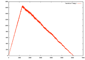
Figure 11: Structural complexity curve for nsyr on $2^{1279}-1$

As an interesting fact, possibly unknown so far, one might notice the abrupt phase transition that, based on our experiments, seem to characterize the behavior of this function, when starting with very large numbers of relatively small structural complexity.

And finally something we are quite sure has never been computed before, we can also start with a tower of exponents 100 levels tall:

*HBin> take 1000 (map(n.tsize)(nsyr (bestCase (t 100))))
[99,99,197,293,294,296,299,299,...,1569,1591,1614,1632]

10 Related work

We will briefly describe here some related work that has inspired and facilitated this line of research and will help to put our past contributions and planned developments in context.

Several notations for very large numbers have been invented in the past. Examples include Knuth’s arrow-up notation knuthUp covering operations like the tetration (a notation for towers of exponents). In contrast to our tree-based natural numbers, such notations are not closed under addition and multiplication, and consequently they cannot be used as a replacement for ordinary binary or decimal numbers.

The first instance of a hereditary number system, at our best knowledge, occurs in the proof of Goodstein’s theorem goodstein , where replacement of finite numbers on a tree’s branches by the ordinal $\omega$ allows him to prove that a “hailstone sequence” visiting arbitrarily large numbers eventually turns around and terminates.

Like our trees of type $\mathbb{T}$, Conway’s surreal numbers surreal can also be seen as inductively constructed trees. While our focus is on efficient large natural number arithmetic and sparse set representations, surreal numbers model games, transfinite ordinals and generalizations of real numbers.

Numeration systems on regular languages have been studied recently, e.g. in Rigo2001469 and specific instances of them are also known as bijective base-k numbers. Arithmetic packages similar to our bijective base-2 view of arithmetic operations are part of libraries of proof assistants like Coq Coq:manual .

Arithmetic computations based on recursive data types like the free magma of binary trees (isomorphic to the context-free language of balanced parentheses) are described in sac12 , where they are seen as Gödel’s System T types, as well as combinator application trees. In ppdp10tarau a type class mechanism is used to express computations on hereditarily finite sets and hereditarily finite functions. In vu09 integer decision diagrams are introduced providing a compressed representation for sparse integers, sets and various other data types.

11 Conclusion and future work

We have provided in the form of a literate Haskell program a declarative specification of a tree-based number system. Our emphasis here was on the correctness and the theoretical complexity bounds of our operations rather than the packaging in a form that would compete with a C-based arbitrary size integer package like GMP. We have also ensured that our algorithms are as simple as possible and we have closely correlated our Haskell code with the formulas describing the corresponding arithmetical properties. As the algorithms involved are all novel and we have explored genuinely uncharted territory, we are not considering this literate program a functional pearl, as we are by no means focusing on polishing known results, but rather on using the niceties of functional programming to model new concepts. For instance, our algorithms rely on properties of blocks of iterated applications of functions rather than the “digits as coefficients of polynomials” view of traditional numbering systems. While the rules are often more complex, restricting our code to a purely declarative subset of functional programming made managing a fairly intricate network of mutually recursive dependencies much easier.

We have shown that some interesting number-theoretical entities like Fermat and perfect numbers, and the largest known Mersenne, Proth, Cullen, Sophie Germain and twin primes have compact representations with our tree-based numbers. One may observe their common feature: they are all represented in terms of exponents of 2, successor/predecessor and specialized multiplication operations.

But more importantly, we have shown that computations like addition, subtraction, multiplication, bitsize, exponent of 2, that favor giant numbers with low structural complexity, are performed in constant time, or time proportional to their structural complexity. We have also studied the best and worse case structural complexity of our representations and shown that, as structural complexity is bounded by bitsize, computations and data representations are within constant factors of conventional arithmetic even in the worse case.

The fundamental theoretical challenge raised at this point is the following: can other number-theoretically interesting operations expressed succinctly in terms of our tree-based data type? Is it possible to reduce the complexity of some other important operations, besides those found so far? In particular, is it possible to devise comparably efficient division and modular arithmetic operations favoring giant low structural complexity numbers? Would that have an impact on primality and factoring algorithms?

The methodology to be used relies on two key components, that have been proven successful so far, in discovering compact representations of important number-theoretical entities, as well as low complexity algorithms for operations like exp2, add, sub, cmp, mul and bitsize:

• partial evaluation of functional programs with respect to known data types and operations on them, as well as the use of other program transformations

• salient number-theoretical observations, similar to those in Props. 1, 16, 10 11, 12 that relate operations on our tree data types to number-theoretical identities and algorithms.

Another aspect of future work is building a practical package (that uses our representation only for numbers larger than the size of the machine word) and specialize our algorithms for this hybrid representation. In particular, parallelization of our algorithms, that seems natural given our tree representation, would follow once the sequential performance of the package is in a practical range. Easier developments with practicality in mind would involve extensions to signed integers and rational numbers.

Appendix

A subset of Haskell as an executable function notation

We mention, for the benefit of the reader unfamiliar with Haskell, that a notation like f x y stands for $f(x,y)$, [t] represents sequences of type t and a type declaration like f :: s -> t -> u stands for a function $f:s\times t\to u$ (modulo Haskell’s “currying” operation, given the isomorphism between the function spaces ${s\times t}\to u$ and ${s\to t}\to u$). Our Haskell functions are always represented as sets of recursive equations guided by pattern matching, conditional to constraints (simple relations following | and before the = symbol). Locally scoped helper functions are defined in Haskell after the where keyword, using the same equational style. The composition of functions f and g is denoted f . g. It is also customary in Haskell, when defining functions in an equational style (using =) to write $f=g$ instead of $f~{}x=g~{}x$ (“point-free” notation). We also make some use of Haskell’s “call-by-need” evaluation that allows us to work with infinite sequences, like the [0..] infinite list notation, corresponding to the set of natural numbers $\mathbb{N}$. Note also that the result of the last evaluation is stored in the special Haskell variable it. By restricting ourselves to this Haskell– subset, our code can also be easily transliterated into a system of rewriting rules, other pattern-based functional languages as well as deterministic Horn Clauses.

Division operations

A fairly efficient integer division algorithm is given here, but it does not provide the same complexity gains as, for instance, multiplication, addition or subtraction. Finding a “one block at a time” division algorithm, if possible at all, is subject of future work.

⬇

div_and_rem x y $\mid$ LT $=$$=$ cmp x y $=$ (E,x)

div_and_rem x y $\mid$ y $/$$=$ E $=$ (q,r) where

(qt,rm) $=$ divstep x y

(z,r) $=$ div_and_rem rm y

q $=$ add (exp2 qt) z

divstep n m $=$ (q, sub n p) where

q $=$ try_to_double n m E

p $=$ leftshiftBy q m

try_to_double x y k $=$

if (LT$=$$=$cmp x y) then s’ k

else try_to_double x (db y) (s k)

divide n m $=$ fst (div_and_rem n m)

remainder n m $=$ snd (div_and_rem n m)

Integer square root

A fairly efficient integer square root, using Newton’s method is implemented as follows:

⬇

isqrt E $=$ E

isqrt n $=$ if cmp (square k) n$=$$=$GT then s’ k else k where

two $=$ i E

k$=$iter n

iter x $=$ if cmp (absdif r x) two $=$$=$ LT

then r

else iter r where r $=$ step x

step x $=$ divide (add x (divide n x)) two

References

- [1] D. E. Knuth, Mathematics and Computer Science: Coping with Finiteness, Science 194 (4271) (1976) 1235 –1242.
- [2] J. H. Conway, On Numbers and Games, 2nd Edition, AK Peters, Ltd., 2000.
- [3] R. Goodstein, On the restricted ordinal theorem, Journal of Symbolic Logic (9) (1944) 33–41.
- [4] P. Tarau, D. Haraburda, On Computing with Types, in: Proceedings of SAC’12, ACM Symposium on Applied Computing, PL track, Riva del Garda (Trento), Italy, 2012, pp. 1889–1896.
-
[5]
Wikipedia,
Iterated
function — wikipedia, the free encyclopedia, [Online; accessed
18-April-2013] (2013).
URL \url{http://en.wikipedia.org/w/index.php?title=Iterated_function&oldid=550061487} -
[6]
The Coq development team, The Coq proof
assistant reference manual, LogiCal Project, version 8.4 (2012).
URL http://coq.inria.fr - [7] S. Corteel, B. Pittel, C. D. Savage, H. S. Wilf, On the multiplicity of parts in a random partition, Random Struct. Algorithms 14 (2) (1999) 185–197.
- [8] M. Li, P. Vitányi, An introduction to Kolmogorov complexity and its applications, Springer-Verlag New York, Inc., New York, NY, USA, 1993.
-
[9]
Great Internet Mersenne Prime
Search (2013).
URL \url{http:/http://www.mersenne.org/} - [10] M. Rigo, Numeration systems on a regular language: arithmetic operations, recognizability and formal power series, Theoretical Computer Science 269 (1–2) (2001) 469 – 498.
- [11] P. Tarau, Declarative modeling of finite mathematics, in: PPDP ’10: Proceedings of the 12th international ACM SIGPLAN symposium on Principles and practice of declarative programming, ACM, New York, NY, USA, 2010, pp. 131–142.
- [12] J. Vuillemin, Efficient Data Structure and Algorithms for Sparse Integers, Sets and Predicates, in: Computer Arithmetic, 2009. ARITH 2009. 19th IEEE Symposium on, 2009, pp. 7 –14.