Global and local behavior of zeros of nonpositive type

Abstract.

A generalized Nevanlinna function $Q(z)$ with one negative square has precisely one generalized zero of nonpositive type in the closed extended upper halfplane. The fractional linear transformation defined by $Q_{\tau}(z)=(Q(z)-\tau)/(1+\tau Q(z))$, $\tau\in{\mathbb{R}}\cup\{\infty\}$, is a generalized Nevanlinna function with one negative square. Its generalized zero of nonpositive type $\alpha(\tau)$ as a function of $\tau$ is being studied. In particular, it is shown that it is continuous and its behavior in the points where the function extends through the real line is investigated.

1. Introduction

Let $M(z)$ be an ordinary Nevanlinna function, i.e., a function which is holomorphic in ${\mathbb{C}}^{+}$ and which maps the upper half–plane into itself. It is well known that $M(z)$ admits a representation

(1.1) $$M(z)=a+bz+\int_{{\mathbb{R}}}\left(\frac{1}{t-z}-\frac{t}{t^{2}+1}\right)d\sigma(t),\quad z\in{{\mathbb{C}}\setminus{\mathbb{R}}},$$

with $a\in{\mathbb{R}}$, $b>0$, and a measure $\sigma$ satisfying $\int_{{\mathbb{R}}}d\sigma(t)/(t^{2}+1)<\infty$; cf. [5]. In the lower half–plane ${\mathbb{C}}^{-}$ the function $M(z)$ is defined by the symmetry principle $\overline{M(z)}=M(\bar{z})$. Then $M(z)$ is holomorphic on ${\mathbb{C}}^{+}\cup{\mathbb{C}}^{-}\cup({\mathbb{R}}\setminus{\rm supp\,}\sigma)$. Note that if ${\mathbb{R}}\setminus{\rm supp\,}\sigma$ contains some interval $I$, then the extension of $M(z)$ given on ${\mathbb{C}}^{+}$ to the set ${\mathbb{C}}^{+}\cup{\mathbb{C}}^{-}\cup I$ is given by the Schwarz reflection principle. However, the main interest in this paper is in the situation when $M(z)$ extends holomorphically across the real line, but the extension does not necessarily satisfy the symmetry principle $\overline{M(z)}=M(\bar{z})$. The simplest example is given by

$$M(z)=\textrm{i}=\frac{1}{\pi}\int_{{\mathbb{R}}}\left(\frac{1}{t-z}-\frac{t}{t^{2}+1}\right)dt,\quad z\in{{\mathbb{C}}\setminus{\mathbb{R}}}.$$

It appears that such an extension is possible if and only if the measure $\sigma$ in (1.1) is absolutely continuous and its derivative extends to a holomorphic function; see Theorem 2.1 for details.

Let $Q(z)$ be a generalized Nevanlinna function of class $\mathbf{N}_{1}$, i.e., a meromorphic function in the upper half–plane such that the kernel

$$\mathsf{N}_{Q}(z,w)=\frac{Q(z)-\overline{Q(w)}}{z-\bar{w}},\quad z,w\in{\mathbb{C}}^{+},$$

has precisely one negative square. It has been shown that $Q(z)$ has a unique factorization

(1.2) $$Q(z)=R(z)\,M(z),$$

with $R(z)$ of one of the following three forms

(1.3) $$\frac{(z-\alpha)(z-\bar{\alpha})}{(z-\beta)(z-\bar{\beta})},\quad(z-\alpha)(z-\bar{\alpha}),\quad\frac{1}{(z-\beta)(z-\bar{\beta})},$$

with $\alpha,\beta\in{\mathbb{C}}^{+}\cup{\mathbb{R}}$; cf. [2, 4]. The point $\alpha$ is called the generalized zero of nonpositive type (GZNT) of $Q(z)$ and the point $\beta$ is called the generalized pole of nonpositive type (GPNT) of $Q(z)$ ; see e.g. [2, 4, 11] for a characterization of GZNT and GPNT in terms of nontangential limits.

Each $\mathbf{N}_{1}$ function $Q(z)$ has an operator representation with a selfadjoint operator $H$ in a Pontryagin space with one negative square, see (5.2). One of the reasons to consider not necessarily symmetric extendable Nevanlinna functions $M(z)$ is that then the function $Q(z)$ defined by (1.2) lead to operator models for each of the cases of the following classification of eigenvalues of nonpositive type of $H$ (see [3, 7, 8, 9, 10]):

• $\alpha$ is an eigenvalue of negative type of $H$ with algebraic multiplicity 1;

• $\alpha$ is a singular critical eigenvalue of $H$ with algebraic multiplicity 1;

• $\alpha$ is a regular critical eigenvalue of $H$ with algebraic multiplicity 2;

• $\alpha$ is a singular critical eigenvalue of $H$ with algebraic multiplicity 2;

• $\alpha$ is a regular critical eigenvalue of $H$ with algebraic multiplicity 3,

as will be shown in Section 5.

A function $Q(z)$ in $\mathbf{N}_{1}$ generates of family of functions $Q_{\tau}(z)$ via the linear fractional transformation

$$Q_{\tau}(z):=\frac{Q(z)-\tau}{1+\tau Q(z)},\quad\tau\in{\mathbb{R}},$$

and by

$$Q_{\infty}(z):=-\frac{1}{Q(z)},\quad\tau=\infty.$$

It is known that $Q_{\tau}(z)\in\mathbf{N}_{1}$, which allows to define for $\tau\in{\mathbb{R}}\cup\{\infty\}$ the numbers $\alpha(\tau)$ and $\beta(\tau)$ as, respectively, GZNT and GPNT of the function $Q_{\tau}(z)$. The local properties of $\alpha(\tau)$ in the case when $\alpha(\tau_{0})$ lies in a spectral gap of $M(z)$ were investigated in detail in [15]. In the present work these results are generalized to the case when $Q(z)$ extends holomorphically to the lower half–plane around $\alpha(\tau_{0})$.The paper also contains some results of a global nature concerning the function $\tau\to\alpha(\tau)$. In particular, in Theorem 3.2 it is shown that $\alpha(\tau)$ forms a curve on the Riemann sphere which is homeomorphic to a circle. This problem was still open in [15] and is now solved by means of recent results concerning the convergence behavior of generalized Nevanlinna functions [12]. The problem is related to the convergence of poles in Padé approximation, see [1, 14]. The authors are indebted to Maxim Derevyagin for assistance in this matter. A related problem of tracking the eigenvalue of nonpositive type in the context of random matrices was considered in [13, 16].

2. Non-symmetric extensions of Nevanlinna functions

A Nevanlinna function $M(z)$ is a function which is defined and holomorphic on ${{\mathbb{C}}\setminus{\mathbb{R}}}$, which is symmetric with respect to ${\mathbb{R}}$, i.e., $\overline{M(z)}=M(\bar{z})$, $z\in{{\mathbb{C}}\setminus{\mathbb{R}}}$, and which maps ${\mathbb{C}}^{+}$ into ${\mathbb{C}}^{+}\cup{\mathbb{R}}$. If for some $z_{0}\in{{\mathbb{C}}\setminus{\mathbb{R}}}$ the value $M(z_{0})$ is real, then the function $M(z)$ is constant on ${\mathbb{C}}$. In the following mostly nonconstant Nevanlinna functions appear.

Let $I\subset{\mathbb{R}}$ be an open interval such that ${\rm Im\,}M(z_{n})\to 0$ for any sequence $(z_{n})$ from ${\mathbb{C}}^{+}$ or ${\mathbb{C}}^{-}$ converging to a point in $I$. According to the Schwarz reflection principle, the function $M(z)$ has a holomorphic continuation across $I$ and $M(x)\in{\mathbb{R}}$ for $x\in I$, or, equivalently, the support of $\sigma$ in the integral representation (1.1) of $M(z)$ has a gap on $I$.

However, it may happen that a Nevanlinna function $M(z)$, restricted to ${\mathbb{C}}^{+}$, has a holomorphic continuation $\widetilde{M}(z)$ across an interval $I\subset{\mathbb{R}}$ without $\widetilde{M}(z)$ being real for $z\in I$. In this case the symmetry property will be lost. For example the constant function $M(z)=\textrm{i}$, as defined on ${\mathbb{C}}^{+}$, extends to a holomorphic function on all of ${\mathbb{C}}$ (although ${\rm supp\,}\sigma={\mathbb{R}}$).

In the sequel Nevanlinna functions are considered on ${\mathbb{C}}^{+}$ and their holomorphic continuations across (a part of) ${\mathbb{R}}$ are being studied.

Theorem 2.1.

Let $M(z)$ be an Nevanlinna function of the form (1.1) and let $\Omega$ be a simply connected domain, symmetric with respect to ${\mathbb{R}}$. Then the following statements are equivalent:

1. the restriction of $M(z)$ to ${\mathbb{C}}^{+}$ extends to a holomorphic function in $\Omega\cup{\mathbb{C}}^{+}$;

2. the measure $d\sigma$ in (1.1) satisfies

   $$d\sigma(t)=\phi(t)\,dt,\quad t\in\Omega\cap{\mathbb{R}},$$

   where $\phi(z)$ is a real holomorphic function on $\Omega$.

Proof.

Note that the conditions imply that $\Omega\cap{\mathbb{R}}\neq\emptyset$.

(i) $\Rightarrow$ (ii) Denote the holomorphic extension of $M(z)$ onto ${\mathbb{C}}^{+}\cup\Omega$ by $\widetilde{M}(z)$. Note that the function $\phi(z)$ on $\Omega$, given by

$$\phi(z)=\frac{\widetilde{M}(z)-\overline{\widetilde{M}(\bar{z})}}{2\pi\textrm{i}},\quad z\in\Omega,$$

is well-defined and holomorphic on $\Omega$. Furthermore, one has

$$\phi(t)=\frac{\widetilde{M}(t)-\overline{\widetilde{M}(t)}}{2\pi\textrm{i}}=\frac{1}{\pi}\,{\rm Im\,}\widetilde{M}(t),\quad t\in\Omega\cap{\mathbb{R}}.$$

Let $t_{1}<t_{2}$ belong to the open connected set $\Omega\cap{\mathbb{R}}$. Then the Stieltjes inversion formula

$$\sigma(t_{2})-\sigma(t_{1})=\lim_{{\varepsilon}\downarrow 0}\frac{1}{\pi}\int_{t_{1}}^{t_{2}}\hbox{\rm Im }M(t+\textrm{i}{\varepsilon})\,dt,$$

can be rewritten as

$$\begin{split}\sigma(t_{2})-\sigma(t_{1})&=\lim_{{\varepsilon}\downarrow 0}\frac{1}{\pi}\int_{t_{1}}^{t_{2}}\hbox{\rm Im }\widetilde{M}(t+\textrm{i}{\varepsilon})\,dt\\ &=\frac{1}{\pi}\int_{t_{1}}^{t_{2}}\hbox{\rm Im }\widetilde{M}(t)\,dt=\int_{t_{1}}^{t_{2}}\phi(t)\,dt,\end{split}$$

since for ${\varepsilon}>0$ sufficiently small one has the inclusion

$$\{z=t+\textrm{i}y\in{\mathbb{C}}:\,t\in[t_{1},t_{2}],\,0\leq y\leq{\varepsilon}\}\subseteq\Omega.$$

Since $t_{1}<t_{2}$ are arbitrary, it follows that the measure $d\sigma$ is absolutely continuous and that $d\sigma(t)=\phi(t)\,dt$ on $\Omega\cap{\mathbb{R}}$.

(ii) $\Rightarrow$ (i) Assume that $d\sigma(t)=\phi(t)\,dt$, $t\in\Omega\cap{\mathbb{R}}$, with $\phi(z)$ holomorphic on $\Omega$. Let $t_{1}<t_{2}$ be real numbers such that $[t_{1},t_{2}]\subseteq\Omega\cap{\mathbb{R}}$ and let $\Omega^{-}=\Omega\cap{\mathbb{C}}^{-}$. It will be shown that $M(z)$ extends holomorphically to

$$\Omega_{0}={\mathbb{C}}^{+}\cup(t_{1},t_{2})\cup\Omega^{-}.$$

This will imply (i), since $t_{1},t_{2}$ are arbitrary and $\Omega$ is simply connected.

In order to prove the claim, let $\Gamma_{0}$ be a curve that joins $t_{2}$ with $t_{1}$, lying entirely in $\Omega\cap{\mathbb{C}}^{+}$, except for its boundary points. Let $\Gamma=\Gamma_{0}\cup[t_{1},t_{2}]$ with the usual orientation. The interior of $\Gamma$ is denoted by $\operatorname{int}\Gamma$. Write the function $M(z)$ as

$$M(z)=\int_{t_{1}}^{t_{2}}\frac{\phi(t)}{t-z}\,dt+\tilde{a}+bz+\int_{{\mathbb{R}}\setminus[t_{1},t_{2}]}\left(\frac{1}{t-z}-\frac{t}{t^{2}+1}\right)d\sigma(t),$$

with the constant $\tilde{a}$ given by

$$\tilde{a}=a-\int_{t_{1}}^{t_{2}}\frac{t\ \phi(t)}{t^{2}+1}\,dt.$$

Note that the function

$$\tilde{a}+bz+\int_{{\mathbb{R}}\setminus[t_{1},t_{2}]}\left(\frac{1}{t-z}-\frac{t}{t^{2}+t}\right)d\sigma(t)$$

can be extended to a holomorphic function in ${\mathbb{C}}^{+}\cup(t_{1},t_{2})\cup{\mathbb{C}}^{-}$ via the Schwarz reflection principle. Hence, to show that $M(z)$ extends holomorphically to $\Omega_{0}$, it suffices to show that the function

$$M_{1}(z)=\int_{t_{1}}^{t_{2}}\frac{\phi(t)}{t-z}\,dt$$

can be extended to a holomorphic function across $(t_{1},t_{2})$. According to Cauchy’s theorem one has

$$\phi(z)=\frac{1}{2\pi\textrm{i}}\int_{\Gamma}\frac{\phi(\zeta)}{\zeta-z}\,d\zeta,\quad z\in\operatorname{int}\Gamma,$$

and, hence,

(2.1) $$M_{1}(z)=2\pi\textrm{i}\phi(z)+\int_{\Gamma_{0}}\frac{\phi(\zeta)}{\zeta-z}\,d\zeta,\quad z\in\operatorname{int}\Gamma.$$

The function $\phi(z)$ is holomorphic in $\Omega_{0}$ and the formula

$$\int_{\Gamma_{0}}\frac{\phi(\zeta)}{\zeta-z}\,d\zeta,\quad z\in{\mathbb{C}}\setminus\Gamma_{0},$$

defines a holomorphic function in the simply connected domain

$$A=\Omega^{-}\cup(t_{1},t_{2})\cup\operatorname{int}\Gamma.$$

Therefore, the right-hand side of (2.1) defines a holomorphic function in $A$ while $M_{1}(z)$ is a holomorphic function in ${\mathbb{C}}^{+}$. Note that $A\cap{\mathbb{C}}^{+}=\operatorname{int}\Gamma$, which is a connected set, and $A\cup{\mathbb{C}}^{+}=\Omega_{0}$. Hence, $M_{1}(z)$ extends holomorpically to $\Omega_{0}$. ∎

Theorem 2.2.

Let $Q(z)$ be in $\mathbf{N}_{1}$ with the representation $Q(z)=R(z)M(z)$ as in (1.2) and (1.3) with $\alpha,\beta\in{\mathbb{C}}^{+}\cup{\mathbb{R}}$. Let $\Omega$ be a simply connected domain, symmetric with respect to ${\mathbb{R}}$ and assume that $\beta\notin\Omega$ and $\alpha\in\Omega\cap{\mathbb{R}}$. Then the following statements are equivalent:

1. the restriction of $Q(z)$ to ${\mathbb{C}}^{+}\setminus\{\beta\}$ extends to a holomorphic function in $\Omega\cup{\mathbb{C}}^{+}\setminus\{\beta\}$;

2. the function $M(z)$ is of the form

   (2.2) $$M(z)=M_{1}(z)+\frac{m_{0}}{\alpha-z},\quad t\in\Omega\cap{\mathbb{R}},$$

   where $M_{1}(z)$ is a Nevanlinna function such that the restriction of $M_{1}(z)$ to ${\mathbb{C}}^{+}$ extends to a holomorphic function in ${\mathbb{C}}^{+}\cup\Omega$ and $m_{0}\geq 0$;

3. the measure $d\sigma$ for $M(z)$ in (1.1) satisfies

   (2.3) $$d\sigma(t)=\phi(t)dt+m_{0}\delta_{\alpha}(t),\quad t\in\Omega\cap{\mathbb{R}},$$

   where $\phi(z)$ is a real holomorphic function on $\Omega$, $m_{0}\geq 0$, and $\delta_{\alpha}$ is the Dirac measure at $\alpha$.

If instead of $\alpha\in\Omega\cap{\mathbb{R}}$ one assumes $\alpha\notin\Omega$, then the equivalences above hold with $m_{0}=0$ in statements (ii) and (iii).

Proof.

The proof will be given for the case $\alpha\in\Omega\cap{\mathbb{R}}$; the proof in the case $\alpha\notin\Omega$ is left as an exercise.

(i) $\Rightarrow$ (ii) Let $\widetilde{Q}(z)$ be a holomorphic extension of $Q(z)$ to $\Omega\cup{\mathbb{C}}^{+}\setminus\left\{\beta\right\}$ and let

$$\widetilde{M}(z)=R_{0}^{-1}(z)\frac{1}{(z-\alpha)^{2}}\widetilde{Q}(z),$$

where $R_{0}(z)=1/(z-\beta)(z-\bar{\beta})$ or $R_{0}(z)\equiv 1$, depending on the position of the GPNT $\beta$. Note that $\widetilde{M}(z)$ is holomorphic in $\Omega\cup{\mathbb{C}}^{+}\setminus\left\{\alpha\right\}$ and that $\widetilde{M}(z)=M(z)$ for $z\in{\mathbb{C}}^{+}$. Observe that

$$\widetilde{Q}(\alpha)=\lim_{z\widehat{\to}\alpha}Q(z)=0,$$

and, hence, $\alpha$ is a pole of order at most one of $\widetilde{M}(z)$. If

$$\widetilde{Q}^{\prime}(\alpha)=0,$$

then $\widetilde{M}(z)$ is holomorphic at $\alpha$, and by Theorem 2.1 one gets a representation (2.3) with $m_{0}=0$. If $\widetilde{Q}^{\prime}(\alpha)\neq 0$, then it follows from

$$\lim_{z\widehat{\to}\alpha}(z-\alpha)\ M(z)=R_{0}^{-1}(\alpha)\,{\widetilde{Q}^{\prime}(\alpha)},$$

that the measure $d\sigma$ in the representation (1.1) of $M(z)$ has a mass point at $\alpha$. Therefore the function

(2.4) $$M_{1}(z)=M(z)-\frac{m_{0}}{\alpha-z}\quad\mbox{with}\quad m_{0}=\lim_{z\widehat{\to}\alpha}(z-\alpha)\ M(z),$$

is a Nevanlinna function. Put

$$\widetilde{M}_{1}(z)=\widetilde{M}(z)-\frac{m_{0}}{\alpha-z},$$

and note that

$$\lim_{z\widehat{\to}\alpha}(z-\alpha)\ \widetilde{M}_{1}(z)=0.$$

Thus, $\widetilde{M}_{1}(z)$ is holomorphic at $\alpha$ and in consequence in ${\mathbb{C}}^{+}\cup\Omega$.

The implication (ii) $\Rightarrow$ (i) is obvious and the equivalence (ii) $\Leftrightarrow$ (iii) is a direct consequence of of Theorem 2.1. ∎

3. Global properties of the function $\alpha(\tau)$

Before continuing with extension properties across ${\mathbb{R}}$ an open problem from [15] will be considered. To state it, a notion of convergence for a class of meromorphic functions is required; see [12] for the original treatment. Let ${\mathcal{D}}$ be a nonempty open subset of the complex plane, and let $(Q_{n})$ be a sequence of functions which are meromorphic on ${\mathcal{D}}$. The sequence $(Q_{n})$ is said to converge locally uniformly on ${\mathcal{D}}$ to the function $Q$, if for each nonempty open set ${\mathcal{D}}_{0}\subseteq{\mathbb{C}}$ with compact closure $\overline{\mathcal{D}}_{0}\subseteq{\mathcal{D}}$ there exists an index $n_{0}({\mathcal{D}}_{0})$ such that for $n>n_{0}({\mathcal{D}}_{0})$ the functions $(Q_{n})$ are holomorphic on ${\mathcal{D}}_{0}$ and

$$\lim_{n\to\infty}Q_{n}(z)=Q(z),\quad\text{uniformly on }{\mathcal{D}}_{0}.$$

The extended complex plane is denoted by $\overline{\mathbb{C}}$.

Theorem 3.1.

Let $Q(z)$ be an $\mathbf{N}_{1}$ function and let $\tau_{n}\in{\mathbb{R}}$ converge to $\tau\in\overline{\mathbb{R}}$. Then $Q_{\tau_{n}}(z)$ converges locally uniformly to $Q_{\tau}(z)$ on ${\mathbb{C}}^{+}\setminus\left\{\beta(\tau)\right\}$.

Proof.

Let ${\mathcal{D}}$ be some open, bounded subset of ${\mathbb{C}}^{+}$ with $\overline{\mathcal{D}}\subset{\mathbb{C}}^{+}\setminus\{\beta(0),\beta(\tau)\}$ and let $\tau_{n}\to\tau$. Consider first the case $\tau\in{\mathbb{R}}$. Since $1+\tau Q(z)$ has no zero on $\overline{\mathcal{D}}$, it follows that

$$\inf_{z\in{\mathcal{D}}}|1+\tau Q(z)|=d>0.$$

The inverse triangle inequality

$$|1+\tau_{n}Q(z)|\geq|1+\tau Q(z)|-|\tau-\tau_{n}||Q(z)|$$

together with the fact that $Q(z)$ is bounded on $\overline{\mathcal{D}}$ implies that for some $n_{0}$ the relation

$$\inf_{z\in{\mathcal{D}}}|1+\tau_{n}Q_{\tau}(z)|\geq d/2$$

for all $n>n_{0}$ holds. Consequently

$$|Q_{\tau_{n}}(z)-Q_{\tau}(z)|=\frac{|\tau-\tau_{n}|}{|1+\tau Q(z)|\ |1+\tau_{n}Q(z)|}\leq 4d^{-2}|\tau-\tau_{n}|,$$

which means that $Q_{\tau_{n}}(z)$ converges locally uniformly to $Q_{\tau}(z)$ on ${\mathcal{D}}$. By [12, Theorem 1.4], $Q_{\tau_{n}}(z)$ converges locally uniformly to $Q_{\tau}(z)$ on ${\mathbb{C}}^{+}\setminus\{\beta(\tau)\}$.

Now consider the case $\tau=\infty$. Since $\beta(\infty)=\alpha$, the function $Q(z)$ is bounded and bounded away from zero on $\overline{\mathcal{D}}$. Consequently, the locally uniform convergence $Q_{\tau_{n}}(z)\to Q_{\infty}(z)$ follows from

$$Q_{\tau_{n}}(z)-Q_{\infty}(z)=\frac{1}{1+\tau_{n}Q(z)}\left(Q(z)+\frac{1}{Q(z)}\right)\to 0,\quad n\to\infty,$$

uniformly on ${\mathcal{D}}$ and again [12, Theorem 1.4].

∎

Theorem 3.2.

The function $\tau\to\alpha(\tau)$ is continuous and the set

$$\{\alpha(\tau):\,\tau\in{\mathbb{R}}\cup\{\infty\}\}$$

on the Riemann sphere is homeomorphic to a circle.

Proof.

Let $(\tau_{n})$ be some sequence which converges to $\tau$. By theorem 3.1, the sequence $(Q_{\tau_{n}}(z))$ converges locally uniformly to $Q_{\tau}(z)$ on ${\mathbb{C}}^{+}\setminus\left\{\beta(\tau)\right\}$. Now it follows from [12, Theorem 1.4] that $\alpha(\tau_{n})\to\alpha(\tau)$ if $n\to\infty$. This shows that the function $\tau\to\alpha(\tau)$ is continuous. Since it is also injective ([15]) and the extended real line is compact on the Riemann sphere, the inverse of $\tau\to\alpha(\tau)$ is continuous as well. ∎

Now the original topic about nonsymmetric extensions of Nevanlinna functions is taken up again.

Proposition 3.3.

Let $Q(z)$ be an $\mathbf{N}_{1}$ function. Assume that $\Omega$ is a simply connected domain with $\Omega\cap{\mathbb{R}}\neq\emptyset$ such that $\beta,\bar{\beta}\notin\Omega$, and assume that $Q(z)$ extends to a holomorphic function $\widetilde{Q}(z)$ in $\Omega\cup{\mathbb{C}}^{+}$. If the set

$$A=\left\{\alpha(\tau):\tau\in{\mathbb{R}}\cup\left\{\infty\right\}\right\}\cap{\mathbb{R}}\cap\Omega$$

has an accumulation point in $\Omega$, then $\Omega\cap{\mathbb{R}}$ is outside the support of $\sigma$.

Proof.

Consider the function

$$W(z)=\frac{\widetilde{Q}(z)+\overline{\widetilde{Q}(\bar{z})}}{2},$$

which is holomorphic in $\Omega\cup{\mathbb{C}}^{+}$ and real on $\Omega\cap{\mathbb{R}}$. Furthermore,

$$\tilde{Q}(z)=W(z),\quad z\in A,$$

since $Q(z)\in{\mathbb{R}}$ for $z\in A$. Hence, $Q(z)=W(z)$ and if $z,\bar{z}\in\Omega$ then

$$Q(\bar{z})=W(\bar{z})=W(z)=Q(z).$$

Consequently, $\Omega\cap{\mathbb{R}}$ is contained in the gap of $Q(z)$. ∎

4. The behavior of $\alpha(\tau)$ meeting the real line

Proposition 4.1 below is a generalization of [15, Proposition 2.7] for the case when $z_{0}\in{\mathbb{R}}$ and the function $Q(z)$ extends holomorphically to a holomorphic function $\tilde{Q}(z)$ in some simply connected neighborhood $\Omega$ of $z_{0}$. Compared to [15, Proposition 2.7], now it is not assumed that the extension satisfies the symmetry principle, i.e. the point $z_{0}$ may lay in the support of $\sigma$. It will be frequently used that the $k$–th nontangential derivative at $z_{0}$ coincides with the derivative of the extension $\widetilde{Q}(z)$ at $z=z_{0}$.

Proposition 4.1.

Let $Q(z)\in\mathbf{N}_{1}$ and assume that $Q(z)$ extends to a holomorphic function $\widetilde{Q}(z)$ in some simply connected neighborhood $\Omega$ of $z_{0}\in{\mathbb{R}}$. If $z_{0}$ is the GZNT of $Q(z)$, then precisely one of the following cases occurs:

• $\widetilde{Q}^{\prime}(z_{0})<0$;

• $\widetilde{Q}^{\prime}(z_{0})=0$ and $\tilde{Q}^{\prime\prime}(z_{0})\neq 0$, in which case ${\rm Im\,}\widetilde{Q}^{\prime\prime}(z_{0})\geq 0$;

• $\widetilde{Q}^{\prime}(z_{0})=0$ and $\widetilde{Q}^{\prime\prime}(z_{0})=0$, in which case $\widetilde{Q}^{\prime\prime\prime}(z_{0})>0$.

Proof.

According to Theorem 2.2(ii) the extension $\widetilde{Q}(z)$ can be represented as follows:

(4.1) $$\widetilde{Q}(z)=(z-z_{0})^{2}\,R_{0}(z)\,\left(\frac{m_{0}}{z_{0}-z}+\widetilde{M}_{1}(z)\right),$$

with $m_{0}\geq 0$ and

$$R_{0}(z)=1/(z-\beta)(z-\bar{\beta})\quad\mbox{or}\quad R_{0}(z)\equiv 1,$$

depending on the position of the GPNT. The function $\widetilde{M}_{1}(z)$ in (4.1) is a Nevanlinna function in ${\mathbb{C}}^{+}$ which is also holomorphic in a neighborhood $\Omega$ of $z_{0}$ of the form

$$\Omega=[z_{0}-{\varepsilon},z_{0}+{\varepsilon}]+\textrm{i}[-{\varepsilon},{\varepsilon}],$$

where ${\varepsilon}>0$ is sufficiently small.

In order to list the possible cases, observe that it follows from (4.1) that

$$\widetilde{Q}^{\prime}(z_{0})\neq 0\quad\Leftrightarrow\quad m_{0}\neq 0,$$

and in this situation $\widetilde{Q}^{\prime}(z_{0})=-m_{0}<0$. This takes care of (1).

It remains to consider the situation $\widetilde{Q}^{\prime}(z_{0})=0$, in which case it follows from (4.1) that

(4.2) $$\widetilde{Q}^{\prime\prime}(z_{0})=2R_{0}(z_{0}){\widetilde{M}_{1}(z_{0})}.$$

Since $\widetilde{M}_{1}(z)$ is a Nevanlinna function in ${\mathbb{C}}^{+}$ and it is continuous at $z_{0}$ it follows that ${\rm Im\,}\widetilde{M}_{1}(z_{0})\geq 0$. Furthermore, note that $R_{0}(z_{0})>0$. Therefore one has that

(4.3) $$\widetilde{Q}^{\prime}(z_{0})=0\quad\Rightarrow\quad{\rm Im\,}\widetilde{Q}^{\prime\prime}(z_{0})\geq 0,$$

which takes care of (2).

Finally, consider the case $\widetilde{Q}^{\prime}(z_{0})=\widetilde{Q}^{\prime\prime}(z_{0})=0$. Then by (4.2) and the fact that $R_{0}(z_{0})>0$ one has $\widetilde{M}_{1}(z_{0})=0$. Consequently,

(4.4) $$\widetilde{Q}^{\prime\prime\prime}(z_{0})=2R_{0}(z_{0})\widetilde{M}_{1}^{\prime}(z_{0}).$$

Recall that by Theorem 2.1 the function $\widetilde{M}_{1}(z)$ can be represented as

$$\widetilde{M}_{1}(z)=\int_{z_{0}-{\varepsilon}}^{z_{0}+{\varepsilon}}\frac{\phi(t)dt}{t-z}+M_{2}(z),$$

where $\phi(z)$ is a function holomorphic in $\Omega$, and $M_{2}(z)$ is a Nevanlinna function with a gap $[z_{0}-{\varepsilon},z_{0}+{\varepsilon}]$. By the general theory of Nevanlinna functions [5] one has

$$\phi(z_{0})=\frac{1}{\pi}\ {\rm Im\,}\widetilde{M}_{1}(z_{0})=0.$$

Furthermore, $\phi^{\prime}(z_{0})=0$, since $\phi(t)$ is positive on $[z_{0}-{\varepsilon},z_{0}+{\varepsilon}]$. Hence, the function $\phi(t)/(z_{0}-t)^{2}$ is integrable on $[z_{0}-{\varepsilon},z_{0}+{\varepsilon}]$. By the dominated convergence theorem it follows that

(4.5) $$\widetilde{M}_{1}^{\prime}(z_{0})=\int_{z_{0}-{\varepsilon}}^{z_{0}+{\varepsilon}}\frac{\phi(t)dt}{(t-z_{0})^{2}}+M_{2}^{\prime}(z_{0}).$$

It is clear that $M_{2}^{\prime}(z_{0})\geq 0$, since $M_{2}(z)$ has a gap at $[z_{0}-{\varepsilon},z_{0}+{\varepsilon}]$. Hence (4.5) shows that $\widetilde{M}_{1}^{\prime}(z_{0})\geq 0$. In fact, at least one of the terms in the right-hand side of (4.5) has to be positive, otherwise $Q(z)\equiv 0$, which is not an $\mathbf{N}_{1}$ function. Hence it follows that $M_{2}^{\prime}(z_{0})>0$ and, by (4.4), $\widetilde{Q}^{\prime\prime\prime}(z_{0})>0$. This takes care of (3). ∎

In [15, Theorem 4.1] it is investigated what cases can occur if the curve $\{\alpha(\tau):\tau\in{\mathbb{R}}\cup\left\{\infty\right\}\}$ meets the real line in a spectral gap of the function $M(z)$: Either it approaches the spectral gap perpendicular and then continues through some subinterval of the spectral gap, or it approaches it with an angle of $\pi/3$, hits the spectral gap in a single point and leaves it with an angle of $2\pi/3$. But it is also possible that the curve $\{\alpha(\tau):\tau\in{\mathbb{R}}\cup\left\{\infty\right\}\}$ meets the real line in a single point of ${\rm supp\,}\sigma$ and leaves it again, as the examples in Section 5 show. The following theorem provides a characterization of the possible cases in the situation that $M(z)$ has a holomorphic extension through the corresponding point of intersection as in Proposition 4.1. The proof is similar to the proof of [15, Theorem 4.1] and again based on the generalized inverse function theorem, see e.g. [6, Theorem 9.4.3].

Theorem 4.2.

Let $Q(z)\in\mathbf{N}_{1}$ and assume that $Q(z)$ extends to a holomorphic function $\widetilde{Q}(z)$ in some simply connected neighborhood $\Omega$ of $z_{0}\in{\mathbb{R}}$. Furthermore assume that $\alpha(\tau_{0})=z_{0}$ for $\tau_{0}\in{\mathbb{R}}$. Then precisely one of the following cases occur:

• $Q^{\prime}(z_{0})<0$. Then there exists $\varepsilon>0$ such that the function $\alpha(\tau)$ is holomorphic on $(-\varepsilon,\varepsilon)$ and

  $$\lim_{\tau\uparrow 0}\arg(\alpha(\tau)-z_{0})=0,\quad\lim_{\tau\downarrow 0}\arg(\alpha(\tau)-z_{0})=\pi.$$

• $Q^{\prime}(z_{0})=0$ and $Q^{\prime\prime}(z_{0})\neq 0$. Then there exist $\varepsilon_{1}>0$ and $\varepsilon_{2}>0$ such that the function $\alpha(\tau)$ is holomorphic on each of the intervals $(-\varepsilon_{1},0)$ and $(0,\varepsilon_{2})$. Moreover,

  (4.6) $$\lim_{\tau\downarrow 0}\arg(\alpha(\tau)-z_{0})=\frac{2\pi-\theta_{0}}{2},\quad\lim_{\tau\uparrow 0}\arg(\alpha(\tau)-z_{0})=\frac{\pi-\theta_{0}}{2},$$

  where $\theta_{0}=\arg Q^{\prime\prime}(z_{0})$.

• $Q^{\prime}(z_{0})=Q^{\prime\prime}(z_{0})=0$ and $Q^{\prime\prime\prime}(z_{0})\neq 0$. Then there exist $\varepsilon_{1}>0$ and $\varepsilon_{2}>0$ such that the function $\alpha(\tau)$ is holomorphic on each of the intervals $(-\varepsilon_{1},0)$ and $(0,\varepsilon_{2})$. Moreover,

  $$\lim_{\tau\uparrow 0}\arg(\alpha(\tau)-z_{0})=\frac{\pi}{3},\quad\lim_{\tau\downarrow 0}\arg(\alpha(\tau)-z_{0})=\frac{2\pi}{3}.$$

Proof.

Note that it is enough to consider the case $\tau=0$. Indeed, if $Q(z)$ extends to some simply connected neigborhood $\Omega$ of $z_{0}$ then $Q_{\tau_{0}}(z)$ extends to $\Omega\setminus\{\beta(\tau_{0}),\overline{\beta(\tau_{0})}\}$. Since $z_{0}=\alpha(\tau_{0})\notin\{\beta(\tau_{0}),\overline{\beta(\tau_{0})}\}$ one can choose a sufficiently small $\Omega$ for the function $Q_{\tau_{0}}(z)$. In this situation the cases (1) – (3) correspond precisely to the classification in Proposition 4.1. Furthermore, without loosing generality, it is assumed that $z_{0}=0$.

Case (1). According to the standard inverse function theorem, there exists a function $\phi(w)$ satisfying $Q(\phi(w))=w$, cf. [15]. Then define $\alpha(\tau)=\phi(\tau)$ for $\tau$ sufficiently small. The power series of $\widetilde{Q}(z)$ at zero does need to have all its coefficients real, as was the case in [15].

Case (2). $\widetilde{Q}(0)=\widetilde{Q}^{\prime}(0)=0$, and ${\rm Im\,}\widetilde{Q}^{\prime\prime}(0)>0$. According to the generalized inverse function theorem, see e.g. [6, Theorem 9.4.3], the equation

$$\widetilde{Q}(\phi^{\pm}(w))=w^{2},$$

has in some neighborhood of zero exactly two holomorphic solutions $\phi^{+}(w)$ and $\phi^{-}(w)$. The corresponding expansions

$$\phi^{\pm}(w)=\phi_{1}^{\pm}w+\phi_{2}^{\pm}w^{2}+\cdots,$$

satisfy $\phi_{1}^{\pm}=\pm(\widetilde{Q}^{\prime\prime}(0)/2)^{-1/2}$, where the square root is chosen in such way that it transforms ${\mathbb{C}}^{+}$ onto itself. Recall that ${\rm Im\,}\widetilde{Q}^{\prime\prime}(0)\geq 0$ and, hence, it follows that $\pm{\rm Im\,}\phi_{1}^{\pm}\geq 0$.

In the case $\tau>0$ one has the identity

(4.7) $$\widetilde{Q}(\phi^{-}(\tau^{1/2}))=\tau$$

and $\arg\phi^{-}=\pi-\theta_{0}/2$. Hence $\phi^{-}(\tau^{1/2})$ is in ${\mathbb{C}}^{+}\cup{\mathbb{R}}$ for small $\tau>0$. As a consequence one sees that

$$\alpha(\tau)=\phi^{-}(\tau^{1/2}),\quad 0<\tau<+\infty.$$

The expansion of $\phi^{-}(\tau^{1/2})$ implies the limit of $\arg(\alpha(\tau))$ as $\tau\downarrow 0$:

$$\begin{split}\lim_{\tau\downarrow 0}\tan(\arg(\alpha(\tau)))&=\lim_{\tau\downarrow 0}\frac{{\rm Im\,}\alpha(\tau)}{{\rm Re\,}\alpha(\tau)}\\ &=\frac{{\rm Im\,}\phi_{1}^{-}}{{\rm Re\,}\phi_{1}^{-}}=\tan\arg\phi_{1}^{-}\\ &=\tan((2\pi-\theta_{0})/2).\end{split}$$

Since the tangent function is injective on the interval $[0,\pi]$, the first part of (4.6) follows.

Similarly, in the case $\tau<0$ one has the identity

(4.8) $$\widetilde{Q}(\phi^{+}(\textrm{i}|\tau^{1/2}|))=-|\tau|=\tau,$$

and $\arg(\phi_{1}^{+}\textrm{i})=(\pi-\theta_{0})/2$. Hence, $\phi^{+}((\textrm{i}|\tau^{1/2}|))$ is in ${\mathbb{C}}^{+}$ for small $\tau<0$. As a consequence one sees that

$$\alpha(\tau)=\phi^{+}(\tau^{1/2})\quad-\infty<<\tau<0.$$

The expansion of $\phi^{+}(i|\tau|^{1/2})$ implies the left limit of $\arg(\alpha(\tau))$ at zero:

$$\lim_{\tau\uparrow 0}\tan(\arg(\alpha(\tau)))=\lim_{\tau\uparrow 0}\frac{{\rm Im\,}\alpha(\tau)}{{\rm Re\,}\alpha(\tau)}=\tan(\arg(\textrm{i}\phi_{1}^{+}))=\tan((\pi-\theta_{0})/2).$$

Case (3) follows exactly along the same lines as in [15]. ∎

5. Classification of GZNT

Let $Q(z)$ belong to $\mathbf{N}_{1}$ and assume for simplicity that its GPNT $\beta=\infty$. Then the integral representation of $Q(z)$ has the following form:

(5.1) $$Q(z)=(z-\alpha)(z-\bar{\alpha})\left(a+bz+\int_{{\mathbb{R}}}\left(\frac{1}{t-z}-\frac{t}{t^{2}+1}\right)d\sigma(t)\right),$$

with $\alpha\in{\mathbb{C}}$, $a\in{\mathbb{R}}$, $b\geq 0$, and a measure $\sigma$ satisfying $\int_{{\mathbb{R}}}d\sigma(t)/(t^{2}+1)<\infty$. If the GZNT $\alpha$ belongs to ${\mathbb{R}}$, then there is the following classification of $\alpha$ in terms of the integral representation (5.1):

• $\delta_{\alpha}:=\int_{\left\{\alpha\right\}}1d\sigma>0$;

• $\delta_{\alpha}=0$, $\int_{{\mathbb{R}}}\frac{d\sigma(t)}{(t-\alpha)^{2}}=\infty$;

• $\delta_{\alpha}=0$, $\gamma_{\alpha}:=\lim_{z\widehat{\to}\alpha}\frac{Q(z)}{(z-\alpha)^{2}}\in{\mathbb{R}}\setminus\{0\}$, $\int_{{\mathbb{R}}}\frac{d\sigma(t)}{(t-\alpha)^{2}}<\infty$;

• $\delta_{\alpha}=\gamma_{\alpha}=0$, $\int_{{\mathbb{R}}}\frac{d\sigma(t)}{(t-\alpha)^{2}}<\infty$, $\int_{{\mathbb{R}}}\frac{d\sigma(t)}{(t-\alpha)^{4}}=\infty$;

• $\delta_{\alpha}=\gamma_{\alpha}=0$, $\int_{{\mathbb{R}}}\frac{d\sigma(t)}{(t-\alpha)^{4}}<\infty$,

cf. [3]. This classification has an interpretation in terms of a corresponding operator model. Let $H$ be selfadjoint operator in a Pontryagin space with inner product $[\cdot,\cdot]$ with one negative square and let $\omega$ be a cyclic vector. Associated with $H$ and $\omega$ is the function $Q(z)$ defined by

(5.2) $$-1/Q(z)=[(H-z)^{-1}\omega,\omega],\quad z\in\rho(H);$$

it can be shown that this function belongs to $\mathbf{N}_{1}$. Since $H$ is an operator, the function $Q(z)$ has a GPNT at infinity and therefore it has the integral representation (5.1). The GZNT $\alpha$ of $Q(z)$ is a real eigenvalue of nonpositive type of $H$. The above classification of the real GZNT $\alpha$ corresponds to the equivalent classification (A)–(E) of the real eigenvalue $\alpha$ given in the Introduction. cf. [3, Theorem 5.1].

The classification of the cases (1)–(3) in Theorem 4.2 above will be compared with the above classification of the cases (A)–(E). In fact this comparison already exists in the case of a spectral gap, i.e. in the case when the measure $\sigma$ is zero around $z_{0}$ with a possible mass point at $z_{0}$; cf. [15]. Here is the comparison in the general case; the possible pairings are listed and examples of these pairings are indicated:

• and (1): an example with a nonsymmetric extension is given by

  $$Q(z)=z^{2}\left(\textrm{i}-\frac{1}{z}\right),$$

  see Example 5.1, while an example in the case of a spectral gap is given by $Q(z)=-z$.

• and (2): an example with a nonsymmetric extension is given by

  $$Q(z)=z^{2}\ {\rm e}^{\textrm{i}\theta_{0}},\quad\theta_{0}\in[0,\pi],$$

  see Example 5.2, while examples in the case of a spectral gap do not exist.

• and (2): an example with a nonsymmetric extension is given by

  $$Q(z)=z^{2}\left(1+\int_{-1}^{1}\frac{t^{2}\ dt}{t-z}\right),$$

  see Example 5.3, while an example in the case of a spectral gap is given by $Q(z)=z^{2}$.

• and (3): an example with a nonsymmetric extension is given by

  $$Q(z)=z^{2}\left(\int_{-1}^{1}\frac{t^{2}\ dt}{t-z}\right),$$

  see Example 5.4, while examples in the case of a spectral gap do not exist.

• and (3): an example with a nonsymmetric extension is given by

  $$Q(z)=z^{2}\left(\int_{-1}^{1}\frac{t^{4}\ dt}{t-z}\right),$$

  see Example 5.5, while an example in the case of a spectral gap is given by $Q(z)=z^{3}$.

The rest of this section is devoted to the treatment of these and other examples.

Example 5.1.

To illustrate Case (A) consider the $\mathbf{N}_{1}$ function

$$Q(z)={z^{2}}\,\left(\textrm{i}-\frac{1}{z}\right).$$

The plot in Figure 1 shows all the points $z$ from the upper half–plane where ${\rm Im\,}Q(z)=0$. From Theorem 4.2 Case (i) one can determine, that $\alpha(\tau)$ moves along the plotted curve from the right to the left hand side, i.e ${\rm Im\,}\hbox{\rm Re }(\alpha(\tau))$ is decreasing in $\tau$. Note that although $\alpha(\tau)$ approaches the origin horizontally, $\alpha(\tau)\notin{\mathbb{R}}$ for $\tau\neq 0$, in contrast to the the case of a spectral gap described in [15]. This behavior agrees with [15, Theorem 3.6].

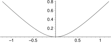
Figure 1. Case (A), $Q(z)=z^{2}(\textrm{i}-1/z)$

An example, which is simpler to compute, however not in the form (5.1), is

$$Q(z)=\frac{z^{2}}{(z-\textrm{i})(z+\textrm{i})}\,\left(\textrm{i}-\frac{1}{z}\right)=\frac{\textrm{i}z}{z-\textrm{i}}.$$

Solving

$$\frac{\textrm{i}z}{z-\textrm{i}}=\tau$$

one gets

$$\alpha(\tau)=\frac{-\tau+\tau^{2}\textrm{i}}{\tau^{2}+1},$$

and the same effect of approaching the origin tangentially from both sides is obtained.

Example 5.2.

To illustrate Case (B) consider for $\theta_{0}\in[0,\pi]$ the function

$$Q(z)=z^{2}{\rm e}^{\textrm{i}\theta_{0}}.$$

Solving $Q(z)=\tau$ with $z\in{\mathbb{C}}^{+}$ one obtains

$$\alpha(\tau)=\begin{cases}\sqrt{|\tau|}\cdot{\rm e}^{\textrm{i}(\pi-\theta_{0})/2},&\tau\leq 0,\\ \sqrt{\tau}\cdot{\rm e}^{\textrm{i}(2\pi-\theta_{0})/2},&\tau>0.\end{cases}$$

As another example of Case (B) consider

$$Q(z)=z^{2}\int_{-1}^{1}\frac{dt}{t-z}.$$

Figure 2 contains the plot of points $z\in{\mathbb{C}}^{+}$ satisfying ${\rm Im\,}Q(z)=0$.

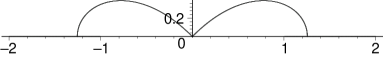
Figure 2. Case (B), $Q(z)=z^{2}\int_{-1}^{1}\frac{dt}{t-z}$.

Since $\alpha(\infty)=\infty$ one sees that for sufficiently small $\tau<0$ the point $\alpha(\tau)$ moves with increasing $\tau$ along the real line to the left until it reaches the point near $1.7$. There it leaves the real line to the upper half–plane and continues along the plotted path until it reaches the real line again at approximately $-1.7$. From that point it continues along the real line.

Example 5.3.

To illustrate Case (C) consider the function

$$Q(z)=z^{2}\left(1+\int_{-1}^{1}\frac{t^{2}\ dt}{t-z}\right).$$

Figure 3 contains the plot of points $z\in{\mathbb{C}}^{+}$ satisfying ${\rm Im\,}Q(z)=0$. One may observe that with $\tau\downarrow 0$ the point $\alpha(\tau)$ approches the real line approximately vertically and it leaves the origin approximately horizontally. It is known from Theorem 3.6 of [15] that the only point in a neighborhood of zero where $\alpha(\tau)\in{\mathbb{R}}$ is the origin itself.

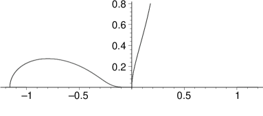
Figure 3. Case (C), $Q(z)=z^{2}\left(1+\int_{-1}^{1}\frac{t^{2}\ dt}{t-z}\right)$

Example 5.4.

To illustrate Case (D) consider the function

$$Q(z)=z^{2}\int_{-1}^{1}\frac{t^{2}}{t-z}dt.$$

Figure 4 contains the plot of points $z\in{\mathbb{C}}^{+}$ satisfying ${\rm Im\,}Q(z)=0$. Note the essential difference between Figure 2 and Figure 4, in Figure 2 the angle between the left and right limit of $\alpha(\tau)$ at the origin is $\pi/2$, while in Figure 4 it is $\pi/3$. The movement of $\alpha(\tau)$ along the plotted line and the real line is the same as in Example 5.2.

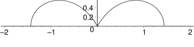
Figure 4. Case (D), $Q(z)=z^{2}\left(\int_{-1}^{1}\frac{t^{2}\ dt}{t-z}\right)$

Example 5.5.

Finally, to illustrate Case (E) consider the function

$$Q(z)=z^{2}\left(\int_{-1}^{1}\frac{t^{4}\ dt}{t-z}\right).$$

Figure 5 contains the plot of points $z\in{\mathbb{C}}^{+}$ satisfying ${\rm Im\,}Q(z)=0$. The angle between the left and right limit of $\alpha(\tau)$ at the origin is $\pi/3$ and the movement of $\alpha(\tau)$ along the plotted line and the real line is the same as in Examples 5.2 and 5.3.

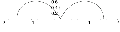
Figure 5. Case (E), $Q(z)=z^{2}\left(\int_{-1}^{1}\frac{t^{4}\ dt}{t-z}\right)$

References

- [1] M. S. Derevyagin, and V. A. Derkach, “On the convergence of Pade approximants of generalized Nevanlinna functions”, Tr. Mosk. Mat. Obs., 68 (2007), 133–182; english translation in Trans. Moscow Math. Soc. 2007, 119–162.
- [2] V. Derkach, S. Hassi, and H.S.V. de Snoo, “Operator models associated with Kac subclasses of generalized Nevanlinna functions”, Methods of Functional Analysis and Topology, 5 (1999), 65–87.
- [3] V.A. Derkach, S. Hassi, and H.S.V. de Snoo, “Rank one perturbations in a Pontryagin space with one negative square”, J. Funct. Anal., 188 (2002), 317–349.
- [4] A. Dijksma, H. Langer, A. Luger, and Yu. Shondin, “A factorization result for generalized Nevanlinna functions of the class ”, Integral Equations Operator Theory, 36 (2000), 121–125.
- [5] W.F. Donoghue, Monotone matrix functions and analytic continuation, Springer-Verlag, New York-Heidelberg, 1974.
- [6] E. Hille, Analytic function theory, Volume I, Blaisdell Publishing Company, New York, Toronto, London, 1965.
- [7] P. Jonas and H. Langer, “A model for –selfadjoint operator in a space and a special linear pencil”, Integral Equations Operator Theory, 8 (1985), 13–35.
- [8] M.G. Kreĭn and H. Langer, “Über die -function eines -hermiteschen Operators im Raume ”, Acta. Sci. Math. (Szeged), 34 (1973), 191–230.
- [9] M.G. Kreĭn and H. Langer, “Über einige Fortsetzungsprobleme, die eng mit der Theorie hermitescher operatoren im Raume zusammenhangen. I. Einige Funktionenklassen und ihre Darstellungen”, Math. Nachr., 77 (1977), 187–236.
- [10] H. Langer, “Spectral functions of definitizable operators in Krein spaces”, Proceedings Functional Analysis, Dubrovnik 1981, Lecture Notes in Math., 948, Springer Verlag, Berlin, 1982, 1–46.
- [11] H. Langer, “A characterization of generalized zeros of negative type of functions of the class ”, Oper. Theory Adv. Appl., 17 (1986), 201–212.
- [12] H. Langer, A. Luger, and V. Matsaev, “Convergence of generalized Nevanlinna functions”, Acta Sci. Math. (Szeged), 77 (2011), 425–437.
- [13] P. Pagacz, and M. Wojtylak, “Dyck paths and –selfadjoint Wigner matrices”, preprint.
- [14] E.A. Rakhmanov, “O skhodimosti diagonalnych approksimacij Pade” [On convergence of the diagonal Pade approximations] Mat. Sb., 104 (1977), 271–291.
- [15] H.S.V. de Snoo, H. Winkler, and M. Wojtylak, “Zeros and poles of nonpositive type of Nevanlinna functions with one negative square”, J. Math. Ann. Appl., 382 (2011), 399–417.
- [16] M. Wojtylak, “On a class of –selfadjoint random matrices with one eignvalue of nonpositive type”, Electron. Commun. Probab., 17 (2012), no. 45, 1–14.