Inertial longitudinal magnetization reversal for non-Heisenberg ferromagnets

Abstract

We analyze theoretically the novel pathway of ultrafast spin dynamics for ferromagnets with high enough single-ion anisotropy (non-Heisenberg ferromagnets). This longitudinal spin dynamics includes the coupled oscillations of the modulus of the magnetization together with the quadrupolar spin variables, which are expressed through quantum expectation values of operators bilinear on the spin components. Even for a simple single-element ferromagnet, such a dynamics can lead to an inertial magnetization reversal under the action of an ultrashort laser pulse.

I Introduction

Which is the fastest way to reverse the magnetization of either a magnetic particle or a small region of a magnetic film? This question has attracted significant interest, both fundamental and practical, for magnetic information storage. [1] Intense laser pulses, with durations less than a hundred femtoseconds, are able to excite the ultrafast evolution of the total spin of a magnetically-ordered system on a picosecond time scale, see e.g. the reviews. [2] ; [3] ; [4] The limitations for the time of magnetization reversal come from the characteristic features of the spin evolution for a magnet with a concrete type of magnetic order. The dynamical time cannot be shorter than the characteristic period of spin oscillations $T$, $T=2\pi/\omega_{0}$, where $\omega_{0}$ is the magnetic resonance frequency. For ferromagnets, the frequency of standard spin oscillations (precession) is $\omega_{0,\mathrm{FM}}=\gamma H_{\mathrm{r}}$, where $\gamma$ is the gyromagnetic ratio, and $H_{\mathrm{r}}$ is an effective field of relativistic origin, like the anisotropy field, which is usually less than a few Tesla. Thus, the dynamical time for Heisenberg ferromagnets cannot be much shorter than one nanosecond. For antiferromagnets, all the dynamical characteristics are exchange enhanced, and $\omega_{0,\mathrm{AFM}}=\gamma\sqrt{H_{\mathrm{ex}}H_{\mathrm{r}}}$, where $H_{\mathrm{ex}}$ is the exchange field, $H_{\mathrm{ex}}=J/2\mu_{\mathrm{B}}$, $J$ is the exchange integral, and $\mu_{\mathrm{B}}$ is the Bohr magneton, see Ref. [5], . The excitation of terahertz spin oscillations has been experimentally demonstrated for transparent antiferromagnets using the inverse Faraday effect or the inverse Cotton-Mouton effect. [6] ; [7] ; [8] ; [9] ; [10] ; [11] The non-linear regimes of such dynamics include the inertia-driven dynamical reorientation of spins on a picosecond time scale, which was observed in orthoferrites. [10] ; [11]

The exchange interaction is the strongest force in magnetism, and the exchange field $H_{\mathrm{ex}}$ can be as strong as $10^{3}$ Tesla. The modulus of the magnetization is determined by the exchange interaction, and the direction of the magnetization is governed by relativistic interactions. It would be very tempting to produce a magnetization reversal by changing the modulus of the magnetization vector, i.e., via the longitudinal dynamics of ${\rm{\bf M}}$. For such a process, dictated by the exchange interaction, the characteristic times could be of the order of the exchange time $\tau_{\mathrm{ex}}=1/\gamma H_{\mathrm{ex}}$, which is shorter than one picosecond. However, within the standard approach such dynamics is impossible. The evolution of the modulus of the magnetization, $M=|{\rm{\bf M}}|$, within the closed Landau-Lifshitz equation for the magnetization only (or the set of such equations for the sublattice magnetizations, ${\rm{\bf M}}_{\alpha})$, is purely dissipative. [12] This feature could be explained as follows: two angular variables, $\theta$ and $\varphi$, describing the direction of the vector ${\rm{\bf M}}$, within the Landau-Lifshitz equation determine the pair of conjugated Hamilton variables $(\cos\theta$ and $\varphi$ are the momentum and coordinate, respectively). Also, the evolution of the single remaining variable $M=|{\rm{\bf M}}|$, governed by a first-order equation can be only dissipative; see a more detailed discussion below. Moreover, the exchange interaction conserves the total spin of the system, and the relaxation of the total magnetic moment of any magnet can be present only when accounting for relativistic effects. Thus the relaxation time for the total magnetic moment is relativistic but it is exchange-enhanced, as was demonstrated within the irreversible thermodynamics of the magnon gas. [12] Note here that the relaxation of the magnetization of a single sublattice for multi-sublattice magnets can be of purely exchange origin. [13] Recently, magnetization reversal on a picosecond time scale has been experimentally demonstrated for the ferrimagnetic alloy GdFeCo, see Refs. [13], ; [14], . These results can be explained within the concept of exchange relaxation, developed by Baryakhtar, [15] accounting for the purely exchange evolution of the sublattice magnetization. [16] Such an exchange relaxation can be quite fast, but its characteristic time is again longer than the expected “exchange time” $\tau_{\mathrm{ex}}=1/\gamma H_{\mathrm{ex}}$.

Thus, the ultrafast mechanisms of magnetization reversal implemented so far are: the dynamical (inertial) switching possible for antiferromagnets, [10] ; [11] and the exchange longitudinal evolution for ferrimagnets. [13] ; [14] ; [16] These are both quite fast, with a characteristic time of the order of picoseconds; but their characteristic times are longer than the “ideal estimate”: the exchange time $\tau_{\mathrm{ex}}$.

In this work, we present a theoretical study of the possibility of the dynamical evolution of the modulus of the magnetization for non-Heisenberg ferromagnets with high enough single-ion anisotropy that can be called longitudinal spin dynamics. For such a dynamics, an inertial magnetization reversal is possible even for a simple single-element ferromagnet. Longitudinal dynamics does not exist in Heisenberg magnets, and this dynamics cannot be described in terms of the Landau-Lifshitz equation, or using the Heisenberg Hamiltonian, which is bilinear over the components of spin operators for different spins, see more details below in Sec. II. The key ingredient of our theory is the inclusion of higher-order spin quadrupole variables. It is known that for magnets with atomic spin $S>1/2$, allowing the presence of single-ion anisotropy, the spin dynamics is not described by a closed equation for spin dipolar variable $\left\langle{\rm{\bf S}}\right\rangle$ alone (or magnetization ${\rm{\bf M}}=-2\mu_{\mathrm{B}}\left\langle{\rm{\bf S}}\right\rangle$). [17] ; [18] ; [19] ; [20] ; [21] ; Chubuk90 ; Matveev ; AndrGrishchuk Here and below $\left\langle{...}\right\rangle$ means quantum and (at finite temperature) thermal averaging. To be specific, we choose the spin-one ferromagnet with single-ion anisotropy, the simplest system allowing this effect. The full description of these magnets requires taking into account the dynamics of quadrupolar variables, $S_{ik}=(1/2)\left\langle{S_{i}S_{k}+S_{k}S_{i}}\right\rangle$, that represent the quantum averages of the operators, bilinear in the spin components. Our theory is based on the consistent semiclassical description of a full set of spin quantum expectation values (dipolar and quadrupolar) for the spin-one system, which was investigated by many authors from different viewpoints. [17] ; [18] ; [19] ; [20] ; [21] ; Chubuk90 ; Matveev ; AndrGrishchuk As we will show, the longitudinal dynamics of spin, including nonlinear regimes, can be excited by a femtosecond laser pulse. With natural accounting for the dissipation, the longitudinal spin dynamics can lead to changing the sign of the total spin of the system (longitudinal magnetization reversal).

II MODEL DESCRIPTION

The Landau-Lifshitz equation was proposed many years ago as a phenomenological equation, and it is widely used for the description of various properties of ferromagnets. Concerning its quantum and microscopic basis, it is worth noting that this equation naturally arises using the so-called spin coherent states. [22] ; [23] These states can be introduced for any spin $S$ as the state with the maximum value of the spin projection on an arbitrary axis ${\rm{\bf n}}$. Such states can be parameterized by a unit vector ${\rm{\bf n}}$; the direction of the latter coincides with the quantum mean values for the spin operator $\left\langle{\rm{\bf S}}\right\rangle=S{\rm{\bf n}}$ (dipolar variables). This property is quite convenient for linking the quantum physics of spins to a phenomenological Landau-Lifshitz equation. The use of spin coherent states is most efficient when the Hamiltonian of the system is linear with respect to the operators of the spin components. If an initial state is described by a certain spin coherent state, its quantum evolution will reduce to a variation of the parameters of the state (namely, the direction of the unit vector ${\rm{\bf n}})$, which are described by the classical Landau-Lifshitz equation. Thus, spin coherent states are a convenient tool for the analysis of spin Hamiltonians containing only operators linear on the spin components or their products on different sites. An important example is the bilinear Heisenberg exchange interaction, described by the first term in Eq. (1) below.

In contrast to the cases above, for the full description of spin-$S$ states, one needs to introduce $SU(2S+1)$ generalized coherent states. [17] ; [19] ; [20] ; [21] The analysis shows that spin coherent states are less natural for the description of magnets whose Hamiltonian contains products of the spin component operators at a single site. Such terms are present for magnets with single-ion anisotropy or a biquadratic exchange interaction. Magnets with non-small interaction of this type are often called non-Heisenberg. For such magnets, some non-trivial features, absent for Heisenberg magnets, are known. Among them we note the possibility of so-called quantum spin reduction; namely the possibility to have the value of $|\left\langle{\rm{\bf S}}\right\rangle|$ less than its nominal value, $|\left\langle{\rm{\bf S}}\right\rangle|<S$, even for pure states at zero temperature. This was first mentioned by Moriya, [24] as early as 1960. As an extreme realization of the effect of quantum spin reduction, we note the existence of the so-called spin nematic phases with a zero mean value of the spin in the ground state at zero temperature. In the last two decades, the interest on such states has been considerable, motivated by studies of multicomponent Bose-Einstein condensates of atoms with non-zero spin. [25] ; [26] ; [27] ; [28]

A significant manifestation of quantum spin reduction is the appearance of an additional branch of the spin oscillations, which is characterized by the dynamics (oscillations) of the length of the mean value of spin without spin precession. [17] ; [18] ; [19] ; [20] ; [21] ; Chubuk90 ; Matveev The characteristic frequency of this mode can be quite high (of the order of the exchange integral). For this reason, for a description of resonance properties or thermodynamic behavior of magnets, this mode is usually neglected, and the common impression is that the dynamics of magnetic materials with constant single-ion anisotropy $K<$(0.2-0.3)$J$ is fully described by the standard phenomenological theory. However, for an ultrafast evolution of the spin system under a femtosecond laser pulse, one can expect a lively demonstration of this longitudinal high-frequency mode. Thus, it is important to explore the possible manifestations of the effects of quantum spin reduction in the dynamic properties of ferromagnets.

The simplest model allowing spin dynamics with effects of quantum spin reduction is described by the Hamiltonian

$$H=-\frac{1}{2}\sum\limits_{\mathbf{n},\boldsymbol{\ell}}{\bar{J}{\rm{\bf S}}_{\mathbf{n}}{\rm{\bf S}}_{\mathbf{n}+\boldsymbol{\ell}}}+\frac{K}{2}\sum\limits_{\mathbf{n}}{\left({S_{\mathbf{n},x}}\right)^{2}},$$ (1)

where ${\rm{\bf S}}_{\mathbf{n}}$ is the spin-one operator at the site $\mathbf{n}$; $\bar{J}>0$ is the exchange constant for nearest-neighbors $\boldsymbol{\ell}$, and $K>0$ is the constant of the easy-plane anisotropy with the plane $yz$ as the easy plane. The quantization axis can be chosen parallel to the $z$-axis and $\left\langle{\rm{\bf S}}\right\rangle=\left\langle{S_{z}}\right\rangle{\rm{\bf e}}_{z}$. For the full description of spin $S=1$ states, let us introduce $SU(3)$ coherent states [17] ; [19] ; [20] ; [21]

$$\left|{\mathbf{u},\mathbf{v}}\right\rangle=\sum\limits_{j=x,y,z}{\left({u_{j}+iv_{j}}\right)\left|{\psi_{j}}\right\rangle},$$ (2)

where the states $\left|{\psi_{j}}\right\rangle$ determine the Cartesian states for $S=1$ and are expressed in terms of the ordinary states {$\left|{\pm 1}\right\rangle,\;\left|0\right\rangle$} with given projections $\pm 1,\;0$ of the operator $S_{z}$ by means of the relations $\left|{\psi_{x}}\right\rangle=\left({\left|{-1}\right\rangle-\left|{+1}\right\rangle}\right)/\sqrt{2}$, $\left|{\psi_{y}}\right\rangle=i\left({\left|{-1}\right\rangle+\left|{+1}\right\rangle}\right)/\sqrt{2}$, $\left|{\psi_{z}}\right\rangle=\left|0\right\rangle$, with the real vectors $\mathbf{u}$ and $\mathbf{v}$ subject to the constraints $\mathbf{u}^{2}+\mathbf{v}^{2}=1$, $\mathbf{u}\cdot\mathbf{v}=0$. All irreducible spin averages, which include the dipolar variable $\left\langle\mathbf{S}\right\rangle$ (average value of the spin) and quadrupole averages $S_{ik}$, bilinear over the spin components, can be written through $\mathbf{u}$ and $\mathbf{v}$ as follows

$$\left\langle\mathbf{S}\right\rangle = 2(\mathbf{u}\times\mathbf{v}),$$

$$S_{ik}=\frac{1}{2}\left\langle{S_{i}S_{k}+S_{k}S_{i}}\right\rangle = \delta_{ik}-u_{i}u_{k}-v_{i}v_{k}.$$ (3)

At zero temperature and within the mean-field approximation, the spin dynamics is described by the Lagrangian [21]

$$L=-2\hbar\sum\limits_{n}{\mathbf{v}_{n}(\partial\mathbf{u}_{n}/\partial t})-W\left({\mathbf{u},\mathbf{v}}\right),$$ (4)

where $W\left({\mathbf{u},\mathbf{v}}\right)=\left\langle{\mathbf{u},\mathbf{v}}\right|H\left|{\mathbf{u},\mathbf{v}}\right\rangle$ is the energy of the system.

We are interested in spin oscillations which are uniform in space, and hence we assume that the discrete variables $\mathbf{u}$ and $\mathbf{v}$ have the same values for all spins and are only dependent on time. The frequency spectrum of linear excitations, which consists of two branches, can be easily obtained on the basis of the linearized version of the Lagrangian (4). In the general case, the system of independent equations for $\mathbf{u}$ and $\mathbf{v}$, taking into account the aforementioned constrains $\mathbf{u}^{2}+\mathbf{v}^{2}=1$, $\mathbf{u}\cdot\mathbf{v}=0$, consists of four nonlinear equations, describing two different regimes of spin dynamics. One regime is similar to that for an ordinary spin dynamics treated on the basis of the Landau-Lifshitz equation; it corresponds to oscillations of the spin direction. The second regime corresponds to oscillations of the modulus of the magnetization $\left\langle{\rm{\bf S}}\right\rangle=S(t){\rm{\bf e}}_{z}$, with the vectors $\mathbf{u}$ and $\mathbf{v}$ rotating in the $xy$-plane perpendicular to $\left\langle{\rm{\bf S}}\right\rangle$. This mode of the spin oscillations corresponds to the longitudinal spin dynamics. It is convenient to consider these two types of dynamics separately. Particular non-linear longitudinal solutions, with $\left\langle{\rm{\bf S}}\right\rangle=s(t){\rm{\bf e}}_{z}$ and $u_{z}=0,\;v_{z}=0$, were found in Refs. [29], ; [30], . Note here that the longitudinal dynamics is much faster than the standard transversal one, and the standard spin precession (described by the Landau-Lifshitz equation) at a picosecond time scale just cannot develop. Therefore, these two regimes, longitudinal and transverse, can be treated independently, and we limit ourselves only to the longitudinal dynamics with $\left\langle{\rm{\bf S}}\right\rangle=s(t){\rm{\bf e}}_{z}$ and $u_{z}=0,\;v_{z}=0$.

III LONGITUDINAL SPIN DYNAMICS

To describe the longitudinal spin dynamics, it is convenient to introduce new variables: the spin modulus $s=2|{\rm{\bf u}}||{\rm{\bf v}}|=2uv$ and angular variable $\gamma$, with

$${\rm{\bf u}}=u\left({{\rm{\bf e}}_{x}\cos\gamma-{\rm{\bf e}}_{y}\sin\gamma}\right),\;{\rm{\bf v}}=v\left({{\rm{\bf e}}_{x}\sin\gamma+{\rm{\bf e}}_{y}\cos\gamma}\right),$$ (5)

In this representation $\left\langle{S_{z}}\right\rangle=s$, and the non-trivial quadrupolar variables are $\left\langle{S_{x}S_{y}+S_{y}S_{x}}\right\rangle=\sqrt{1-s^{2}}\sin 2\gamma$ and $\left\langle{S_{y}^{2}-S_{x}^{2}}\right\rangle=\sqrt{1-s^{2}}\cos 2\gamma$, with all other quantum averages being either zero (as the transverse spin components $\left\langle{S_{x,y}}\right\rangle$ or $S_{xz}$, $S_{yz}$) or trivial, independent on $s$ and $\gamma$, as $\left\langle{S_{z}^{2}}\right\rangle=1$. The mean-field energy, written per one spin through the variables $s,\;\gamma$, takes the form

$$W(s,\gamma)=-\frac{J}{2}s^{2}-\frac{K}{4}\sqrt{1-s^{2}}\cos 2\gamma,$$ (6)

where $J=\bar{J}Z$, $Z$ is the number of nearest neighbors. The ground state at $\sqrt{1-s^{2}}>0$ corresponds to $\cos 2\gamma=1$, with the mean value of the spin $s=\pm\bar{s}$, $\bar{s}=\sqrt{1-\kappa^{2}}<1$, that is a manifestation of quantum spin reduction at non-zero anisotropy. Here we introduce the dimensionless parameter $\kappa=K/4J$. For these variables, the Lagrangian can be written as

$$L=\hbar s\frac{\partial\gamma}{\partial t}-W(s,\gamma),$$ (7)

and $\hbar s$ and $\gamma$ play the role of canonical momentum and coordinate, respectively, with the Hamilton function $W(s,\gamma)$. The physical meaning of the above formal definitions is quite clear: the angular variable $\gamma$ describes the transformation of quadrupolar variables under rotation around the $z$-axis, with $\hbar s$ as the projection of the angular momentum on this axis.

III.1 Small oscillations

Let us now start with the description of the dynamics of small-amplitude oscillations. After linearization around the ground state, the equation leads to a simple formula for the frequency of longitudinal oscillations

$$\hbar\omega_{l}=2J\bar{s}=2J\sqrt{1-\kappa^{2}},$$ (8)

which are in fact coupled oscillations of the projection of the spin and quadrupolar variables, see Fig. 1.

One can see that, for a wide range of values of the anisotropy constant, like $\kappa<0.2$-0.8, this frequency $\omega_{l}$ is of the order of (1.8-1.2)$J/\hbar$, i.e., $\omega_{l}$ is comparable to the exchange frequency $J/\hbar$. Thus the longitudinal spin dynamics is expected to be quite fast. In contrast, standard transversal oscillations for a purely easy-plane model (1) are gapless (they acquire a finite gap when accounting for a magnetic anisotropy in the easy plane, which is usually small). Thus the essential difference in the frequencies of these two dynamical regimes is clearly seen.

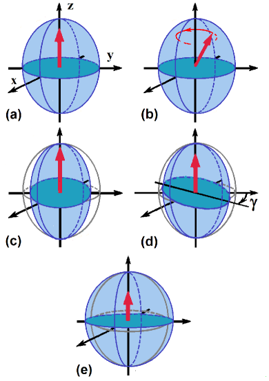
Figure 1: (color online) Graphic presentation of the variables $s$ and $\gamma$ and their evolution. The thick red arrow represents the mean value of the spin. The quadrupolar variables are shown by the blue three-axial ellipsoid with the directions of the main axis (chosen to have $\left\langle{S_{1}S_{2}}\right\rangle=0)$: ${\rm{\bf e}}_{3}={\rm{\bf e}}_{z}$ and ${\rm{\bf e}}_{1}$, ${\rm{\bf e}}_{2}$. The half-axes of the ellipsoid are equal to $\left\langle{S_{1}^{2}}\right\rangle$, $\left\langle{S_{2}^{2}}\right\rangle$ and $\left\langle{S_{3}^{2}}\right\rangle=\left\langle{S_{z}^{2}}\right\rangle=1$. (a) the ground state, (b) the standard transverse dynamics, i.e. the spin precession. The other frames (c)-(e) present the transient values of the variables in longitudinal oscillations. (c) and (e) correspond to the longest and shortest length of the spin, and at the moment depicted in (d) the spin length equals to its equilibrium value, but the quadrupolar ellipsoid is turned on the angle $\gamma$ with respect to the $x$-axis. On the frames (c)-(e), the shape of the unperturbed ellipsoid is shown by light grey.

At a first glance, there is a contradiction between the concept of longitudinal dynamics caused by single-ion anisotropy and the result present in equation (8): the value of $\omega_{l}$ is still finite for vanishing anisotropy constant $K$; and it is even growing to the value $2J/\hbar$ when $\kappa\to 0$. This can be explained as follows: for a given energy, the ratio of amplitudes for the oscillations of the spin variable $s$ and quadrupolar variable $\gamma$ vanish at $\kappa\to 0$ as $\kappa$. In fact, for extremely low anisotropy the spin oscillations are not present in this mode, which becomes just a free rotation of the quadrupole ellipsoid of the form $\gamma=2Jt/\hbar$, with $s=\bar{s}=\mathrm{const}$. On a phase plane with coordinates $(s,\gamma)$ this dynamics is depicted by vertical straight lines parallel to the $\gamma$-axis, see Fig. 2(c) below. We will discuss this feature in more detail with the analysis of non-linear oscillations.

III.2 Nonlinear dynamics and phase plane analysis.

Before considering damped oscillations, it is instructive to discuss dissipationless non-linear longitudinal oscillations. It is convenient to present an image of the dynamics as a “phase portrait” on the plane momentum-coordinate $(s,\;\gamma)$, which shows the behavior of the system for arbitrary initial conditions. The phase trajectories in the plane without dissipation can be found from the condition $W(s,\gamma)=\mathrm{const}$.

The energy (6) has an infinite set of minima, with $s=\pm\bar{s}$ and $\gamma=\pi n,$ with equal energies (green ellipses on the Fig.2), and an infinite set of maxima at $s=0$ and $\gamma=\pi/2+\pi n$ (red ellipses on the Fig.2), here $n$ is an integer. Only the minima with $s=\bar{s}$ and $s=-\bar{s}$ are physically different; equivalent extremes with different values of $n$ correspond to the equal values of the observables and are completely equivalent. The minima on the phase plane correspond to foci with two physically different equilibrium states with antiparallel orientation of spin $s=\pm\bar{s}$, and $\left\langle{S_{y}^{2}-S_{x}^{2}}\right\rangle=\sqrt{1-\bar{s}^{2}}$, $\left\langle S_{z}^{2}\right\rangle=1$, $\left\langle{S_{x}S_{y}+S_{y}S_{x}}\right\rangle=0$. The saddle points are located at the values $s=0$ and $\gamma=\pi n$. The lines with $s=\pm 1$ are singular; these correspond to degenerate motion with $\gamma$ linear in time $\gamma=\pm tJ/\hbar$; the points at these lines where $d\gamma/dt$ change sign, can be treated as some non-standard saddle points.

The shape of the phase trajectories, i.e., the characteristic features of oscillations, varies with the change of the anisotropy parameter $\kappa$. Note first the general trend, the relative amplitude of the changes of the spin and $\gamma$ depends on $\kappa$: the bigger $\kappa$ is, the larger values of the change of spin are observed. The topology of the phase trajectories change at the critical value of the anisotropy parameter $\kappa$. At small $\kappa<1/2$, the trajectories with infinite growing $\gamma$ are present, and the standard separatrix trajectories connect together different saddle points, see Fig. 2 (c). As mentioned above; only such trajectories are present at the limit $\kappa\to 0$, but, in fact, even for the small value of $\kappa=0.2$ used in Fig.2 (c), the main part of the plane is occupied by the trajectories that change the spin. At the critical value $\kappa=1/2,$ the separatrix trajectories connect the saddle points at $s=0$, $\gamma=0$ and the degenerated saddle points at the singular lines with $s=\pm 1$. At larger anisotropy $\kappa>1/2$, as in Fig. 2(a), the only separatrix loops entering the same saddle point are present.

The minima, saddle point and the separatrix are the key ingredients for the switching between the ground states with $s=\bar{s}$ and $s=-\bar{s}$. The case of large anisotropy $\kappa>1/2$ looks like the standard one for the switching phenomena, whereas for small anisotropy the situation is more complicated.

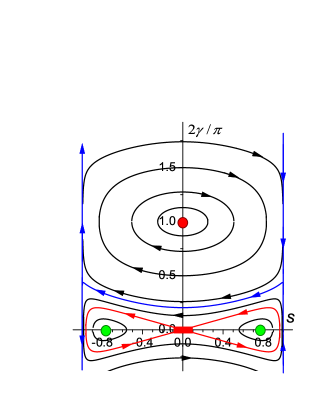
(a) $\ \kappa=$0.6

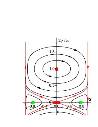
(b) $\ \kappa=$0.5

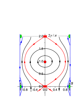
(c) $\ \kappa=$0.2

Figure 2: (color online) Phase plane representations for dissipation-free non-linear longitudinal spin oscillations for different values of the parameter $\kappa$; $\kappa=$0.6, 0.5 and 0.2 for panels (a), (b), and (c), respectively. The green and red ellipses present the minima and maxima, respectively; the standard saddle points are depicted by red rectangles, while the standard separatrix trajectories are drawn by red lines. The singular trajectories with $s=\pm 1$ and the separatrix trajectories entering the non-standard saddle points on these lines $s=\pm 1$ are shown by blue lines on the frames (a) and (c). For the critical value $\kappa=0.5$, all the separatrix trajectories and the singular trajectories with $s=\pm 1$ organize a common net; and on the corresponding frame (b) all of them are presented by red lines.

III.3 Damped longitudinal motion

Damping is a crucial ingredient for the dynamical switching between different, but equivalent in energy, states. The high-frequency mode of longitudinal oscillations have high-enough relative damping; as was found from microscopic calculations, [29] the decrement of longitudinal mode $\Gamma=\lambda\omega_{l}$, where $\lambda\sim 0.2$. To account for the damping in the dynamic equations for $s$ and $\gamma$, it is useful to consider a different parametrization of the longitudinal dynamics. Let us now introduce a unit vector, $\boldsymbol{\sigma}=\sigma_{1}{\rm{\bf e}}_{1}+\sigma_{2}{\rm{\bf e}}_{2}+\sigma_{3}{\rm{\bf e}}_{3}$, with components $\sigma_{3}=s$, $\sigma_{1}=\langle S_{y}^{2}-S_{x}^{2}\rangle,$ and $\sigma_{2}=\langle S_{1}S_{2}+S_{2}S_{1}\rangle$. Being written through $\boldsymbol{\sigma}$, the equation of motion takes the form of the familiar Landau-Lifshitz equation

$$\hbar\frac{\partial\boldsymbol{\sigma}}{\partial t}=[\boldsymbol{\sigma}\times{\rm{\bf h}}_{\mathrm{eff}}]+{\rm{\bf R}},\quad{\rm{\bf h}}_{\mathrm{eff}}=-\frac{\partial W}{\partial\boldsymbol{\sigma}},$$ (9)

where ${\rm{\bf h}}_{\mathrm{eff}}$ can be treated as an effective field for longitudinal dynamics, and the relaxation term ${\rm{\bf R}}$ is added. The equation of motion with ${\rm{\bf R}}=0$ is fully equivalent to the Hamilton form of the equation found from (7), but the form of the dissipation is more straightforward in unit-vector presentation. The choice of the damping term in a standard equation for the motion of the transverse spin is still under debate, see. [15] ; [31] But here the damping term can be written in the simplest form, as in the original paper of Landau and Lifshitz, ${\rm{\bf R}}=\lambda[{\rm{\bf h}}_{\mathrm{eff}}-\boldsymbol{\sigma}({\rm{\bf h}}_{\mathrm{eff}}\boldsymbol{\sigma})]$. The arguments are as follows: (i) this form gives the correct value of the decrement of linear oscillations, $\Gamma=\lambda\omega_{l}$; (ii) it is convenient for analysis, because it keeps the condition $\boldsymbol{\sigma}^{2}=1$. Finally, the equations of motion with the dissipation term of the aforementioned form are:

$$\hbar\frac{ds}{dt}=-\frac{\partial W}{\partial\gamma}-\lambda(1-s^{2})\frac{\partial W}{\partial s},\;\hbar\frac{d\gamma}{dt}=\frac{\partial W}{\partial s}-\frac{\lambda}{(1-s^{2})}\frac{\partial W}{\partial\gamma}.$$ (10)

These equations describe the damped counterpart of the non-linear longitudinal oscillations discussed in the previous subsection and present as phase portraits on Fig. 2. The character of the motion at not-too-large $\lambda$ can be qualitatively understood from energy arguments. The trajectories of damped oscillations in any point of the phase plane approximately follow the non-damped (described by equation $W(s,\gamma)=\mathrm{const})$ ones, but cross them passing from larger to smaller values of $W$, see Figs. 3 and 4. It happens that for the case of interest, the dynamics is caused by the time-dependent stimulus. An action of the stimulus on the system can be described by adding the corresponding time-dependent interaction energy $\Delta W$ to the system Hamiltonian, $W\to W(s,\gamma)+\Delta W(s,\gamma,t)$. Within this dynamical picture, $\Delta W$ produces an “external force” driving the system far from equilibrium.

The analysis is essentially simplified for a pulse-like stimulus of a short duration $\Delta t$ (much shorter than the period of motion, $\omega_{l}\Delta t\ll 1)$. In this case, the role of the pulse is reduced to the creation of some non-equilibrium state, which then evolves as some damped nonlinear oscillations described by the “free” equations (10) with $\Delta W=0$. The phase plane method, which shows the behavior of the system for arbitrary initial conditions, is the best tool for the description of such an evolution.

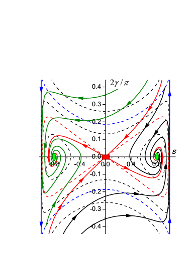
Figure 3: (color online) Phase plane representation of damped longitudinal spin oscillations for $\kappa=$0.6. Here and in Fig. 4, the dashed lines (obtained analytically before) represent the phase trajectories without dissipation, while the full lines are trajectories for dissipation constant $\lambda=0.2$, found numerically. The separatrix lines are drawn by red curves.

It is worth noting that the asymptotic behavior of the separatrix trajectories at $\gamma,s\to 0$, is important for this analysis, and can be easily found analytically as

$$\left({\frac{\gamma}{s}}\right)_{\mathrm{separ}}=R_{\mathrm{separ}}=\\ =\frac{1}{8\kappa}\left[{\lambda(1+3\kappa)+\sqrt{\lambda^{2}(1+3\kappa)^{2}+16\kappa(1-\kappa)}}\right]\quad.$$ (11)

First let us start with the analysis for high-enough anisotropy. The corresponding phase portrait is present in Fig. 3. The general property of the phase plane is that the phase trajectories cannot cross each other; they can only merge at the saddle points. Thus the trajectories coming to different minima are stretched between two separatrix lines entering the same saddle point from different directions, as shown in Fig. 3. From this it follows that any initial state with arbitrary non-equilibrium values of spin $s(+0)$, but without deviation of $\gamma$ from its equilibrium value, evolve to the state with the same sign of the spin as for $s(+0)$, and no switching occurs. On the other hand, if the initial condition is above the separatrix trajectory, entering the saddle point, the evolution will move the system to the equivalent minimum with the sign of the spin opposite to the initial one, $s(+0)$, realizing the switching.

Figure 4 shows the phase plane for equations (10) for the more complicated case of low anisotropy, demonstrating possible scenarios of the switching of the sign of the spin value during such dynamics. Here the separatrix trajectories for the damped motion can be monitored from their maxima, and the full picture of the behavior can be understood only when including a few equivalent foci with $\gamma=0,\,\pm\pi,\,\pm 2\pi$, ect., with different, but equivalent in energy, values of the spin, $s=\pm\bar{s}$, $\bar{s}=\sqrt{1-\kappa^{2}}$, and different saddle points, located at $\gamma=0,\,\pm\pi,\,\pm 2\pi$. As for small anisotropy, the trajectories coming to different minima are located between two branches of the separatrix lines, but now this “separatrix corridor” is organized by separatrix lines entering different saddle points. The switching phenomena is also possible, but the process involves a few full turns of the variable $\gamma$.

The general regulation for any anisotropy can be formulated as follows: for realizing spin switching, one needs to have the initial deviation (reduction) of the spin value, and, simultaneously, a non-zero deviation of the quadrupolar variable $\gamma$. To switch the positive spin value to negative, one needs to start from the states just above the separatrix line entering the saddle point from positive values of $s$. The smaller the initial value of the spin, the smaller value of $\gamma(0)$ would realize the switching. From the asymptotic equation (11), the corresponding ratio $R_{\mathrm{separ}}=\gamma(0)/m(0)$ is smaller for small values of $\lambda$; but even when $\lambda\to 0,$ it exceeds the value $R_{\mathrm{separ}}(\lambda=0)=0.5\sqrt{(1-\kappa)/\kappa}$. Thus, the switching could occur for non-zero values of $\kappa$.

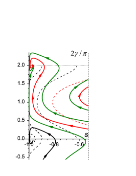
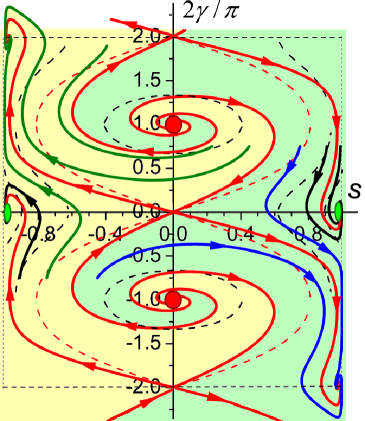
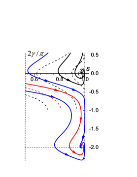
Figure 4: (color online) Phase plane for the damped spin evolutions for low anisotropy, $\kappa=0.2$. The central frame shows the full diagram; left and right panels demonstrate the details of the behavior near the equilibrium values $s=-\bar{s}$ and $s=\bar{s}$, respectively. On this frame, the regions colored by green and yellow correspond to different basins of attraction with initial values leading to the equilibrium states with $s=\bar{s}$ and $s=-\bar{s}$, respectively.

IV INTERACTION OF THE LIGHT PULSE ON THE SPIN SYSTEM: CREATION OF THE INITIAL STATE FOR SWITCHING.

Let us now consider the longitudinal spin evolution caused by a specific stimulus: a femtosecond laser pulse. The reduction of the spin to small values was observed in many experiments, and the only non-trivial remaining question is: how can we create a deviation of the quadrupolar variable $\gamma$ from its equilibrium value $\gamma=0$. To find this, we now consider possible mechanisms of light interaction with quadrupolar variables of non-Heisenberg magnets.

The interaction of the spin system of magnetically-ordered media and light is described by the Hamiltonian (as above, written per spin) $\Delta W=\bar{\varepsilon}_{ij}v_{0}E_{i}(t)E_{j}^{\ast}(t)/16\pi$, where $v_{0}$ is the volume per spin, $E_{i}(t)$ is the time-dependent amplitude of the light in the pulse, $\bar{\varepsilon}_{ij}=d(\omega\varepsilon_{ij}^{(\mathrm{spin})})/d\omega$, $\varepsilon_{ij}^{(\mathrm{spin})}$ is the spin-dependent part of the dielectric permittivity tensor, and $\omega$ is the frequency of light. For the longitudinal dynamics considered here, circularly-polarized light propagating along the $z$-axis acts on the $z$-component of the spin via the standard inverse Faraday effect, with the antisymmetric part of $\bar{\varepsilon}_{ij}^{(a)}$ as, $\bar{\varepsilon}_{xy}^{(a)}=-\bar{\varepsilon}_{xy}^{(a)}=s\alpha_{\mathrm{F}}$, giving an interaction of the form

$$\Delta W_{\mathrm{circular}}=s\frac{\alpha_{\mathrm{F}}v_{0}}{16\pi}|E_{\mathrm{circ}}|^{2}\sigma,$$ (12)

where $E_{\mathrm{circ}}$ is the (complex) amplitude, $\sigma$ describes the pulse helicity: $\sigma=\pm 1$ for right-handed and left-handed circularly polarized laser pulses. To describe qualitatively the result of the action of the light pulse, let us now assume that the pulse duration $\tau_{\mathrm{pulse}}$ is the shortest time of the problem. If the pulse duration is shorter than the period of spin oscillations, the real pulse shape can be replaced by the Dirac delta function, $|E_{\mathrm{circ}}|^{2}\to E_{\mathrm{p}}^{2}\tau_{\mathrm{pulse}}\delta(t),$ where $E_{\mathrm{p}}^{2}=\int{|E_{\mathrm{circ}}|^{2}dt}/\tau_{\mathrm{pulse}}$ characterizes the pulse intensity. (Note that this approximation is still qualitatively valid even for any comparable values of $\tau_{\mathrm{pulse}}$ and $2\pi/\omega)$ Then, using equations (10) one can find the effect produced by the pulse. Within this approximation, the action of a pulse leads to an instantaneous deviation of the variable $\gamma$ from its equilibrium value, which then evolves following the non-perturbed equations of motion (10). Keeping in mind that before the pulse action the system is in equilibrium, $s(-0)=\bar{s}$ and $\gamma(-0)=0$, it is straightforward to find the values of these variables $(s$ and $\gamma)$ after the action of the pulse, $s(+0)$ and $\gamma(+0)$. For our purposes, the non-equilibrium value of the quadrupolar variable $\gamma$ is important:

$$\gamma(+0)=-\frac{\alpha_{\mathrm{F}}}{16\pi\hbar}E_{\mathrm{p}}^{2}v_{0}\tau_{\mathrm{pulse}}\sigma.$$ (13)

The cumulative action of the circularly-polarized pulse, including an essential reduction of the spin value (caused either by thermal or non-thermal mechanisms) and the deviation of $\gamma$ described by (13) could lead to the evolution we are interested here, switching the spin of the system. Note here that for standard spin reduction the polarization of the light pulse is not essential, [32] ; [33] ; [34] whereas the values of $\gamma(+0)$ are opposite for right- and left-handed circularly polarized pulses. These features are characteristic of the effect described here. Note the recent experiment where the role of circular polarization in spin switching for GdFeCo alloy was mentioned, but the authors have attributed it to magnetic circular dichroism. [35]

V CONCLUDING REMARKS.

Let us now compare the approach developed in this article with previous results on subpicosecond spin evolution. The first experimental observation of demagnetization for ferromagnetic metals under femtosecond laser pulses shows that the magnetic moment can be quenched very fast to small values, much faster than one picosecond. [32] ; [33] ; [34] These effects are associated with a new domain of the physics of magnets, femtomagnetism, [36] and its analysis is based on the microscopic consideration of spins of atomic electrons, [37] ; [38] or itinerant electrons. [39] Not discussing this fairly promising and fruitful domain of magnetism, note that, to the best of our knowledge, no effects of magnetization reversal during this “femtomagnetic stage” has been reported in the literature. For example, the subpicosecond quenching processes for the ferromagnetic alloy GdFeCo are responsible for the creation of a far-from-equilibrium state, but the evolution of this state, giving the spin reversal, can be described within the standard set of equations for the sublattice magnetizations. [16]

In contrast, here we propose some pathway to switch the sign of the magnetic moment during extremely short times, of order of the exchange time. It is shown here that the spin dynamics for magnets with non-small single-ion anisotropy can lead to the switching of the sign of the magnetic moment via the longitudinal evolution of the spin modulus together with quadrupolar variables, i.e., quantum expectation values of operators bilinear over the spin components $S_{x}$ and $S_{y}$. It is worth to stress here that the “restoring force” for this dynamics is the exchange interaction, and the characteristic time is the exchange time. On the other hand, to realize this scenario, one needs to a have non-Heisenberg interaction, e.g., single-ion anisotropy, which couples the spin dipole and quadrupole variables.

Obviously, this effect is beyond the standard picture of spin dynamics based on any closed set of equations for the spin dipolar variables (i.e., the quantum expectation values linear on the spin components) alone. Note that our approach based on the full set of variables for the atomic spin is “more macroscopic” than the “femtomagnetic” approach, [37] ; [38] ; [39] dealing with electronic states. To realize this type of switching, it is necessary to have a significant coupling between dipolar and quadrupolar spin variables, which is present in magnets with strong single-ion anisotropy. Such anisotropy is known for the numerous magnets based on anisotropic ions of transition elements such as Ni²⁺, Cr²⁺, Fe²⁺. As the classic example, note nickel fluosilicate hexahydrate NiSiF${}_{6}\cdot$6H₂O, with spin-one Ni²⁺ ions, coupled by isotropic ferromagnetic exchange interaction and subject to high single-ion anisotropy. For this compound, the strong effect of quantum spin reduction is known, with its strength dependent on the pressure: the value of $K/J$ is growing with the pressure $P$ resulting in the value $\langle S\rangle=0.6$ at $P=6$ kbar and leading to the transition to the non-magnetic state with $\langle S\rangle=0$ at $P\sim 10$ kbar. Bar+NiSiF ; Dyakonov+jetp

A number of recent experiments were done with rare-earth transition-metals compounds. [13] ; [14] ; [35] ; [40] Note here a rich variety of non-linear spin dynamics observed for thin films of the FeTb alloy under the action of femtosecond laser pulses. [40] However, the theory developed here for simple one-sublattice ferromagnet cannot be directly applied for the description of such compounds. Ferromagnetic order with high easy-plane anisotropy is present for many heavy rare-earth elements, such as Tb and Dy at low temperatures. REbook This feature is known both for bulk monocrystals, REbook and in thin layers and superlattices, see Ref. Dy_Ysuperlattices and references wherein. Strictly speaking, in our article only spin-one ions were considered. Rare-earth metals have non-zero values of both spin and orbital momentum, forming the total angular momentum of the ion, and for their description the theory needs some modifications. However, we believe that the effects of spin switching caused by quadrupolar spin dynamics will be present as well for such magnets with high values of atomic angular momentum.

The scenario proposed here includes inertial features, with the evolution of an initial deviation from one equilibrium state to the other, located far from the initial one. The initial deviations should include both deviation of the magnetization and of the quadrupolar variable, $\gamma$. Thus the effect is based on standard magnetization reduction, but it is helicity dependent as well. The necessary initial deviations can be created by a light pulse of circular polarization and the possibility of switching depends on the connection of the initial spin direction and the pulse helicity. The possible materials should satisfy a number of general conditions: they should be very susceptible to magnetization quenching, which is typical for many materials, as well as a sizeable Faraday effect, and they should also have spin one and a high enough easy-plane anisotropy.

This work is partly supported by the Presidium of the National Academy of Sciences of Ukraine via projects no.VTs/157 (EGG) and No.0113U001823 (BAI) and by the grants from State Foundation of Fundamental Research of Ukraine No. F33.2/002 (VIB and YuAF) and No. F53.2/045 (BAI). FN acknowledges partial support from the ARO, RIKEN iTHES Project, MURI Center for Dynamic Magneto-Optics, JSPS-RFBR Contract No. 12-02-92100, Grant-in-Aid for Scientific Research (S), MEXT Kakenhi on Quantum Cybernetics, and Funding Program for Innovative R&D on S&T (FIRST).

References

- (1) J. Stöhr, and H. C. Siegmann, Magnetism: From Fundamentals to Nanoscale Dynamics (Springer, Berlin, 2006).
- (2) A. Kirilyuk, A. V. Kimel, Th. Rasing, Rev. Mod. Phys., 82, 2731 (2010).
- (3) J.-Y. Bigot and M. Vomir, Annals of Physics (Berlin) 525, No. 2-3, 2 (2013).
- (4) A. Kirilyuk, A. V. Kimel, Th. Rasing, Reports on Progress in Physics 76, 026501 (2013).
- (5) V. G. Baryakhtar, B. A. Ivanov, and M. V. Chetkin, Usp. Fiz. Nauk 146, 417 (1985); V. G. Baryakhtar, B. A. Ivanov, M. V. Chetkin, and S. N. Gadetskii, Dynamics of Topological Magnetic Solitons: Experiment and Theory (Springer-Verlag, Berlin, 1994).
- (6) A. V. Kimel, A. Kirilyuk, P. A. Usachev, R. V. Pisarev, A. M. Balbashov, and Th. Rasing, Nature (London) 435, 655 (2005).
- (7) A. M. Kalashnikova, A. V. Kimel, R. V. Pisarev, V. N. Gridnev, P. A. Usachev, A. Kirilyuk, and Th. Rasing, Phys. Rev. B 78, 104301 (2008).
- (8) T. Satoh, S.-J. Cho, R. Iida, T. Shimura, K. Kuroda, H. Ueda, Y. Ueda, B. A. Ivanov, F. Nori, and M. Fiebig, Phys. Rev. Lett. 105, 077402 (2010).
- (9) R. Iida, T. Satoh, T. Shimura, K. Kuroda, B. A. Ivanov, Y. Tokunaga, and Y. Tokura, Phys. Rev. B 84, 064402 (2011).
- (10) A. V. Kimel, B. A. Ivanov, R. V. Pisarev, P. A. Usachev, A. Kirilyuk, and Th. Rasing, Nature Phys. 5, 727 (2009).
- (11) J. A. de Jong, I. Razdolski, A. M. Kalashnikova, R. V. Pisarev, A. M. Balbashov, A. Kirilyuk, Th. Rasing, and A. V. Kimel, Phys. Rev. Lett. 108, 157601 (2012).
- (12) A. I. Akhiezer, V. G. Baryakhtar, and S. V. Peletminskii, Spin Waves (Nauka, Moscow, 1967; North-Holland, Amsterdam, The Netherlands, 1968).
- (13) I. Radu, K. Vahaplar, C. Stamm, T. Kachel, N. Pontius, H. A. Dürr, T. A. Ostler, J. Barker, R. F. L. Evans, R. W. Chantrell, A. Tsukamoto, A. Itoh, A. Kirilyuk, Th. Rasing and A. V. Kimel, Nature 472, 205 (2011).
- (14) T. A. Ostler, J. Barker, R. F. L. Evans, R. Chantrell, U. Atxitia, O. Chubykalo-Fesenko, S. ElMoussaoui, L. Le Guyader, E. Mengotti, L. J. Heyderman, F. Nolting, A. Tsukamoto, A. Itoh, D. V. Afanasiev, B. A. Ivanov, A. M. Kalashnikova, K. Vahaplar, J. Mentink, A. Kirilyuk, Th. Rasing and A. V. Kimel, Nature Communications 3, 666, (2012).
- (15) V. G. Baryakhtar, Zh. Eksp. Teor. Fiz. 87, 1501 (1984); 94, 196 (1988); Fiz. Nizk. Temp. 11, 1198 (1985).
- (16) J. H. Mentink, J. Hellsvik, D. V. Afanasiev, B. A. Ivanov, A. Kirilyuk, A. V. Kimel, O. Eriksson, M. I. Katsnelson, and Th. Rasing, Phys. Rev. Lett. 108, 057202 (2012).
- (17) V. M. Matveev, Zh. Eksp. Teor. Fiz. 65, 1626 (1973).
- (18) A. F. Andreev, I. A. Grishchuk, Zh. Eksp. Teor. Fiz. 87, 467 (1984).
- (19) N. Papanicolaou, Nucl. Phys. B 305, 367 (1988).
- (20) A. V. Chubukov, J. Phys.: Condens. Matter 2, 1593 (1990); Phys. Rev. B 43, 3337 (1991).
- (21) V. S. Ostrovskii, Zh. Eksp. Teor. Fiz. 91, 1690 (1986).
- (22) V. M. Loktev and V. S. Ostrovskii, Low Temp. Phys. 20, 775 (1994).
- (23) N. A. Mikushina and A. S. Moskvin, Phys. Lett. A 302, 8 (2002).
- (24) B. A. Ivanov and A. K. Kolezhuk, Phys. Rev. B 68, 052401 (2003).
- (25) A. M. Perelomov, Usp. Fiz. Nauk 123, 23 (1977); Generalized Coherent States and Their Applications (Springer-Verlag, Berlin, 1986).
- (26) E. Fradkin, Field Theories of Condensed Matter Systems, Frontiers in Physics, Vol. 82 (Addison-Wesley, Reading, MA, 1991).
- (27) T. Moria, Phys. Rev. 117, 635 (1960).
- (28) F. Zhou, Phys. Rev. Lett. 87, 080401 (2001); E. Demler and F. Zhou, Phys. Rev. Lett. 88, 163001 (2002); A. Imambekov, M. Lukin, and E. Demler, Phys. Rev. A 68, 063602 (2003); M. Snoek and F. Zhou, Phys. Rev. B 69, 094410 (2004).
- (29) J. Stenger, D. M. Stamper-Kurn, H. J. Miesner, A. P. Chikkatur, and W. Ketterle, Nature (London) 396, 345 (1998).
- (30) F. Zhou, Int. J. Mod. Phys. B 17, 2643 (2003).
- (31) Yu. A. Fridman, O. A. Kosmachev, A. K. Kolezhuk, and B. A. Ivanov, Phys. Rev. Lett. 106, 097202 (2011).
- (32) B. A. Ivanov, N. A. Kichizhiev, and Yu. N. Mitsai, Zh. Eksp. Teor. Fiz. 102, 618 (1992).
- (33) B. A. Ivanov, A. Yu. Galkin, R. S. Khymyn, and A. Yu. Merkulov, Phys. Rev. B 77, 064402 (2008).
- (34) V. G. Baryakhtar, B. A. Ivanov, T. K. Soboleva, and A. L. Sukstanskii, Zh. Eksp. Teor. Fiz. 91, 1454 (1986); D. A. Garanin, Phys. Rev. B 55, 3050 (1997); V. G. Baryakhtar, B. A. Ivanov, A. L. Sukstanskii, and T. K. Soboleva, Phys. Rev. B 56, 619 (1997).
- (35) E. Beaurepaire, J.-C. Merle, A. Daunois, and J.-Y. Bigot, Phys. Rev. Lett. 76, 4250 (1996).
- (36) J. Hohlfeld, E. Matthias, R. Knorren, and K. H. Bennemann, Phys. Rev. Lett. 78, 4861 (1997).
- (37) A. Scholl, L. Baumgarten, R. Jacquemin, and W. Eberhardt, Phys. Rev. Lett. 79, 5146 (1997).
- (38) A. R. Khorsand, M. Savoini, A. Kirilyuk, A. V. Kimel, A. Tsukamoto, A. Itoh, and Th. Rasing, Phys. Rev. Lett. 108, 127205 (2012).
- (39) G. Zhang, W. Hubner, E. Beaurepaire, and J.-Y. Bigot, Laser-induced ultrafast demagnetization: femtomagnetism, a new frontier? In Spin dynamics in confined magnetic structures I (eds B. Hillebrands and K. Ounadjela). Topics in Applied Physics 83, 245–288. (Springer, Berlin, 2002).
- (40) J.-Y. Bigot, M. Vomir, and E. Beaurepaire, Nature Phys. 5, 515 (2009).
- (41) G. Lefkidis, G. P. Zhang, and W. Hubner, Phys. Rev. Lett. 103, 217401 (2009).
- (42) M. Battiato, K. Carva, and P. M. Oppeneer, Phys. Rev. Lett. 105, 027203 (2010); Phys. Rev. B 86, 024404 (2012).
- (43) V. G. Bar’yakhtar, I. M. Vitebskii, A. A. Galkin, V. P. D’yakonov, I. M. Fita, and G. A. Tsintsadze, Zh. Eksp. Teor. Fiz. 84, 1083 (1983).
- (44) V. P. Dyakonov, E. E. Zubov, F. P. Onufrieva, A. V. Saiko, I. M. Fita, Zh. Eksp. Teor. Fiz. 93, 1775 (1987).
- (45) A. R. Khorsand, M. Savoini, A. Kirilyuk, A. V. Kimel, A. Tsukamoto, A. Itoh, and Th. Rasing, Phys. Rev. Lett. 110, 107205 (2013).
- (46) J. Jensen and A. R. Mackintosh, Rare Earth Magnetism: Structures and Excitations (Clarendon Press, Oxford, 1991).
- (47) A. T. D. Grünwald, A. R. Wildes, W. Schmidt, E. V. Tartakovskaya, J. Kwo, C. Majkrzak, R. C. C. Ward, and A. Schreyer, Phys. Rev. B 82, 014426 (2010).