Global simulations of magnetorotational turbulence I: convergence and the quasi-steady state

Abstract

Magnetorotational turbulence provides a viable mechanism for angular momentum transport in accretion disks. We present global, three dimensional (3D), magnetohydrodynamic accretion disk simulations that investigate the dependence of the turbulent stresses on resolution. Convergence in the time-and-volume-averaged stress-to-gas-pressure ratio, $\overline{\langle\alpha_{\rm P}\rangle}$, at a value of $\sim 0.04$, is found for a model with radial, vertical, and azimuthal resolution of 12-51, 27, and 12.5 cells per scale-height (the simulation mesh is such that cells per scale-height varies in the radial direction). The gas pressure dependence of the quasi-steady state stress level is also examined using models with different scaleheight-to-radius aspect ratio ($H/R$), revealing a weak dependence of $\overline{\langle\alpha_{\rm P}\rangle}$ on pressure.

A control volume analysis is performed on the main body of the disk ($|z|<2H$) to examine the production and removal of magnetic energy. Maxwell stresses in combination with the mean disk rotation are mainly responsible for magnetic energy production, whereas turbulent dissipation (facilitated by numerical resistivity) predominantly removes magnetic energy from the disk. Re-casting the magnetic energy equation in terms of the power injected by Maxwell stresses on the boundaries of, and by Lorentz forces within, the control volume highlights the importance of the boundary conditions (of the control volume). The different convergence properties of shearing-box and global accretion disk simulations can be readily understood on the basis of choice of boundary conditions and the magnetic field configuration. Periodic boundary conditions restrict the establishment of large-scale gradients in the magnetic field, limiting the power that can be delivered to the disk by Lorentz forces and by stresses at the surfaces. The factor of three lower resolution required for convergence in $\langle\alpha_{\rm P}\rangle$ for our global disk models compared to stratified shearing-boxes is explained by this finding.

1 Introduction

For the astrophysically common process of mass accretion through a disk to be effective, outward angular momentum transport must occur (Shakura & Sunyaev 1973; Pringle 1981). In the past two decades it has become clear that self-sustaining magnetized turbulence driven by the magnetorotational instability (MRI) can play this role (Balbus & Hawley 1998).

Due to the highly non-linear nature of magnetorotational turbulence, numerical simulations have become a common tool in its study. These simulations come in a number of flavours: unstratified shearing-boxes (where the vertical component of gravity is neglected)(Hawley et al. 1995; Fromang & Papaloizou 2007; Fromang et al. 2007; Lesur & Longaretti 2007, 2011; Lesaffre et al. 2009; Latter et al. 2009; Heinemann & Papaloizou 2009; Simon et al. 2009; Guan et al. 2009; Bodo et al. 2011; Käpylä & Korpi 2011; Latter & Papaloizou 2012), stratified shearing-boxes (Brandenburg et al. 1995; Stone et al. 1996; Miller & Stone 2000; Fleming et al. 2000; Brandenburg 2005; Johansen et al. 2009; Gressel 2010; Shi et al. 2010; Davis et al. 2010; Simon et al. 2011; Guan & Gammie 2011; Oishi & Mac Low 2011; Simon et al. 2012), unstratified global models (Hawley 2001; Armitage et al. 2001; Nelson & Gressel 2010; Sorathia et al. 2012), and stratified global models (Hawley 2000; Hawley & Krolik 2001; Arlt & Rüdiger 2001; Fromang & Nelson 2006, 2009; Beckwith et al. 2008; Lyra et al. 2008; Sorathia et al. 2010; O’Neill et al. 2011; Flock et al. 2011, 2012a; Noble et al. 2010; Beckwith et al. 2011; Hawley et al. 2011; McKinney et al. 2012; Parkin & Bicknell 2013). Shearing-box simulations focus on a local patch of an accretion disk whereas global simulations have the potential to study the entire radial (and vertical) extent of an accretion disk. Despite these numerous different approaches to modelling accretion disk turbulence, similarities exist in the magnetorotational turbulence that they exhibit. In general, there is an initial phase where the MRI develops and transient magnetic field amplification arises, following which the growth of stresses subsides and the disk settles into a quasi-steady state (QSS).

There have been mixed results from simulations as to what sets the QSS stress level. The results of unstratified shearing-box simulations by Fromang & Papaloizou (2007) (see also- Lesur & Longaretti 2007; Fromang et al. 2007; Simon et al. 2009; Guan et al. 2009; Fromang 2010; Käpylä & Korpi 2011) show that dissipation (i.e. resistivity and viscosity) dictates the QSS stress level. When this dissipation is purely numerical in origin, increasing the simulation resolution causes a reduction in the volume averaged stress in zero-net flux, unstratified shearing-box simulations. Fromang & Papaloizou (2007) argue that this occurs because magnetorotational turbulence always drives energy to the smallest resolved scale, thus removing energy from the larger (angular momentum transporting) eddies. Sorathia et al. (2012) have recently revisited this issue using unstratified global disks, revealing a contrasting result of converged stresses with increasing resolution. What then sets the QSS stress level? Vishniac (2009) has argued that stratification, if present, will affect the QSS stress, and it is indeed found that including stratification facilitates convergence (Davis et al. 2010; Shi et al. 2010; Oishi & Mac Low 2011). Furthermore, including a net flux field in unstratified shearing-boxes enables convergence (e.g. Simon et al. 2009). Considering the aforementioned results, there is a clear indication that the choice of numerical setup and/or magnetic field configuration play crucial roles.

In this work we take the logical next step and investigate convergence in stratified global disk models, which is indeed found, but for lower resolutions than in equivalent shearing-box simulations. A complementary analysis of magnetic energy production leads us to conclude that boundary conditions have a profound influence on the QSS stress. The remainder of this paper is organised as follows: in § 2 we describe the simulation setup and diagnostics used in this investigation. In § 3 we examine the dependence of the saturated turbulent state on simulation resolution and disk scale-height. The results from the application of a control-volume analysis to the simulations are presented in § 4. We discuss our findings in the context of a unified interpretation for magnetorotational turbulence in different numerical setups in § 5 and close with conclusions in § 6.

2 The model

2.1 Simulation code

The time-dependent equations of ideal magnetohydrodynamics are solved using the PLUTO code (Mignone et al. 2007) in a 3D spherical $(r,\theta,\phi)$ coordinate system. The relevant equations for mass, momentum, energy conservation, and magnetic field induction are:

$$\frac{\partial\rho}{\partial t}+\nabla\cdot[\rho{\bf v}] = 0,$$ (1)

$$\frac{\partial\rho{\bf v}}{\partial t}+\nabla\cdot[\rho{\bf vv}-{\bf BB}+P{\bf I}] = -\rho\nabla\Phi,$$ (2)

$$\frac{\partial E}{\partial t}+\nabla\cdot[(E+P){\bf v}-({\bf v\cdot B}){\bf B}] = -\rho{\bf v}\cdot\nabla\Phi-\Lambda$$ (3)

$$\frac{\partial\bf B}{\partial t} = \nabla\times({\bf v\times B}).$$ (4)

Here $E=\rho\epsilon+\frac{1}{2}\rho|{\bf v}|^{2}+u_{\rm B}$ is the total energy, $\epsilon$ is the internal energy, ${\bf v}$ is the velocity, $\rho$ is the mass density, $P$ is the pressure, and $u_{\rm B}=\frac{1}{2}|B|^{2}$ is the magnetic energy. We use an ideal gas equation of state, $P=(\gamma-1)\rho\epsilon$, with an adiabatic index $\gamma=5/3$. The adopted scalings for density, velocity, temperature, and length are, respectively,

$$\rho_{\rm scale} = 1.67\times 10^{-7}~{}{\rm gm~{}s^{-1}},$$

$$v_{\rm scale} = c,$$

$$T_{\rm scale} = \mu mc^{2}/k_{\rm B}=6.5\times 10^{12}~{}{\rm K},$$

$$l_{\rm scale} = 1.48\times 10^{13}~{}{\rm cm},$$

where $c$ is the speed of light, and the value of $l_{\rm scale}$ corresponds to the gravitational radius of a $10^{8}~{}{\rm M_{\odot}}$ black hole.

The gravitational potential due to a central point mass situated at the origin, $\Phi$, is modelled using a pseudo-Newtonian potential (Paczyńsky & Wiita 1980):

$$\Phi=\frac{-1}{r-2}.$$ (5)

Note that we take the gravitational radius (in scaled units), $r_{\rm g}=1$. The Schwarzschild radius, $r_{\rm s}=2$ for a spherical black hole and the innermost stable circular orbit (ISCO) lies at $r=6$. The $\Lambda$ term on the RHS of Eq (3) is an ad-hoc cooling term used to keep the scale-height of the disk approximately constant throughout the simulations; without any explicit cooling in conjunction with an adiabatic equation of state, dissipation of magnetic and kinetic energy leads to an increase in gas pressure and, consequently, disk scale-height over time. The form of $\Lambda$ used is identical to that of Parkin & Bicknell (2013); further details can be found in that paper.

The PLUTO code was configured to use the five-wave HLLD Riemann solver of Miyoshi & Kusano (2005), piece-wise parabolic reconstruction (PPM - Colella & Woodward 1984), limiting during reconstruction on characteristic variables (e.g. Rider et al. 2007), second-order Runge-Kutta time-stepping, and the upwind CONTACT Constrained Transport scheme of Gardiner & Stone (2008) (to maintain ${\bf\nabla\cdot B}=0$) which includes transverse corrections to interface states. This configuration was found to be stable for linear MRI calculations by Flock et al. (2011).

The grid used for the simulations is uniform in the $r$ and $\phi$ directions and extends from $r=4-34$ and $\phi=0-\pi/2$. A graded mesh is used in the $\theta$ direction which is uniform within $|z|\leq 2H$ and stretched between $2H\leq|z|\leq 5H$, where $H$ is the thermal disk scale-height. For our fiducial model, gbl-sr, there are a total of 170 cells in the $\theta$ direction, of which 108 are uniformly distributed within $|z|\leq 2H$, and the remaining 62 cells on the stretched sections between $2H\leq|z|\leq 5H$. Details of the grid resolutions used in the simulations are provided in Table 1. The adopted boundary conditions are identical to those used in Parkin & Bicknell (2013). Finally, floor density and pressure values are used which scale linearly with radius and have values at the outer edge of the grid of $10^{-4}$ and $5\times 10^{-9}$, respectively.

2.2 Initial conditions

The simulations start with an analytic equilibrium disk which is isothermal in height ($T=T(R)$, where $T$ is the temperature) and possesses a purely toroidal magnetic field. The derivation of the disk equilibrium and a detailed description of the initial conditions can be found in Parkin & Bicknell (2013). In cylindrical coordinates ($R,z$), the density distribution, in scaled units, is given by,

$$\rho(R,z)=\rho(R,0)\exp\left(\frac{-\{\Phi(R,z)-\Phi(R,0)\}}{T(R)}\frac{\beta}{1+\beta}\right),$$ (6)

where the pressure, $P=\rho T$, and the ratio of gas-to-magnetic pressure, $\beta=2P/|B|^{2}\equiv 2P/B_{\phi}^{2}$ is initially set to 20 in all models. For the radial profiles $\rho(R,0)$ and $T(R)$ we use simple functions inspired by the Shakura & Sunyaev (1973) disk model, except with an additional truncation of the density profile at a specified outer radius:

$$\rho(R,0) = \rho_{0}f(R,R_{0},R_{\rm out})\left(\frac{R}{R_{0}}\right)^{\epsilon},$$ (7)

$$T(R) = T_{\rm 0}\left(\frac{R}{R_{0}}\right)^{\eta},$$ (8)

where $\rho_{0}$ sets the density scale, $R_{0}$ and $R_{\rm out}$ are the radius of the inner and outer disk edge, respectively, $f(R,R_{0},R_{\rm out})$ is a tapering function (Parkin & Bicknell 2013), and $\epsilon$ and $\chi$ set the slope of the density and temperature profiles, respectively. In all of the global simulations $R_{0}=7$, $R_{\rm out}=30$, $\rho_{0}=10$, $\epsilon=-33/20$, and $\eta=-9/10$. In § 3, models with aspect ratios of $H/R=0.05$ and 0.1 are considered. These ratios are achieved by setting $T_{0}=4.5\times 10^{-4}$ and $1.5\times 10^{-3}$, respectively. The rotational velocity of the disk is close to Keplerian, with a minor modification due to the gas and magnetic pressure gradients,

$$v_{\phi}^{2}(R,z)=v_{\phi}^{2}(R,0)+\{\Phi(R,z)-\Phi(R,0)\}\frac{R}{T}\frac{dT}{dR},$$ (9)

where,

$$v_{\phi}^{2}(R,0)=R\frac{\partial\Phi(R,0)}{\partial R}+\frac{2T}{\beta}+$$

$$\left(\frac{1+\beta}{\beta}\right)\left(\frac{RT}{\rho(R,0)}\frac{\partial\rho(R,0)}{\partial R}+R\frac{dT}{dR}\right).$$ (10)

The region outside of the disk is set to be an initially stationary, spherically symmetric, hydrostatic atmosphere. The transition between the disk and background atmosphere occurs where their total pressures balance. To initiate the development of turbulence in the disk, a low wavenumber, non-axisymmetric Fourier mode is excited in the poloidal velocities with amplitude $0.1~{}c_{\rm s}$, where $c_{\rm s}$ is the sound speed.

2.3 Diagnostics

A volume-averaged value (denoted by angled brackets) for a variable $q$ is computed via,

$$\langle q\rangle=\frac{\int qr^{2}\sin\theta drd\theta d\phi}{\int r^{2}\sin\theta drd\theta d\phi}.$$ (11)

Similarly, azimuthal averages are denoted by square brackets,

$$[q]=\frac{\int qr\sin\theta d\phi}{\int r\sin\theta d\phi}.$$ (12)

Time averages receive an overbar, such that a volume and time averaged quantity reads $\overline{\langle q\rangle}$. Throughout this paper we concentrate on the region between $10<r<30$ and $\pi/2-\theta_{2H/R}<\theta<\pi/2+\theta_{2H/R}$, where $\theta_{2H/R}=\tan^{-1}(2\langle H/R\rangle)$ and $H/R=c_{\rm s}/v_{\phi}$ (where $c_{\rm s}$ is the sound speed). We define this region as the “disk body”.

The efficiency of angular momentum transport is typically quantified from the total stress,

$$W_{\rm ij}=G_{\rm ij}-M^{B}_{\rm ij},$$ (13)

where the Reynolds stress tensor,

$$G_{\rm ij}=\rho\delta v_{\rm i}\delta v_{\rm j},$$ (14)

and the Maxwell stress tensor,

$$M^{\rm B}_{\rm ij}=B_{\rm i}B_{\rm j}-\delta_{\rm ij}u_{\rm B}.$$ (15)

The largest contribution comes from the $R-\phi$ component of $W_{\rm ij}$ (Brandenburg et al. 1995; Hawley et al. 1995; Stone et al. 1996),

$$W_{\rm R\phi}=\rho\delta v_{\rm R}\delta v_{\phi}-B_{\rm R}B_{\phi},$$ (16)

where we have defined the perturbed flow velocity as $\delta v_{\rm i}=v_{\rm i}-[v_{\rm i}]$, with ${\rm i}={\rm R},\phi$. Normalising by the gas pressure defines the $\alpha$-parameter,

$$\langle\alpha_{\rm P}\rangle=\frac{\langle W_{R\phi}\rangle}{\langle P\rangle}.$$ (17)

Furthermore, we calculate the $R-\phi$ component of the Maxwell stress normalised by the magnetic pressure,

$$\langle\alpha_{\rm M}\rangle=\frac{-\langle M^{\rm B}_{\rm R\phi}\rangle}{\langle u_{\rm B}\rangle}=\frac{\langle-2B_{\rm R}B_{\phi}\rangle}{\langle|B|^{2}\rangle}.$$ (18)

We follow Noble et al. (2010) and Hawley et al. (2011) and utilize a “quality factor” to measure the ability of the simulations to resolve the wavelength of the fastest growing MRI mode, $\lambda_{\rm MRI}$. Defining,

$$\lambda_{\rm MRI-i}=\frac{2\pi|v_{\rm Ai}|r\sin\theta}{v_{\phi}},$$ (19)

where $i=r,\theta,\phi$, and $v_{\rm Ai}=B_{\rm i}/\sqrt{\rho}$ is the Alfvén speed, the “quality factor” is given by,

$$Q_{\rm i}=\frac{\lambda_{\rm MRI-i}}{\Delta x_{\rm i}},$$ (20)

where $\Delta x_{\rm i}$ is the cell spacing in direction $i$. The “resolvability” - the fraction of cells in the disk body that have $Q>8$ (e.g. Sorathia et al. 2012) - is then defined as,

$$N_{\rm i}=\frac{\Sigma C(Q_{\rm i}>8)}{\Sigma C}$$ (21)

where $C$ represents a cell.

Table 1: List of global simulations.

Model	$H/R$	Resolution	$n_{\rm r}/H$	$n_{\theta}/H$	$n_{\phi}/H$
		($n_{\rm r}$, $n_{\theta}$, $n_{\phi}$)		($|z|<2H$)
gbl-lr	0.1	340,112,128	8.5-36	18	8
gbl-sr	0.1	512,170,196	12-51	27	12.5
gbl-hr	0.1	768,256,256	18-77	37	16
gbl-lr-la	0.1	420,140,70	10.5-45	20	4.5
gbl-hr-la	0.1	768,256,128	18-77	37	8
gbl-thin	0.05	512,170,320	6-25	27	10

2.4 Fourier analysis

The simulation data is Fourier transformed in spherical coordinates to compute power spectra for different simulation variables. A detailed description of the method used is given in Appendix A. In brief, we define the Fourier transform of a function $f(r,\theta,\phi)$ as,

$$F({\bf k})=F(k,\chi,\psi)=\int_{0}^{2\pi}\int_{0}^{\pi}\int_{0}^{\infty}f(r,\theta,\phi)\,e^{i{\bf k\cdot x}}\times$$

$$r^{2}\sin\theta\,dr\,d\theta\,d\phi.$$ (22)

It then follows that the angle-averaged (in Fourier space) amplitude spectrum,

$$\Pi(k)=\int_{0}^{2\pi}\int_{0}^{\pi}F({\bf k})F^{*}({\bf k})\>\sin\chi\,d\chi\,d\psi,$$ (23)

where an asterisk (^∗) indicates a complex conjugate. The total power at a given wavenumber - the power spectrum - is then given by $k^{2}\Pi(k)$.To compute a power spectrum, we take 300 simulation checkfiles (equally spaced over the last $15~{}P^{\rm orb}_{30}$, where $P^{\rm orb}_{r}$ is the orbital period at a radius $r$) and compute 30 power-spectra, each time-averaged over $0.5~{}P^{\rm orb}_{30}$. These 30 realisations are then averaged-over to produce the final power spectrum.

Table 2: List of time averaged quantities from the global simulations. $\Delta t_{\rm av}$ (second column) is the time interval over which time averaging was performed.

Model	$\Delta t_{\rm av}$	$\overline{N_{\rm r}}$	$\overline{N_{\theta}}$	$\overline{N_{\phi}}$	$\overline{\langle\beta_{\rm r}\rangle}$	$\overline{\langle\beta_{\theta}\rangle}$	$\overline{\langle\beta_{\phi}\rangle}$	$\overline{\langle\beta_{\rm d}\rangle}$	$\overline{\langle\alpha_{\rm P}\rangle}$	$\overline{\langle\alpha_{\rm M}\rangle}$
gbl-lr	12-31	0.57	0.27	0.67	131	395	14	12	0.043	0.39
gbl-sr	12-31	0.69	0.43	0.75	128	361	17	14	0.040	0.42
gbl-hr	12-31	0.78	0.56	0.80	123	332	18	15	0.039	0.42
gbl-lr-la	18-31	0.31	0.07	0.25	655	2296	34	32	0.013	0.29
gbl-hr-la	12-31	0.76	0.50	0.61	150	430	18	15	0.035	0.39
gbl-thin	12-31	0.52	0.44	0.75	120	416	15	13	0.044	0.41

2.5 Summary of models

In Table 1 we list six simulations aimed at investigating the following points:

• Convergence with resolution: Models gbl-lr, gbl-sr, and gbl-hr are low, standard, and high resolution variants, respectively, with identical cell aspect ratio and $H/R=0.1$.

• Importance of azimuthal resolution: Model gbl-lr-la (gbl-hr-la) is identical to gbl-lr (gbl-hr) with the exception of a lower azimuthal resolution (denoted by the affix “-la”).

• Scale-height dependence: Models gbl-sr and gbl-thin have disk scale-heights of $H/R=0.1$ and 0.05, respectively. These models feature an identical number of cells per scale-height in the vertical and azimuthal directions.

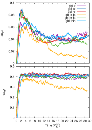
Figure 1: The time evolution of $\langle\alpha_{\rm P}\rangle$ (upper) and $\langle\alpha_{\rm M}\rangle$ (lower) in the global models, where time is in units of the orbital period at a radius of $r=30$, $P^{\rm orb}_{30}$. (For comparison, $P^{\rm orb}_{30}=11.6~{}P^{\rm orb}_{7}$, therefore roughly 370 inner disk orbits are covered.) Details pertaining to the models are listed in Table 1 and corresponding time averaged results are given in Table 2.

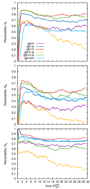
Figure 2: Resolvability (see Eq 21) of the MRI in the global simulations in the $r$ (upper), $\theta$ (middle), and $\phi$-directions (lower).

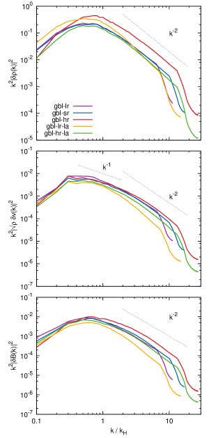
Figure 3: Angle-averaged energy spectrum calculated from time-averaged simulation data showing density (top), kinetic energy (middle), and magnetic energy (lower). The dotted lines are representative power-law slopes (see § 3). The horizontal axis is in units of $k_{\rm H}=2\pi/\langle H\rangle$.

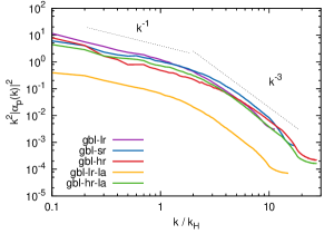
Figure 4: Angle-averaged energy spectrum for the stress-to-gas-pressure ratio, $|\alpha_{\rm p}({\bf k})|^{2}$, calculated from time-averaged simulation data. The horizontal axis is in units of $k_{\rm H}=2\pi/\langle H\rangle$.

3 The quasi-steady state

Following the initial transient phase of evolution, the disk settles into a QSS. In this section we examine the characteristics of this state for the different simulations. We list time and volume averaged parameter values pertaining to the steady-state turbulence in Table 2.

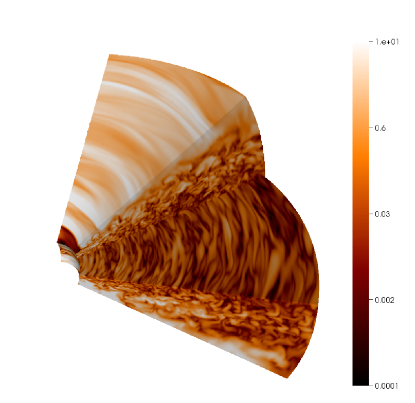
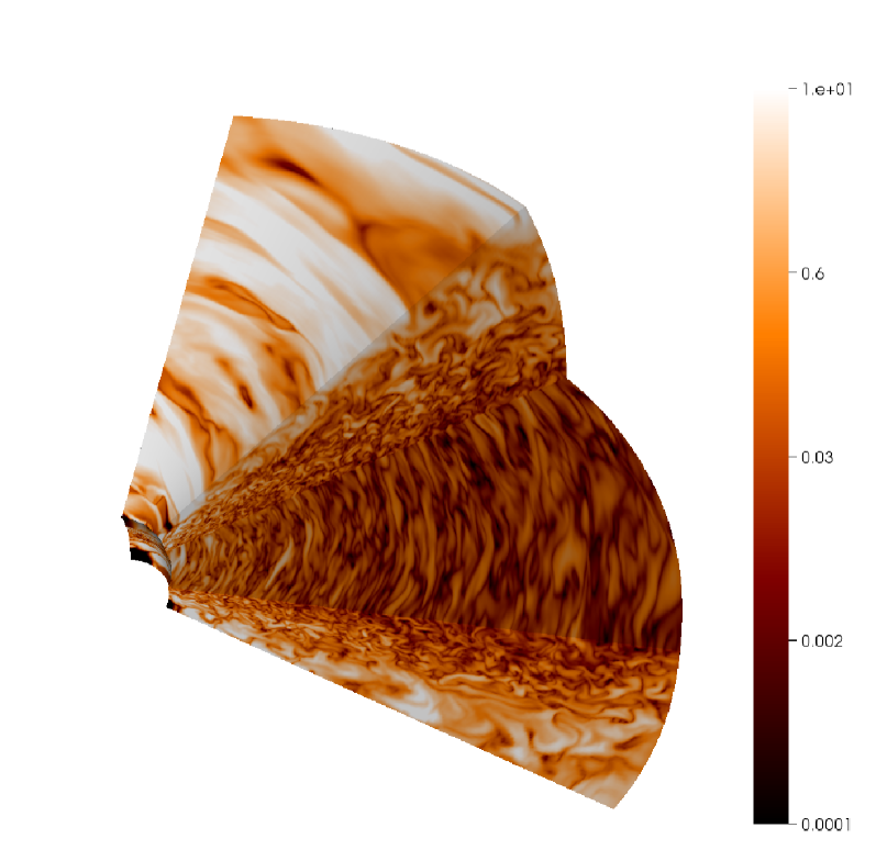
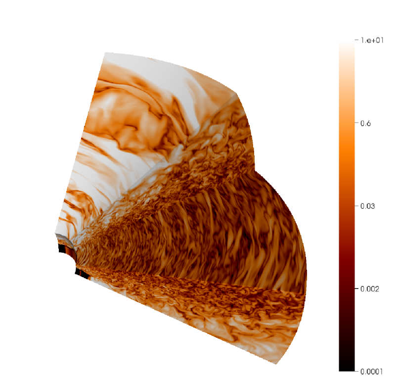
Figure 5: 3D volume rendering showing the ratio of magnetic pressure to gas pressure ($\beta^{-1}$) for models gbl-lr (top), gbl-sr (middle), and gbl-hr (lower). A wedge has been excised from the upper hemisphere of the disk to expose the disk mid-plane.

3.1 Resolution dependence

3.1.1 Convergence: gbl-lr, gbl-sr, and gbl-hr

The volume averaged stress normalised to gas pressure, $\langle\alpha_{\rm P}\rangle$, displays a dependence on resolution in the magnitude of the transient peak at $t\sim 2~{}P^{\rm orb}_{30}$ (Fig. 1). Following this, $\langle\alpha_{\rm P}\rangle$ steadily declines until $t\sim 12~{}P^{\rm orb}_{30}$, at which point the curves level-off and a quasi-steady state is reached. We find a time-averaged value during the quasi-steady state of $\overline{\langle\alpha_{\rm P}\rangle}\simeq 0.04$ for models gbl-lr, gbl-sr, and gbl-hr, indicating convergence with resolution. At the point of convergence, $\overline{\langle\alpha_{\rm P}\rangle}\thinspace\overline{\langle\beta_{\rm d}\rangle}\simeq 0.6$, where $\beta_{\rm d}$ is the disk body plasma-$\beta$. This is in agreement with, but slightly higher than, the relation found for unstratified shearing-box simulations (Sano et al. 2004; Blackman et al. 2008; Guan et al. 2009). The volume averaged Maxwell stress normalised to the magnetic pressure, $\langle\alpha_{\rm M}\rangle$ converges at a value of 0.42 (lower panel of Fig. 1), consistent with previous high resolution stratified shearing box (Hawley et al. 2011; Simon et al. 2012) and global disk models (Parkin & Bicknell 2013).

Convergence in $\overline{\langle\alpha_{\rm P}\rangle}$ is coincident with convergence in the resolvability (Eq 21) - the ability of the numerical grid to resolve the fastest growing MRI modes. Examining Fig. 2, one sees that the $\phi$-direction is the best resolved, followed by the radial direction, and then the $\theta$-direction. At the resolution of model gbl-sr, $N_{\rm r}$ is clearly higher than $N_{\theta}$, suggesting that convergence in global models is tied to the radial magnetic field. That convergence with resolution is more readily achievable for the radial magnetic field is illustrated by the relative magnetic field strengths: $\overline{\langle\beta_{\rm r}\rangle}\simeq 128$, $\overline{\langle\beta_{\theta}\rangle}\simeq 361$, and $\overline{\langle\beta_{\phi}\rangle}\simeq 17$. The converged value for $N_{\phi}$ is roughly 0.8, consistent with some fraction of the disk having weak magnetic fields (due to zero-net flux dynamo oscillations) which have corresponding $\lambda_{\rm MRI}$ values which are below the simulation resolution. Poloidal magnetic fields in our simulations appear relatively strong, with our models returning $\overline{<B_{\rm r}^{2}>/<B_{\phi}^{2}>}=0.13$ and $\overline{<B_{\theta}^{2}>/<B_{\phi}^{2}>}=0.05$ compared to respective values of $\sim 0.08$ and $\sim 0.02$ for the highest resolution model in Hawley et al. (2011). We attribute this difference to the higher resolution used in our models.

Power spectra computed for density, kinetic energy, and total magnetic energy perturbations are shown in Fig. 3. A perturbation for a variable q is calculated by subtracting the azimuthal average, such that $\delta q=q-[q]$. Perturbations are used to reduce the influence of large scale radial and vertical gradients on the resulting power spectra. The position of the low wavenumber turnover between models gbl-lr, gbl-sr, and gbl-hr is consistent at $k/k_{\rm H}\simeq 0.5$, illustrating that the resolution of the largest physical structures is converged. The slope of the magnetic energy power spectrum is approximately $k^{-2}$. This apparent constant power-law slope suggests a self-similar transfer of energy from large to small scales which may indicate an inertial cascade, although it may also be due to the injection of energy by the MRI at all realisable scales (Fromang & Papaloizou 2007). The power spectra for magnetic energy and kinetic energy exhibit very similar shapes. On further inspection one sees that magnetic energy is slightly larger than kinetic energy on length scales of roughly a disk scale-height ($0.4\mathrel{\hbox to0.0pt{\lower 3.0pt\hbox{$\sim$}\hss}\raise 2.0pt\hbox{$<$}}k/k_{\rm H}\mathrel{\hbox to0.0pt{\lower 3.0pt\hbox{$\sim$}\hss}\raise 2.0pt\hbox{$<$}}5$, where $k_{\rm H}=2\pi/\langle H\rangle$), whereas they are approximately equal on the smallest length scales ($k/k_{\rm H}\mathrel{\hbox to0.0pt{\lower 3.0pt\hbox{$\sim$}\hss}\raise 2.0pt\hbox{$>$}}5$). This differs from the stratified shearing-box simulations presented by Johansen et al. (2009), for which kinetic energy was found to dominate over magnetic energy at all but the very largest scales in the box. Comparing to the global models of Beckwith et al. (2011), we note that the low wavenumber turnover for magnetic and kinetic energy arises at a similar value (they find $k/k_{\rm H}\sim 0.3$). However, there is a considerable difference in the amplitudes of kinetic and magnetic energy fluctuations, where Beckwith et al. (2011) find the latter to be an order of magnitude lower than the former. The source of this difference is unclear. However, there are number of differences between our approach and that used by Beckwith et al. (2011) in the calculation of the Fourier transforms and the related power spectra. In calculating the value of a fluctuating quantities $\delta Q$ we have adopted a straightforward approach of subtracting an azimuthally averaged value of $Q$, whereas Beckwith et al. (2011) fit a two-dimensional distribution in the radial and vertical directions, which they then subtract to determine $\delta Q$. Another major difference is that we define a conventional spherical Fourier transform through Eq (22), whereas Beckwith et al. (2011) construct azimuthal averages of fluctuating quantities, define a normalized measure of spatial fluctuations in the $(r,\theta)$ coordinates and then define a Fourier transform in $r$ and $\theta$ treating $r$ and $\theta$ as pseudo-Cartesian coordinates (their equation (15)). A comparison of these two approaches and the implications for comparing computed accretion disk spectra with one another and also with textbook spectra for homogeneous turbulence, is beyond the scope of this paper.

The power spectra all display a pronounced turn-over at high wavenumber, which depends on resolution, and which we interpret as the dissipation scale. Indeed the morphology of the steep, but slightly curved, step at the high wavenumber end of the magnetic energy power spectrum is indicative of a resolved separation between the Ohmic and viscous dissipation scales (see, e.g., Kraichnan & Nagarajan 1967).

Irrespective of resolution, most of the power in $\alpha_{\rm P}$ is on the largest length scales (i.e. at low wavenumber - Fig. 4). In fact, the relatively flat slope to the $\alpha_{\rm P}$ power spectrum indicates that a large amount of power is also contained in moderate length scales. The slope of the power spectrum changes at $k/k_{\rm H}\sim 3$, becoming steeper, and indicating that smaller length scales contribute considerably less to the global stress. Therefore, although magnetic field correlation lengths demonstrate that MRI-driven turbulence is localised (Guan et al. 2009), we find evidence for angular momentum transport being dominated by larger length scales, of size $\mathrel{\hbox to0.0pt{\lower 3.0pt\hbox{$\sim$}\hss}\raise 2.0pt\hbox{$>$}}\langle H\rangle$.

Increasing the simulation resolution permits structure to occupy smaller spatial scales. This is illustrated by the simulation snapshots of $\beta^{-1}$ shown in Fig. 5. As one progresses to higher resolution through models gbl-lr, gbl-sr, and gbl-hr the size of structures get progressively finer. Also, contrasts in the magnetic energy, which are particularly noticeable in the coronal region, become sharper at higher resolution. This equates to an increase in $\nabla\times B$ with resolution, which we examine in more detail in § 4.

In summary, convergence is achieved for a resolution of 12-51 cells/$H$ in radius, 27 cells/$H$ in the $\theta$-direction, and 12.5 cells/$H$ in the $\phi$-direction (model gbl-sr). This is considerably below the 64-128 cells/$H$ required for convergence in stratified shearing box simulations found by Davis et al. (2010), whereas the vertical resolution is comparable to the 25 cells/$H$ necessary to produce sustained turbulence in the models of Fromang & Nelson (2006) and Flock et al. (2011). In § 5 we provide an explanation for this dramatic difference.

3.1.2 Influence of $\phi-resolution$: gbl-lr-la and gbl-hr-la

When the azimuthal field is under-resolved, turbulent activity dies out, as discussed by Fromang & Nelson (2006), Flock et al. (2011), and Parkin & Bicknell (2013). This effect can be seen in the stresses and resolvabilities computed for model gbl-lr-la (a lower azimuthal resolution variant of gbl-lr - see Table 1), which we plot in Figs. 1 and 2. Repeating this experiment at higher resolution (models gbl-hr and gbl-hr-la), one finds that even though the azimuthal field is barely-resolved (8 cells/$H$ in the azimuthal direction for gbl-hr-la), only a slightly lower $\overline{\langle\alpha_{\rm P}\rangle}$ value is obtained. Therefore, we find a similar dependence on azimuthal resolution to that discussed by Hawley et al. (2011), although this dependence appears to become less pronounced at higher resolution, and this is possibly due to compensation by the poloidal grid resolution. This indicates that low azimuthal resolution can, to some extent, be compensated for by higher poloidal resolution. However, based on these results it would seem advisable to adopt an aspect ratio close to unity. We also note that our $\alpha_{\rm P}$ and $\alpha_{\rm M}$ values are higher than in the models of Beckwith et al. (2011) and Hawley et al. (2011). We attribute this to the higher simulation resolution and lower cell aspect ratio used in our models - (see also the discussion in Fromang & Nelson 2006; Flock et al. 2011; Parkin & Bicknell 2013).

As discussed in the previous section, the power spectra in Fig. 3 display a turn-over at high wavenumber corresponding to the dissipation scale. All simulations presented in this paper rely on numerical dissipation, hence one may anticipate that numerical resolution sets this scale and adopting a lower resolution in a certain direction may shift the dissipation scale to lower wavenumbers. Comparing the curves for models gbl-lr and gbl-lr-la in Fig. 3, the slope in the magnetic energy power spectrum is steeper for gbl-lr-la in the wavenumber range $1\mathrel{\hbox to0.0pt{\lower 3.0pt\hbox{$\sim$}\hss}\raise 2.0pt\hbox{$<$}}k/k_{\rm H}\mathrel{\hbox to0.0pt{\lower 3.0pt\hbox{$\sim$}\hss}\raise 2.0pt\hbox{$<$}}6$. This steeper slope is readily understood as a consequence of under-resolving the fastest growing MRI modes in the $\phi$-direction - energy cannot be injected by the MRI if the mode-growth is not resolved. In relation to the discussion in the previous section, this implies that the power-law slope in the magnetic energy power spectrum of model gbl-lr, for example, is a consequence of magnetic energy injection by the MRI and not solely due to an inertial cascade of energy from large to small scales, consistent with results presented by Fromang & Papaloizou (2007) and Johansen et al. (2009) which illustrate the driving of magnetic energy to smaller scales by the MRI.

3.2 Other factors which might affect the saturated state

3.2.1 Gas pressure dependence: gbl-thin

Based on a suite of unstratified shearing-box simulations, Sano et al. (2004) have reported a dependence of the QSS stress level on the gas pressure. To examine whether this dependence exists in global simulations, one can utilise simulations with different aspect ratios because $H/R\propto c_{\rm s}\propto\sqrt{P}$. Models gbl-sr and gbl-thin, which feature $H/R=0.1$ and 0.05, respectively, and an identical number of cells per scale-height in the vertical and azimuthal directions (Table 1), return comparable values of $\overline{\langle\alpha_{\rm P}\rangle}$, with a slightly higher value for the latter (Table 2). Based on the two disk aspect ratios we have explored, there is a weak dependence of $\langle\alpha_{\rm P}\rangle$ on gas pressure. This lack of dependence stems from the similarity in values for the disk body plasma-$\beta$, $\beta_{\rm d}$ (Table 2). Essentially, even though gas pressure is higher in gbl-sr compared to gbl-thin, the relative strength of the Maxwell stresses is very similar.

3.2.2 Initial magnetic field strength

The independence of the saturated state on the initial field strength has been demonstrated by Sano et al. (2004) (zero-net flux, unstratified shearing-boxes), Guan & Gammie (2011) (stratified shearing-boxes), and Hawley et al. (2011) (global stratified disks). In all cases, the dissipation, or expulsion, of the initial magnetic field configuration disconnects its influence from the QSS.

3.2.3 Initial perturbation to the disk

The growth rate of the non-axisymmetric MRI depends on the wavenumber of the initial perturbation (Balbus & Hawley 1992). Faster magnetic field growth arises for higher wavenumbers provided they are sub-critical. Therefore, the growth rate of the stresses in the disk will be higher for higher wavenumber perturbations. Parkin & Bicknell (2013) examined this in the context of global disks, finding that irrespective of the initially excited MRI mode, the onset of non-linear (turbulent) motions in the disk erases the initial perturbation and leads to a statistically similar saturated state.

3.3 Astrophysical implications

Simulations gbl-lr, gbl-sr, and gbl-hr converge at $\overline{\langle\alpha_{\rm P}\rangle}\simeq 0.04$ which should be compared with values of $\sim 0.1-0.3$ commonly derived from relaxation times in post-outburst cataclysmic variables (CVs)(Smak 1999; King et al. 2007; Kotko & Lasota 2012). Although a discrepancy exists, we note that our converged values are consistent with those for isolated AGN disks (Starling et al. 2004). Attaining higher values for $\overline{\langle\alpha_{\rm P}\rangle}$ may, therefore, require the influence of a companion star to be included in simulations. Alternatively, large-scale (net vertical flux) magnetic fields and/or large magnetic Prandtl numbers have been shown to yield larger stresses (Lesur & Longaretti 2007; Fromang et al. 2013; Bai & Stone 2013; Lesur et al. 2013).

4 Control volume analysis

In order to understand the global characteristics of our model accretion disks, we have preformed a control volume analysis of the magnetic energy budget. This involves evaluating terms in the magnetic energy equation integrated over a specific volume, and for this purpose we choose the disk body (defined in § 2.3). The boundaries of this control volume are open in the radial and vertical directions, and periodic in the azimuthal direction.

Previous shearing box simulations show a common characteristic of a consistent power on large scales when convergence is achieved (Simon et al. 2009; Davis et al. 2010). Thus the large scale power in the turbulent spectrum is important when assessing the convergence properties of accretion disk simulations. In turbulent gases (and in our simulations) most of the energy is contained in the largest scales so that our volume-integrated approach to the energy budget is useful in understanding the characteristics of the low wave number part of the spectrum.

Another important aspect of the control volume analysis is that it provides a guide for constraining the various terms describing production, advection, volumetric changes and dissipation in analytic modeles of accretion disks (e.g. Balbus & Papaloizou 1999; Kuncic & Bicknell 2004). For example, this analysis informs us whether the vertical advection of turbulent energy is important compared to the production of turbulence in magnetised disks.

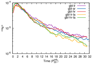
Figure 6: Volume averaged magnetic energy, $\langle u_{\rm B}\rangle$, as a function of time.

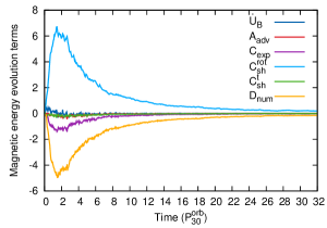
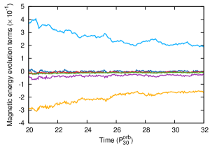
Figure 7: Comparison of terms pertaining to the control volume analysis for model gbl-sr (see § 4.1). The upper and lower panels show results for time intervals 0-32 and $20-32~{}P_{30}^{\rm orb}$, respectively. Rates of change of energy are plotted in units of $1/P_{30}^{\rm orb}$ - to convert to code units divide the values by $P_{30}^{\rm orb}=964$. Note the difference in scale between the plots.

4.1 Magnetic energy evolution

To set the scene, we first examine the control volume averaged magnetic energy, $\langle u_{\rm B}\rangle$ (Fig. 6). The curves follow the general morphology of a rapid rise in $u_{\rm B}$ during the initial transient phase, followed by a similarly rapid fall in magnetic energy which gradually flattens out as the quasi-steady state ($\overline{\partial\langle\alpha_{\rm P}\rangle/\partial t}\rightarrow 0$) is reached. For gbl-sr, for example, the quasi-steady state is reached after $t\simeq 14~{}P^{\rm orb}_{30}$. Subsequently, there is a slow, but steady, decrease in magnetic energy.

We begin with the magnetic field induction equation, to which we add a term for numerical resistivity, $\eta_{\rm num}$, such that Eq (4) now reads,

$$\frac{\partial\bf B}{\partial t}=\nabla\times({\bf v\times B})+\eta_{\rm num}\nabla^{2}{\bf B}.$$ (24)

The motivation for introducing $\eta_{\rm num}$ will become clear in the remainder of the paper. For now we merely note that the truncated order of accuracy of numerical finite volume codes (such as the PLUTO code used in this investigation) brings with it a truncation error which we interpret as a numerical resistivity and which we model with the additional Ohmic term in Eq (24). Taking the scalar product of ${\bf B}$ with Eq (24) and re-arranging terms gives,

$$\frac{\partial u_{\rm B}}{\partial t}=B_{\rm i}B_{\rm j}s_{\rm ij}-\frac{1}{3}u_{\rm B}v_{\rm k,k}-\frac{\partial}{\partial x_{\rm j}}(u_{\rm B}v_{\rm j})+\eta_{\rm num}B_{\rm i}\nabla^{2}B_{\rm i},$$ (25)

where $u_{\rm B}=|B|^{2}/2$, the fluid shear tensor,

$$s_{\rm ij}=\frac{1}{2}(v_{\rm i,j}+v_{\rm j,i}-\frac{2}{3}\delta_{\rm ij}v_{\rm k,k}),$$ (26)

and the Maxwell stress tensor is given by Eq (15), and a subscript comma denotes partial differentiation. Next we expand ${\bf v}={\bf v}^{\rm t}+{\bf v}^{\rm rot}$, where $v^{\rm t}$ is the perturbed velocity field in the rotating frame and,

$${\bf v}^{\rm rot}=v^{\rm rot}\hat{\phi}=[v_{\phi}]\hat{\phi},$$ (27)

is the azimuthally averaged rotational velocity. This step allows the respective contributions to the terms in Eq (25) from the mean background disk rotation and the perturbed velocity field (in the rotating frame) to be inspected. Substituting Eq (27) into Eq (25) and integrating over a control volume $V$ with bounding surface $S$, and using the relation,

$$B_{\rm i}B_{\rm j}s_{\rm ij}-\frac{1}{3}u_{\rm B}v_{\rm k,k}=B_{\rm i}B_{\rm j}v_{\rm i;j}-u_{\rm B}v_{\rm k,k},$$ (28)

to separate shear and expansion terms (where a subscript semi-colon indicates a covariant derivative) one arrives at,

$$\dot{U}_{\rm B}=C^{\rm rot}_{\rm sh}+C^{\rm t}_{\rm sh}+C_{\rm exp}+A_{\rm adv}+D_{\rm num},$$ (29)

where,

$$\dot{U}_{\rm B} = \int\frac{\partial u_{\rm B}}{\partial t}dV,$$ (30)

$$C^{\rm rot}_{\rm sh} = \int B_{\rm i}B_{\rm j}v^{\rm rot}_{\rm i;j}dV,$$ (31)

$$C^{\rm t}_{\rm sh} = \int B_{\rm i}B_{\rm j}v^{\rm t}_{\rm i;j}dV,$$ (32)

$$C_{\rm exp} = -\int u_{\rm B}v^{\rm t}_{\rm k,k}dV,$$ (33)

$$A_{\rm adv} = -\oint u_{\rm B}v^{\rm t}_{\rm j}n_{\rm j}dS,$$ (34)

$$D_{\rm num} = -\eta_{\rm num}\left[\oint\frac{\partial M^{\rm B}_{\rm ij}}{\partial x_{\rm i}}n_{\rm j}dS+\int|j|^{2}dV\right],$$ (35)

and where the current density, $j_{\rm i}=[\nabla\times B]_{\rm i}$, and the Maxwell stress tensor, $M^{\rm B}_{\rm ij}$, is given by (15). All terms featuring in Eqs (29)-(35) are exact and can be explicitly calculated from the simulation data. The numerical resistivity, $\eta_{\rm num}$, is estimated by solving Eq (29) for $D_{\rm num}$ and then solving Eq (35) for $\eta_{\rm num}$. To maintain consistency with the third-order spatial reconstruction used in the simulations, we compute terms appearing in Eqs (29)-(35) to third-order accuracy using reconstruction via the primitive function (see Colella & Woodward 1984; Laney 1998, for further details).

Before proceeding to the results of the control volume analysis, a brief description of the terms and their respective meaning is worthwhile. The volume integrated rate of change of magnetic energy is given by $\dot{U}_{\rm B}$. $C^{\rm rot}_{\rm sh}$ and $C^{\rm t}_{\rm sh}$ are the production of magnetic energy by the shear in the mean disk rotation and the turbulent velocity field, respectively. $C_{\rm exp}$ corresponds to changes in magnetic energy due to expansion in the gas. $A_{\rm adv}$ is a surface term for the advection of magnetic energy in/out of the control volume by the turbulent velocity field. There are contributions to the surface integrals from the radial and $\theta$-direction - periodic boundaries in the azimuthal direction lead to a cancellation, and thus no contribution from those surfaces. (Note that the term $\oint u_{\rm B}v^{\rm rot}_{\rm j}n_{\rm j}dS$ vanishes because of the periodic boundary conditions in the azimuthal direction, therefore the mean disk rotation does not advect magnetic energy in/out of the control volume.) Finally, $D_{\rm num}$ corresponds to numerical dissipation. We note that the value of $D_{\rm num}$ is exact, as it is merely the remainder required to balance the magnetic energy equation (Eq 29). However, our determination of $\eta_{\rm num}$ from $D_{\rm num}$ is not exact in view of our assumed Ohmic form for the numerical resistive term in Eq (24). Nevertheless, we consider this estimate to be indicative of the actual numerical resistivity.

In Fig. 7 we plot the results of applying the control volume analysis to model gbl-sr. One immediately notices that magnetic energy production is dominated by $C^{\rm rot}_{\rm sh}$ (see also discussion in Kuncic & Bicknell 2004) and removal is predominantly via numerical dissipation, $D_{\rm num}$. There is non-negligible magnetic energy removal by divergence in the velocity field ($C_{\rm exp}$). Examining the directional contributions to this term, one finds roughly equal magnitudes for the $r$, $\theta$, and $\phi$ components. However, the poloidal contributions ($r,\theta$) are expansions, which remove magnetic energy, whereas the azimuthal contribution is compressive, thus being a source of magnetic energy. Flow divergence impacting on magnetic field evolution has also been observed in stratified shearing-box simulations by Johansen et al. (2009). The turbulent velocity field does not contribute greatly to magnetic energy production, as is demonstrated by the comparably small values for the $C^{\rm t}_{\rm sh}$ curve. A negligible amount of magnetic energy appears to be advected out of the volume in the radial and vertical directions as shown by the curve for $A_{\rm adv}$, consistent with stable magnetically buoyant (Parker) modes within $|z|<2H$ (Shi et al. 2010). Therefore, although “butterfly” diagrams indicate quasi-periodic vertical magnetic field expulsion (e.g. Gressel 2010), it would seem that a much greater amount of energy is dissipated within the disk body. The rate of change of magnetic energy is relatively small compared to magnetic energy production by $C^{\rm rot}_{\rm sh}$ and dissipation by $D_{\rm num}$. Computing a time-averaged value between orbits 12-32, we find $\overline{\dot{U}_{\rm B}}=-3.5\times 10^{-6}$. Therefore, although $\langle\alpha_{\rm P}\rangle$ exhibits quasi-steady behaviour, $\langle u_{\rm B}\rangle$ is continually declining, but at a constantly decreasing rate.

Examining the dissipation term, $D_{\rm num}$, in more detail, one finds that the first term in square brackets on the RHS of Eq (35) is considerably smaller than the second. This shows that dissipation is primarily powered by the current density, $|j|$. In Fig. 8 we show $\int|j|^{2}dV$. There is a striking similarity between the morphology of the curves in this plot with those for $\langle u_{\rm B}\rangle$ (Fig. 6), suggesting an intimate link between the evolution of the magnetic energy, dissipation driven by a turbulent magnetic field, and magnetic energy production (also demonstrated by $C^{\rm rot}_{\rm sh}$ and $D_{\rm num}$ in Fig. 7). Comparing time-averaged values for $D_{\rm num}$ from models gbl-lr, gbl-sr, and gbl-hr, we find very little difference. Therefore, as convergence with resolution is achieved for $\overline{\langle\alpha_{\rm P}\rangle}$, the level of dissipation also converges. We elaborate on the above points in § 5 in the context of a unified description for the observed evolution in accretion disk simulations.

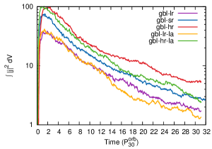
Figure 8: Integral of the current density squared, $|j|^{2}$, over the control volume. This term indicates the level of turbulent activity in the magnetic field and is the dominant contributor to $D_{\rm num}$.

The formulation of the magnetic energy equation used in Eq (29) allows one to distinguish the contributions from shearing and expansions in the disk. However, with a view to understanding the influence of the boundary conditions for the control volume on the magnetic energy, and on the power injected by Maxwell stresses and Lorentz forces, an alternative formulation may be used. To this end we re-cast Eq (29) as:

$$\dot{U}_{\rm B}=C^{\rm rot}_{\rm Lor}+C^{\rm t}_{\rm Lor}+A^{\rm rot}_{\rm MS}+A^{\rm t}_{\rm MS}+A_{\rm adv}+D_{\rm num},$$ (36)

where,

$$C^{\rm rot}_{\rm Lor} = -\int v^{\rm rot}_{\rm i}\frac{\partial M^{\rm B}_{\rm ij}}{\partial x_{\rm j}}dV=-\int v^{\rm rot}_{\rm i}F^{\rm L}_{\rm i}dV,$$ (37)

$$C^{\rm t}_{\rm Lor} = -\int v^{\rm t}_{\rm i}\frac{\partial M^{\rm B}_{\rm ij}}{\partial x_{\rm j}}dV=-\int v^{\rm t}_{\rm i}F^{\rm L}_{\rm i}dV,$$ (38)

$$C_{\rm Lor} = C^{\rm rot}_{\rm Lor}+C^{\rm t}_{\rm Lor},$$ (39)

$$A^{\rm rot}_{\rm MS} = \oint M^{\rm B}_{\rm ij}v^{\rm rot}_{\rm j}n_{\rm i}dS,$$ (40)

$$A^{\rm t}_{\rm MS} = \oint M^{\rm B}_{\rm ij}v^{\rm t}_{\rm j}n_{\rm i}dS,$$ (41)

$$A_{\rm MS} = A^{\rm rot}_{\rm MS}+A^{\rm t}_{\rm MS},$$ (42)

and where $\dot{U}_{\rm B}$, $A_{\rm adv}$, and $D_{\rm num}$ are given by Eqs (30), (34), and (35), respectively. The rates of work done within the control volume by the Lorentz force, $F^{\rm L}$, in combination with the mean disk rotation, $v^{\rm rot}$, and the turbulent velocity field (in the rotating frame), $v^{\rm t}$, are given by $C^{\rm rot}_{\rm Lor}$ and $C^{\rm t}_{\rm Lor}$, respectively. Similarly, the rates of work done on the surfaces of the control volume by combinations of the Maxwell stresses and $v^{\rm rot}$ and $v^{\rm t}$ are, respectively, given by $A^{\rm rot}_{\rm MS}$ and $A^{\rm t}_{\rm MS}$.

In Fig. 9 we show the result of applying Eq (36) to model gbl-sr. Magnetic energy production, which was shown to be predominantly due to $C^{\rm rot}_{\rm sh}$ in Fig. 7, can now be attributed to the rates of work done by the mean disk rotation in combination with Maxwell stresses applied to the boundaries of the volume, $A^{\rm rot}_{\rm MS}$, and Lorentz force acting within the volume, $C^{\rm rot}_{\rm Lor}$. In contrast, the turbulent velocity field acts to remove energy from the control volume, as shown by the terms $A^{\rm t}_{\rm MS}$ and $C^{\rm t}_{\rm Lor}$. Examining $A^{\rm rot}_{\rm MS}$, which involves an integration over the surfaces of the control volume, one finds the magnitude of the radial surface terms to be much greater than from the vertical surfaces and, in particular, the inner radial surface dominates. Therefore, the rate of magnetic energy production is to a large extent due to the difference between the rates of work done on the radial surfaces of the control volume by Maxwell stresses, and by Lorentz forces within the volume.

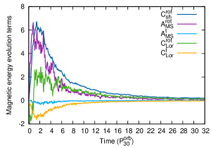
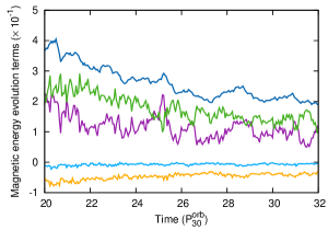
Figure 9: Comparing different terms from the one-zone disk body model for model gbl-sr. The top and bottom panels show results over the time intervals 0-32 and $20-32~{}P_{30}^{\rm orb}$, respectively. Rates of change of energy are plotted in units of $1/P_{30}^{\rm orb}$ - to convert to code units divide the values by $P_{30}^{\rm orb}=964$. Note the difference in scale between the plots.

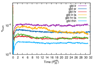
Figure 10: Numerical resistivity, $\eta_{\rm num}$, computed from the control volume analysis (see § 4.1 and 4.2).

Table 3: Time averaged numerical resistivity, $\eta_{\rm num}$, and magnetic Reynolds number, $Re_{\rm M}$. $\eta_{\rm num}$ is estimated using Eq (29) and $Re_{\rm M}=\langle c_{\rm s}H\rangle/\eta_{\rm num}$. $\Delta t_{\rm av}$ (second column) is the time interval over which time averaging was performed.

Model	$\Delta t_{\rm av}$	$\overline{\langle\eta_{\rm num}\rangle}$	$\overline{\langle Re_{\rm M}\rangle}$
gbl-lr	12-31	$1.0\times 10^{-4}$	770
gbl-sr	12-31	$5.8\times 10^{-5}$	1328
gbl-hr	12-31	$3.6\times 10^{-5}$	2139
gbl-lr-la	18-31	$5.8\times 10^{-5}$	1328
gbl-hr-la	12-31	$3.7\times 10^{-5}$	2081
gbl-thin	12-31	$2.5\times 10^{-5}$	1695

4.2 Numerical resistivity

Computing the numerical resistivity, $\eta_{\rm num}$, provides insight into the intrinsic dissipation arising from the simulation method, embodying the truncated order of accuracy present in commonly used numerical schemes. For example, in our present investigation we use third-order accurate spatial reconstruction and second-order accurate time-stepping. Model gbl-sr returns $\overline{\langle\eta_{\rm num}\rangle}=6.1\times 10^{-5}$ and $\overline{\langle Re_{\rm M}\rangle}=1273$, whereas, on the basis of the conclusions drawn by Fleming et al. (2000), Oishi & Mac Low (2011), and Flock et al. (2012b), sustained turbulence should not be observed for $Re_{\rm M}\mathrel{\hbox to0.0pt{\lower 3.0pt\hbox{$\sim$}\hss}\raise 2.0pt\hbox{$<$}}3000$. This disagreement does not appear to be related to our approximation of a constant $\eta_{\rm num}$ throughout the control volume, as tests computed for annuli with radial range $10<r<20$ and $20<r<30$ reveal variations in $\eta_{\rm num}$ of only $5-10\%$. However, it may be due to our assumption that numerical resistivity behaves like an Ohmic resistivity. Previous estimates of numerical resistivity (Fromang & Papaloizou 2007; Simon et al. 2009) adopt a Fourier analysis of the dissipation term whereby $\eta_{\rm num}$ is derived from the high wavenumber end of the spectrum. These analyses reveal that numerical dissipation deviates from Ohmic at low wavenumbers. Our volume averaged values for $\eta_{\rm num}$ provide an estimate which is biased towards the large-scales, and thus may be higher than values at the small scales (i.e. the turbulent dissipation scale). We do note, however, that the third-order accurate spatial reconstruction used in our simulations may allow sustained turbulence at lower $Re_{\rm M}$ than the second-order accuracy used by Flock et al. (2012b). Furthermore, shearing-box boundary conditions suppress terms in the magnetic energy equation that can supply/sustain large scale magnetic fields - the importance of global disk boundary conditions to magnetic field generation is discussed in more detail in § 5.3. Therefore, the large-scale dynamo apparent in stratified global disks (Fig. 11 - see also Arlt & Rüdiger 2001; Fromang & Nelson 2006; O’Neill et al. 2011) may operate effectively at low $Re_{\rm M}$ (Brandenburg 2009; Käpylä & Korpi 2011), meaning that global disks could exhibit sustained turbulence at lower $Re_{\rm M}$ than in a shearing-box (Fleming et al. 2000; Oishi & Mac Low 2011). For further discussion of numerical resistivity see Hirose et al. (2006) and Hawley et al. (2011).

In summary, there are two main reasons for the difference by a factor $\sim 3$ for the critical Reynolds number for the maintenance of turbulence in global disk models compared to the work of Flock et al. (2012b): (1) Differing mathematical approaches to the estimation of the resistivity - Flock et al. (2012b) include an Ohmic resistive term specifically in their simulations, whereas we estimate it using an Ohmic model for the numerical resistivity, (2) The Flock et al. simulations are spatially second order accurate whereas our simulations (and analysis) are spatially third order accurate.

Examining the results for models gbl-lr, gbl-sr, and gbl-hr in Fig. 10 and Table 3, there is the consistent trend that as the resolution is increased (and the cell aspect ratio is kept fixed) the value of $\eta_{\rm num}$ decreases. For example, between models gbl-lr and gbl-sr the resolution has been increased by a factor of 1.5 resulting in a decrease in $\eta_{\rm num}$ by a factor of 1.8. Based on the results for these three simulations we find $Re_{\rm M}\approx 0.45(n_{\rm r})^{1.3}$, where $n_{\rm r}$ is the number of cells in the radial direction, leading to an estimated resolution requirement of $n_{\rm r}\times n_{\theta}\times n_{\phi}\simeq 2600\times 860\times 1000\;$cells to achieve a magnetic Reynolds number, $Re_{\rm M}=10^{4}$. This poses a significant computational challenge. Note that our derived scaling for numerical resistivity is identical to that found by Simon et al. (2009) for unstratified net flux shearing-boxes.

Somewhat surprisingly, model gbl-lr-la displays a lower value for $\eta_{\rm num}$, and thus higher $Re_{\rm M}$, than gbl-lr despite the former having a larger cell aspect ratio. Considering the lower level of turbulent activity in model gbl-lr-la compared to gbl-lr (see Figs. 1 and 8), this shows that numerical resistivity scales with the turbulent motion of the magnetic field, i.e. a larger value of $|j|$ causes a larger net truncation error. In model gbl-lr-la, turbulent activity wanes for $t\mathrel{\hbox to0.0pt{\lower 3.0pt\hbox{$\sim$}\hss}\raise 2.0pt\hbox{$>$}}14~{}P^{\rm orb}_{30}$, and simultaneously the value of $\eta_{\rm num}$ dips (Fig. 10).

5 Boundary conditions and convergence

The question of convergence in simulation studies of magnetized accretion disk turbulence has been long-standing (e.g. Hawley et al. 1995; Stone et al. 1996; Sano et al. 2004; Fromang & Papaloizou 2007; Simon et al. 2009; Guan et al. 2009; Johansen et al. 2009; Davis et al. 2010; Hawley et al. 2011; Sorathia et al. 2012). It is clear that the development, or initial presence, of large-scale magnetic field components is a vital ingredient in enabling convergence with increasing simulation resolution - see the discussion in the second paragraph of § 4. When present, large-scale magnetic fields can replenish low wavenumber magnetic energy. This is a pre-requisite for convergence since otherwise the reservoir of magnetic energy on the largest scales is drained by the turbulent cascading of magnetic energy to smaller scales. We show in this section that the simulation boundary conditions dictate whether large scale mean fields can grow and thereby promote convergence. In doing so, we consider three different classes of simulation: (1) Unstratified shearing boxes; (2) Stratified shearing boxes; (3) Global, stratified disks and (4) Global, unstratified disks. In the simplest case - the unstratified shearing-box with periodic boundary conditions - mean radial and vertical fields cannot readily evolve. When stratification is introduced the associated interface between the disk body and corona, relaxes the constraint on mean radial field growth such that an $\alpha-\Omega$ dynamo can operate effectively. In global models, mean fields grow relatively quickly, enabling large-scale dynamo activity and magnetic energy replenishment. A key result of this analysis is that lower simulation resolution is required in stratified global models compared to shearing-boxes because the large-scale radial gradients enabled by open radial boundaries permit a larger magnitude contribution to the creation of magnetic energy from the Lorentz force terms. Thus, convergence is attained at lower resolutions in global models than in shearing-boxes.

5.1 The magnetic energy balance in accretion disk turbulence

Irrespective of the specific setup (unstratified/stratified shearing box, global simulation) numerical simulations of magnetorotational turbulence exhibit common features. During the early phases of simulation evolution, the MRI develops and the subsequent magnetic field amplification causes a sharp rise in the magnetic energy, $\langle u_{\rm B}\rangle$. Magnetic energy built-up during the initial transient growth phase supports optimal MRI growth and turbulent driving, which in-turn dissipates magnetic energy via the resistivity and the current density, $j_{\rm i}=[\nabla\times B]_{\rm i}$. Magnetic energy subsides, and a state is approached where magnetic field production and turbulent dissipation come into balance. This latter stage is the QSS.

Informed by the analysis in § 4, we write the steady-state magnetic energy evolution equation as (see Eq (36):

$$\dot{U}_{\rm B}=C_{\rm Lor}+A_{\rm MS}+D_{\rm num}\approx 0,$$ (43)

where the separate Lorentz and magnetic stress terms for rotational and turbulent contributions are combined in the following terms:

$$C_{\rm Lor} = -\int v_{\rm i}\frac{\partial M^{\rm B}_{\rm ij}}{\partial x_{\rm j}}dV=-\int v_{\rm i}F^{\rm L}_{\rm i}dV,$$ (44)

$$A_{\rm MS} = \oint M^{\rm B}_{\rm ij}v_{\rm j}n_{\rm i}dS,$$ (45)

where $v_{\rm i}$ is the total (rotational plus turbulent) velocity, $M^{\rm B}_{\rm ij}$ is the Maxwell stress tensor and $F^{\rm L}_{\rm i}$ the Lorentz force. From § 4.1 we have $D_{\rm num}\approx-\eta_{\rm num}\int|j|^{2}dV$, so that Eq (43) for the magnetic energy balance now reads:

$$\oint v_{\rm i}M^{\rm B}_{\rm ij}n_{\rm j}dS-\int v_{\rm i}\frac{\partial M_{\rm ij}^{\rm B}}{\partial x_{\rm j}}\>dV\approx\eta_{\rm num}\int|j|^{2}dV.$$ (46)

Eq (46) states that the achievement of a QSS requires the rate of work done on the surfaces of the control volume by Maxwell stresses, and by Lorentz forces within the volume, to be balanced by dissipation. Magnetic field saturation and the quasi-steady state are solutions to Eq (46).

5.2 Integrated form of the induction equation

In our analysis below, the interplay between the induction equation and the boundary conditions also plays an important role. We begin with the induction equation,

$$\frac{\partial B_{\rm i}}{\partial t}=\frac{\partial}{\partial x_{\rm j}}(v_{\rm i}B_{\rm j}-B_{\rm j}v_{\rm i})+\eta_{\rm num}\nabla^{2}B_{\rm i},$$ (47)

where a numerical resistive term is included for consistency with the magnetic energy balance Eq (46). Integrating Eq (47) over a control volume, $V$, with bounding surface $S$, we have:

$$\frac{\partial}{\partial t}\int B_{\rm i}dV=\oint\left(v_{\rm i}B_{\rm j}-B_{\rm i}v_{\rm j}+\eta_{\rm num}\frac{\partial B_{\rm i}}{\partial x_{\rm j}}\right)\>dS_{\rm j}.$$ (48)

where $dS_{j}$ is the element of surface area and we have assumed $\eta_{\rm num}$ to be approximately spatially constant.

The surface $S$ bounding the control volume as well as the boundary conditions on $S$ take several different forms depending upon the simulation - stratified/unstratified shearing box, stratified/unstratified global disk. However, in general we can use the coordinate convention introduced for shearing boxes (Hawley et al. 1995), adapting the mathematical analysis in each of the different cases. Therefore, the coordinates $x$, $y$ and $z$ correspond to the radial, azimuthal, and vertical directions in the control volume, respectively. The surface integral then involves three separate integrals over the $x$, $y$ and $z$ faces, which we denote by $x=x_{1},\>x_{2}$, $y=y_{1},\>y_{2}$ and $z=z_{1},\>z_{2}$ respectively. In our representation of the integrated induction equation we introduce the resistive flux,

$$F_{i}^{\rm res}=\oint_{S}\eta_{\rm num}\frac{\partial B_{\rm i}}{\partial x_{\rm j}}dS_{\rm j}.$$ (49)

This represents a diffusion of magnetic field, resulting from resistive effects through the bounding surface $S$. The integrated induction equation becomes for each coordinate:

$$\frac{\partial}{\partial t}\int B_{\rm x}dV = F^{\rm res}_{x}+\int_{y_{2}}\left(v_{x}B_{y}-v_{y}B_{x}\right)\>dS_{y}$$ (50)

$$-\int_{y_{1}}\left(v_{x}B_{y}-v_{y}B_{x}\right)\>dS_{y}$$

$$+\int_{z_{2}}\left(v_{x}B_{z}-v_{z}B_{x}\right)\>dS_{z}$$

$$-\int_{z_{1}}\left(v_{x}B_{z}-v_{z}B_{x}\right)\>dS_{z},$$

$$\frac{\partial}{\partial t}\int B_{\rm y}dV = F^{\rm res}_{y}+\int_{x_{2}}\left(v_{y}B_{x}-v_{x}B_{y}\right)\>dS_{x}$$ (51)

$$-\int_{x_{1}}\left(v_{y}B_{x}-v_{x}B_{y}\right)\>dS_{x}$$

$$+\int_{z_{2}}\left(v_{y}B_{z}-v_{z}B_{y}\right)\>dS_{z}$$

$$-\int_{z_{1}}\left(v_{y}B_{z}-v_{z}B_{y}\right)\>dS_{z},$$

$$\frac{\partial}{\partial t}\int B_{\rm z}dV = F^{\rm res}_{z}+\int_{x_{2}}\left(v_{z}B_{x}-v_{x}B_{z}\right)\>dS_{x}$$ (52)

$$-\int_{x_{1}}\left(v_{z}B_{x}-v_{x}B_{z}\right)\>dS_{x}$$

$$+\int_{y_{2}}\left(v_{z}B_{y}-v_{y}B_{z}\right)\>dS_{y}$$

$$-\int_{y_{1}}\left(v_{z}B_{y}-v_{y}B_{z}\right)\>dS_{y}.$$

The surface integrals in Eqs (50) - (52) show the influence of the velocity and magnetic field values at the boundaries on the volume integrated field within the control volume.

5.3 Dependence of convergence on boundary conditions and magnetic field configuration

In the following sections we utilise our description of the magnetic energy balance combined with inferences from the induction equation to describe how the convergence properties of simulations with different numerical setups can be readily understood in terms of the respective boundary conditions and net magnetic field configuration.

5.3.1 Unstratified shearing-box

In this case the model is a periodic box with background shear applied via source terms in the momentum equation. The shearing-box method is used to represent a small patch of an accretion disk in a Cartesian coordinate system such that $x$, $y$, and $z$ correspond to the radial, azimuthal, and vertical directions, respectively; the corresponding lengths of each side of the box are $L_{\rm x}$, $L_{\rm y}$ and $L_{\rm z}$ (see Hawley et al. 1995, for further details). The boundaries of the control volume in this setup are the boundaries of the computational domain. For an unstratified shearing-box, the following shearing-periodic boundary conditions are applied in the radial ($x$), azimuthal ($y$) and vertical ($z$) directions for all dynamical variables $f(x,y,z)$ except the azimuthal velocity. Let $q=d\ln\Omega/d\ln R$ be the shear parameter (=3/2 for a Keplerian disk), then the $x-$, $y-$ and $z-$boundary conditions are:

$$f(x+L_{\rm x},y,z) = f(x,y+q\Omega L_{\rm x}t,z),$$ (53)

$$f(x,y+L_{\rm y},z) = f(x,y,z),$$ (54)

$$f(x,y,z+L_{\rm z}) = f(x,y,z).$$ (55)

The exception is the azimuthal velocity, which satisfies the above $y$- and $z$- boundary conditions but whose $x$-boundary condition is:

$$v_{\rm y}(x+L_{x},y,z)=v_{\rm y}(x,y+q\Omega L_{\rm x}t,z)+q\Omega L_{\rm x}.$$ (56)

Applying these boundary conditions to Eq (46), and noting that $v_{\rm i}B_{\rm i}\approx B_{\rm y}v_{\rm y}$, we have,

$$-q\Omega L_{\rm x}\int_{\rm x_{1}}B_{\rm x}B_{\rm y}dS_{\rm x}+C_{\rm Lor}\approx\eta_{\rm num}\int|j|^{2}dV,$$ (57)

where, as noted, $x_{1}$ refers to the inner radial boundary and $dS_{\rm x}$ is the corresponding element of surface area. Furthermore, noting that structures are typically elongated in the $y$-direction, then $\partial/\partial y\ll\partial/\partial x$ or $\partial/\partial z$, and retaining the largest terms (those linear in $v_{\rm y}$ or $B_{\rm y}$), one finds,

$$-q\Omega L_{\rm x}\int_{\rm x_{1}}B_{\rm x}B_{\rm y}dS_{\rm x}-\int v_{\rm y}B_{\rm x}\frac{\partial B_{\rm y}}{\partial x}dV-\int v_{\rm y}B_{\rm z}\frac{\partial B_{\rm y}}{\partial z}dV$$

$$\approx\eta_{\rm num}\int|j|^{2}dV.$$ (58)

The crucial feature of Eq (58) is that magnetic energy is produced by a combination of the $x-y$ component of the Maxwell stress at the radial boundary and Lorentz forces doing work within the volume; the Lorentz forces depend on the radial and vertical field components as well as the radial and vertical gradient in $B_{\rm y}$. However, the contributions from the second and third terms on the LHS of Eq (58) are negligible on large scales if there is zero-net radial and vertical magnetic field, and/or no radial or vertical gradient in $B_{\rm y}$.

We now consider the implications of the induction equation for the large scale radial and vertical magnetic fields. Inserting the shearing-periodic boundary conditions (53) – (56) into the integrated induction Eqs (50) – (52), we obtain:

$$\frac{\partial}{\partial t}\int B_{\rm x}dV = F^{\rm res}_{\rm x},$$ (59)

$$\frac{\partial}{\partial t}\int B_{\rm y}dV = F^{\rm res}_{y}-q\Omega L_{\rm x}\int_{\rm in}B_{\rm x}dS_{\rm x},$$ (60)

$$\frac{\partial}{\partial t}\int B_{\rm z}dV = F^{\rm res}_{\rm z}.$$ (61)

Eq (60) for the azimuthal field shows that it evolves as a result of resistive diffusion but also, and more importantly as a result of the combined action of velocity shear and the radial field. However, Eq (59) for the integrated radial field and Eq (61) for the vertical field show that these components evolve solely under the action of resistive diffusion and there is no influence from the boundary values of the velocity combined with existing field components. If the net fluxes associated with $B_{x}$ or $B_{z}$ are initially zero and start to build up within the volume then the diffusion terms will act to dissipate these fluxes and they will remain at near zero levels. Hence, initially zero net radial and vertical fields do not develop significant components on the largest scale in the box. On the other hand a net flux vertical field prevails on the timescale of the simulation, and will maintain a component on the largest realizable scale in the simulation domain. This is notwithstanding the effect of diffusion since maintaining a non-zero boundary value of $B_{z}$ minimises diffusion of $B_{z}$ out of the volume as a result of the gradient in $B_{z}$ being close to zero.

Since magnetorotational turbulence extracts energy from the largest scales and drives it towards the smallest scales (Fromang & Papaloizou 2007; Johansen et al. 2009; Lesur & Longaretti 2011), the preservation of a net vertical field fixes the injection of magnetic energy at the scale of the box, thus replenishing the low wavenumber end of the magnetic energy power spectrum. In contrast, in a zero-net flux, unstratified shearing-box, the finite reservoir of magnetic energy at the low wavenumber end of the scale is depleted by turbulent driving.

Achieving convergence is, therefore, related to the presence of magnetic energy injection by Lorentz forces on the largest realisable scales and correspondingly the existence of large scale vertical and/or radial field on those scales. Our analysis explains the results in Simon et al. (2009) who compared zero-net flux and net flux simulations. They demonstrated that energy injection - represented by the Fourier space analogue of our shear term, $C_{\rm sh}^{\rm rot}$ - continues to rise as one tends towards the largest scales in the box in the case of net flux simulations, whereas it plateaus for the zero net flux simulations. This indicates that in evolved zero-net flux turbulence (in an unstratified shearing-box), magnetic energy is not replenished effectively on the largest scales, and this is also consistent with the lack of a large-scale dynamo (Vishniac 2009; Bodo et al. 2011; Käpylä & Korpi 2011).

The above analysis also relates to another well-studied problem within the literature, namely the origin of the lack of convergence with increasing resolution in unstratified, zero-net flux shearing-box simulations (e.g. Fromang & Papaloizou 2007; Pessah et al. 2007; Regev & Umurhan 2008; Vishniac 2009; Käpylä & Korpi 2011; Bodo et al. 2011). As we have shown above, unstratified, zero-net flux shearing-box simulations with periodic boundary conditions render the Lorentz force term ineffective at injecting magnetic energy, and thus a large-scale mean field cannot develop. Hence, when a QSS with turbulent transport of magnetic energy from larger to smaller scales establishes, it must suffice with the largest scale field available: A small-scale dynamo operates, for which the stress scales proportionately to the resistivity (Vishniac 2009; Bodo et al. 2011). Commencing the simulation with a net radial/vertical field (Hawley et al. 1995; Sano et al. 2004; Simon et al. 2009; Guan et al. 2009), or adopting alternative boundary conditions which permit the development of mean fields within a few orbital periods (e.g. vertical field boundary conditions Käpylä & Korpi 2011), enables convergence. Our above analysis provides insight into why these strategies are successful.

5.3.2 Stratified shearing box:

We now consider stratified shearing box simulations in which the vertical component of gravity is included. In the context of the current analysis, the results of zero-net flux simulations by Davis et al. (2010) and Oishi & Mac Low (2011) are useful as periodicity is applied at the boundaries of the computational domain (including the vertical boundary at $|z|=2H$), in common with the unstratified simulations discussed in § 5.3.1. However, unlike the zero-net flux unstratified shearing-boxes described above, the Davis et al. (2010) models converge with increasing resolution. The crucial difference is that stratification provides a means for the disk to repartition magnetic flux so that the disk body can overcome the magnetic flux constraint and generate large scale magnetic fields. In essence, stratification introduces an internal open boundary between the disk body and the coronal region. From the results presented in Davis et al. (2010), we infer this open boundary to lie at $|z_{1,2}|\simeq 1-1.5~{}H$, which we adopt in the following analysis. With the boundaries $z=z_{1}$ and $z=z_{2}$ now not constrained to be periodic the integrated induction equations are:

$$\frac{\partial}{\partial t}\int B_{\rm x}dV = F_{x}^{\rm res}+\int_{z_{2}}v_{\rm x}B_{\rm z}\>dS_{\rm z}-\int_{z_{1}}v_{\rm x}B_{\rm z}\>dS_{\rm z}$$ (62)

$$-\int_{z_{2}}B_{\rm x}v_{\rm z}\>dS_{\rm z}+\int_{z_{1}}B_{\rm x}v_{\rm z}\>dS_{\rm z},$$

$$\frac{\partial}{\partial t}\int B_{\rm y}dV = F_{y}^{\rm res}-q\Omega L_{\rm x}\int_{\rm x_{1}}B_{\rm x}\>dS_{\rm x}$$ (63)

$$+\int_{z_{2}}v_{\rm y}B_{\rm z}\>dS_{\rm z}-\int_{z_{1}}v_{\rm y}B_{\rm z}\>dS_{\rm z}$$

$$-\int_{z_{2}}B_{\rm y}v_{\rm z}\>dS_{\rm z}+\int_{z_{1}}B_{\rm y}v_{\rm z}\>dS_{\rm z},$$

$$\frac{\partial}{\partial t}\int B_{\rm z}dV = F_{z}^{\rm res}.$$ (64)

The non-periodic boundary conditions on the faces $z=z_{1}$ and $z_{2}$ introduce additional driving terms into the radial equation involving the terms $v_{\rm x}B_{\rm z}$ and $B_{\rm x}v_{\rm z}$. Given the zero-net flux condition, these terms are important if the fluctuations in $v_{\rm x}$ and $B_{\rm z}$ or $B_{\rm x}$ and $v_{\rm z}$ are correlated. If this is the case, then Eq (62) opens up the possibility of net radial field development and an $\alpha-\Omega$ dynamo.

Considering the magnetic energy equation, we apply periodic boundaries in the azimuthal and radial directions and an open vertical boundary condition to Eq (46), and retain only the dominant terms, to obtain:

$$-q\Omega L_{\rm x}\int_{\rm x_{1}}B_{\rm x}B_{\rm y}\>dS_{\rm x}+\int_{z_{2}}v_{\rm y}B_{\rm y}B_{\rm z}\>dS_{\rm z}-\int_{z_{1}}v_{\rm y}B_{\rm y}B_{\rm z}\>dS_{\rm z}$$

$$-\int v_{\rm y}B_{\rm z}\frac{\partial B_{\rm y}}{\partial z}dV-\int v_{\rm y}B_{\rm x}\frac{\partial B_{\rm y}}{\partial x}dV\approx\eta_{\rm num}\int|j|^{2}dV.$$ (65)

where the additional term compared to the energy equation for an unstratified disk, Eq (58), arises from the work done on the disk-corona vertical boundary by Maxwell stresses. Despite the presence of the disk-corona interface, a large-scale vertical magnetic field does not develop (see Eq 64). Thus the second, third and fourth terms on the LHS of Eq (65) are negligible. We are left with:

$$-q\Omega L_{\rm x}\int_{\rm x_{1}}B_{\rm x}B_{\rm y}dS_{\rm x}-\int v_{\rm y}B_{\rm x}\frac{\partial B_{\rm y}}{\partial x}dV\approx\eta_{\rm num}\int|j|^{2}dV.$$ (66)

We conjecture that the Davis et al. simulations converge due to the terms involving $B_{\rm x}$ and $B_{\rm y}$ on the LHS of Eq (66), where the introduction of stratification permits the development of a large scale radial magnetic field which combines with the azimuthal field to enable an $\alpha-\Omega$ dynamo to operate. As the simulation resolution is increased, the resolution of MRI modes improves. At a critical resolution, the most unstable wavelength becomes resolved and a further increase in resolution ceases to provide additional MRI growth (because wavelengths shorter than the most unstable mode are stable - Balbus & Hawley 1992, 1998). The contribution to the power input from Maxwell stresses and Lorentz forces (the first and second terms on the LHS of Eq 66) asymptote towards constant values as radial and azimuthal MRI mode growth converges. We note that the above argument is consistent with the results of Oishi & Mac Low (2011), as the presence of a disk-corona interface relaxes the helicity conservation constraint for dynamo quenching.

5.3.3 Global stratified disk simulation

In global stratified disk models, such as the ones we have described in this paper, periodic boundary conditions are applied in the azimuthal direction and the radial and vertical boundaries of the disk body are open. Assuming symmetry about the mid-plane, one may take the vertical surfaces to be anti-periodic. The control volume in our global stratified disk simulations is, in spherical polars, $10\leq r\leq 30$, $\theta_{2H/R}<\theta-\pi/2<\theta_{2H/R}$, where $\theta_{2H/R}=\tan^{-1}(2\langle H/R\rangle)$, and $0\leq\phi\leq\pi/2$. The magnetic energy equation for this control volume, which follows from applying appropriate boundary conditions to the magnetic energy Eq (46) and retaining the dominant terms, is:

$$\int_{r_{2}}B_{\rm r}B_{\phi}v_{\phi}dS_{\rm r}-\int_{r_{1}}B_{\rm r}B_{\phi}v_{\phi}dS_{\rm r}-2\int_{\theta_{1}}B_{\theta}B_{\phi}v_{\phi}dS_{\theta}$$

$$+\>C_{\rm Lor}=\eta_{\rm num}\int|j|^{2}dV,$$ (67)

where the element of volume, $dV=r^{2}\sin\theta drd\theta d\phi$, the surface element orthogonal to $\theta=\rm constant$ is $dS_{\theta}=r\sin\theta drd\phi$, and the surface element orthogonal to $r=\rm constant$ is $dS_{\rm r}=r^{2}d\theta d\phi$. As noted in the last paragraph of § 4.1, the rate of work done by Maxwell stresses on the inner radial boundary is far greater than that done on the outer radial and vertical ($\theta$-direction) boundaries, so that the second term on the LHS of Eq (67) dominates the first and third terms. Also, the largest contributor to $C_{\rm Lor}$ is $\int v_{\phi}B_{\rm r}(\partial B_{\phi}/\partial r)dV$. Hence,

$$-\int_{r_{1}}B_{\rm r}B_{\phi}v_{\phi}dS_{\rm r}-\int v_{\phi}B_{\rm r}\frac{\partial B_{\phi}}{\partial r}dV\simeq\eta_{\rm num}\int|j|^{2}dV.$$ (68)

Note the similarity of the above equation with that governing the stratified shearing-box simulations (Eq 66). The distinct difference is in the magnitude of the terms on the LHS, which depend on $B_{\rm r}$, $B_{\phi}$, and the radial gradient of $B_{\phi}$. Similar to the stratified shearing-box, for magnetic energy production and dissipation to converge, the growth of $B_{\rm r}$ and $B_{\phi}$ must be well resolved. In contrast, however, because of the large-scale radial gradient in $B_{\phi}$ which is present in a global model (see, e.g., figure 12 of Flock et al. 2011) but which is suppressed by periodic radial boundary conditions in a shearing-box, the second term is larger in a global model. This term is appreciable in magnitude for a global disk with open radial and vertical boundaries as a result of the development of a significant net radial field. We can indicate how this arises by considering the integrated induction equation for the radial field, this time in spherical polar coordinates, with periodic azimuthal boundary conditions, viz.,

$$\frac{\partial}{\partial t}\int B_{r}\>dV = \int_{\theta_{2}}(v_{r}B_{\theta}-v_{\theta}B_{r})\>dS_{\theta}$$ (69)

$$-\int_{\theta_{1}}(v_{r}B_{\theta}-v_{\theta}B_{r})\>dS_{\theta}$$

$$\approx-2\int_{\theta_{1}}(v_{r}B_{\theta}-v_{\theta}B_{r})\>dS_{\theta}.$$

In this equation we have omitted the resistive diffusive terms in order to concentrate on the driving terms for $B_{r}$ and we have made use of the approximate anti-symmetry of the $\theta=\theta_{1}$ and $\theta=\theta_{2}$ surfaces.

Returning to the implications for the magnetic energy equation, we note that since periodicity is not applied to Maxwell stresses doing work on the radial boundaries in a global model, they contribute more power. Therefore, in a global model, Lorentz forces within the volume and Maxwell stresses at the boundaries of the disk inject more power at a lower resolutions than they do in a shearing-box. We emphasise that this is the result of radially periodic boundary conditions. Thus, keeping the cell aspect ratio constant and progressively increasing simulation resolution as we have done with models gbl-lr, gbl-sr, and gbl-hr, and as Davis et al. (2010) did with their stratified shearing-box simulations, one should achieve apparent convergence in $\langle\alpha_{\rm P}\rangle$ at lower simulation resolutions (i.e. cells/$H$ in the vertical direction) for global disk simulations than for stratified shearing-box simulations; Davis et al. (2010) found convergence at 64-128 cells/$H$ in the vertical direction, whereas we find convergence at $\sim 27$ cells/$H$ in the vertical direction (see Tables 1 and 2).

Comparing the magnitude of the surface integral terms on the LHS of Eqs (66) and (68), for the magnetic energy of the unstratified shearing-box and global stratified disk respectively, we find that $|\int_{r_{1}}B_{\rm r}B_{\phi}v_{\phi}dS_{\rm r}|$ is greater than $|q\Omega L_{\rm x}\int_{\rm x_{1}}B_{\rm x}B_{\rm y}dS_{\rm x}|$ by a factor of a few tens. Hence, a global disk more readily supports a high $\langle\alpha_{\rm P}\rangle$ because the radial boundary condition allows more power to be delivered to the disk body to counteract the removal of energy by turbulent dissipation ($\eta_{\rm num}\int|j|^{2}dV$). Stating this in a more general context, periodic boundary conditions on the magnetic field prevent the establishment of large-scale gradients in the Maxwell stresses, restricting the power that can be delivered to the disk by Lorentz forces and surface stresses.

We note, however, that in the absence of an explicit resistivity, simulations performed at different resolutions will, at some late time, diverge. This is because in the quasi-steady state the disk is continuing to evolve on the (slow) resistive timescale. If one relies on numerical resistivity, this timescale is dictated by $\eta_{\rm num}$. We anticipate that as global disk simulations integrated over many hundreds of orbits become more feasible, this result will be realised. In fact, the results of Sorathia et al. (2012) already show this for unstratified global disk simulations.

5.3.4 Global unstratified disk simulation

We complete this analysis by considering the global unstratified disk models presented by Sorathia et al. (2012) showing what differences the vertical periodic boundary conditions make in that case. We have presented in Eqs (50) - (52) the volume-integrated induction equations appropriate for Cartesian shearing boxes. Sorathia et al. (2012) employ cylindrical polar coordinates $R,\phi,z$ so that we present the following induction equations in that coordinate system. We are interested in the driving terms for these components so that we omit the diffusive terms in these equations, which have a complex form and do not add anything to the discussion.

The volume-integrated equations, assuming periodicity in the azimuthal direction are:

$$\frac{\partial}{\partial t}\int B_{R}\>dV = \int_{z_{2}}(v_{R}B_{z}-v_{z}B_{R})\>dS_{z}$$ (70)

$$-\int_{z_{1}}(v_{R}B_{z}-v_{z}B_{R})dS_{\rm z},$$

$$\frac{\partial}{\partial t}\int\frac{B_{\phi}}{R}\>dV = \int_{z_{2}}(\frac{v_{\phi}}{R}B_{z}-v_{z}\frac{B_{\phi}}{R})\>dS_{z}$$ (71)

$$-\int_{z_{1}}\left(\frac{v_{\phi}}{R}B_{z}-v_{z}\frac{B_{\phi}}{R}\right)\>dS_{z}$$

$$+\int_{R_{2}}\left(\frac{v_{\phi}}{R}B_{R}-v_{R}\frac{B_{\phi}}{R}\right)\>dS_{R}$$

$$-\int_{R_{1}}\left(\frac{v_{\phi}}{R}B_{R}-v_{R}\frac{B_{\phi}}{R}\right)\>dS_{\rm R},$$

$$\frac{\partial}{\partial t}\int B_{z}\>dV = \int_{R_{2}}(v_{z}B_{R}-v_{R}B_{z})\>dS_{R}$$ (72)

$$-\int_{R_{1}}(v_{z}B_{R}-v_{R}B_{z})\>dS_{\rm R}.$$

where the element of volume $dV=RdRd\phi dz$ and the respective elements of area are $dS_{R}=Rd\phi dz$ (orthogonal to $R=\rm constant$) and $dS_{z}=RdRd\phi$ (orthogonal to $z=\rm constant$). Sorathia et al. (2012) use open radial boundaries and periodic boundary conditions in the vertical and azimuthal direction. Sorathia et al. (2012) use open radial boundaries and periodic boundary conditions in the vertical and azimuthal direction. Since the radial boundaries are open, Eq (72) shows that a mean vertical field can grow irrespective of whether it is initially zero. However, with a periodic $z$-boundary, the RHS of Eq (70) is identically zero and a large scale radial field cannot develop.

Hence, in this case, the magnetic energy equation with only dominant terms retained reads,

$$-\int_{R_{1}}B_{\rm R}B_{\phi}v_{\phi}dS_{\rm R}-\int v_{\phi}B_{\rm R}\frac{\partial B_{\phi}}{\partial R}dV-\int v_{\phi}B_{\rm z}\frac{\partial B_{\phi}}{\partial z}dV$$

$$\simeq\eta_{\rm num}\int|j|^{2}dV,$$ (73)

where we have adopted cylindrical coordinates ($R,\phi,z$) for consistency with the work of Sorathia et al. (2012). The second and third terms in this equation are likely to be small compared to the first (and will contribute little to maintaining magnetic power on the largest scales), because there is no large-scale radial field, and because the disk is unstratified so that there is no appreciable vertical gradient in $B_{\phi}$. Hence, Eq (74) simplifies to,

$$-\int_{\rm R_{1}}B_{\rm R}B_{\phi}v_{\phi}dS_{\rm R}\simeq\eta_{\rm num}\int|j|^{2}dV,$$ (74)

where the remaining Maxwell stress term provides the power input on the largest scales. Note that this term does not require a large-scale net/mean radial field, and has a considerable magnitude purely due to open radial boundary conditions causing a contrast in surface integrals at opposing boundaries. The apparent convergence in $\langle\alpha_{\rm P}\rangle$ present in the results of Sorathia et al. (2012) therefore hinges on adequate resolution of the radial and azimuthal magnetic field. Hence, one may anticipate that stratified and unstratified global models will converge at the same resolution. This is apparent from a comparison of our results with those of Sorathia et al. (2012).

It is noteworthy that although stratified and unstratified global models do appear to converge at similar resolutions, this may be facilitated by different mechanisms in each case. Essentially, because a mean radial field cannot develop in an unstratified global model, maintenance of large scale magnetic energy is not facilitated by a large-scale $\alpha-\Omega$ dynamo, but must be aided by some other mechanism - see, for example, Lesur & Ogilvie (2008). Hence, by construction, periodic vertical boundary conditions place more demand on the azimuthal and vertical fields to sustain turbulent energy on the largest scales. Considering that astrophysical disks are stratified, this seems an unrealistic approximation to a real disk.

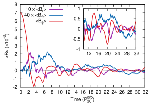
Figure 11: Volume-averaged magnetic field components for model gbl-sr. Note that $\langle B_{\rm r}\rangle$ and $\langle B_{\theta}\rangle$ have been multiplied by factors of 10 and 40, respectively, to aid comparison against the curve for $\langle B_{\phi}\rangle$.

5.4 The presence of a dynamo

The time variability of the mean magnetic field components (Fig. 11) is indicative of an $\alpha-\Omega$ dynamo in our stratified global disk models. Furthermore, mean radial and vertical fields develop within the first few orbital periods of the simulation. The radial and azimuthal mean magnetic fields show anti-correlated oscillations, the period of which is not obvious from Fig. 11. This may be the result of averaging over a wide range of radii (O’Neill et al. 2011), or could be due to additional terms contributing to the evolution of the mean fields when the boundaries of the disk body are open - see the integrated induction equations in § 5.3.3. A connection between the vertical magnetic field and the radial and azimuthal fields is less apparent, although there is a faint suggestion of oscillations in $\langle B_{\theta}\rangle$ with a period on the order of $\sim 15~{}P^{\rm orb}_{30}$.

6 Conclusions

Global three-dimensional simulations of magnetorotationally turbulent disks have been presented to investigate convergence with increasing simulation resolution, magnetic energy, and quasi-steady self-sustaining turbulence. A primary result of this work is convergence with increasing resolution at an $\alpha$-parameter, $\overline{\langle\alpha_{\rm P}\rangle}=0.04$, occurring at a resolution of the order of 12-51 cells/$H$ in radius, 27 cells/$H$ in the vertical direction, and 12.5 cells/$H$ in the azimuthal direction.

A control volume analysis applied to the body of the disk reveals the dominant magnetic energy production to be the result of the combination of Maxwell stresses and shear in the mean disk rotation. Magnetic energy is primarily removed by dissipation, with a negligible amount of energy being advected out of the disk body in either the radial or vertical directions. Compressibility, or to be more exact expansion, also contributes to the removal of magnetic energy, but to a far lesser extent than dissipation. The control volume analysis also allows the numerical resistivity of the simulation code to be evaluated. The results reveal that sustained, slowly diminishing turbulence can operate at $Re_{\rm M}\mathrel{\hbox to0.0pt{\lower 3.0pt\hbox{$\sim$}\hss}\raise 2.0pt\hbox{$<$}}3000$, in contrast to the conclusions of Fleming et al. (2000), Oishi & Mac Low (2011), and Flock et al. (2012b) that magnetorotational turbulence should cease to function effectively at such values of $Re_{\rm M}$. This may be indicating that an effective large-scale dynamo can operate at low magnetic Reynolds number in global disks.

The convergence with resolution found from our global simulations occurs at roughly a factor of three lower resolution than found for stratified shearing-box simulations by Davis et al. (2010) (see also Shi et al. 2010; Hawley et al. 2011, and references there-in). We have shown how this result, as well as the convergence properties of unstratified shearing-boxes (Fromang & Papaloizou 2007; Simon et al. 2009; Guan et al. 2009) and global disks (Hawley et al. 2011; Sorathia et al. 2012) can be understood in terms of balancing creation and dissipation of magnetic energy subject to boundary conditions and magnetic field configuration. In particular, using periodic boundary conditions in the radial direction (as in shearing-box simulations) reduces the magnitude of a Lorentz force term which depends on $B_{\rm r}$ and the radial gradient in $B_{\phi}$. This term significantly contributes to magnetic energy injection, and in global models (which use open radial boundaries) is larger due to the presence of large scale radial gradients. Hence, this term requires lower simulation resolution to achieve the same power in a global model. Our results highlight important differences between shearing-boxes and global disks which indicate the importance of basing future deductions on stratified global models.

In closing we note that the results of this paper concern global disks with a small net vertical magnetic field in the turbulent state. A growing number of shearing-box studies are engaging in the challenging task of modelling net flux magnetic fields in stratified disks (Suzuki & Inutsuka 2009; Suzuki et al. 2010; Moll 2012; Fromang et al. 2013; Bai & Stone 2013; Lesur et al. 2013). Therefore, re-visiting the analysis in this paper in the context of net vertical flux fields would be a useful avenue for future work. Furthermore, the control volume analysis we have used to derive the numerical resistivity could be applied to recent orbital advection/FARGO schemes (e.g. Johansen et al. 2009; Stone & Gardiner 2010; Sorathia et al. 2010; Mignone et al. 2012) to quantify their dissipation properties.

Acknowledgements

We thank the anonymous referee for a useful report. This research was supported under the Australian Research Council’s Discovery Projects funding scheme (project number DP1096417). E. R. P thanks the ARC for funding through this project. This work was supported by the NCI Facility at the ANU and by the iVEC facility at the Pawsey Centre, Perth, WA.

Appendix A Fourier transform in spherical coordinates

The simulations performed in this work use spherical polar coordinates, so for consistency it is best to also perform the Fourier transform in this coordinate system. We adopt spherical polars in real space $(r,\theta,\phi)$ and in Fourier space $(k,\chi,\psi)$. That is,

$$\begin{array}[]{r c l r c l r c l}x&=&r\sin\theta\cos\phi,&k_{x}&=&k\sin\chi\cos\psi,\\ y&=&r\sin\theta\sin\phi,&k_{y}&=&k\sin\chi\sin\psi,\\ z&=&r\cos\theta,&k_{z}&=&k\cos\chi.\end{array}$$ (78)

The following treatment is based on Baddour (2010) with minor differences (primarily the notation of angles and the sign of $\bf k\cdot x$ in the forward and inverse transforms).

A.1 3D Fourier transform

The Fourier transform of a function $f({\bf x})=f(r,\theta,\phi)$ is

$$F({\bf k})=F(k,\chi,\psi)=\int_{0}^{2\pi}\int_{0}^{\pi}\int_{0}^{\infty}f(r,\theta,\phi)\,e^{i{\bf k\cdot x}}\times$$

$$r^{2}\sin\theta\,dr\,d\theta\,d\phi.$$ (79)

Note that we use $e^{i\bf k\cdot x}$ here since this is consistent with many definitions of the Fourier transform.

To proceed, both $e^{i{\bf k\cdot x}}$ and $f$ are expanded in terms of spherical harmonics, which are defined by:

$$Y_{l}^{m}(\theta,\phi)=\sqrt{\frac{(2l+1)(l-m)!}{4\pi(l+m)!}}\,P_{l}^{m}(\cos\theta)\,e^{im\phi},$$ (80)

where the $P_{l}^{m}(\cos\theta)$ are Legendre polynomials.

Let $j_{l}(z)$ be the spherical Bessel function of order $l$, then, denoting complex conjugates by *,

$$e^{i{\bf k\cdot x}}=4\pi\sum_{l=0}^{\infty}\sum_{m=-l}^{l}i^{l}\,j_{l}(kr){Y_{l}^{m}}^{*}(\theta,\phi)Y_{l}^{m}(\chi,\psi),$$ (81)

and,

$$f(r,\theta,\phi)=\sum_{l=0}^{\infty}\sum_{m=-l}^{l}f_{l}^{m}(r)Y_{l}^{m}(\theta,\phi),$$ (82)

where,

$$f_{l}^{m}(r)=\int_{0}^{2\pi}\int_{0}^{\pi}f(r,\theta,\phi)\,{Y_{l}^{m}}^{*}(\theta,\phi)\>\sin\theta\,d\theta\,d\phi,$$ (83)

are the spherical harmonic coefficients of $f(r,\theta,\phi)$.

With these expressions, the Fourier transform is:

$$F(k,\chi,\psi) = 4\pi\int_{0}^{2\pi}\int_{0}^{\pi}\int_{0}^{\infty}\left\{\sum_{l=0}^{\infty}\sum_{m=-l}^{l}f_{l}^{m}(r)Y_{l}^{m}(\theta,\phi)\right.$$ (84)

$$\times\left.\sum_{l^{\prime}=0}^{\infty}\sum_{m^{\prime}=-l^{\prime}}^{l^{\prime}}i^{l^{\prime}}j_{l^{\prime}}(kr){Y_{l^{\prime}}^{m^{\prime}}}^{*}(\theta,\phi){Y_{l^{\prime}}^{m^{\prime}}}(\chi,\psi)\right\}$$

$$\times r^{2}\,\sin\theta\,d\theta\,d\phi.$$

Using the orthogonality property of the spherical harmonics:

$$\int_{0}^{2\pi}\int_{0}^{\pi}Y_{l}^{m}(\theta,\phi)\,{Y_{l^{\prime}}^{m^{\prime}}}^{*}(\theta,\phi)\,\sin\theta\,d\theta\,d\phi=\delta_{ll^{\prime}}\,\delta_{mm^{\prime}},$$ (85)

we obtain,

$$F(k,\chi,\psi) = 4\pi\sum_{l=0}^{\infty}\sum_{m=-l}^{l}F_{l}^{m}(k)\,Y_{l}^{m}(\chi,\psi)$$ (86)

$$\hbox{where,}\qquad F_{l}^{m}(k) = \int_{0}^{\infty}i^{l}r^{2}j_{l}(kr)f_{l}^{m}(r)\>dr,$$ (87)

and the spherical harmonic coefficients $f_{l}^{m}(r)$ are given by equation (83). The steps in evaluating the Fourier transform are:

1. [i)]

2. Evaluate Eq (83) for the spherical harmonic transform, $f(r,\theta,\phi)\Rightarrow f_{\rm l}^{\rm m}(r)$.

3. Perform a spherical Bessel transform using Eq (87), $f_{\rm l}^{\rm m}(r)\Rightarrow F_{\rm l}^{\rm m}(k)$.

4. The $F_{l}^{m}(k)$ are the complete set of Fourier coefficients and can be used to compute an angle averaged spectrum (§ A.2). One may perform an inverse spherical harmonic transform to acquire $F_{\rm l}^{\rm m}(k)\Rightarrow F(k,\chi,\psi)$ using Eq. (86).

For step 1 above we use the publicly available S2kit package which includes functions for performing spherical harmonic transforms on the 2-sphere using a combination of fast-Fourier transforms and fast-Cosine transforms (to tackle the Legendre polynomials) and is based on the seminal work by Driscoll & Healy (1994) (see also Healy et al. 2003). The spherical Bessel transform is computed using numerical quadrature in combination with a truncation of terms contributing at large order $l$ to improve efficiency (§ A.3).

A.2 Angle-averaged spectrum

In the analysis of turbulence, one often uses the integrated energy spectrum:

$$\Pi(k)=\int_{0}^{2\pi}\int_{0}^{\pi}F({\bf k})F^{*}({\bf k})k^{2}\>\sin\chi\,d\chi\,d\psi.$$ (88)

Expressing $F({\bf k})$ in terms of the spherical harmonic expansion (86), we have,

$$\Pi(k) = \int_{0}^{2\pi}\int_{0}^{\pi}\sum_{l=0}^{B}\sum_{|m|\leq l}\,\sum_{p=0}^{B}\sum_{|q|\leq p}F_{l}^{m}(k){F_{p}^{q}}^{*}(k)$$ (89)

$$\times Y_{l}^{m}(\chi,\psi){Y_{p}^{q}}^{*}(\chi,\psi)\>\sin\chi\,d\chi\,d\psi$$

$$= \sum_{l=0}^{B}\sum_{|m|\leq l}F_{l}^{m}(k){F_{l}^{m}}^{*}(k),$$ (90)

with the last equation resulting from the orthogonality of the spherical harmonics (Eq 85).

A.3 Spherical Bessel functions for large $l$

Eq (87), which defines the $k$-dependence of the Fourier coefficients, depends upon integration of the spherical harmonic coefficients with the spherical Bessel functions $j_{l}(kr)$. These have an interesting behaviour at large $l$; they are practically zero until $kr\sim l$ following which they oscillate rapidly. The oscillatory behaviour originates from the expression for the spherical Bessel functions in terms of derivatives of the sinc function, viz.

$$j_{n}(z)=(-1)^{n}z^{n}\left(\frac{1}{z}\frac{d}{dz}\right)^{n}\,\frac{\sin z}{z}$$ (91)

That $j_{l}(kr)\approx 0$ for $kr\ll l$ follows from the leading term:

$$j_{n}(z)=\frac{2^{n}n!}{(2n+1)!}\,z^{n}+{\cal O}z^{n+1}$$ (92)

For what value of $z$ does $j_{n}(z)$ attain a numerically significant value of, say, $\epsilon\sim 10^{-6}$? Take the logarithm of equation (92):

$$\ln j_{n}(z)\approx n\ln 2+n\ln z+\ln n!-\ln(2n+1)!$$ (93)

and use Stirling’s asymptotic form for the factorial function:

$$\ln n!\sim n\ln n-n$$ (94)

to obtain

$$\ln j_{n}(z) \approx n\ln 2+n\ln z+n\ln n$$

$$-(2n+1)\ln(2n+1)+n+1$$

$$= \ln\epsilon$$

$$\Rightarrow\ln z(\epsilon) \approx \frac{1}{n}\ln\epsilon-\ln 2+\frac{(2n+1)}{n}\ln(2n+1)$$ (96)

$$-\ln n-\frac{n+1}{n}$$

For example, for $\epsilon=10^{-6}$ and $n=100$, $\ln z\approx 4.213$ and $z=67.57$.

References

- Arlt & Rüdiger (2001) Arlt, R. & Rüdiger, G. 2001, A&A, 374, 1035
- Armitage et al. (2001) Armitage, P. J., Reynolds, C. S., & Chiang, J. 2001, ApJ, 548, 868
- Baddour (2010) Baddour, N. 2010, Journal of the Optical Society of America A, 27, 2144
- Bai & Stone (2013) Bai, X.-N. & Stone, J. M. 2013, ApJ, 767,30
- Balbus & Hawley (1992) Balbus, S. A. & Hawley, J. F. 1992, ApJ, 400, 610
- Balbus & Hawley (1998) Balbus, S. A. & Hawley, J. F. 1998, Reviews of Modern Physics, 70, 1
- Balbus & Papaloizou (1999) Balbus, S. A. & Papaloizou, J. C. B. 1999, ApJ, 521, 650
- Beckwith et al. (2011) Beckwith, K., Armitage, P. J., & Simon, J. B. 2011, MNRAS, 416, 361
- Beckwith et al. (2008) Beckwith, K., Hawley, J. F., & Krolik, J. H. 2008, ApJ, 678, 1180
- Blackman et al. (2008) Blackman, E. G., Penna, R. F., & Varnière, P. 2008, NewA, 13, 244
- Bodo et al. (2011) Bodo, G., Cattaneo, F., Ferrari, A., Mignone, A., & Rossi, P. 2011, ApJ, 739, 82
- Brandenburg (2005) Brandenburg, A. 2005, Astronomische Nachrichten, 326, 787
- Brandenburg (2009) Brandenburg, A. 2009, ApJ, 697, 1206
- Brandenburg et al. (1995) Brandenburg, A., Nordlund, A., Stein, R. F., & Torkelsson, U. 1995, ApJ, 446, 741
- Colella & Woodward (1984) Colella, P. & Woodward, P. R. 1984, J. Comput. Phys, 54, 174
- Davis et al. (2010) Davis, S. W., Stone, J. M., & Pessah, M. E. 2010, ApJ, 713, 52
- Driscoll & Healy (1994) Driscoll, J. R. & Healy, D. M. 1994, Adv. Appl. Math., 15, 202
- Fleming et al. (2000) Fleming, T. P., Stone, J. M., & Hawley, J. F. 2000, ApJ, 530, 464
- Flock et al. (2012a) Flock, M., Dzyurkevich, N., Klahr, H., Turner, N., & Henning, T. 2012a, ApJ, 744, 144
- Flock et al. (2011) Flock, M., Dzyurkevich, N., Klahr, H., Turner, N. J., & Henning, T. 2011, ApJ, 735, 122
- Flock et al. (2012b) Flock, M., Henning, T., & Klahr, H. 2012b, ApJ, 761, 95
- Fromang (2010) Fromang, S. 2010, A&A, 514, L5
- Fromang et al. (2013) Fromang, S., Latter, H. N., Lesur, G., & Ogilvie, G. I. 2013, A&A, 552, 71
- Fromang & Nelson (2006) Fromang, S. & Nelson, R. P. 2006, A&A, 457, 343
- Fromang & Nelson (2009) Fromang, S. & Nelson, R. P. 2009, A&A, 496, 597
- Fromang & Papaloizou (2007) Fromang, S. & Papaloizou, J. 2007, A&A, 476, 1113
- Fromang et al. (2007) Fromang, S., Papaloizou, J., Lesur, G., & Heinemann, T. 2007, A&A, 476, 1123
- Gardiner & Stone (2008) Gardiner, T. A. & Stone, J. M. 2008, J. Comput. Phys, 227, 4123
- Gressel (2010) Gressel, O. 2010, MNRAS, 405, 41
- Guan & Gammie (2011) Guan, X. & Gammie, C. F. 2011, ApJ, 728, 130
- Guan et al. (2009) Guan, X., Gammie, C. F., Simon, J. B., & Johnson, B. M. 2009, ApJ, 694, 1010
- Hawley (2000) Hawley, J. F. 2000, ApJ, 528, 462
- Hawley (2001) Hawley, J. F. 2001, ApJ, 554, 534
- Hawley et al. (1995) Hawley, J. F., Gammie, C. F., & Balbus, S. A. 1995, ApJ, 440, 742
- Hawley et al. (2011) Hawley, J. F., Guan, X., & Krolik, J. H. 2011, ApJ, 738, 84
- Hawley & Krolik (2001) Hawley, J. F. & Krolik, J. H. 2001, ApJ, 548, 348
- Healy et al. (2003) Healy, D. M., Rockmore, D., Kostelec, P., & Moore, S. 2003, The Journal of Fourier Analysis and Applications, 9, 341
- Heinemann & Papaloizou (2009) Heinemann, T. & Papaloizou, J. C. B. 2009, MNRAS, 397, 64
- Hirose et al. (2006) Hirose, S., Krolik, J. H. & Stone, J. M. 2006, ApJ, 640, 901
- Johansen et al. (2009) Johansen, A., Youdin, A., & Klahr, H. 2009, ApJ, 697, 1269
- Käpylä & Korpi (2011) Käpylä, P. J. & Korpi, M. J. 2011, MNRAS, 413, 901
- King et al. (2007) King, A. R., Pringle, J. E., & Livio, M. 2007, MNRAS, 376, 1740
- Kotko & Lasota (2012) Kotko, I. & Lasota, J.-P. 2012, A&A, 545, A115
- Kraichnan & Nagarajan (1967) Kraichnan, R. H. & Nagarajan, S. 1967, Physics of Fluids, 10, 859
- Kuncic & Bicknell (2004) Kuncic, Z. & Bicknell, G. V. 2004, ApJ, 616, 669
- Laney (1998) Laney, C. B. 1998, Computational Gasdynamics, Cambridge University Press
- Latter et al. (2009) Latter, H. N., Lesaffre, P., & Balbus, S. A. 2009, MNRAS, 394, 715
- Latter & Papaloizou (2012) Latter, H. N. & Papaloizou, J. C. B. 2012, MNRAS, 426, 1107
- Lesaffre et al. (2009) Lesaffre, P., Balbus, S. A., & Latter, H. 2009, MNRAS, 396, 779
- Lesur et al. (2013) Lesur, G., Ferreira, J., & Ogilvie, G. I. 2013, A&A, 550, A61
- Lesur & Longaretti (2007) Lesur, G. & Longaretti, P.-Y. 2007, MNRAS, 378, 1471
- Lesur & Longaretti (2011) Lesur, G. & Longaretti, P.-Y. 2011, A&A, 528, A17
- Lesur & Ogilvie (2008) Lesur, G. & Ogilvie, G. I. 2008, A&A, 488, A451
- Lyra et al. (2008) Lyra, W., Johansen, A., Klahr, H., & Piskunov, N. 2008, A&A, 479, 883
- McKinney et al. (2012) McKinney, J. C., Tchekhovskoy, A., & Blandford, R. D. 2012, MNRAS, 423, 3083
- Mignone et al. (2007) Mignone, A., Bodo, G., Massaglia, S., Matsakos, T., Tesileanu, O., Zanni, C., & Ferrari, A. 2007, ApJS, 170, 228
- Mignone et al. (2012) Mignone, A., Flock, M., Stute, M., Kolb, S. M., & Muscianisi, G. 2012, A&A, 545, A152
- Miller & Stone (2000) Miller, K. A. & Stone, J. M. 2000, ApJ, 534, 398
- Miyoshi & Kusano (2005) Miyoshi, T. & Kusano, K. 2005, J. Comput. Phys, 208, 315
- Moll (2012) Moll, R. 2012, A&A, 548, A76
- Nelson & Gressel (2010) Nelson, R. P. & Gressel, O. 2010, MNRAS, 409, 639
- Noble et al. (2010) Noble, S. C., Krolik, J. H., & Hawley, J. F. 2010, ApJ, 711, 959
- Oishi & Mac Low (2011) Oishi, J. S. & Mac Low, M.-M. 2011, ApJ, 740, 18
- O’Neill et al. (2011) O’Neill, S. M., Reynolds, C. S., Miller, M. C., & Sorathia, K. A. 2011, ApJ, 736, 107
- Paczyńsky & Wiita (1980) Paczyńsky, B. & Wiita, P. J. 1980, A&A, 88, 23
- Parkin & Bicknell (2013) Parkin, E. R. & Bicknell, G. V. 2013, ApJ, 763, 99
- Pessah et al. (2007) Pessah, M. E., Chan, C.-k., & Psaltis, D. 2007, ApJL, 668, L51
- Pringle (1981) Pringle, J. E. 1981, ARA&A, 19, 137
- Regev & Umurhan (2008) Regev, O. & Umurhan, O. M. 2008, A&A, 481, 21
- Rider et al. (2007) Rider, W. J., Greenough, J. A., & Kamm, J. R. 2007, J. Comput. Phys, 225, 1827
- Sano et al. (2004) Sano, T., Inutsuka, S.-i., Turner, N. J., & Stone, J. M. 2004, ApJ, 605, 321
- Shakura & Sunyaev (1973) Shakura, N. I. & Sunyaev, R. A. 1973, A&A, 24, 337
- Shi et al. (2010) Shi, J., Krolik, J. H., & Hirose, S. 2010, ApJ, 708, 1716
- Simon et al. (2012) Simon, J. B., Beckwith, K., & Armitage, P. J. 2012, MNRAS, 422, 2685
- Simon et al. (2009) Simon, J. B., Hawley, J. F., & Beckwith, K. 2009, ApJ, 690, 974
- Simon et al. (2011) Simon, J. B., Hawley, J. F., & Beckwith, K. 2011, ApJ, 730, 94
- Smak (1999) Smak, J. 1999, AcA, 49, 391
- Sorathia et al. (2010) Sorathia, K. A., Reynolds, C. S., & Armitage, P. J. 2010, ApJ, 712, 1241
- Sorathia et al. (2012) Sorathia, K. A., Reynolds, C. S., Stone, J. M., & Beckwith, K. 2012, ApJ, 749, 189
- Starling et al. (2004) Starling, R. L. C., Siemiginowska, A., Uttley, P., & Soria, R. 2004, MNRAS, 347, 67
- Stone & Gardiner (2010) Stone, J. M. & Gardiner, T. A. 2010, ApJS, 189, 142
- Stone et al. (1996) Stone, J. M., Hawley, J. F., Gammie, C. F., & Balbus, S. A. 1996, ApJ, 463, 656
- Suzuki & Inutsuka (2009) Suzuki, T. K. & Inutsuka, S. -i. 2009, ApJ, 691, L49
- Suzuki et al. (2010) Suzuki, T. K., Muto,T., & Inutsuka, S. -i 2010, ApJ, 718, 1289
- Vishniac (2009) Vishniac, E. T. 2009, ApJ, 696, 1021