CSMA using the Bethe Approximation: Scheduling and Utility Maximization

Abstract

CSMA (Carrier Sense Multiple Access), which resolves contentions over wireless networks in a fully distributed fashion, has recently gained a lot of attentions since it has been proved that appropriate control of CSMA parameters guarantees optimality in terms of stability (i.e., scheduling) and system-wide utility (i.e., scheduling and congestion control). Most CSMA-based algorithms rely on the popular MCMC (Markov Chain Monte Carlo) technique, which enables one to find optimal CSMA parameters through iterative loops of ‘simulation-and-update’. However, such a simulation-based approach often becomes a major cause of exponentially slow convergence, being poorly adaptive to flow/topology changes. In this paper, we develop distributed iterative algorithms which produce approximate solutions with convergence in polynomial time for both stability and utility maximization problems. In particular, for the stability problem, the proposed distributed algorithm requires, somewhat surprisingly, only one iteration among links. Our approach is motivated by the Bethe approximation (introduced by Yedidia, Freeman and Weiss [1]) allowing us to express approximate solutions via a certain non-linear system with polynomial size. Our polynomial convergence guarantee comes from directly solving the non-linear system in a distributed manner, rather than multiple simulation-and-update loops in existing algorithms. We provide numerical results to show that the algorithm produces highly accurate solutions and converges much faster than the prior ones.

I Introduction

I-A Motivation

Recently, it has been proved that CSMA, albeit simple and fully distributed, can achieve high performance in terms of throughput (i.e., the stability problem) and fairness (i.e., the utility maximization problem) by joint scheduling/congestion controls [2, 3, 4, 5]. These advances show that even an algorithm with no or little message passing can actually be close to the optimal performance, achieving significant progress in terms of algorithmic complexity over the seminal work of Max-Weight [6] and its descendant researches, each of which often takes a tradeoff point between complexity and performance, see [7, 8]. The main idea underlying the recent CSMA developments is to intelligently control access intensities (i.e., access probability and channel holding time) over links so as to let the resulting long-term link service rate converge to the target rate [9].

However, one of the main drawbacks for such CSMA algorithms is slow convergence, which is problematic in practice due to its poor adaptivity to network and flow configuration changes. The root cause of slow convergence stems from the fact that all the above algorithms are based on the MCMC (Markov Chain Monte Carlo) technique, where even for a fixed CSMA intensity, it takes a long time, called mixing time, to reach the stationary distribution to observe how the system behaves. Note that the mixing time is typically exponentially large with respect to the number of links [10]. For the mixing time issue, there exist algorithms updating CSMA intensities before the system is mixed, e.g., without time-scale separation between the intensity update and the time to get the system state for a given intensity update [4, 5]. However, they are not free from the slow convergence issue since their convergence inherently also requires the mixing property of the underlying network Markov process. In summary, all prior CSMA algorithms suffer from slow convergence explicitly or implicitly. The main goal of this paper is to develop ‘mixing-independent’ CSMA algorithms to overcome the issue at the marginal cost of performance degradation.

I-B Goal and Background

We aim at drastically improving the convergence speed by using the techniques in artificial intelligence and statistical physics (instead of the MCMC based ones) for both stability under unsaturated case and utility maximization under saturated case. For instance, in order to reach the convergent service rates as the solution of the utility maximization problem, the intermediate target service rates should be iteratively updated toward the optimal rates, from which the transmission intensities are consequently updated. Our key contribution lies in designing message-passing mechanisms to directly compute the required access intensity for given target service rates in a distributed manner, rather than estimation-based approaches in the MCMC technique. In what follows, we present some necessary backgrounds before we describe more details of our main contributions

The CSMA setting can be naturally understood by a certain Markov random field (MRF) [11], which we call CSMA-MRF, in the domain of physics and probability. In CSMA-MRF, links induce a graph where links are represented by vertices and interfering links generate edges. Access intensities over links correspond to MRF-parameters in CSMA-MRF. Then, the service rate of each link becomes the marginal distribution of the corresponding vertex in CSMA-MRF. In the area of MRFs, free energy concepts such as ‘Gibbs free energy’ function and ‘Bethe free energy’ function defined by the graph and MRF-parameter have been studied to compute marginal probabilities in MRFs. For example, it is known by [1] that finding a minimum (or zero-gradient) point of a Bethe function can lead to approximated values for marginal distributions, where its empirical success has been widely evidenced in many areas such as computer vision, artificial intelligence and information theory [1, 12, 13]. The main benefit of this approach is that zero-gradient (non-linear) equations of a free energy function can provide low-complexity (approximate) consistency conditions between marginal probabilities and MRF-parameters.

I-C Contribution

First, for the stability problem, we assume that each link is aware of only its local load, i.e., its targeted marginal probability in CSMA-MRF. Given targeted marginal probabilities, we show that the Bethe equation (corresponding to the stability problem) is solvable, somewhat surprisingly, in one iteration among links. Equivalently, each link can calculate its approximate access intensity for targeted throughputs of links in one iteration of message-passings between neighbors. The result relies on the following special property of CSMA-MRF (which is not applicable for other general MRFs):

• The higher-order marginal probabilities needed by the Bethe free energy (BFE) functions are decided by the first-order marginal probabilities in CSMA-MRF.

Our algorithm, called BAS, for the stability problem are presented in Section III.

Second, we provide a distributed CSMA algorithm, called BUM, for the utility maximization problem, and show that it converges in a polynomial number of iterations, which is dramatically faster than prior algorithms based on MCMC. The BUM algorithm consists of two phases: the first and second phases aim at computing targeted service rates (i.e., marginal distributions) and corresponding CSMA intensities (i.e., MRF parameters), respectively. We formulate these computational problems as minimizing Bethe free energy (BFE) functions. We show that the Bethe function in its first phase is convex for the popular $\alpha$-fairness utility functions [14], and develop a distributed gradient algorithm for minimizing it. For the second phase, we use the BAS algorithm developed for the stability problem. We also characterize the error of the BUM algorithm in terms of that of the BAS algorithm, i.e., if BAS is accurate, BUM is as well. The description and analysis of BUM are given in Section IV.

Our main technical contribution for the BUM algorithm lies in developing a distributed gradient algorithm in the first phase. Even though we prove that the BEF function is convex, it is still far from being clear that a distributed gradient algorithm can achieve its minimum since its domain is a bounded polytope, i.e., the BFE function is constrained by linear inequalities. To overcome this issue, we use the following special property of the BFE function in CSMA-MRF (which is not generally true for other BFE functions):

• The minimum of the BFE function is strictly inside of its domain.

Using the property ($\ddagger$), we carefully choose a (dynamic) projection scheme for the gradient algorithm so that it never hits the boundary of the BFE function after a number of iterations, say $T$. Then, after $T$ iterations, the gradient algorithm is analyzable to converge similarly as its optimizing function is unconstrained.

Our simulation results show that the proposed schemes converge fast and the approximation is accurate enough. First, we test the actual service rate of BAS and verify that the service rates are close to the target rates. Next, BUM is compared with conventional utility optimal CSMA algorithms. In the results, BUM converges within 1000 iterations, whereas the conventional schemes do not converge even until 10000 iterations. Moreover, the achieved network utility is almost the same with the utility by conventional algorithms. We also note that BUM can converge much quickly. Since each update of BUM does not require to estimate the underlying service rates, we can run BUM as an offline algorithm which can be done without any packet transmission.

In addition to MCMC-based approaches on developing CSMA algorithm for the stability and utility maximization problems, the authors of [15] studied the Belief Propagation (BP) algorithm for solving them. BP and BFE functions are connected as discussed in [1], in that there is an one-to-one correspondence between fixed points of BP and local minima of BFE functions. However, the proposed algorithms in [15] may take a long time to converge for the stability problem, and may not converge at all for the utility maximization problem. Our work differs from [15] in that BFE functions are exploited not to find marginal distributions in CSMA-MRF but to find MRF-parameters given the targeted marginal distributions.

II Model and Problem Description

For reader’s convenience, we make a list of notations, which is given in Appendix -A

II-A Model

Network model. In a wireless network, each link $i$, which consists of a transmitter node and a receiver node, shares the wireless medium with its ‘neighboring’ links, meaning the ones that are interfering with $i$, i.e., the transmission over $i$ cannot be successful if a transmission in at least one neighboring link occurs simultaneously. We assume that each link has a unit capacity. The interference relationship among links can be represented by a graph $G=(V,E)$, popularly known as the interference graph, where links in the wireless network are represented by the set of vertices $V,$ and any two links $i,j$ share an edge $(i,j)\in E$ if their transmissions interfere with each other.

Feasible rate region. We let $\bm{\sigma}(t)\triangleq[\sigma_{i}(t)\in\{0,1\}:i\in V]$  denote the scheduling vector at time $t$, i.e., link $i$ is active or transmits packets (if it has any) with unit rate at time $t$ if $\sigma_{i}(t)=1$ (and does not otherwise). The scheduling vector $\bm{\sigma}(t)$ is said to be feasible if no interfering links are active simultaneously at time $t$, i.e., $\sigma_{i}(t)+\sigma_{j}(t)\leq 1,~{}\forall(i,j)\in E$. We use $\mathcal{N}(i)\triangleq\{j:(i,j)\in E\}$ to denote the set of the neighboring links of link $i$, $d(i)\triangleq|\mathcal{N}(i)|$ and $d\triangleq\max_{i}d(i)$. Then, the set of all feasible schedules $\mathcal{I}(G)$ is given by:

$$\mathcal{I}(G)\triangleq\{\bm{\sigma}\in\{0,1\}^{n}:\sigma_{i}+\sigma_{j}\leq 1,\forall(i,j)\in E\}.$$

The feasible rate region $C(G),$ which is the set of all possible service rates over the links, is simply the convex hull of $\mathcal{I}(G)$, defined as follow:

$$C(G)\triangleq\\ \left\{\sum_{\bm{\sigma}\in\mathcal{I}(G)}\alpha_{\bm{\sigma}}\bm{\sigma}:\sum_{\bm{\sigma}\in\mathcal{I}(G)}\alpha_{\bm{\sigma}}=1,~{}\alpha_{\bm{\sigma}}\geq 0,~{}\forall\bm{\sigma}\in\mathcal{I}(G)\right\}.$$

CSMA (Carrier Sense Multiple Access). Now we describe a CSMA algorithm which updates the scheduling vector $\bm{\sigma}(t)$ in a distributed fashion. Initially, the algorithm starts with the null schedule, i.e., $\bm{\sigma}(0)={\bf 0}$. Each link $i$ maintains an independent Poisson clock of unit rate, and when the clock of link $i$ ticks at time $t$, update its schedule $\sigma_{i}(t)$ as

• If the medium is sensed busy, i.e., there exists $j\in\mathcal{N}(i)$ such that $\sigma_{j}(t)=1$, then $\sigma_{i}(t^{+})=0$.

• Else, $\sigma_{j}(t^{+})=1$ with probability $\frac{\exp(r_{i})}{\exp(r_{i})+1}$ and $\sigma_{j}(t)=0$ otherwise.

In above, $r_{i}>0$ is called the transmission intensity (or simply intensity) of link $i$. The schedule $\sigma_{i}(t)$ of link $i$ remains unchanged while its clock does not tick.

Under the algorithm, the scheduling process $\{\bm{\sigma}(t):t\geq 0\}$ becomes a time reversible Markov process. It is easy to check that its stationary distribution for given $\bm{r}=[r_{i}]$ becomes:

$$\pi^{\bm{r}}=[\pi^{\bm{r}}_{\bm{\sigma}}:\bm{\sigma}\in\mathcal{I}(G)]~{}\mbox{where}~{}\pi^{\bm{r}}_{\bm{\sigma}}=\frac{\exp\left(\sum_{i\in V}\sigma_{i}r_{i}\right)}{\sum\limits_{{\bm{\rho}}\in\mathcal{I}(G)}\exp\left(\sum_{i\in V}\rho_{i}r_{i}\right)}.$$ (1)

In other words, the stationary distribution is expressed as a product form of transmission intensities over links. Then, due to the ergodicity of Markov process $\{\bm{\sigma}(t)\}$, the long-term service rate of link $i$ is a function of transmission intensity $\bm{r},$ which is the sum of all stationary probabilities of the schedules where $i$ is active. We denote by $s_{i}(\bm{r})$ the service rate of link $i$, which is

$$s_{i}(\bm{r})=\mathop{\sum_{\bm{\sigma}\in\mathcal{I}(G)}}_{:\sigma_{i}=1}\pi^{\bm{r}}_{\bm{\sigma}}=\frac{\sum_{\bm{\sigma}\in\mathcal{I}(G):\sigma_{i}=1}\exp(\sum_{i\in V}\sigma_{i}r_{i})}{\sum_{\bm{\sigma}^{\prime}\in\mathcal{I}(G)}\exp(\sum_{i\in V}\sigma^{\prime}_{i}r_{i})}.$$ (2)

II-B Problem Description: P1 and P2

In this section, we describe two central problems for designing CSMA algorithms of high performances. In a wireless network where CSMA is used as the medium access control (MAC) mechanism, suppose packets arrive with rate $\lambda_{i}>0$ at link $i$. Then, the first-order question is about its stability, i.e., whether the total number of packets remains bounded as a function of time. Under the wireless network model considered in this paper, it is not hard to check that the necessary and sufficient condition for stability is that the service rate $s_{i}$ is larger than the arrival rate $\lambda_{i}$. Therefore, this motivates the following question for the CSMA algorithm design.

1. Stability. For a given rate vector $\bm{\lambda}=[\lambda_{i}]\in C(G)$, how can each link $i$ find its transmission intensity $r_{i}$ in a distributed manner so that

   $$\lambda_{i}=s_{i}(\bm{r}),\qquad\mbox{for all links $i\in V$}?$$

For the simple presentation of our results, we consider $\lambda_{i}=s_{i}(\bm{r})$ instead of $\lambda_{i}<s_{i}(\bm{r})$ in the description of the stability problem. However, one can also obtain $\lambda_{i}<s_{i}(\bm{r})$ by solving P1 with $\lambda_{i}\leftarrow\lambda_{i}+\varepsilon$ for small $\varepsilon>0$.

The second problem arising in wireless networks is controlling congestion, i.e, how to control the CSMA’s intensity $\bm{r}$ so that the resulting rate allocation maximizes the total utility of the network. Formally speaking, we study the following question.

1. Utility Maximization. Assume that each link $i$ has its utility function $U_{i}:[0,1]\to\mathbb{R}_{+}$. How can each link $i$ find its transmission intensity $r_{i}$ in a distributed manner so that the total utility $\sum_{i\in V}U_{i}(s_{i}(\bm{r}))$ is maximized? Our main optimizing goal is

   $$\text{\bf(OPT)}\qquad\max_{\bm{r}}\quad\sum_{i\in V}U_{i}(s_{i}(\bm{r})),$$ (3)

   when $U_{i}$ follows the class of $\alpha$-fair utility functions [14].

III Stability

In this section, we present an approximation algorithm for the stability problem. The problem finding a TDMA schedule (i.e., finding a repetitive scheduling pattern over frames) to generate a target service rate vector has long been studied, where the problem turns out to be NP-hard in many cases (a variation of graph coloring) or allows polynomial time complexity only for a special interference pattern such as node-exclusive interference, see Chap. 2 of [16] for a survey. Even a distributed random access based distributed algorithm requires exponentially long convergence time in terms of the number of links [17]. The slow convergence of the prior CSMA-based iterative algorithms [2] for stability is primarily due to the fact that it is hard to compute $s_{i}(\bm{r})$ given transmission intensity $\bm{r}$, i.e., it is not even clear whether the stability problem is in NP.

To overcome such a hurdle, we use a notion of free energy concepts in artificial intelligence and statistical physics which allow to compute $s_{i}(\bm{r})$ efficiently in an approximate manner.

III-A Preliminaries: Free Energies for CSMA

Free energy functions. We introduce the free energy functions for CSMA Markov processes for transmission intensity $\bm{r}$.

Definition III.1 (Gibbs and Bethe Free Energy)

 
Given a random variable $\bm{\sigma}=[\sigma_{i}]$ on space $\mathcal{I}(G)$ and its probability distribution $\nu$, Gibbs free energy (GFE) and Bethe free energy (BFE) functions denoted by $F_{G}(\nu;\bm{r})$ and $F_{B}(\nu;\bm{r})$ are defined as:

$$F_{G}(\nu;\bm{r}) =\mathcal{E}(\nu;\bm{r})-H_{G}(\nu),\quad F_{B}(\nu;\bm{r})=\mathcal{E}(\nu;\bm{r})-H_{B}(\nu),$$

where $\mathcal{E}(\nu;\bm{r})=-\mathbb{E}[\bm{r}\cdot\bm{\sigma}]$, $H_{G}(\nu)=\mathbb{H}(\bm{\sigma}),$ and

$$H_{B}(\nu) = \sum_{i\in V}\mathbb{H}(\sigma_{i})-\sum_{(i,j)\in E}\mathbb{I}(\sigma_{i};\sigma_{j}).$$

In above, $\mathbb{E},$ $\mathbb{H},$ and $\mathbb{I}$ are the expected value, standard entropy, and mutual information, respectively. BFE can be thought as an approximate function of GFE, where $H_{B}$ is called the ‘Bethe’ entropy. We note that in general the energy term $\mathcal{E}(\nu;\bm{r})$ can have a (different) form other than $-\mathbb{E}[\bm{r}\cdot\bm{\sigma}]$.

How free energy meets CSMA. The following theorem is a direct adaptation of the known results in literature (cf. [18]).

Theorem III.1

The stationary distribution $\pi^{\bm{r}}$ in (1) of the CSMA Markov process with intensity $\bm{r}$ is the unique minimizer of $F_{G}(\nu;\bm{r})$, i.e., $\pi^{\bm{r}}=\arg\min_{\nu}F_{G}(\nu;\bm{r})$.

Theorem III.1 provides a variational characterization of $\pi^{\bm{r}}$ (and thus the service rate vector $[s_{i}(\bm{r})]$). Since BFE approximates GFE, the (non-rigorous) statistical physics method suggests that a (local) minimizer or zero-gradient point (if exists) of $F_{B}(\nu;\bm{r})$ can approximate $\pi^{\bm{r}}$ (and $[s_{i}(\bm{r})]$). The main advantage of studying BFE (instead of GFE) is that BFE depends only on the first-order marginal probabilities of joint distribution $\nu$, i.e., its domain complexity is significantly smaller than that of GFE.

Specifically, by letting $y_{i}=\mathbb{E}[\sigma_{i}]$ and ${\bm{y}}=[y_{i}]$, which is the service rate of link $i$, one can obtain the following expression:

$$F_{B}(\nu;\bm{r}) = -\sum_{i\in V}y_{i}r_{i}-\sum_{i\in V}\Big{[}(d(i)-1)(1-y_{i})\log(1-y_{i})-y_{i}\log y_{i}\Big{]}$$ (5)

$$+\sum_{(i,j)\in E}(1-y_{i}-y_{j})\log(1-y_{i}-y_{j}).$$

Namely, $F_{B}(\nu;\bm{r})$ is represented by service rate (or marginal probability) vector ${\bm{y}}$. Thus, without loss of generality, we redefine BFE as a function of ${\bm{y}}$ as following: $F_{B}({\bm{y}};\bm{r})=\mathcal{E}({\bm{y}};\bm{r})-H_{B}({\bm{y}}),$ where $\mathcal{E}({\bm{y}};\bm{r})=-\sum_{i\in V}y_{i}r_{i}$ and $H_{B}({\bm{y}})$ includes the other terms in (5). The underlying domain $D_{B}$ of $F_{B}$ is

$$D_{B}~{}=~{}\{{\bm{y}}:y_{i}\geq 0,y_{i}+y_{j}\leq 1,~{}\mbox{for all}~{}(i,j)\in E\}.$$ (6)

Hence, a (local) minimizer or zero gradient point ${\bm{y}}$ of $F_{B}({\bm{y}};\bm{r})$ under the domain $D_{B}$ provides a candidate to approximate $[s_{i}(\bm{r})]$, i.e., $y_{i}\approx s_{i}(\bm{r})$. It is known [1] that the popular Belief Propagation (BP) algorithm for estimating marginal distributions in MRFs can find the zero gradient point ${\bm{y}}$ if it converges. To summarize, the advantage of studying BFE instead of GFE is that finding service rates (or marginal distribution) reduces to solving a certain non-linear system $\nabla F_{B}({\bm{y}};\bm{r})=0$ or $\nabla\Lambda({\bm{y}},\cdot)=0$, where $\Lambda$ is the Lagrange function of $F_{B}({\bm{y}};\bm{r}).$ Furthermore, one can prove that there always exists a solution to $\nabla F_{B}({\bm{y}};\bm{r})=0$ using the Brouwer fixed-point theorem.

In general, the service rates estimated by BFE do not coincide with the exact service rates. We formally define the error for this Bethe approach as the maximum difference between the estimated rate and the exact service rate across all links.

Definition III.2 (Bethe Error)

For a given transmission intensity $\bm{r},$ the Bethe error $e_{B}$ is defined by:

$$e_{B}(\bm{r})=\max_{{\bm{y}}:\nabla F_{B}({\bm{y}};\bm{r})=0}\max_{i\in V}|y_{i}-s_{i}(\bm{r})|.$$

It is not easy to bound the Bethe error for loopy graphs, since it reduces to analyze the BP error. Despite the hardness of analyzing the BP error, BP often shows remarkably strong heuristic performance beyond tree-like graphs. This is the main reason for the growing popularity of the BP algorithm, and motivates our approach in this paper. Although there is no known generic bound on the Bethe error for general graphs, one can prove that the Bethe error goes to 0 in the large-system limit, if the graph has no short cycle and its maximum degree is at most 5, i.e., sparse ‘tree-like’ graph. For instance, the ring topology is an example of such graphs, the Bethe error over the ring topology goes to 0 as the number of nodes goes to infinity [15]. The degree 5 condition is due to the known correlation decaying property [19], where quantifies the long range correlations in spin systems.

III-B BAS: Algorithm using Bethe Free Energy

As discussed in Section III-A, an approximate solution to the stability problem can be obtained by the Bethe free energy function: given a target service rate $s_{i}(\bm{r})$, s.t. $s_{i}(\bm{r})=\lambda_{i},$ find the transmission intensity $\bm{r}$ such that $\nabla F_{B}(\bm{\lambda};\bm{r})=0$. Motivated by it, we propose the following algorithm:   Bethe Algorithm for Stability: BAS($\bm{\lambda}$)  

• Through message passing with neighbor links, each link $i$ knows $\lambda_{j}$ for all the neighbor links $j\in\mathcal{N}(i)$

• Each link $i$ sets its transmission intensity $r_{i}$:

  $$r_{i}=\log\left(\frac{\lambda_{i}(1-\lambda_{i})^{d(i)-1}}{\prod_{j\in\mathcal{N}(i)}(1-\lambda_{i}-\lambda_{j})}\right).$$ (7)

 

In BAS, a link sets its own transmission intensity based on the its own and neighbors’ arrival rates. With the closed form of equation (7), each link can easily compute the transmission intensity without any further iterations. We now state the main property of BAS.

Theorem III.2

For the choice of $\bm{r}=[r_{i}]$ by (7), it follows that

$$\nabla F_{B}(\bm{\lambda};\bm{r})=0.$$

From (5), it is trivial to prove Theorem III.2. It is noteworthy that the BFE function with some $\bm{r}=[r_{i}]$ may not have any local minima strictly inside of its domain, which indicates that ‘estimation-and-update’ using BP or BFE even may not converge at all whereas BAS requires just one computation.

Since the Bethe free energy function does not give the exact solution except for tree graphs, $s_{i}(\bm{r})$ under BAS might be less than $\lambda_{i}$ for some links $i$. To guarantee $s_{i}(\bm{r})\geq\lambda_{i}$ for every link $i$, we can use conventional CSMA algorithms such as [2] and [3] after BAS. Since BAS is a sort of ‘offline’ algorithms which does not need estimations on service rates, BAS can choose ‘good’ initial transmission intensities for the conventional CSMA algorithms to boost up the convergence speeds of CSMA algorithms, while guaranteeing the maximal stability.

IV Utility Maximization

In this section, we present an approximation algorithm for the network utility maximization problem (3). To design a distributed algorithm finding transmission intensity $\bm{r}$ for (3), the approaches in literature [2, 4, 5], instead, considers the following variant of (3): for $\beta>0$,

$$\max_{\bm{r}} \quad\beta\cdot\sum_{i\in V}U_{i}(s_{i}(\bm{r}))+H_{G}(\pi^{\bm{r}}).$$ (8)

The proposed algorithms [2, 4, 5] converge to the solution to (8). Since the entropy term $H_{G}(\pi^{\bm{r}})$ is bounded above and below, the solution to (8) can provide an approximate solution to (3) if $\beta$ is large.

IV-A BUM: Algorithm using Bethe Free Energy

In BFE functions, the Bethe entropy $H_{B}({\bm{y}})$ is exploited instead of the Gibbs entropy $H_{G}(\pi^{\bm{r}})$, which significantly reduces the complexity to find a solution. As the BFE functions, we modify (8) as follows:

$$\max_{\bm{y}\in D_{B}} \quad K_{B}({\bm{y}})=\beta\cdot\sum_{i\in V}U_{i}(y_{i})+H_{B}({\bm{y}})$$ (9)

where the Bethe entropy allows to replace the term $s_{i}(\bm{r})$ by a new variable $y_{i},$ and the domain constraint $D_{B}$ given by (6) is necessary to evaluate $H_{B}({\bm{y}})$. Once (9) is solved, one has to recover $\bm{r}$ from ${\bm{y}}$ such that $s_{i}(\bm{r})=y_{i}$. To summarize, our algorithm for utility maximization consists of two phases:

• Run a (distributed) gradient algorithm solving (9) and obtain $\bm{y}$.

• Run the BAS algorithm to find a transmission intensity $\bm{r}$ for the target service rate ${\bm{y}}$.

The algorithm is formally described in the following:

  Bethe Utility Maximization: BUM  

• Initially, set $t=1$ and $y_{i}(1)=1/4,~{}i\in V$.

• Intensity-update based on ${\bm{y}}$.

  Obtain $(y_{j},j\in\mathcal{N}(i))$ through message passing with the neighbors, and set transmission intensity $r_{i}(t)$ of link $i$ for time $t$ :

  $$r_{i}(t)=\log\left(\frac{y_{i}(t)\big{(}1-y_{i}(t)\big{)}^{d(i)-1}}{\prod_{j\in\mathcal{N}(i)}(1-y_{i}(t)-y_{j}(t))}\right).$$ (10)

• ${\bm{y}}$-update based on time-varying gradient projection.

  $y_{i}(t+1)$ is updated for time $t+1$ at each link $i$:

  $$y_{i}(t+1)=\left[y_{i}(t)+\frac{1}{\sqrt{t}}\frac{\partial K_{B}}{\partial y_{i}}\Bigg{|}_{{\bm{y}}(t)}\right]_{*},$$

  where the projection $[\cdot]_{*}$ is defined as follows:

  $$[x]_{*}=\begin{cases}c_{1}(t)&\text{if}~{}x<c_{1}(t)\cr 1-\kappa(t)&\text{if}~{}x>1-\kappa(t)\cr x&\text{otherwise}\end{cases},\qquad\kappa(t)=\frac{1-y_{i}(t)+{\max_{j\in\mathcal{N}(i)}y_{j}(t)}+c_{2}(t)}{2}.$$

 

${\bm{y}}$-update. In the ${\bm{y}}$-update phase, each link $i$ updates $y_{i}$ in a distributed manner based on a gradient-projection method. However, our projection $[\cdot]_{*}$ is far from a classical projection, where our projection varies over time (see $c_{1}(t)$ and $c_{2}(t)$), which our algorithm’s convergence and distributed operation critically relies on. We delay the discussion on why and how our special projection contributes to the theoretical performance guarantee of BUM, and first present its feasibility of distributed operation. Note that the gradient $\frac{\partial K_{B}}{\partial y_{i}}$ in the ${\bm{y}}$-update phase is:

$$\frac{\partial K_{B}}{\partial y_{i}}\Bigg{|}_{{\bm{y}}(t)} ~{}=~{}\beta\cdot U_{i}^{\prime}(y_{i}(t))-(d(i)-1)\log(1-y_{i}(t))$$ (11)

$$-\log y_{i}(t)+\sum_{j\in\mathcal{N}(i)}\log(1-y_{i}(t)-y_{j}(t)),$$ (12)

Indeed, this gradient can be easily obtained by the link $i$ via local message passing only with its neighbors. Since ${\bm{y}}(t)$ has to be an interior point of $D_{B}$ for computing the gradient (12), a projection is necessary in BUM.

Performance guarantee. We now establish the theoretical performance guarantee of BUM for the popular class of $\alpha$-fair utility functions [14], i.e.,

$$U_{i}(x)=\begin{cases}\log x&\mbox{if}~{}\alpha=1\\ \frac{x^{1-\alpha}}{1-\alpha}&\mbox{otherwise}\end{cases}.$$

The parameter $\alpha$ represents the degree of fairness for the throughput allocation: when $\alpha=0,$ the total link throughput is maximized; $\alpha=1$ gives the proportional fair allocation when $\alpha\rightarrow\infty,$ it corresponds to the max-min fairness.

Let ${\bm{y}}^{*}$ be an optimum point of $K_{B}$, i.e., ${\bm{y}}^{*}=\arg\max\limits_{{\bm{y}}\in D_{B}}K_{B}({\bm{y}}).$ The following theorem shows that, for any given $\alpha,$ with sufficiently large $\beta,$ $K_{B}({\bm{y}}(t))$ by BUM always converges to $K_{B}({\bm{y}}^{*})$ in polynomially large enough time $T$ with resepct to $n$.

Theorem IV.1

Let $\mu$ be a probability distribution on $\{1,\ldots,T\},$ such that

$$\mu(t)=\frac{t^{-1/2}}{\sum_{s=1}^{T}s^{-1/2}}\qquad\mbox{for}~{}t\in\{1,\dots,T\}.$$

Then, if $\beta>2d/\alpha$,

$$\lim_{t\to\infty}\max\{c_{1}(t),c_{2}(t)\}=0\quad\mbox{and}\quad\lim_{t\to\infty}\frac{1}{\sqrt{t}}\frac{(c_{1}(t))^{-\alpha}-\log\big{(}c_{1}(t)c_{2}(t)\big{)}}{\min\{c_{1}(t),c_{2}(t)\}}=0,$$ (13)

it follows that

$$\mathbb{E}\left[K_{B}({\bm{y}}^{*})-K_{B}({\bm{y}}(t))\right]\leq O\left(\frac{n\log T}{\sqrt{T}}\right),$$ (14)

where the expectations are taken over the distribution $\mu$.

The proof of the above theorem is given in Section IV-C. Our key intuition underlying the proof is that the projection $[\cdot]_{*}$ of BUM is designed so that the updating $\bm{y}(t)$ never hits the projection boundary of $D_{B}$ after a time instance $t^{*}$. Then, one can observe that the algorithm behaves as a gradient algorithm without a projection after time $t^{*}$, and hence it is possible to analyze its convergence using traditional techniques. We note that for $\beta>2d/\alpha,$ ${\bm{y}}(t)$ always converges to the unique ${\bm{y}}^{*}$ when (13) holds, since $K_{B}$ is a (strictly) concave function. There exist many paris of $(c_{1}(t),c_{2}(t))$ satisfying (13), e.g.,

$$c_{1}(t)=-C_{1}\log c_{2}(t),\qquad c_{2}(t)=C_{2}t^{-\gamma},$$

where $C_{1}$ and $C_{2}$ are some constants and $0<\gamma<1/2$. The following theorem further bounds the gap between the achieved utility of BUM and the maximum utility.

Theorem IV.2

The transmission intensity

$$\bm{r}^{*}:=\left[\log\left(\frac{y_{i}^{*}\big{(}1-y_{i}^{*}\big{)}^{d(i)-1}}{\prod_{j\in\mathcal{N}(i)}(1-y_{i}^{*}-y_{j}^{*})}\right)\right]$$

satisfies

$$\max_{\bm{x}\in C(G)}\sum_{i\in V}U_{i}(x_{i})-\sum_{i\in V}U_{i}\Big{(}s_{i}(\bm{r}^{*})\Big{)}\leq\sum_{i\in V}\frac{e_{B}(\bm{r}^{*})}{s_{i}(\bm{r}^{*})^{\alpha}}+\frac{n\log 2}{\beta}.$$

The proof of the above theorem is given in Section IV-D. We recall that $e_{B}(\bm{r}^{*})$ is the Bethe error with transmission intensities $\bm{r}^{*}$ which is defined in Definition III.2. As we mentioned earlier, the Bethe error $e_{B}(\bm{r}^{*})$ is small empirically in many applications [1, 12, 13], and then the remaining error term is negligible for large $\beta$.

IV-B Comparison with Prior Approach

In [2, 4], gradient based algorithms solve (8). In this section, we denote by JW and EJW (the names are used in [5]) the algorithms in [2] and [4], respectively. Technically, the algorithms take the dual problem of (8) where transmission intensity $r_{i}$ is Lagrangian multiplier and $U^{\prime-1}\Big{(}\frac{r_{i}(t)}{\beta}\Big{)}-{s}_{i}(\bm{r}(t))$ is the gradient of the dual problem (8) for $r_{i}$. Thus, transmission intensities are commonly described as the following distributed iterative procedure:

$$r_{i}(t+1)=r_{i}(t)+\alpha_{i}(t)\left(U^{\prime-1}\Big{(}\frac{r_{i}(t)}{\beta}\Big{)}-s_{i}(\bm{r}(t))\right),$$ (15)

where $\alpha_{i}(t)>0$ is the step size of link $i$. In both schemes, $\alpha_{i}(t)=1/t$ which guarantees the convergence of $r_{i}(t)$. However, to update $r_{i}(t+1)$ as per (15), $s_{i}(\bm{r}(t))$ is hard to compute. For the issue, a empirical service rate $\hat{s}_{i}(t)$ has been used instead of ${s}_{i}(\bm{r}(t))$.

The authors in [2] take a large and increasing length of intervals (i.e., $r_{i}(t)$ is fixed during each interval) so that ${s}_{i}(\bm{r}(t))$ can be estimated well by its empirical estimation $\hat{s}_{i}(t)$ at the end of each interval. On the other hand, the authors in [4], with a fixed length of intervals (which does not have to be very large), use the empirical estimation $\hat{s}_{i}(t).$ By stochastic approximation, with sufficiently large $T,$

$$\lim_{t\rightarrow\infty}r_{i}(t+T)-r_{i}(t)=\sum_{j=t}^{t+T}\alpha(j)\left(U^{\prime-1}\Big{(}\frac{r_{i}(j)}{\beta}\Big{)}-s_{i}(\bm{r}(j))\right).$$

Both approaches, however, suffer from slow convergence: the updating interval should be extremely large in [2] and $\alpha_{i}(t)$ should be extremely small in [4] for $\hat{s}_{i}(t)\approx{s}_{i}(\bm{r}(t))$.

In [5], the authors propose an algorithm called Simulated Steepest Coordinate Ascent (SSCA) algorithm converging to the same point with the above two algorithms, where the algorithm is not a gradient based approach but a steepest ascent based algorithm. In SSCA scheme, at each iteration $t$, link $i$ sets transmission intensity as $r_{i}(t)=\beta U^{\prime}(\frac{1}{t}\sum_{j=1}^{t}\hat{s}_{i}(j)).$ Then, $\pi^{{\bm{r}}}_{\bm{\sigma}}$ is maximized at $\sigma^{*}:=\arg\max_{\sigma\in\mathcal{I}(G)}\sum_{i\in V}\sigma_{i}U^{\prime}\left(\frac{1}{t}\sum_{j=1}^{t}\hat{s}_{i}(j)\right),$ which is the exact steepest ascent direction. As the steepest ascent algorithms converge to the optimal service rates in many applications, the SSCA algorithm makes the service rates converge to the optimal rates quickly, compared to the gradient based algorithms. To guarantee the convergence, however, SSCA algorithm may still have to spend extremely large iterations since schedules are stochastically selected over time.

IV-C Proof of Theorem IV.1

We first give an overview for the proof of Theorem IV.1. The formal complete proof will follow.

Overview of the proof of Theorem IV.1. We first prove that the function $K_{B}$ is concave for large enough $\beta$, stated as follows.

Lemma IV.1

When $\beta\geq 2d/\alpha,$ $K_{B}({\bm{y}})$ is concave.

Proof:

The proof is presented in Appendix. ∎

We note that $K_{B}$ is not obvious to be concave (or convex) since the Bethe entropy term $H_{B}$ (in the expression of $K_{B}$) is neither concave nor convex. In essence, we observe that the non-concave term $H_{B}$ is compensated by the concave term $\beta\cdot\sum_{i\in V}U_{i}(y_{i})$ for large enough $\beta$.

The concavity property of $K_{B}$ might allow to use known convex optimization tools such as the interior-point method, the Newton’s method, the ellipsoid method, etc. However, these algorithms are not easy to implement in a distributed manner, and it is still far from being clear whether a simple distributed gradient algorithm can solve (9) (in a polynomial number of iterations) since the optimization is ‘constrained’, i.e., $y_{i}\geq 0$ and $y_{i}+y_{j}\leq 1$ for $(i,j)\in E$. Thus, we carefully design the dynamic projection $[\cdot]_{*},$ where $c_{1}(t)$ and $c_{2}(t)$ enforce ${\bm{y}}(t)$ to be strictly inside of $D_{B}.$ Lemma IV.2 is the key lemma of this proof, where we show that $c_{1}(t)<y_{i}(t)<1-c_{2}(t)$ after large enough $t$. Since the algorithm does not hit the ‘boundary’ of $[\cdot]_{*}$ anymore after large enough updates, BUM acts like a gradient algorithm in ‘unconstrained’ optimization.

Lemma IV.2

For all time $t,$ ${\bm{y}}(t)=[y_{v}(t)]\in D^{*}_{B}$, where

$$D^{*}_{B}:=\{{\bm{y}}=[y_{v}]:y_{v}\in[\delta_{1},1-\delta_{2}] ~{}~{}\mbox{and}~{}~{}y_{u}+y_{v}\leq 1-\delta_{3},\mbox{for all}~{}(u,v)\in E\}.$$

where

$$\delta_{2} :=\min\left\{c_{2}(t_{*}),\frac{1}{2(\exp(\beta 2^{\alpha})+1)}\right\},\quad\delta_{1}:=\min\left\{c_{1}(t_{*}),\frac{\beta 2^{\alpha}\delta_{2}^{d}}{4(1+\beta 2^{\alpha}d\delta_{2}^{d-1})}\right\},$$

$$\delta_{3} :=\min\left\{c_{2}(t_{*}),\frac{\delta_{1}}{2\exp(\beta\delta_{1}^{-\alpha})}\right\},$$

and

$$t_{*}:=\inf\left\{\tau:\frac{1}{\sqrt{t}}\left|\frac{\partial K_{B}({\bm{y}}(t))}{\partial y_{i}}\right|<\frac{1}{2}\min\{c_{1}(t),c_{2}(t)\}~{}~{}\forall~{}t\geq\tau\right\}.$$

Proof:

The proof is presented in Appendix. ∎

Completing the proof of Theorem IV.1. Now we proceed toward completing the proof of Theorem IV.1.

First, from $\delta_{1},$ $\delta_{2},$ and $\delta_{3}$ in Lemma IV.2, we define $\delta$ and $t_{\delta}$ as following:

$$t_{\delta} := \max\left\{c_{1}^{-1}(\delta_{1}),c_{2}^{-1}(\min\{\delta_{2},\delta_{3}\})\right\}.$$

Then, Lemma IV.2 implies that for every time $t\geq t_{\delta},$

$$y_{i}(t+1)=y_{v}(t)+\frac{1}{\sqrt{t}}\frac{\partial K_{B}({\bm{y}}(t))}{\partial y_{i}}.$$

Namely, the projection $[\cdot]_{*}$ is not necessary after time $t_{\delta}$. Thus, it follows that for $t>t_{\delta}$,

$$\|{\bm{y}}(t+1)-{\bm{y}}^{*}\|_{2}^{2}= \|{\bm{y}}(t)+\frac{1}{\sqrt{t}}\nabla K_{B}({\bm{y}}(t))-{\bm{y}}^{*}\|_{2}^{2}$$

$$= \|{\bm{y}}(t)-{\bm{y}}^{*}\|_{2}^{2}+\frac{1}{t}\|\nabla K_{B}({\bm{y}}(t))\|_{2}^{2}+2\frac{1}{\sqrt{t}}\nabla K_{B}({\bm{y}}(t))^{T}\cdot({\bm{y}}(t)-{\bm{y}}^{*})$$

$$\stackrel{{\scriptstyle(a)}}{{\leq}} \|{\bm{y}}(t)-{\bm{y}}^{*}\|_{2}^{2}+\frac{1}{t}\|\nabla K_{B}({\bm{y}}(t))\|_{2}^{2}+2\frac{1}{\sqrt{t}}(K_{B}({\bm{y}}(t))-K_{B}({\bm{y}}^{*})),$$

where $(a)$ comes from the concavity of $K_{B}({\bm{y}})$ in Lemma IV.1. By rearranging terms in the above inequality, we have

$$\frac{1}{\sqrt{t}}(K_{B}({\bm{y}}^{*})-K_{B}({\bm{y}}(t)))\leq\frac{1}{2}\Big{(}\|{\bm{y}}(t)-{\bm{y}}^{*}\|_{2}^{2}-\|{\bm{y}}(t+1)-{\bm{y}}^{*}\|_{2}^{2}+\frac{1}{t}\|\nabla K_{B}({\bm{y}}(t))\|_{2}^{2}\Big{)}.$$ (16)

We are now ready to complete this proof. We divide $\sum_{t=1}^{T}\mu(t)(K_{B}({\bm{y}}^{*})-K_{B}({\bm{y}}(t)))$ into two parts:

$$\sum_{t=1}^{T}\mu(t)(K_{B}({\bm{y}}^{*})-K_{B}({\bm{y}}(t)))=\sum_{t=1}^{t_{\delta}-1}\mu(t)(K_{B}({\bm{y}}^{*})-K_{B}({\bm{y}}(t)))+\sum_{t=t_{\delta}}^{T}\mu(t)(K_{B}({\bm{y}}^{*})-K_{B}({\bm{y}}(t))),$$

where the first part can be bounded by some constant. We also obtain the upper bound of the second part by (16).

$$\sum_{t=t_{\delta}}^{T}\mu(t)(K_{B}({\bm{y}}^{*})-K_{B}({\bm{y}}(t)))~{}\leq~{} \frac{1}{2\sum_{t=1}^{T}\frac{1}{\sqrt{t}}}\Big{(}\|{\bm{y}}(0)-{\bm{y}}^{*}\|_{2}^{2}-\|{\bm{y}}(T)-{\bm{y}}^{*}\|_{2}^{2}+\sum_{t=t_{\delta}}^{T}\frac{1}{t}\,\|\nabla K_{B}({\bm{y}}(t))\|_{2}^{2}\Big{)}$$

$$~{}\leq~{} \frac{1}{\sum_{t=t_{\delta}}^{T}\frac{1}{\sqrt{t}}}\left(O(n)+O\left(n\right)\,\sum_{t=t_{\delta}}^{T}\frac{1}{t}\right)$$

Finally, we can conclude that

$$\sum_{t=0}^{T}\mu(t)(K_{B}({\bm{y}}^{*})-K_{B}({\bm{y}}(t)))=O\left(\frac{n\log T}{\sqrt{T}}\right).$$

IV-D Proof of Theorem IV.2

There are two reasons for the error: the additional term of entropy in $K_{B}({\bm{y}})$ and the Bethe error because of intensity updating by (10). Thus, we devide the utility gap between the optimal value and the achieved value to represent the error due to each reason.

$$\max_{{\bm{s}}\in C(G)}\sum_{i\in V}U_{i}(s_{i})-\sum_{j\in V}U_{i}(s_{i}(\bm{r}^{*}))= \left(\max_{{\bm{s}}\in C(G)}\sum_{i\in V}U_{i}(s_{i})-\sum_{j\in V}U_{i}(y_{i}^{*})\right)+$$

$$\left(\sum_{j\in V}U_{i}(y_{i}^{*})-\sum_{j\in V}U_{i}(s_{i}(\bm{r}^{*}))\right)$$

$$\stackrel{{\scriptstyle(b)}}{{\leq}} \frac{H_{B}({\bm{y}}^{*})}{\beta}+\left(\sum_{j\in V}U_{i}(y_{i}^{*})-\sum_{j\in V}U_{i}(s_{i}(\bm{r}^{*}))\right)$$

$$\stackrel{{\scriptstyle(c)}}{{\leq}} \frac{n\log 2}{\beta}+\sum_{i\in V}U_{i}\big{(}s_{i}(\bm{r}^{*})+e_{B}(\bm{r}^{*})\big{)}-\sum_{j\in V}U_{i}(s_{i}(\bm{r}^{*}))$$

$$\stackrel{{\scriptstyle(d)}}{{\leq}} e_{B}(\bm{r}^{*})\sum_{i\in V}s_{i}(\bm{r}^{*})^{-\alpha}+\frac{n\log 2}{\beta},$$

where for $(b)$ we use $\beta\sum_{i\in V}U_{i}(s_{i}^{*})\leq K_{B}({\bm{y}}^{*})$, for $(c)$ we use the definition of Bethe error $e_{B}(\bm{r}^{*})$ and $H_{B}({\bm{y}})\leq n\log 2$, and $(d)$ holds since $U_{i}(\cdot)$ is an $\alpha$ fairness function and concave. This is the end of this proof.

V Simulation Results

In this section, we provide simulation results to verify how our proposed algorithms perform under various scenarios. First, we compute the Bethe error $e_{B}(\bm{r})$ (i.e., the difference between the target service rate and the actual service rate) for various interference graphs and target service rates. The tested interference graphs are shown in Fig. 1. Second, BUM are compared with the three conventional algorithms introduced in Section IV-B regarding to convergence speed and achieved network utility, where we choose $\alpha=1$, $\beta=1$, $c_{1}(t)=\frac{1}{100\log(t+e)}$, and $c_{2}(t)=\frac{1}{5t^{1/4}}$ just for simplicity. We observed that other values of $\alpha$ and $\beta$ show similar results.

V-A Stability

As we stated in Section III, the stability algorithm BAS does not lead to the exact target service rate for the topologies that are not tree. Fig. 2 represents the Bethe error for complete, ring, and random topologies. In the graphs, we define “Load” as the fraction of the traffic rate over the capacity of the network and the $y$-axis represents the normalized Bethe error by the target service rate. In this experiment, we assume symmetric arrivals where the target service rates of all links are equal.

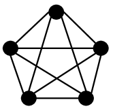
(a) Complete

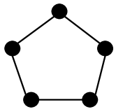
(b) Ring

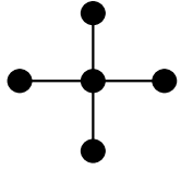
(c) Tree

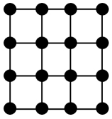
(d) Grid

Figure 1: Interference graph topologies

Varying traffic loads. The graphs in Fig. 2 show the normalized Bethe error on three topologies: complete, ring, and grid. The normalized Bethe errors grow up to at most 0.2, which means that the Bethe error is within 20% of the corresponding target service rate. In addition, for all three topologies, the Bethe error increases as the traffic load increases. Although BAS experiences more errors with higher transmission intensity, it is noteworthy that the mixing time also increases with higher transmission intensity. Thus, the MCMC based algorithms need far more convergence time with the higher transmission intensity although they can get the accurate service rate estimation.

Impact of topology. Bethe error should strongly depend on the underlying topology. As stated in Section III, tree topologies do not have error, while other types of topologies have positive Bethe error. Trees are the ones that are connected and have no cycle. In general, cycles are the major reasons for large Bethe errors, where errors tend to grow with the increasing number of cycles in the topology. In this context, we observe that for complete graphs, the error becomes more significant as the number of links increases, mainly because the number of cycles also increases with the number of links. For ring graphs, we also see the effect of the size of cycle. In Fig. 2(b), the error of 12-links is smaller than that of others, because the cycle becomes similar with a line topology as the number of links increases.

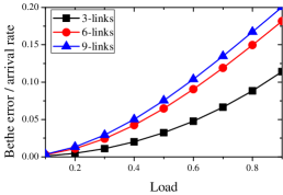
(a) Complete

(b) Ring

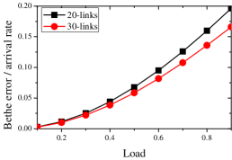
(c) Random

Figure 2: Bethe error for various graphs (where ‘Load’ means arrival rate / capacity when arrival rates are the same)

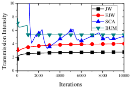
(a) Tree (Star)

(b) Complete

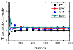
(c) Grid

Figure 3: Trace of transmission intensity

V-B Utility Maximization

Convergence speed. Fig 3 shows the transmission intensity where the graph structure is tree. Note that in tree graphs, all of the algorithms have to converge to the same point, because $e_{B}({\bm{y}})=0$ for all ${\bm{y}}$ when the graph is tree. In the results, BUM becomes stable within only 1000 iterations, whereas the other algorithms does not converge until 10000 iterations. Although the lines of JW and EJW seems to be converged, they grow up very slowly. For the other interference graphs, the trace patterns look similar with the trace of tree graph. All of the algorithms do not converge until 10000 iterations except BUM which converges within 1000 iterations for all graphs. In this simulation, we assume that each update of BUM spends a time slot for one packet transmission. Indeed, since each node $i$ broadcasts just $y_{i}(t)$ at each update, BUM does not need the entire time slot. Thus, we can use BUM as an offline algorithm to find the initial transmission intensities so that the network utility becomes very close to the maximum network utility at the beginning.

Network utility. As we stated in Theorem IV.2, BUM generates error due to the Bethe approximation on intensity update. However, the error is not significant in our test scenarios. By numerical analysis, we get the network utility when BUM is used:-19.9 (for a $5\times 5$ grid interference graph) and -8.1 (for a complete interference graph links). The utility is close to that from the conventional algorithms based on MCMC: -20.6 (for a $5\times 5$ grid interference graph) and -8.05 (for a complete interference graph with 5 links). For the star graph with 5 links, all of the algorithms converge to -3.3. We found that all of the algorithms achieve similar utilities, while BUM converges much faster than prior algorithms.

VI Conclusions

Recently, throughput and utility optimal CSMA algorithms are proposed. The simple and distributed MAC protocol can achieve the both throughput and utility optimal with just locally controlling of parameters. In the previous algorithms, links iteratively update their parameters by their own empirical service and arrival rates. However, their convergence speed is often slow because of the stochastic behavior of scheduling. In this paper, we firstly connect Bethe Free Energy (BFE) with CSMA so as to dramatically reduce the convergence speed. The motivation of this work is that the estimation on the service can be replaced by finding maximum point of the Bethe free energy function since the maximum point gives a good estimation on the service rate. From this motivation, we propose an algorithm by which the CSMA parameters can be nearly optimal without the investigation on service rate when links know the arrival rate of neighbor links by message exchange. In view of network utility, we propose an utility-maximizing algorithm BUM based on the intensity update algorithm using BFE. Since the algorithm does not use empirical values, BUM provably converges in polynomial time, where such a guarantee cannot be achievable via prior known schemes.

-A Notations

Table I contains notations used in this paper.

TABLE I: Notations

Network model
$V$	the set of vertices (nodes)
$n$	the number of vertices (nodes)
$E$	the set of edges such that $(i,j)\in E$ if their transmissions interfere with each other
$G=(V,E)$	the interference graph
$\mathcal{N}(i)$	$\{j:(i,j)\in E\}$, the set of the neighboring links of link $i$
$\bm{\sigma}(t)$	$[\sigma_{i}(t)\in\{0,1\}:i\in V]$, the scheduling vector at time $t$
$\mathcal{I}(G)$	$\{\bm{\sigma}\in\{0,1\}^{n}:\sigma_{i}+\sigma_{j}\leq 1,\forall(i,j)\in E\}$, the set of all feasible schedule vectors
$C(G)$	$\left\{\sum_{\bm{\sigma}\in\mathcal{I}(G)}\alpha_{\bm{\sigma}}\bm{\sigma}:\sum_{\bm{\sigma}\in\mathcal{I}(G)}\alpha_{\bm{\sigma}}=1,~{}\alpha_{\bm{\sigma}}\geq 0,~{}\forall\bm{\sigma}\in\mathcal{I}(G)\right\}$, the set of all possible service rate vectors
${\bm{r}}$	$[r_{i}:i\in V]$, the transmission intensity vector
$s_{i}({\bm{r}})$	the service rate of link $i$ under CSMA with transmission intensity vector ${\bm{r}}$
$\lambda_{i}$	the packet arrival rate at link $i$
Free energies
$F_{G}(\cdot;{\bm{r}})$, $H_{G}(\cdot)$	Gibbs free energy function with intensity vector ${\bm{r}}$ and Gibbs entropy (they are functions of probability distributions on space $\mathcal{I}(G)$)
$F_{B}(\cdot;{\bm{r}})$, $H_{B}(~{}\cdot~{})$	Bethe free energy function with intensity vector ${\bm{r}}$ and Bethe entropy
$D_{B}$	$\{{\bm{y}}:y_{i}\geq 0,y_{i}+y_{j}\leq 1,~{}\mbox{for all}~{}(i,j)\in E\}$, the domain of $F_{B}$ and $H_{B}$
$e_{B}({\bm{r}})$	Bethe error (refer to Definition III.2)
Utilities
$U_{i}(\cdot)$	the utility function of link $i$
$K_{B}({\bm{y}})$, ${\bm{y}}\in D_{B}$	$\beta\cdot\sum_{i\in V}U_{i}(y_{i})+H_{B}({\bm{y}})$, the objective function of BUM

-B Proof of Lemma IV.1

Let $\mathcal{H}({\bm{y}})$ denote the Hessian matrix of $K_{B}({\bm{y}})$ and $\mathcal{H}({\bm{y}})_{ij}$ denote the element of $\mathcal{H}({\bm{y}})$ on $i$-th row and $j$-th column. When the Hessian matrix $\mathcal{H}({\bm{y}})$ is negative definite (${\it i.e.}~{}~{}\bm{x}\cdot\mathcal{H}({\bm{y}})\cdot\bm{x}\leq 0$ for all $\bm{x}$) for all feasible ${\bm{y}},$ $K_{B}({\bm{y}})$ is concave. Therefore, we will show the concaveness of $K_{B}({\bm{y}})$ by showing that $\bm{x}\cdot\mathcal{H}({\bm{y}})\cdot\bm{x}\leq 0$ for all $\bm{x}.$

The diagonal elements $\mathcal{H}({\bm{y}})_{ii}$ are computed as follows:

$$\mathcal{H}({\bm{y}})_{ii}= \beta\cdot U_{i}^{\prime\prime}(y_{i})+(d(i)-1)\frac{1}{1-y_{i}}-\frac{1}{y_{i}}-\sum_{j\in\mathcal{N}(i)}\frac{1}{1-y_{i}-y_{j}}$$

$$= -\alpha\beta\cdot y_{i}^{-\alpha-1}-\frac{1}{y_{i}}-\frac{1}{1-y_{i}}-\sum_{j\in\mathcal{N}(i)}\left(\frac{1}{1-y_{i}-y_{j}}-\frac{1}{1-y_{i}}\right),$$

which is bounded above as follows :

$$\mathcal{H}({\bm{y}})_{ii} <~{}-\sum_{j\in\mathcal{N}(i)}\left(\frac{1}{1-y_{i}-y_{j}}-\frac{1}{1-y_{i}}\right)$$

$$~{}=~{}-\sum_{j\in\mathcal{N}(i)}\left(\frac{y_{j}}{1-y_{i}}\cdot\frac{1}{1-y_{i}-y_{j}}\right),$$

since $-\alpha\beta\cdot y_{i}^{-\alpha-1}-\frac{1}{y_{i}}-\frac{1}{1-y_{i}}<0.$ Moreover, when $y_{i}<1/2,$ we can get more tight bound as follows:

$$\mathcal{H}({\bm{y}})_{ii}< -2d\cdot y_{i}^{-\alpha-1}+(d(i)-1)\frac{1}{1-y_{i}}-\frac{1}{y_{i}}-\sum_{j\in\mathcal{N}(i)}\frac{1}{1-y_{i}-y_{j}}$$

$$\stackrel{{\scriptstyle(a)}}{{<}} -d\cdot y_{i}^{-\alpha-1}-\sum_{j\in\mathcal{N}(i)}\frac{1}{1-y_{i}-y_{j}}$$

$$\stackrel{{\scriptstyle(b)}}{{<}} -\sum_{j\in\mathcal{N}(i)}\left(\frac{1}{y_{i}}+\frac{1}{1-y_{i}-y_{j}}\right)$$

$$= -\sum_{j\in\mathcal{N}(i)}\left(\frac{1-y_{j}}{y_{i}}\cdot\frac{1}{1-y_{i}-y_{j}}\right),$$

where for $(a)$ we use that $y_{i}^{-\alpha-1}>\frac{1}{1-y_{i}}$ when $y_{i}<1/2$ and $(b)$ follows from $y_{i}^{-\alpha-1}>1/y_{i}.$

One can easily compute the non-diagonal elements such that

$$\mathcal{H}({\bm{y}})_{ij}=\mathcal{H}({\bm{y}})_{ji}=\begin{cases}-\frac{1}{1-y_{i}-y_{j}}<0&\mbox{if}~{}~{}(i,j)\in E\cr 0&\mbox{otherwise}.\end{cases}$$

Without loss of generality, let $y_{u}\leq y_{v}$ when the edge is denoted by $(u,v).$ Then,

$$\bm{x}^{T}\mathcal{H}({\bm{y}})\bm{x}=\sum_{i\in V}x_{i}^{2}\mathcal{H}({\bm{y}})_{ii}+\sum_{(i,j)\in E}2x_{i}x_{j}\mathcal{H}({\bm{y}})_{ij}$$

$$<-\sum_{i\in V:y_{i}<\frac{1}{2}}\sum_{j\in\mathcal{N}(i)}\frac{1-y_{j}}{y_{i}}\frac{x_{i}^{2}}{1-y_{i}-y_{j}}-\sum_{i\in V:y_{i}\geq\frac{1}{2}}\sum_{j\in\mathcal{N}(i)}\frac{y_{j}}{1-y_{i}}\frac{x_{i}^{2}}{1-y_{i}-y_{j}}-\sum_{(i,j)\in E}\frac{2x_{i}x_{j}}{1-y_{i}-y_{j}}$$

$$<-\sum_{i\in V}\sum_{j\in\mathcal{N}(i):y_{i}\leq y_{j}}\frac{1-y_{j}}{y_{i}}\frac{x_{i}^{2}}{1-y_{i}-y_{j}}-\sum_{j\in V}\sum_{i\in\mathcal{N}(j):y_{i}<y_{j}}\frac{y_{i}}{1-y_{j}}\frac{x_{j}^{2}}{1-y_{i}-y_{j}}-\sum_{(i,j)\in E}\frac{2x_{i}x_{j}}{1-y_{i}-y_{j}}$$

$$=-\sum_{(i,j)\in E}\Big{(}\frac{1-y_{j}}{y_{i}}\cdot\frac{1}{1-y_{i}-y_{j}}x_{i}^{2}+\frac{2x_{i}x_{j}}{1-y_{i}-y_{j}}+\frac{y_{i}}{1-y_{j}}\cdot\frac{1}{1-y_{i}-y_{j}}x_{j}^{2}\Big{)}$$

$$=-\sum_{(i,j)\in E}\frac{1}{1-y_{i}-y_{j}}\Big{(}\sqrt{\frac{1-y_{j}}{y_{i}}}x_{i}+\sqrt{\frac{y_{i}}{1-y_{j}}}x_{j}\Big{)}^{2}~{}\leq~{}0.$$

Therefore, $\mathcal{H}$ is negative definite matrix.

-C Proof of Lemma IV.2

Recall that

$$\delta_{2} :=\min\left\{c_{2}(t_{*}),\frac{1}{2(\exp(\beta 2^{\alpha})+1)}\right\},\quad\quad\delta_{1}:=\min\left\{c_{1}(t_{*}),\frac{\beta 2^{\alpha}\delta_{2}^{d}}{4(1+\beta 2^{\alpha}d\delta_{2}^{d-1})}\right\},$$

$$\delta_{3} :=\min\left\{c_{2}(t_{*}),\frac{\delta_{1}}{2\exp(\beta\delta_{1}^{-\alpha})}\right\},~{}\mbox{and}~{}$$

$$t_{*} :=\inf\left\{\tau:\frac{1}{\sqrt{t}}\left|\frac{\partial K_{B}({\bm{y}}(t))}{\partial y_{i}}\right|<\frac{1}{2}\min\{c_{1}(t),c_{2}(t)\}~{}~{}\forall~{}t\geq\tau\right\}.$$

In this proof, for notational simplicity, we introduce $\varepsilon_{1}:=\frac{\beta 2^{\alpha}\delta_{2}^{d}}{4(1+\beta 2^{\alpha}d\delta_{2}^{d-1})}$, $\varepsilon_{2}:=\frac{1}{2(\exp(\beta 2^{\alpha})+1)}$, and $\varepsilon_{3}:=\frac{\delta_{1}}{2\exp(\beta\delta_{1}^{-\alpha})}$.

We start by stating three key lemmas which play key roles in the proof of Lemma IV.2. First, by Lemma .1, the gradient of $K_{B}({\bm{y}}(t))$ is bounded above with $\frac{1}{2}\min\{c_{1}(t),c_{2}(t)\}$ after time $t^{*}.$ Next, we show that ${\bm{y}}(t+1)$ goes away from the boundary of $D^{*}_{B}$ when ${\bm{y}}(t)$ is within $2\min\{c_{1}(t),c_{2}(t)\}$ away from the boundary, by Lemma .2, Lemma .3, and Lemma .4. Then, the update of ${\bm{y}}(t)$ does not hit the boundary of $D^{*}_{B}$ always.

Lemma .1

There exists $t_{*}$ such that , for every link $i$

$$\frac{1}{\sqrt{t}}\left|\frac{\partial K_{B}({\bm{y}}(t))}{\partial y_{i}}\right|<\frac{1}{2}\min\{c_{1}(t),c_{2}(t)\},~{}~{}\forall~{}t\geq t_{*}.$$

Proof:

To conclude this proof, we will show that

$$\lim_{t\rightarrow\infty}\frac{1}{\min\{c_{1}(t),c_{2}(t)\}\sqrt{t}}\frac{\partial K_{B}({\bm{y}}(t))}{\partial y_{i}}=0.$$

The proof starts from the range of first derivative function at time $t$:

$$\frac{\partial K_{B}({\bm{y}}(t))}{\partial y_{i}}= U^{\prime}_{i}(y_{i}(t))-(d(i)-1)\log(1-y_{i}(t))-\log y_{i}(t)+\sum_{j\in\mathcal{N}(i)}\log(1-y_{i}(t)-y_{j}(t))$$

$$\leq \beta y_{i}(t)^{-\alpha}-\log\frac{y_{i}(t)}{1-y_{i}(t)}+\sum_{j\in\mathcal{N}(i)}\log\frac{1-y_{i}(t)-y_{j}(t)}{1-y_{i}(t)}$$

$$\leq \beta y_{i}(t)^{-\alpha}-\log\frac{y_{i}(t)}{1-y_{i}(t)}$$

$$\leq \big{(}c_{1}(t)\big{)}^{-\alpha}-\log(c_{1}(t)),$$

where the last inequality stems from the fact that $y_{i}(t)\geq c_{1}(t).$ Therefore, from (13),

$$\lim_{t\rightarrow\infty}\frac{1}{\sqrt{t}}\frac{1}{\min\{c_{1}(t),c_{2}(t)\}}\frac{\partial K_{B}({\bm{y}}(t))}{\partial y_{i}}\leq 0.$$

Now, the remaining part is $\lim_{t\rightarrow\infty}\frac{1}{\min\{c_{1}(t),c_{2}(t)\}\sqrt{t}}\frac{\partial K_{B}({\bm{y}}(t))}{\partial y_{i}}\geq 0.$ Since $1-y_{i}(t)-y_{j}(t)\geq c_{2}(t)$ for all $i\neq j$,

$$\frac{\partial K_{B}({\bm{y}}(t))}{\partial y_{i}} =U^{\prime}_{i}(y_{i}(t))-(d(i)-1)\log(1-y_{i}(t))-\log y_{i}(t)+\sum_{j\in\mathcal{N}(i)}\log(1-y_{i}(t)-y_{j}(t))$$

$$\geq\sum_{j\in\mathcal{N}(i)}\log(1-y_{i}(t)-y_{j}(t))\geq d(i)\log(c_{2}(t)).$$

Therefore, from (13),

$$\lim_{t\rightarrow\infty}\frac{1}{\min\{c_{1}(t),c_{2}(t)\}\sqrt{t}}\frac{\partial K_{B}({\bm{y}}(t))}{\partial y_{i}}\geq 0.$$

∎

Lemma .2

If $y_{i}\geq 1-2\varepsilon_{2}$ and ${\bm{y}}\in D^{*}_{B}$, $\frac{\partial K_{B}({\bm{y}})}{\partial y_{i}}<0$.

Proof:

$$\frac{\partial K_{B}({\bm{y}})}{\partial y_{i}} =\beta y_{i}^{-\alpha}-(d(i)-1)\log(1-y_{i})-\log y_{i}+\sum_{j\in\mathcal{N}(i)}\log(1-y_{i}-y_{j})$$

$$=\beta y_{i}^{-\alpha}-\log\frac{y_{i}}{1-y_{i}}+\sum_{j\in\mathcal{N}(i)}\log\frac{1-y_{i}-y_{j}}{1-y_{i}}$$

$$<\beta y_{i}^{-\alpha}-\log\frac{y_{i}}{1-y_{i}}$$

$$\leq\beta(\frac{1}{2})^{-\alpha}-\log\frac{1-2\varepsilon_{2}}{2\varepsilon_{2}}\leq 0,$$

where the last inequality is from our choice of

$$\varepsilon_{2}=\frac{1}{2(\exp(\beta 2^{\alpha})+1)}.$$

∎

Lemma .3

If $y_{i}\leq 2\varepsilon_{1}$ and ${\bm{y}}\in D^{*}_{B}$, $\frac{\partial K_{B}({\bm{y}})}{\partial y_{i}}>0$.

Proof:

$$\frac{\partial K_{B}({\bm{y}})}{\partial y_{i}} =\beta y_{i}^{-\alpha}-(d(i)-1)\log(1-y_{i})-\log y_{i}+\sum_{j\in\mathcal{N}(i)}\log(1-y_{i}-y_{j})$$

$$>\beta y_{i}^{-\alpha}-\log y_{i}+d\,\log\left(\delta_{2}-y_{i}\right)$$

$$=\log\frac{\exp(\beta y_{i}^{-\alpha})\left(\delta_{2}-y_{i}\right)^{d}}{y_{i}}$$

$$=\log\frac{\exp(\beta y_{i}^{-\alpha})\delta_{2}^{d}\left(1-\frac{y_{i}}{\delta_{2}}\right)^{d}}{y_{i}}\geq 0,$$

where the last inequality stems from the fact that $y_{i}\leq 2\varepsilon_{1}$ with our choice of $\varepsilon_{1}=\frac{\beta 2^{\alpha}\delta_{2}^{d}}{4(1+\beta 2^{\alpha}d\delta_{2}^{d-1})}$ as

$$\frac{\beta y_{i}^{-\alpha}\delta_{2}^{d}\left(1-\frac{y_{i}}{\delta_{2}}\right)^{d}}{y_{i}}\geq\frac{\beta y_{i}^{-\alpha}\delta_{2}^{d}\left(1-d\frac{y_{i}}{\delta_{2}}\right)}{y_{i}}\geq\frac{\beta 2^{\alpha}\delta_{2}^{d}\left(1-d\frac{y_{i}}{\delta_{2}}\right)}{y_{i}}\geq 1$$

and $\exp(\beta y_{i}^{-\alpha})\geq\beta y_{i}^{-\alpha}$ since $\beta y_{i}^{-\alpha}\geq 1$. ∎

Lemma .4

If $y_{i}+y_{j}\geq 1-2\varepsilon_{3}$ and ${\bm{y}}\in D^{*}_{B}$, $\frac{\partial K_{B}({\bm{y}})}{\partial y_{i}}<0$.

Proof:

$$\frac{\partial K_{B}({\bm{y}})}{\partial y_{i}} =\beta y_{i}^{-\alpha}-(d(i)-1)\log(1-y_{i})-\log y_{i}+\sum_{k\in\mathcal{N}(i)}\log(1-y_{k}-y_{i})$$

$$=\beta y_{i}^{-\alpha}-\log{y_{i}}+\log(1-y_{i}-y_{j})+\sum_{k\in\mathcal{N}(i)\setminus j}\log\frac{1-y_{k}-y_{i}}{1-y_{i}}$$

$$<\beta y_{i}^{-\alpha}-\log{y_{i}}+\log(1-y_{i}-y_{j})$$

$$\leq\beta y_{i}^{-\alpha}-\log\delta_{1}+\log 2\varepsilon_{3}\leq 0,$$

where the last inequality is from our choice of $\varepsilon_{3}=\frac{\delta_{1}}{2\exp(\beta\delta_{1}^{-\alpha})}.$ ∎

Completing the proof of Lemma IV.2. For proving ${\bm{y}}(t)\in D^{*}_{B}$, we need the following three inequalities:

$$y_{i}(t) < 1-\delta_{2}$$ (17)

$$y_{i}(t) > \delta_{1}$$ (18)

$$y_{i}(t)+y_{j}(t) < 1-\delta_{3}.$$ (19)

Proof of (17). Let $t_{2}:=c_{2}^{-1}(\delta_{2}).$ Then, for time $t<t_{2},$ $y_{i}(t)<1-\delta_{2}$ from the dynamic bound. For time $t\geq t_{2},$ $y_{i}(t)<1-\delta_{2},$ since $\frac{1}{\sqrt{t}}\left|\frac{\partial K_{B}({\bm{y}})}{\partial y_{i}}\right|<\frac{c_{2}(t)}{2}\leq\frac{\delta_{2}}{2}$ from Lemma .1 and $\frac{\partial K_{B}({\bm{y}})}{\partial y_{i}}<0$ if $y_{i}>1-2\delta_{2},$ from Lemma .2.

Proof of (18). Similarly, let $t_{1}:=c_{1}^{-1}(\delta_{1}).$ Then, for time $t<t_{1},$ $y_{i}(t)>\delta_{1}$ from the dynamic bound. For time $t\geq t_{1},$ $y_{i}(t)>\delta_{1},$ since $\frac{1}{\sqrt{t}}\left|\frac{\partial K_{B}({\bm{y}})}{\partial y_{i}}\right|<\frac{c_{1}(t)}{2}<\frac{\delta_{1}}{2}$ from Lemma .1 and $\frac{\partial K_{B}({\bm{y}})}{\partial y_{i}}>0$ if $y_{i}<2\delta_{1},$ from Lemma .3.

Proof of (19). Let $t_{3}:=c_{2}^{-1}(\delta_{3}).$ Then, for time $t<t_{3},$ $y_{i}(t)+y_{j}(t)<1-\delta_{3}$ from the dynamic bound. For time $t\geq t_{3},$ $y_{i}(t)+y_{j}(t)<1-\delta_{3},$ since $\frac{1}{\sqrt{t}}\left(\left|\frac{\partial K_{B}({\bm{y}})}{\partial y_{i}}\right|+\left|\frac{\partial K_{B}({\bm{y}})}{\partial y_{j}}\right|\right)<c_{2}(t)\leq\delta_{3}$ from Lemma .1 and $\max\{\frac{\partial K_{B}({\bm{y}})}{\partial y_{i}},\frac{\partial K_{B}({\bm{y}})}{\partial y_{i}}\}<0$ if $y_{i}+y_{j}>1-2\delta_{3},$ from Lemma .4.

By combining (17), (18) and (19), it follows that ${\bm{y}}(t)\in D^{*}_{B}$ for all $t.$

References

• [1] J. S. Yedidia, W. T. Freeman, and Y. Weiss, “Constructing free energy approximations and generalized belief propagation algorithms,” IEEE Transactions on Information Theory, vol. 51, pp. 2282–2312, 2005.
• [2] L. Jiang, D. Shah, J. Shin, and J. Walrand, “Distributed random access algorithm: Scheduling and congestion control,” IEEE Transactions on Information Theory, vol. 56, no. 12, pp. 6182 –6207, dec. 2010.
• [3] L. Jiang and J. Walrand, “A distributed CSMA algorithm for throughput and utility maximization in wireless networks,” IEEE/ACM Transactions on Networking, vol. 18, no. 3, pp. 960 –972, June 2010.
• [4] J. Liu, Y. Yi, A. Proutiere, M. Chiang, and H. V. Poor, “Towards utility-optimal random access without message passing,” Wiley Journal of Wireless Communications and Mobile Computing, vol. 10, no. 1, pp. 115–128, Jan. 2010.
• [5] N. Hegde and A. Proutiere, “Simulation-based optimization algorithms with applications to dynamic spectrum access,” in Proceedings of CISS, 2012.
• [6] L. Tassiulas and A. Ephremides, “Stability properties of constrained queueing systems and scheduling for maximum throughput in multihop radio networks,” IEEE Transactions on Automatic Control, vol. 37, no. 12, pp. 1936–1949, December 1992.
• [7] X. Lin, N. B. Shroff, and R. Srikant, “A tutorial on cross-layer design in wireless networks,” IEEE Journal on Selected Areas in Communications, vol. 24, pp. 1452–1463, 2006.
• [8] Y. Yi and M. Chiang, “Stochastic network utility maximisation: a tribute to Kelly’s paper published in this journal a decade ago,” European Transactions on Telecommunications, vol. 19, no. 4, pp. 421–442, 2008.
• [9] S.-Y. Yun, Y. Yi, J. Shin, and D. Y. Eun, “Optimal CSMA: a survey,” in Proceedings of ICCS, 2012.
• [10] L. Jiang, M. Leconte, J. Ni, R. Srikant, and J. Walrand, “Fast mixing of parallel Glauber dynamics and low-delay CSMA scheduling,” in Proceedings of infocom, april 2011, pp. 371 –375.
• [11] R. Kindermann, J. Snell, and A. M. Society, Markov random fields and their applications, ser. Contemporary mathematics.   American Mathematical Society, 1980. [Online]. Available: http://books.google.com/books?id=NeVQAAAAMAAJ
• [12] J. G. David Forney, “Codes on graphs: News and views,” in Conference on Information Sciences and Systems, 2001.
• [13] Y. W. K. P. Murphy and M. Jordan, “Loopy belief propagation for approximate inference: an empirical study,” in In Proceedings of Uncertainty in Artificial Intelligence, 1999.
• [14] J. Mo and J. Walrand, “Fair end-to-end window-based congestion control,” IEEE/ACM Transactions on Networking, vol. 8, no. 5, pp. 556–567, 2000.
• [15] C. H. Kai and S. C. Liew, “Applications of belief propagation in CSMA wireless networks,” IEEE/ACM Transactions on Networking, vol. 20, no. 4, pp. 1276–1289, 2012.
• [16] P. Djukic, “Scheduling algorithms for TDMA wireless multihop networks,” Ph.D. dissertation, University of Toronto, 2008.
• [17] Y. Yi, G. de Veciana, and S. Shakkottai, “Learning contention patterns and adapting to load/topology changes in in a MAC scheduling algorithm,” in Proceedings of IEEE WiMesh, 2006.
• [18] H. Georgii, Gibbs Measures and Phase Transitions, ser. De Gruyter Studies in Mathematics.   W. de Gruyter, 1988, no. V. 9. [Online]. Available: http://books.google.com/books?id=3YdI0yww12QC
• [19] V. Chandrasekaran, M. Chertkov, D. Gamarnik, D. Shah, and J. Shin, “Counting independent sets using the bethe approximation,” SIAM Journal on Discrete Mathematics, vol. 25, no. 2, pp. 1012–1034, 2011.