Effective model for electronic properties of the quasi one-dimensional purple bronze Li_0.9Mo₆O₁₇ based on ab-initio calculations

Abstract

We investigate the electronic structure of the strongly anisotropic, quasi low dimensional purple bronze Li_0.9Mo₆O₁₇. Building on all-electron ab-initio band structure calculations we obtain an effective model in terms of four maximally localized Wannier orbitals, which turn out to be far from atomic like. We find two half-filled orbitals arranged in chains running along one crystallographic direction, and two full orbitals in perpendicular directions, respectively. The possibility to reduce this model to only two orbitals forming two chains per unit cell with inter-chain coupling is discussed. Transport properties of these models show high anisotropy, reproducing trends of the experimentally determined values for the dc conductivity. We also consider basic effects of electron-electron interactions using the (extended) Variational Cluster Approach and Dynamical Mean Field Theory. We find good agreement with experimental photo emission data upon adding moderate on-site interaction of the order of the band width to the ab-initio derived tight-binding Hamiltonian. The obtained models provide a profound basis for further investigations on low-energy Luttinger liquid properties or to study electronic correlations within computational many-body theory.

I Introduction

The electronic structure of highly anisotropic materials shows a plethora of interesting effects. Quantum many-body dynamics in quasi low dimensional systems becomes important and dominant in many regions of their rich phase diagram. This often implies unconventional ground states, such as non-Fermi-liquid or Luttinger-liquid states. One prominent example for this class of materials is the lithium molybdenum purple bronze Li_0.9Mo₆O₁₇, McCarroll and Greenblatt (1984) a molybdenum oxide bronze with quasi one-dimensional properties. Greenblatt (1988)

Experimental structure analysis using X-rays Onoda et al. (1987) as well as neutrons da Luz et al. (2011) determined a monoclinic crystal structure. The conduction electrons are mostly located on two molybdenum octahedral sites which are arranged in double zig-zag chains along the $b$ axis. This leads to a very high anisotropy of the material, which has been studied by several techniques using resistivity measurements, Greenblatt et al. (1984); da Luz et al. (2007); Mercure et al. (2012a); Xu et al. (2009); dos Santos et al. (2008); Matsuda et al. (1986a) conductivity under pressure, Filippini et al. (1989) magneto resistance, Xu et al. (2009); Chen et al. (2010) thermal expansion, dos Santos et al. (2007) optical conductivity, Choi et al. (2004); Degiorgi et al. (1988) the Nernst effect, Cohn et al. (2012a) thermal conductivity,Wakeham et al. (2011) thermopower Boujida et al. (1988) and muon spectroscopy. Chakhalian et al. (2005)

The electronic properties have been addressed using angle-resolved photo emission spectroscopy (ARPES) Denlinger et al. (1999); Wang et al. (2006, 2009); Gweon et al. (2003, 2004); Wang et al. (2008); Dudy et al. (2013); Gweon et al. (2002, 2000) and scanning tunneling microscopy (STM), Hager et al. (2005); Podlich et al. (2013) which argued for one-dimensional Luttinger liquid physics. Giamarchi (2004); Pustilnik et al. (2006); Khodas et al. (2007); Meden and Schönhammer (1992); Voit (1993); León et al. (2007); Gweon et al. (2000) Other studies disputed this claim. Xue et al. (1999) The evolution and the current status of work in that direction is summed up in a recent review article. Dudy et al. (2013) A temperature dependent dimensional crossover Biermann et al. (2001); Berthod et al. (2006); Raczkowski and Assaad (2012) which induces coherence for the perpendicular electron motion, has been studied using neutron diffraction. da Luz et al. (2011)

Apart from intriguing physical effects of effective low dimensionality the material shows superconductivity below $1.9$ K Schlenker et al. (1985); Greenblatt (1988); Matsuda et al. (1986b); Ekino et al. (1987); Mercure et al. (2012b) and a metal-insulator transition is observed at around $24$ K. Schlenker et al. (1985); Greenblatt et al. (1984); Sato et al. (1987); Choi et al. (2004) No evidence for a Peierls instability has been reported, Gweon et al. (2001) and a possible charge density wave (CDW) phase is still under debate. Dumas and Schlenker (1993); Chudzinski et al. (2012); Merino and McKenzie (2012); Hager et al. (2005) Recent studies have argued for a compensated metal. Cohn et al. (2012b) All data are summed up in a conjectured electronic phase diagram as presented in Ref. Merino and McKenzie, 2012.

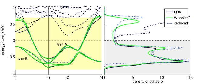
Figure 1: (Color online) Left: LDA band structure (solid black) in the vicinity of the Fermi energy $\epsilon_{F}$ plotted along a two-dimensional path in the reciprocal $b$-$c$ plane. The four bands of the full Wannier projected Hamiltonian are shown on top (solid green) next to the data for the reduced model (dash-dotted blue). Right: DOS of the LDA calculation (black), the full Wannier model (solid green) and the reduced model (dash-dotted blue).

Theoretical ab-initio studies of the electronic structure using a tight-binding method, Whangbo and Canadell (1988) as well as a linearized muffin-tin orbital (LMTO) Popović and Satpathy (2006); Jarlborg et al. (2012) calculation in the local density approximation (LDA) have been conducted. These approaches were successful in providing a broad picture of the ”high energy” physics of Li_0.9Mo₆O₁₇, accounting for the high anisotropy. Although experiments testified a wealth of remarkable low-energy properties and different quantum ground states, more detailed theoretical investigations, including interactions and low dimensionality, emerged in recent years only.

Chudzinski et al. Chudzinski et al. (2012) investigated the quasi one-dimensionality and have been able to extract an effective low-energy theory within the Tomonaga-Luttinger-liquid framework. Their approach is based on an atomic orbital tight-binding model with parameters such that it matches an LDA LMTO band-structure calculation. Motivated by the crystal structure of Li_0.9Mo₆O₁₇ the model was set up with four molybdenum $d$ orbitals in a zig-zag ladder arrangement including on-site as well as non-local electronic interactions. It was found that within this model Luttinger-liquid low-energy parameters can be obtained, which are consistent with experimental findings.

Another recent work Merino and McKenzie (2012) proposes a two-dimensional model from Slater-Koster Slater and Koster (1954) atomic orbitals also including non-local electronic interactions. Again an Ansatz with four Mo orbitals in zig-zag ladder arrangement was applied. The authors argue, based on electron counting, that there are two electrons to be shared among the four equivalent Mo atoms, leading to quarter-filled orbitals. The bandwidth obtained with this Ansatz for the two bands crossing the Fermi level is in rough agreement with Density Functional Theory (DFT) calculations. Details of the band structure such as curvatures, however, and also the bands just below the Fermi level which are of similar Mo $d$ character, cannot be reproduced by this Slater-Koster model.

The main purpose of this work is to establish an unbiased, general purpose tight-binding model for the electronic properties of Li_0.9Mo₆O₁₇ based on ab-initio calculations. Such a model is intended to serve as a basis to study the role of electronic correlations by adding interactions, be it in a computational many-body theory or in a one-dimensional renormalization group (RG) framework. In contrast to previous work Merino and McKenzie (2012) we propose a model based on maximally-localized Wannier orbitals Marzari et al. (2012, 2003) instead of linear combination of atomic orbitals. Four molecular-like orbitals are obtained in a fully ab-initio approach from an all-electron DFT calculation. Our results unambiguously show that, using a set of four Wannier orbitals in the unit cell, the model consists of two half-filled as well as two filled orbitals. As we will show below, the DFT band structure is perfectly reproduced in this basis set of Wannier functions.

This model describes the momentum resolved electronic structure as observed in ARPES Wang et al. (2009) experiments and reproduces highly anisotropic transport characteristics. Greenblatt et al. (1984); Chen et al. (2010); Choi et al. (2004); da Luz et al. (2007); Mercure et al. (2012a); Xu et al. (2009); Wakeham et al. (2011) Furthermore we discuss an even simpler two-orbital effective model which can be derived from the four-orbital model.

In the second part of the paper we conduct a first (qualitative) study of effects of interactions on the electron dynamics within this effective Wannier model. Even more so due to the low dimensionality the interacting model is in general difficult to approach. By applying RG as well as density matrix renormalization group (DMRG) Schollwöck (2011) in certain limits (chains, ladders) their essential physics can be understood. Merino and McKenzie (2012) To solve the full low dimensional interacting Hubbard-type model, general frameworks as for example (cluster) dynamical mean field theory ((C)DMFT)-like approaches Maier et al. (2005) have been applied, where the self-energy of the system is restricted to a finite length scale.

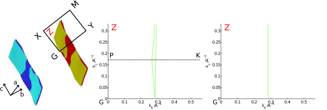
Figure 2: (Color online) Calculated Fermi surface. Left: The ab-initio result (image created using XCrySDen Kokalj (2003)). Center: In-plane projection of the result for the four-orbital Wannier model. Right: In-plane projection of the result for the reduced model, where type (A) orbitals are strictly one-dimensional and the two Fermi sheets are degenerate.

Realistic modeling is a relatively new and rapidly developing field. Solovyev (2008); Imada and Miyake (2010); Held et al. (2001) In this work we study (simple) electron-electron interactions in the effective model using complementary numerical techniques. First, we use cluster perturbation theory (CPT) Gros and Valenti (1993); Sénéchal et al. (2000) as well as the (extended) Aichhorn et al. (2004, 2005) Variational Cluster Approach Potthoff et al. (2003) ((e)VCA) in the spirit of LDA+VCA. Chioncel et al. (2007); Aichhorn et al. (2009) The choice of these methods is motivated by the expected reduced effective dimensionality of the material which renders the non-local character of the VCA self-energy an interesting perspective. Second, we apply the well-established LDA+DMFT Anisimov et al. (1997); Katsnelson and Lichtenstein (1999); Chioncel et al. (2003) approach, which neglects non-local correlations, but on the other hand performs superior in describing the quasi-particle features at low energy as compared to VCA. For all applied methods we find that a moderate value of on-site interactions strength is capable of describing the electron dynamics best and in good agreement with ARPES experiments. We discuss the influence of a hybridization mechanism of the two bands right at the Fermi energy with the two bands slightly below, not accounted for in previous work.

This paper is organized as follows: in Sec. II we report accurate all electron DFT data from which we obtain a model in terms of maximally-localized Wannier functions. A further simplified model for Li_0.9Mo₆O₁₇ with reduced number of hopping parameters is discussed in Sec. II.3. We present results for the anisotropic conductivity in Sec. III and compare to transport measurements. The electron dynamics of the interacting effective model are presented and compared to ARPES experiments in Sec. IV before concluding in Sec. V.

II From crystal structure to an effective electronic model

II.1 Ab-initio electronic structure

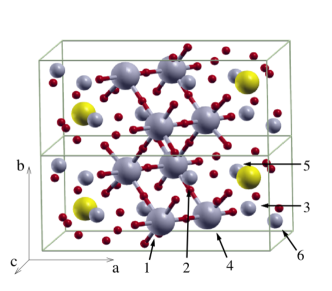
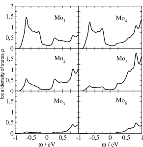
Figure 3: Top plot: Crystal structure. In $a$ and $c$ direction one unit cell, and in $b$ direction 2 unit cells are shown. Big gray balls are Mo₁/Mo${}_{1}^{\prime}$ and Mo₄/Mo${}_{4}^{\prime}$ atoms, showing the zig-zag chain structure along $b$. Small gray: other Mo sites. The numbers next to the black arrows denote the atom number. Small red balls are oxygen, and the yellow balls Li atoms. This image has been created using XCrySDen. Kokalj (2003) Bottom plot: Partial DOS of the six in-equivalent Mo atoms in the unit cell. Top row: atoms Mo₁ and Mo₄, forming the zig-zag chains. Middle row: Mo₂ and Mo₅. Bottom row: Mo₃ and Mo₆.

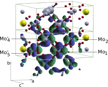
Figure 4: Visualization of one type (A) Wannier orbital. Similar as in Fig. 3, two unit cells in $b$ direction are shown, the Wannier function is centered in the lower unit cell. The center of the Wannier function is located in between atoms Mo₁ and Mo${}_{4}^{\prime}$. Arrows mark the atoms with significant contribution to the Wannier function: in-chain atoms Mo₁ and Mo${}_{4}^{\prime}$, and adjacent atoms Mo₂ and Mo${}_{5}^{\prime}$. Color coding as in the top panel of Fig. 3. For the Wannier functions, blue and green lobes denote positive and negative phase, resp. The image has been created using XCrySDen. Kokalj (2003)

We obtain the electronic structure for ideal Li₁Mo₆O₁₇ from a non-spin-polarized, full-potential linearized augmented plane wave (FP-LAPW) Slater (1937); Andersen (1975); Singh (1991); Sjöstedt et al. (2000) DFT Hohenberg and Kohn (1964); Kohn and Sham (1965) calculation as implemented in the WIEN2k package. Blaha et al. (2001) The unit-cell parameters and crystal structure are taken from X-ray data,Onoda et al. (1987) which have been recently confirmed by neutron diffraction experiments. da Luz et al. (2011) The space group is monoclinic (prismatic) $P2_{1}/m$ with lattice parameters $a=12.762(2)$ Å, $b=5.523(1)$ Å, $c=9.499(1)$ Å, $\beta=90.61(1)^{\circ}$ and $Z=2$, leading to a $48$-atom unit cell [Li₁Mo₆O₁₇]₂. foo (a)

All results presented in this work are calculated with the exchange-correlation potential treated in the LDA. Ceperley and Alder (1980) We checked that the generalized-gradient approximation (GGA - PBE Perdew et al. (1996)) gives indistinguishable results for the band structures. Our results are converged in terms of the size of the FP-LAPW basis set, which is determined by the $RK_{\text{max}}$ parameter in WIEN2k. By performing calculations for different $RK_{\text{max}}$ we found that $RK_{\text{max}}=7.0$ and $RK_{\text{max}}=6.0$ gave the same results, with band energies within $10^{-3}\,$eV, only at $RK_{\text{max}}=5.0$ deviations become visible. Therefore, also due to the computational complexity of the problem, all results presented here are obtained with a $RK_{\text{max}}=6.0$ basis set.

The obtained electronic structure $\mathbf{\epsilon}_{\text{KS}}(\mathbf{k})$ is visualized along the standard path of the $b$-$c$ plane in reciprocal space (Y-G-X-M) (see also Fig. 2) in Fig. 1 (left). In order to compare to ARPES experiment, we modeled lithium-vacant Li_0.9Mo₆O₁₇ by a rigid band shift of $0.03\,$eV of the LDA bands. Popović and Satpathy (2006) We find a combined bandwidth of the four bands in the vicinity of the Fermi energy $\epsilon_{F}$ of $W\approx 1.82$ eV and two Fermi velocities of $v_{F,1}\approx 0.99\cdot 10^{5}\,\frac{\text{m}}{\text{s}}$ and $v_{F,2}\approx 0.93\cdot 10^{5}\,\frac{\text{m}}{\text{s}}$, roughly one order of magnitude lower than in free electron metals. Ashcroft and Mermin (1976) The corresponding electronic density of states (DOS) is shown in Fig. 1 (right). The LDA DOS is obtained by Gaussian integration ($\sigma\approx 0.02$ eV) using the tetrahedron method on a grid of $216$ $k$-points in the irreducible Brillouin zone (BZ).

By and large the electronic structure compares well to previous data reported in early works of Whangbo et al. Whangbo and Canadell (1988) from an empirical tight-binding method, and also to more recent LMTO calculations within the atomic sphere approximation (ASA) from Popovic et al. Popović and Satpathy (2006) But note that in particular the band crossings/hybridizations on the X-M line as well as the lowest empty bands at $\sim 1$ eV above $\epsilon_{F}$ are apparently different. Since we checked accurately the convergence of the all-electron FP-LAPW calculations the difference is most likely to come from the approximations introduced in LMTO-ASA and tight-binding calculations.

The one-dimensionality of the material becomes manifest in the Fermi surface which is shown in Fig. 2 (left). Arising from two bands crossing the Fermi energy, it consists of two sheets warping in $c$ direction, cutting the $b$ axis and being roughly constant in $a$ direction. In experiments Allen (2013) the maximum splitting of the Fermi surface $(<10^{-3}\AA^{-1})$ is observed along the $\overline{\text{PK}}$ line. Our LDA calculations yield the maximum splitting along the very same line, see Fig. 2, but the magnitude is much larger ($\approx 0.021\AA^{-1}$). In previous LDA calculations Popović and Satpathy (2006) an even larger splitting of $\approx 0.045\AA^{-1}$ was found. This discrepancy of the theoretical results with experiment is likely due to the improper treatment of strong non-local electronic correlations in the LDA.

II.2 Realistic effective model

To construct an effective model we have to identify the origin (orbital character and atom) of those electronic states which are most important for the physical properties i.e. those close to the Fermi energy $\epsilon_{F}$. We plot in the bottom panel of Fig. 3 the partial DOS for the six in-equivalent Mo atoms in the unit cell. One can nicely see that Mo₁ and Mo₄ contribute most to the DOS at $\epsilon_{F}$ (for nomenclature see Figure 2 in Onoda et al. Onoda et al. (1987)). In the top panel of Fig. 3 we show the crystal structure, with emphasis on those Mo₁ and Mo₄ (including the equivalent Mo${}_{1}^{\prime}$ and Mo${}_{4}^{\prime}$) atoms. It is evident that these atoms form the two adjacent zig-zag chains running along the $b$-axis, giving rise to the two quasi-one-dimensional bands crossing $\epsilon_{F}$. The atoms Mo₂ and Mo₅ are sitting next to the chains, and thus have some smaller contributions. The other two Mo atoms are far away from the chains, and thus contribute hardly anything to the weight around $\epsilon_{F}$. This analysis of the orbital character shows clearly that the bands around $\epsilon_{F}$ originate mainly from only four atoms (Mo₁, Mo₄, and Mo${}_{1}^{\prime}$, Mo${}_{4}^{\prime}$, respectively) in the unit cell.

To construct an effective model, we take the electronic wave function data $\mathbf{\phi}_{\text{KS}}$ in an energy window of $[-0.9,0.7]$ eV, that comprises the 4 relevant bands as shown in Fig. 1. The lower bound of the energy window for projection is straightforward to choose because the gap between the four considered molybdenum $d$ bands and the next lower bands is larger than $1.5$ eV. The upper bound is more involved since bands with different character penetrate the energy window from above, and are entangled with the two bands crossing the Fermi energy. In order to get a good description of the bands, we had to use the disentanglement procedure of Wannier90 with a frozen energy window of $[-0.9,0.0]$ eV.

We project this data onto four maximally-localized Wannier orbitals Marzari et al. (2012) $\omega_{\alpha}$ using Wannier90 Mostofi et al. (2008) and the Wien2Wannier Kunes et al. (2010) interface. As initial seed, we chose one $d_{xy}$ orbital on each of the Mo₁, Mo₄, Mo${}_{1}^{\prime}$, and Mo${}_{4}^{\prime}$ atoms.

Although starting from a seed with atomic orbitals, the calculated Wannier functions, however, have quite different character. They can be divided into two kinds. Type (A), which is oriented along chains in $b$ direction, and type (B) which is in some sense orthogonal in real space, mediating between the chains in $b$ direction. The orbitals contributing to the states around $\epsilon_{F}$ are of type (A), and one of these orbitals is shown in Fig. 4. One can clearly see the $d_{xy}$ orbital character, forming the zig-zag chains, around atoms Mo₁ and Mo${}_{4}^{\prime}$, where most of the orbital weight is located. In consistency with the partial DOS, Fig. 3, some contribution also comes from atoms Mo₂ and Mo${}_{5}^{\prime}$, since they are adjacent to the chains, as shown in Fig. 4.

The splitting into two types of orbitals can be understood from the band structure. Only two bands cross $\epsilon_{F}$, which results in two equivalent Wannier functions (A). The other two bands, lying below $\epsilon_{F}$ are spanned by another set of two equivalent Wannier functions (B), respecting the crystal symmetry.

We would like to emphasize that these orbitals are far from atomic like. We estimate their spread from the square root of the spread functional of Wannier90, which yields $5.2$ Å for orbital type (A), and $4.4$ Å for orbital type (B). We also want to note that the Wannier functions are not centered on a Mo site. Instead, Fig. 4 clearly shows that the centers are located in the middle of a bond between two Mo sites. For type (A), one orbital has its center between atoms Mo₁ and Mo${}_{4}^{\prime}$, the other between Mo${}_{1}^{\prime}$ and Mo₄, resp. In that sense, these Wannier orbitals can be regarded as bond-centered molecular-like orbitals.

The origin of the large spread in real space is the very limited number of bands that are taken into account in the Wannier construction scheme. Taking all $d$ orbitals of the Mo₁, Mo${}_{1}^{\prime}$, Mo₄, and Mo${}_{4}^{\prime}$ atoms as well as the bridging oxygen $p$-orbitals into account would of course result in much better localization. However, the Hamiltonian then describes many bands, and not only the most important four bands in the vicinity of $\epsilon_{F}$. A similar effect can be observed for instance in the construction of the one-band model in cuprate superconductors. Also there, taking only the $d_{x^{2}-y^{2}}$ orbital into the construction results in quite large Wannier orbitals with long tails. Pavarini et al. (2001)

Concerning the electron charge in the Wannier orbitals we find that orbitals of type (A) are half-filled, whereas orbitals of type (B) are identified as (almost) filled. For lithium-vacant purple bronze, we find a total occupation of $\approx 5.8$ electrons in these four bands, since there are two lithium ions in the unit cell, each contributing $\approx 0.1$ hole doping. In the remainder of the paper, we will therefore use for all discussions an average filling of the four bands of $\langle n\rangle=1.44$. foo (b)

Specifically, the down-folding procedure yields the matrix elements of a single-particle Hamiltonian foo (c)

$$H_{\text{Wannier},\alpha\beta}(\mathbf{k}) =\mathinner{\langle{\omega_{\alpha}}|}\hat{\mathcal{H}}_{\text{Wannier}}(\mathbf{k})\mathinner{|{\omega_{\beta}}\rangle}$$

$$=\sum\limits_{\mathbf{\delta R}}e^{-i\mathbf{k}\cdot\mathbf{\delta R}}M_{\mathbf{R}\alpha\mathbf{R^{\prime}}\beta}\,\mbox{,}$$ (1)

in the four-orbital Wannier space $\alpha,\beta=\{A,A^{\prime},B,B^{\prime}\}$ where the sum runs over all lattice translations $\mathbf{\delta R}=(\mathbf{R}-\mathbf{R^{\prime}})$ and the crystal momentum $\mathbf{k}$ is defined in the first BZ. foo (d)

Our model eq. (1) consists of two filled electronic orbitals, type (B), slightly below the Fermi energy $\epsilon_{F}$ ($M_{\mathbf{0}B\mathbf{0}B}=M_{\mathbf{0}B^{\prime}\mathbf{0}B^{\prime}}=-0.423$ eV), as well as two half-filled ones, type (A) crossing the Fermi energy $\epsilon_{F}$ ($M_{\mathbf{0}A\mathbf{0}A}=M_{\mathbf{0}A^{\prime}\mathbf{0}A^{\prime}}=0.005$ eV). The largest energy scale for the hopping matrix elements is the nearest-neighbor hopping along the $b$ direction of orbitals of type (A) which is $t_{\text{max}}\approx-0.35\,$eV.

This $4\times 4$ noninteracting Wannier Hamiltonian can easily be diagonalized by numerical means. Its band structure and DOS are plotted on top of the LDA results in Fig. 1. The Wannier DOS has been calculated from $N_{\text{1.BZ}}=48^{3}$ $k$-points in the first BZ, using a numerical broadening of $0^{+}=0.086\,t_{\text{max}}$. We obtain very good agreement except for the upper band edges, where the accuracy is influenced by the entanglement of the bands in this energy region. We find a total bandwidth of the four bands in the vicinity of $\epsilon_{F}$ of $W\approx 1.57\,$eV and two Fermi velocities of $v_{F,1}\approx 1.16\cdot 10^{5}\,\frac{\text{m}}{\text{s}}$ and $v_{F,2}\approx 1.06\cdot 10^{5}\,\frac{\text{m}}{\text{s}}$. Note that the Fermi velocity is pointing along the $b$ direction, while the other components are three orders of magnitude smaller. The Fermi surface (see Fig. 2 (center)) is also reproduced very accurately by the Wannier model.

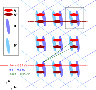
Figure 5: (Color online) Visualization of the full effective Wannier Hamiltonian eq. (1). A schematic drawing of the most dominant hopping processes is presented: type A orbitals (red), type B orbitals (blue). Lines denote the dominant hopping paths, and the black square marks the size of the unit cell.

II.3 Effective inter-chain coupling

The Wannier model eq. (1) consists of numerous single-particle hopping terms between four Wannier orbitals in a three dimensional crystal. Many of the terms of the Wannier model are orders of magnitude smaller than the dominant hopping process of type (A) orbitals along $b$ direction with $t_{AA}\approx-0.35\,$eV. For instance, all intra-unit-cell hybridizations are negligibly small (of order $10^{-4}\,$eV). This includes direct hopping $t_{AA^{\prime}}$ between adjacent chains. The reason for this is that the two orbitals type (A) and (A’) are aligned parallel to each other in the unit cell, with negligible overlap. The hybridization perpendicular to the chains, which is responsible for the dispersion in perpendicular direction, is predominantly mediated through the type (B) orbitals in an (A-B-A) or (A-B-A’) fashion, see Fig. 5. In this section, we derive a two-dimensional model in the $b$-$c$ plane consisting of two degenerate half-filled chains that comprises the fundamental model. The indirect hopping results only in a small effective hopping between the chains, which we estimate perturbatively.

The starting point for perturbation theory is a Hamiltonian, where orbitals of type $A$ and type $B$ are decoupled. For this purpose we define a complete set of projection operators projected Hamiltonians $\hat{\mathcal{H}}_{\alpha\alpha}=\hat{P}_{\alpha}\hat{\mathcal{H}}\hat{P}_{\alpha}$ on the type $\alpha=\{(A),(B)\}$ orbitals. In zero-th order approximation, the hybridization terms are set to zero, $\hat{\mathcal{H}}_{AB}=\hat{\mathcal{H}}_{BA}=0$. For our Wannier model this corresponds to neglecting those matrix elements which are less than ten percent of the largest occurring hopping energy $|t_{\text{max}}|=0.35\,$eV and leads to a Hamiltonian

$$H_{\text{reduced}} =\begin{pmatrix}t_{AA}2\cos{(k_{b}b)}&0\\ 0&\epsilon_{B}+t_{BB}2\cos{(k_{b}b\pm k_{c}c)}\\ \end{pmatrix}\mbox{,}$$ (2)

with $t_{AA}=-0.35$ eV, $t_{BB}=-0.11\,$eV and $\epsilon_{B}=-0.45\,$eV accompanied by the rigid band shift of $\mu=-0.03\,$eV. One has to keep in mind that both bands A and B are doubly degenerate. We will refer to this Hamiltonian as reduced model throughout this work.

Note that the two type (B) orbitals disperse in orthogonal diagonals. The bands crossing the Fermi energy arise due to the two degenerate type (A) orbitals which now represent isolated, one-dimensional chains dispersing in $b$ direction. Due to the missing hybridization between A and B orbitals, fine features of the perpendicular ($c$-direction) dispersion are not reproduced. Nevertheless, despite its simplicity, the band structure and density of states (see Fig. 1) are still described very well. Data in the figure have been obtained using $N_{\text{1.BZ}}=48^{3}$ $k$-points in the first BZ and a numerical broadening of $0^{+}=0.086\,t_{\text{max}}$ for the evaluation of the DOS. We find a bandwidth of the two bands in the vicinity of $\epsilon_{F}$ of $W\approx 1.4$ eV and a Fermi velocity of $v_{F}\approx 0.93\cdot 10^{5}\,\frac{\text{m}}{\text{s}}$.

In order to estimate the effective inter-chain coupling we treat the indirect (A-B-A⁽’⁾) hoppings in second-order perturbation theory. For that purpose we project the full four-orbital Wannier model eq. (1) onto the type (A) bands, foo (e)

$$\hat{\widetilde{\mathcal{H}}}_{AA} =\hat{\mathcal{H}}_{AA}+\hat{\mathcal{H}}_{AB}\left(\omega-\hat{\mathcal{H}}_{BB}\right)^{-1}\hat{\mathcal{H}}_{BA}\,\mbox{.}$$

Upon approximating $\omega$ by the bare eigen-energies of $\hat{\mathcal{H}}_{AA}$, we arrive at a two-orbital model which reproduces the band dispersions of the two bands crossing the Fermi energy (not shown). We note in passing that this two-orbital model can also be obtained by a Wannier construction where the basis is restricting to bands of type A alone.

Keeping the number of hopping terms low, we now perform a fit of $\hat{\widetilde{\mathcal{H}}}_{AA}(\mathbf{k})$ with a Hamiltonian that contains perpendicular hopping in addition to the terms of the (A) orbitals of the reduced model (eq. (2)) respecting the symmetry of the lattice. In particular, we choose for the perpendicular hopping both intra-chain ($A$-$A$) terms as well as inter-chain ($A$-$A^{\prime}$) terms. The $\chi^{2}$ fit is done using $20^{2}$ $k$-points on an equidistant grid in one fourth of the reciprocal $b$-$c$ plane ($k_{a}\approx 0$) plus $3\cdot 32$ $k$-points on the standard path Y-G-X-M. The only relevant perpendicular hopping processes given by this procedure are nearest-neighbor inter-chain terms of the order of $t_{AA^{\prime}}\approx-0.005\,$eV, as well as nearest neighbor intra-chain terms of the order of $t_{AA}\approx-0.02\,$eV. The hopping in $b$ direction only slightly renormalizes to $t_{AA/A^{\prime}A^{\prime}}\approx-0.37\,$eV accompanied by an on-site shift of $\epsilon_{A/A^{\prime}}=-0.01\,$eV.

Thus, we find an intuitive two orbital model that consists of two chains dispersing in $b$ direction with nearest neighbor perpendicular hoppings of type $A$-$A$ and $A^{\prime}$-$A^{\prime}$ which are one order of magnitude smaller than the hopping in $b$ direction. The direct effective hopping of type $A$-$A^{\prime}$ between the two chains within one unit cell is again one order of magnitude smaller. This small effective coupling explains the robust one-dimensionality of the compound. Our calculated values are in good agreement with those discussed in Ref. Chudzinski et al., 2012.

We want to stress here that only in this section fitting of parameters was performed, in order to estimate the effective perpendicular hopping using only a few parameters. In all other parts of this work, only ab-initio calculated hopping integrals are used.

III Anisotropic conductivity

We augment our discussion of the electronic structure by computing the linear response transport and comparing it to experiments.

The conductivity tensor of Li_0.9Mo₆O₁₇ consists of three independent diagonal $\sigma_{a},\sigma_{b},\sigma_{c}$ entries as well as one non-zero off-diagonal element $\sigma_{bc}=\sigma_{cb}$ (see Appendix A).

Ref.	$\rho_{a}$	$\rho_{b}$	$\rho_{c}$	ratio
	m$\Omega$cm	m$\Omega$cm	m$\Omega$cm
Ref. Greenblatt et al.,1984	$2470$	$9.5$	-	260:1:-
Ref. Chen et al.,2010	$64.5$	$16$	$854$	4.5:1:50
Ref. Choi et al.,2004	-	$1.7$	-	-:1:-
Ref. da Luz et al.,2007	$110(40)$	$19(1)$	$47(5)$	6(2):1:2.5(4)
Ref. Mercure et al.,2012a	$30$	$0.4$	$600$	80:1:1600
Ref. Xu et al.,2009	-	$0.4$	-	100:1:$>$100
Ref. Wakeham et al.,2011	-	-	-	100:1:-
full Wannier model	$\approx 430\gamma$	$\approx 1.8\gamma$	$\approx 600\gamma$	240:1:330
reduced model	-	$\approx 2\gamma$	-	-:1:-

Table 1: Collected data for the anisotropic resistivity at $T=300\,$K and our low temperature theoretical results for small scattering $\gamma[$eV$]\sim 0.05\,$eV. Data from Ref. Greenblatt et al., 1984, Ref. Chen et al., 2010 and Ref. Choi et al., 2004 was obtained via four-point measurements, Ref. da Luz et al., 2007 and Ref. Mercure et al., 2012a report results using the Montgomery method, Ref. Xu et al., 2009 measurements are based on magneto resistance and in Ref. Wakeham et al., 2011 a Hall experiment was carried out.

Literature provides values for the anisotropic resistivity at room temperature ($300\,$K) and zero magnetic field using several experimental techniques. We summarized the reported data in Tab. 1 which all agree on a highly anisotropic resistivity. The ratio between the diagonal elements of the resistivity tensor, however, strongly disagrees in between the individual measurements. In particular $\rho_{a}:\rho_{b}$ differs by a factor of $\approx 60$ while $\rho_{b}:\rho_{c}$ differs even by a factor of $\approx 640$ from the lowest to the highest anisotropy found in experiments. These discrepancies are often attributed to experimental challenges when measuring the resistivity of strongly anisotropic small samples. To our knowledge we present the first theoretical study of the conductivity of Li_0.9Mo₆O₁₇.

III.1 Conductivity of the reduced model

The reduced model introduced in eq. (2) consists of $N_{\text{band}}=2$ degenerate bands (type A) crossing the Fermi energy dispersing only in $b$ direction with velocity $v_{b}^{AA}(\mathbf{k})=-\frac{2t_{AA}}{\hbar}b\sin{(k_{b}b)}$ (eq. (12)). In this case of diagonal velocities and spectral functions, the conductivity (see Appendix A.1) becomes

$$\sigma_{bb} =\frac{16e^{2}t_{AA}^{2}}{\hbar}\frac{b^{2}}{ac}\int_{-\infty}^{\infty}d\omega\frac{\beta}{2(1+\cosh{(\beta(\omega-\mu))})}$$

$$\times\int_{0}^{\frac{\pi}{b}}dk_{b}\sin^{2}{(k_{b}b)}(\frac{\gamma}{\pi})^{2}\frac{1}{((\omega-2t_{AA}\cos{(k_{b}b)})^{2}-\gamma^{2})^{2}}\,\mbox{,}$$

where we introduced a phenomenological scattering $\gamma\sim|\Im\text{m}(\Sigma(\omega=\mu))|$ in the Lorentzian-shaped spectral function. In the low-temperature small-scattering limit we find

$$\sigma_{bb} =\frac{16e^{2}t_{AA}^{2}}{\hbar}\frac{b^{2}}{ac}\int_{-\infty}^{\infty}d\omega\delta(\omega-\mu)$$

$$\times\int_{0}^{\frac{\pi}{b}}dk_{b}\sin^{2}{(k_{b}b)}\frac{\delta(\omega-2t_{AA}\cos{(k_{b}b)})}{2\pi\gamma}\,\mbox{,}$$

which evaluates to

$$\sigma_{bb} =\frac{4e^{2}}{h\gamma}\frac{b}{ac}\sqrt{(2t_{AA})^{2}-\mu^{2}} \stackrel{{\scriptstyle\mu=0}}{{\approx}}N_{\text{spin}}N_{\text{band}}\frac{D}{R_{K}\gamma}\frac{b}{ac}\,\mbox{,}$$

with $D=2t_{AA}$ and $R_{K}=\frac{h}{e^{2}}$ the von-Klitzing constant. Using this expression we find for the resistivity $\rho_{bb}=\frac{1}{\sigma_{bb}}\approx 2\gamma[$eV$]\,$m$\Omega$cm. Considering a reasonable mean-free path $d$ of the order of a unit-cell length and using the calculated Fermi velocity of $\approx 10^{5}\,\frac{\text{m}}{\text{s}}$ we can estimate a scattering of $\gamma[$eV$]=\frac{0.658}{d[\AA]}\approx 0.05\,$eV which implies a resistivity of $\rho_{bb}\approx 0.1\,$m$\Omega$cm.

III.2 Conductivity anisotropy

The reduced model is limited to transport in $b$ direction. To study the high transport anisotropy suggested by experiments, we calculate the conductivity tensor of the full four-orbital Wannier model. We evaluate eq. (8) numerically at $T=4.2\,$K and for small scattering $\gamma$ (for details see Appendix A.2). For the resistivity we obtain $\rho_{a}\approx 430\gamma[$eV$]$ m$\Omega$cm, $\rho_{b}\approx 1.8\gamma[$eV$]$ m$\Omega$cm, and $\rho_{c}\approx 600\gamma[$eV$]$ m$\Omega$cm ($\rho_{a}:\rho_{b}:\rho_{c}\sim 240:1:330$). Note that the $b$ axis resistivity in the strictly one-dimensional model eq. (2) is only $\approx 10\%$ larger than the resistivity in the four-orbital model, which means that the reduced model yields already a quite accurate description of the $b$ axis transport. The $a$ and $c$ axis resistivities are roughly two orders of magnitude larger than in $b$ direction, compatible with experimental data. Using the same phenomenological scattering $\gamma\approx 0.05$ as motivated in the previous section we obtain $\rho_{a}\approx 20\,$m$\Omega$cm, $\rho_{b}\approx 0.1\,$m$\Omega$cm and $\rho_{c}\approx 30\,$m$\Omega$cm. The resistivity ratio of $\rho_{a}/\rho_{b}\sim 240$ does compare best to the experimental value $260$ as obtained in Ref. Greenblatt et al., 1984 (see Tab. 1).

IV Correlated electronic structure

The obtained Wannier model is close to being half-filled which indicates that the local part of the Coulomb interactions is most important. The effects of off-diagonal Coulomb interactions are small and further discussed in Appendix B. In the following, we focus on local electron-electron interactions of density-density type, which are added to the ab-initio tight-binding Wannier model

$$\hat{\mathcal{H}} =\hat{\mathcal{H}}_{\text{Wannier}}+\hat{\mathcal{H}}_{\text{int}}\,\mbox{,}$$ (3)

where the single-particle part $\hat{\mathcal{H}}_{\text{Wannier}}$ is defined in eq. (1) and

$$\hat{\mathcal{H}}_{\text{int}} =\sum\limits_{\mathbf{R}}\sum\limits_{\alpha}\,U_{\alpha}\hat{n}_{\mathbf{R}\alpha\uparrow}\hat{n}_{\mathbf{R}\alpha\downarrow}\,\mbox{,}$$ (4)

where $\hat{n}_{\mathbf{R}\alpha\sigma}$ is the particle number operator for Wannier orbital $\alpha=\{A,A^{\prime},B,B^{\prime}\}$ and spin $\sigma=\{\uparrow,\downarrow\}$ in unit cell $\mathbf{R}$. In order to treat the different band fillings in the model properly we employ a simple double counting correctionRyndyk et al. (2012) in $\hat{\mathcal{H}}_{\text{Wannier}}$,

$$M_{\mathbf{0}\alpha\mathbf{0}\alpha}^{+\text{DC}} =M_{\mathbf{0}\alpha\mathbf{0}\alpha}-U_{\alpha}\langle n_{\mathbf{0}\alpha}\rangle_{\text{Wannier}}\,\mbox{,}$$ (5)

where the densities $\langle n\rangle_{\text{Wannier}}$ are taken from the noninteracting Wannier model. Adding interactions we furthermore set the chemical potential $\mu$ such that the average filling of electrons in the system is at its physical value $\langle n\rangle\approx 1.44$.

This interacting theory is challenging to solve, even more so because the expected results hint to low dimensional physics which can promote non-local self-energy effects. We employ two complementary techniques to study on a first, more qualitative level, the effect of interactions. First, we apply the VCA, which contains non-local contributions to the self-energy $\Sigma$. Second, we augment these results by a DMFT calculation which neglects contributions of non-local self-energy terms, but is superior in the treatment of the low-energy quasi-particle resonance.

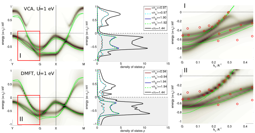
Figure 6: (Color online) Spectral function and DOS of the interacting model. Top row: VCA data for $U=1\,$eV using eight-orbital clusters. Bottom row: DMFT data for $U=1\,$eV. Left: Spectral function plotted along a two dimensional path in the reciprocal $b$-$c$ plane. The noninteracting dispersion is plotted on top (dashed-green). Center: Orbitally resolved density of states. Right: Zoom to the spectral function in the respective red rectangle compared to ARPES data from Ref. Wang et al., 2009 which are indicated as red circles.

IV.1 Variational Cluster Approach

The VCA Potthoff et al. (2003) is a quantum many-body cluster method which is capable of treating short range correlations exactly. Potthoff et al. (2003); Dahnken et al. (2004); Aichhorn et al. (2004); Senechal (2009) The given lattice Hamiltonian is partitioned into a cluster- and an inter cluster-Hamiltonian $\hat{\mathcal{H}}=\hat{\mathcal{H}}^{\text{cl}}+\hat{\mathcal{H}}^{\text{inter}}$, where only single-particle terms are allowed in the inter cluster part (for details see Appendix B). Clusters consist of one or more unit cells and are chosen so that their single-particle Green’s function $g_{ml}^{\sigma}(z)$ can be obtained exactly. We use clusters consisting of two unit cells in $b$ direction ($L_{\mathcal{C}}=8$) to capture at least the most basic non-local self-energy effects on the quasi one-dimensional chains which enable signatures of a possible spin-charge separation. Aichhorn et al. (2005) In this work we employ a numerical Band Lanczos scheme and the Q-matrix formalism to obtain $g_{ml}^{\sigma}(z)$. Aichhorn et al. (2006) The CPT approximation to the single-particle Green’s function of the full system $G^{-1}(z)$ is given within first order strong coupling perturbation theory by Gros and Valenti (1993); Sénéchal et al. (2000)

$$G^{-1}(z)=g^{-1}(z)-H^{\text{inter}}\,\mbox{,}$$ (6)

where $H^{\text{inter}}$ are the matrix elements of the inter cluster Hamiltonian in the basis of cluster orbitals. If the cluster is larger than the actual unit cell of the crystal, we use a Green’s function periodization prescription to project on the original unit cell $G_{\alpha\beta}(z)$ Senechal (2009).

Within VCA, eq. (6) is evaluated at the stationary point of the generalized grand potential $\Omega[\boldsymbol{\Sigma}]$ (for fermions at zero temperature) which is available from $G$ and $g$. Potthoff et al. (2003) The grand potential is parametrized by the VCA variational parameters $\boldsymbol{\Delta}$ which are fixed by the VCA condition Potthoff et al. (2003)

$$\boldsymbol{\nabla}_{\boldsymbol{\Delta}}\Omega(\boldsymbol{\Delta})\stackrel{{\scriptstyle!}}{{=}}\mathbf{0}\,\mbox{.}$$ (7)

The VCA improves the CPT ($\mathbf{\Delta}\equiv\mathbf{0}$) approximation (which is to approximate the self-energy $\Sigma_{G}$ of the full system by the self-energy of the cluster $\Sigma_{g}$) by adding flexibility to the cluster self-energy in terms of variational parameters $\mathbf{\Delta}$. We consider the on-site energies of the four Wannier orbitals as independent variational parameters $\boldsymbol{\Delta}=\{\Delta_{\epsilon_{A}},\Delta_{\epsilon_{A^{\prime}}},\Delta_{\epsilon_{B}},\Delta_{\epsilon_{B^{\prime}}}\}$ (which implicitly includes an overall shift of the chemical potential of the cluster) and use $N_{\text{1.BZ}}=32^{3}$ $k$-points in the irreducible BZ for the evaluation of eq. (7).

Advantages of the VCA are that i) it is exact in the noninteracting system, ii) the approximation is systematically improvable by enlarging cluster sizes, iii) or increasing the number of variational parameters $\mathbf{\Delta}$ and iv) it is possible to work directly in the real energy domain as well as in Matsubara space. VCA on small clusters is inherently biased towards the insulating state, therefore we expect to overestimate a possible Mott gap (see Appendix C for a discussion).

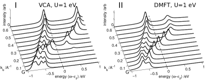
Figure 7: (Color online) Cuts through the spectral function along the $b$ axis. The parameters and labels (I, II) correspond to those in Fig. 6.

IV.2 Dynamical Mean Field Theory

A complementary approach that neglects non-local effects but describes the local dynamical quantum fluctuations better is the DMFT. Georges et al. (1996) Within this theory the interacting lattice problem is mapped on a self-consistent four-orbital impurity model coupled to an infinite electronic bath. The DMFT approximation is to assume a momentum-independent self-energy of the original model $\Sigma_{\alpha\beta}$

$$\Sigma_{\alpha\beta}(i\omega,\mathbf{k}) \stackrel{{\scriptstyle!}}{{=}}\mathcal{S}_{\alpha\beta}(i\omega)\,\mbox{,}$$

where $\mathcal{S}_{\alpha\beta}$ is the local self-energy generated by the auxiliary quantum impurity system.

As impurity solver we use the continuous time Quantum Monte Carlo (CT-QMC) code of the TRIQS Ferrero and Parcollet toolkit and its implementation of the hybridization expansion (CT-HYB) Werner et al. (2006); Werner and Millis (2006) algorithm using Legendre polynomials. Boehnke et al. (2011) This sign-problem free method works in Matsubara space and provides statistically exact and reliable results even at very low temperatures. Gull et al. (2011) We used a low temperature of $\beta=150\,$eV^-1 and a $k$-mesh of $N_{\text{1.BZ}}=800$. The imaginary time data is continued to the real frequency axis using a parallel tempering analytic continuation method. Beach

Different to VCA, the DMFT as applied here neglects non-local correlations. On the other hand, it treats the local dynamical quantum fluctuations accurately.

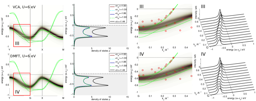
Figure 8: (Color online) Spectral function and DOS of the interacting model for high values of on-site interaction strength as one would expect for atomic like molybdenum $d$ orbitals: $U=6\,$eV. For legends, arrangement of the subplots and color coding see Fig. 6. On the far right we show cuts through the spectral function as in Fig. 7.

IV.3 Discussion of the interacting dynamics

For models based on atomic orbitals, constrained LDA calculations suggest an on-site interaction for the atomic $d$ Mo orbitals of $U\approx 6.4$ eV and a nearest-neighbor interaction of $V\approx 0.2\,$eV Popović and Satpathy (2006) in Li_0.9Mo₆O₁₇, while the bulk Mo value for the on-site interaction is $U\approx 3.8\,$eV. Chudzinski et al. (2012) As we will discuss below, in our model these larger interaction values $U$, which have been proposed and used for model calculations, Merino and McKenzie (2012); Chudzinski et al. (2012) do not give results in accordance with experimental data. Obtaining the interaction parameters in an ab-inito way by, e.g. the constrained Random Phase Approximation (cRPA), Miyake et al. (2009); Imada and Miyake (2010) would be highly desirable, but is beyond our present computational capabilities due to the very large unit cell of the system.

In the following, based on physical arguments, we will nevertheless argue that a moderate value of $U$ is appropriate for our model. We use uniform on-site interactions $U_{\alpha}=U$ only and estimate the magnitude of the interaction strength to be of the order of a few $t_{\text{max}}$. The reduced value, compared to the atomic one, can be motivated by i) the large spread of the orbitals, Ferber et al. and ii) the effective screening of other Mo 4d states near the Fermi level. We want to remind the reader that we are not dealing with atomic orbitals (where for molybdenum the interaction $U$ could be of the order of several electron volts) but with extended, even molecular-like, orbitals (see Fig. 4).

Let us start the discussion using interaction values of the order of the band width, i.e. using $U=1$ eV. We show results for the single-particle spectrum and orbitally resolved DOS of the interacting model in Fig. 6 (left and center) and Fig. 7. foo (f) We used a Lorentzian broadening of $0^{+}=0.05$ eV for plotting the spectral functions, as well as $0^{+}=0.025$ eV for plotting the DOS. As discussed in the previous section, the VCA is biased towards an insulating solution (see also Appendix C), that is why there is a small gap in the conduction band visible in the spectral function, which is not seen in the DMFT results.

Comparing the single-particle dynamics to recent experiments (ARPES data from  Ref. Wang et al., 2009 and  Ref. Wang et al., 2006) we find very good agreement for the bands at the Fermi energy (Fig. 6 (right)). The renormalization of the effective mass of the half-filled orbitals, calculated from the DMFT self energy, is $m\approx 1.2m_{0}$, where $m_{0}$ is the LDA band mass.

Regarding the bands crossing the Fermi energy, their slope improves in VCA/DMFT with respect to the LDA data, and compares well with the measured excitations in ARPES experiments.Wang et al. (2009) Note that the up-most branch provides only a very weak signal in the ARPES data as compared to the lower branch. In our DMFT calculation, the electronic correlations suppress the hybridizations between chains (A) and (A’), making them equivalent. This leads to only one dispersing feature crossing the Fermi energy, see Fig. 6 lower right panel. The red circles at lower binding energy correspond to the shoulder in the ARPES data, which are very likely due to non-local correlation effects that are completely neglected in the single-site DMFT approach. A final statement on the impact of non-locality of the self energy and spin-charge separation on the single-particle excitations require a detailed investigation on large systems, which is beyond the scope of this paper.

Increasing the interaction value further, for instance to $U=1.5$ eV does not change results significantly (left aside the artificial gap in the VCA calculation). Above a certain limit, however, which is around $U=2.5$ eV in our calculations, a Mott gap opens in the two half-filled bands. An extreme example is using the atomic value for the interaction, $U=6$ eV, which is shown in Fig. 8. The half-filled bands are in the Mott insulating state, with the spectral weight transferred to roughly $\pm 3\,$eV. The only spectral weight left close to the Fermi level originates from the two almost filled orbitals, type (B). This is of course qualitatively different from experimental results.

The values of $U$ given here can only be seen as rough estimates to the actual value, and are by no means ab-initio. The DMFT overestimates the metallicity of a system, in particular in low dimensions while the VCA underestimates it. Hence, using different techniques which are tailored more towards low dimensions, the needed value of $U$ to open a Mott gap might be even smaller. As has been shown by Chudzinski et al., Chudzinski et al. (2012) the system should be metallic, but very close to an insulating state. Our observations can be used as guideline in further studies to determine the value of $U$. At very large coupling $U=6$ eV, however, the system as modeled here is strongly localized, and the insulating state there should be very robust. This is supported by the fact that both methods, VCA and DMFT, give indistinguishable results in this (almost) atomic limit. It clearly shows that taking atomic values for $U$ is inadequate for the effective model derived in this work.

Let us shortly comment on the effect of correlations in the reduced model, Sec. II.3. There, the Hamiltonian of the half-filled and the filled bands decouples exactly, which means that one is left with a standard one-dimensional (almost) half-filled Hubbard model with nearest-neighbor hopping only. Essler et al. (2010) As discussed in Sec. II.3 and Sec. III.1, this gives a quite good description of the dispersion in chain-direction including transport properties. Effects beyond the one-dimensional Hubbard model can be included using the effective perpendicular hopping terms as estimated in Sec. II.3. In a recent study on dimensional crossoverRaczkowski and Assaad (2012) the critical perpendicular coupling to enter the regime of one-dimensional physics is $t_{p}\approx 0.18t$ at interaction strength $U=3t$. Of course, this value depends on model details such as frustrated hopping and interaction strength. However, since our estimated value for $t_{p}$ in Li_0.9Mo₆O₁₇ is significantly smaller than this boundary, we suggest that this can explain the robustness of 1D physics in this compound. We leave a more detailed study of the dimensional crossover in Li_0.9Mo₆O₁₇ for further investigations.

V Conclusions

We have devised a model for the electronic structure of the highly anisotropic low dimensional purple bronze Li_0.9Mo₆O₁₇. Starting from ab-initio calculations, applying Density Functional Theory in the Local Density Approximation, we constructed a four-orbital model based on molybdenum $d$ states in terms of maximally localized Wannier functions. This leads to an effective theory with two filled bands slightly below and two half-filled bands crossing the Fermi energy. We obtained an even more elementary effective model with reduced dimensionality consisting of two orbitals only, tailored towards studies of interactions at low energies.

We showed that basic electronic properties of our model are in good agreement with experimental data and ab-initio results. Estimated anisotropic transport coefficient reproduce experimental trends. The model enables us to study effects of many-body correlations. In a first approach we made use of the (extended) Variational Cluster Approach which takes into account non-local contributions to the self-energy and Dynamical Mean Field Theory to study the effects of density-density type electron-electron interactions. Our results indicate that moderate on-site interactions (of the order of the band width) are essential while nearest-neighbor density-density interactions play a minor role. The so obtained single-particle spectra agree well with recent angle resolved photo emission experiments. Our study sets some qualitative limits on the value of the interaction parameters. In particular, we could show that the values used for atomic-like molybdenum $d$ orbitals are completely inappropriate for our Wannier model of lithium purple bronze.

We would like to point out that our model is very different from previously proposed descriptions for Li_0.9Mo₆O₁₇ which were based on atomic orbitals with a comparatively high on-site interaction strength of several electron volts. We suggest that low-energy treatments of this one-dimensional model should start from two half-filled chains with moderate on-site interaction rather than quarter-filled ladder models with high values of on-site interaction strength plus off diagonal interactions.

Our model is intended to serve as a starting point for future studies of the electronic structure and interactions of Li_0.9Mo₆O₁₇ be it in a renormalization group - Luttinger liquid or computational many-body sense. On the latter side it would certainly be interesting to conduct a more thorough investigation of non-local self-energy effects to complement our (extended) Variational Cluster Approach results. In particular, the phenomenon of spin-charge separation deserves further attention. A theoretical understanding of the phase diagram of the system, i.e., the occurrence of superconducting, insulating, or charge ordered states as function of pressure and temperature, remains a challenging open question. These studies could be augmented by an ab-inito calculation of interaction parameters for the Wannier model by appropriate techniques such as constrained Random Phase Approximation, Imada and Miyake (2010); Miyake et al. (2009) making the approach fully ab-initio. At the moment of writing, this is not feasible due to the computational complexity.

Appendix A Linear response transport

The structure of the conductivity tensor $\sigma_{\alpha\beta}$ of Li_0.9Mo₆O₁₇ follows from the $C_{2h}$ point symmetry as well as physical symmetry considerations for the conductivity Hartmann (1984) and can easily be established by requiring the conductivity tensor to be i) symmetric for physical reasons and ii) invariant under transformations with the four lattice point symmetry operations (identity, inversion, mirror symmetry perpendicular to $a$-axis and two fold rotation around the $a$-axis) $S_{\alpha}$: $\sigma=S_{\alpha}\sigma S_{\alpha}^{T}$.

A.1 Formalism

Following Refs. Oudovenko et al., 2006; Tomczak and Biermann, 2009; Deng and Mravlje, 2012, linear response transport coefficients can be expressed in terms of kinetic coefficients

$$\mathcal{A}^{n}_{\nu\mu} =N_{\text{spin}}\pi\hbar\int\limits_{-\infty}^{\infty}d\omega\,(\beta\omega)^{n}$$

$$\times p_{\text{FD}}(\omega,\mu,\beta)p_{\text{FD}}(-\omega,-\mu,\beta)\Gamma_{\nu\mu}(\omega,\omega)\,\mbox{,}$$ (8)

where $N_{\text{spin}}=2$ is due to spin degeneracy, the indices $\nu,\mu=\{a,b,c\}$ denote the real space coordinate system, and we neglect vertex corrections. The Fermi-Dirac distribution $p_{\text{FD}}(\omega,\mu,\beta)=\frac{1}{e^{\beta(\omega-\mu)}+1}$ restricts the interval of integration to $\beta^{-1}\sim k_{B}T$ around the Fermi energy $\epsilon_{F}$ ($k_{B}$ is Boltzmann’s constant, and $T$ and $\beta$ denote temperature and inverse temperature, resp.). The transport distribution

$$\Gamma_{\nu\mu}(\omega_{1},\omega_{2}) =\frac{1}{V}\frac{1}{N_{\text{1.BZ}}}\sum\limits_{\mathbf{k}\in 1.\text{BZ}}\text{Tr}$$

$$\times{\left[v_{\nu}(\mathbf{k})A(\omega_{1},\mathbf{k})v_{\mu}(\mathbf{k})A(\omega_{2},\mathbf{k})\right]}\,\mbox{,}$$ (9)

($V=abc$ is the unit cell volume) is given in terms of the velocities

$$v_{\nu}^{\alpha\beta}(\mathbf{k}) =-\frac{\hbar}{m}\mathinner{\langle{\Psi_{\alpha}(\mathbf{k})}|}\nabla_{\nu}\mathinner{|{\Psi_{\beta}(\mathbf{k})}\rangle}\,\mbox{,}$$ (10)

and the spectral function

$$A_{\alpha\beta}(\omega,\mathbf{k}) =-\frac{1}{\pi}\Im{\text{m}(G^{R}_{\alpha\beta}(\omega,\mathbf{k}))}\,\mbox{,}$$ (11)

which both are matrices in orbital indices $\alpha,\beta=\{A,A^{\prime},B,B^{\prime}\}$, which the trace Tr runs over.

We use velocities $v_{\nu}^{\alpha\beta}(\mathbf{k})$ (eq. (10)) in the Peierls approximation (neglecting the gradient of the Wannier orbital itself leading to a diagonal representation)

$$v_{\nu}^{\alpha\beta}(\mathbf{k}) =\frac{1}{\hbar}\Bigg{(}\mathinner{\langle{\omega_{\alpha}(\mathbf{k})}|}\frac{\partial\hat{\mathcal{H}}(\mathbf{k})}{\partial k_{\nu}}\mathinner{|{\omega_{\beta}(\mathbf{k})}\rangle}$$

$$-{\rm\alpha}\left(r_{\alpha}-r_{\beta}\right)\mathinner{\langle{\omega_{\alpha}(\mathbf{k})}|}\hat{\mathcal{H}}(\mathbf{k})\mathinner{|{\omega_{\beta}(\mathbf{k})}\rangle}\Bigg{)}$$

$$\approx\frac{1}{\hbar}\frac{\partial E_{\alpha}(\mathbf{k})}{\partial k_{\nu}}\delta_{\alpha\beta}$$ (12)

where the second term in the first expression takes intra-unit cell processes into account, Tomczak and Biermann (2009) and $r_{\alpha}$ is the position of Wannier orbital $\alpha$ inside the unit cell. This term is neglected in the following because the intra-unit cell hopping elements are negligibly small.

The conductivity tensor is

$$\sigma_{\nu\mu} =\beta e^{2}\mathcal{A}_{\nu\mu}^{0}\,\mbox{,}$$ (13)

with $e$ denoting the electron charge.

A.2 Details on the evaluation of the anisotropic conductivity

In this appendix we outline the numerical procedure used for the evaluation of the conductivity tensor eq. (13). These equations contain four additional, auxiliary numerical parameters in which we converge our results: i) The spectral function $A_{\alpha\beta}(\omega,\mathbf{k})$ (eq. (11)) of the Wannier Hamiltonian is available exactly through the noninteracting retarded single-particle Green’s function $G_{\alpha\beta}^{R}(\omega)=\mathinner{\langle{\omega_{\alpha}(\mathbf{k})}|}\frac{1}{\omega+i\gamma-\hat{\mathcal{H}(\mathbf{k})}}\mathinner{|{\omega_{\beta}(\mathbf{k})}\rangle}$. The broadening $\gamma$ of the spectral function is chosen phenomenologically as described in the man part of the text. For numerical reasons $\gamma$ has to be chosen in accordance with, ii) the number of $k$-points $N_{\text{1.BZ}}$ in the first BZ for the sum in eq. (9). We obtain converged conductivities for $N_{\text{1.BZ}}^{1/3}\in[1,67]$ to within a relative error of $10^{-3}$ using an equidistant grid in the irreducible BZ. We use $\gamma=\{0.1,0.075,0.05,0.025\}$ and rescale all conductivities with $\gamma$. As a function of $\gamma$, the resistivities in $a$ and $b$ direction are constant at $\rho_{a}\approx(1.8\pm 0.05)\gamma$ and $\rho_{b}\approx(430\pm 10)\gamma$ while the resistivity in $c$ direction shows an upwards trend. For our values of $\gamma$ we find $\rho_{c}\approx\{190,300,480,650\}\gamma$. Since the last data point at $\gamma=0.025$ is already difficult to converge in $N_{\text{1.BZ}}$ we estimate $\rho_{c}\approx(600\pm 150)\gamma$.

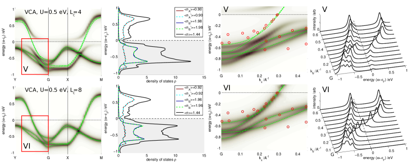
Figure 9: (Color online) Comparison of VCA cluster sizes for a moderate on-site interaction strength of $U=0.5\,$eV. Top row: VCA data for using four-orbital clusters. Bottom row: VCA data for using eight-orbital clusters. For legends, arrangement of the subplots and color coding see Fig. 8.

iii) The velocities $v_{\nu}^{\alpha\beta}(\mathbf{k})$ (eq. (10)) are obtained by symmetric first order numeric gradient approximations $v_{\nu}^{\alpha\beta}(\mathbf{k})\approx\frac{\delta_{\alpha\beta}}{\hbar}\frac{E_{\alpha}(\mathbf{k}+\frac{\delta}{2}\mathbf{e}_{\nu})-E_{\alpha}(\mathbf{k}-\frac{\delta}{2}\mathbf{e}_{\nu})}{\delta}$ ($\mathbf{e}_{\nu}$ denotes the unit vector in real space dimension $\nu$). The parameter of the finite difference scheme for the velocities used is $\delta=10^{-6}$ after finding only negligible changes in a range of $\delta\in[10^{-8},10^{-3}]$. iv) For reasons of numerical stability we evaluate eq. (13) at a low, but finite temperature of $T=4.2\,K$, keeping in mind that $v_{\nu}^{ij}(\mathbf{k})$ and $A(\omega,\textbf{k})$ have been evaluated for zero temperature. We find the results to be independent of this choice in a range of $T\in[1,50]\,K$. In this calculation, at fixed $\gamma,$ the temperature dependence enters through the Fermi-Dirac distribution only and a small scattering is taken into account through the broadening $\gamma$ in the spectral function. We checked the numeric procedure on the reduced model where analytic results are known (see main text).

Appendix B Non-local interactions - extended VCA

Here we outline the VCA theory as implemented to obtain the results of the main text including the extensions needed in eVCA to treat non-local Coulomb interactions.Aichhorn et al. (2004) The single-particle part of the full Hamiltonian is readily decomposed into a cluster and an inter cluster part

$$\hat{\mathcal{H}}_{\text{Wannier}}^{\text{cl}} =M_{\mathbf{\mathcal{R}}m\mathbf{\mathcal{R}}l}\mathinner{|{\omega_{m}}\rangle}\mathinner{\langle{\omega_{l}}|}$$

$$\hat{\mathcal{H}}_{\text{Wannier}}^{\text{inter}} =\sum\limits_{\mathbf{\delta\mathcal{R}}}e^{-i\mathbf{k}\cdot\mathbf{\delta\mathcal{R}}}M_{\mathbf{\mathcal{R}}m\mathbf{\mathcal{R}^{\prime}}l}\mathinner{|{\omega_{m}}\rangle}\mathinner{\langle{\omega_{l}}|}\,\mbox{,}$$

where indices $m$ and $l$ run over the $L_{\mathcal{C}}$ orbitals in the cluster $\mathcal{C}$ at superlattice Senechal (2009) position $\mathbf{\mathcal{R}}$.

When off-diagonal interaction terms are non zero, an additional mean-field treatment is needed for those two-particle terms which extend over the cluster boundary. Aichhorn et al. (2004) This leads to a modified interaction part of the Hamiltonian

$$\hat{\mathcal{H}}_{\text{int}} =\sum\limits_{\mathcal{C}}\left(\hat{\mathcal{H}}_{\text{int}}^{\text{cl}}+\hat{\mathcal{H}}_{\text{mf}}^{\text{cl}}(\boldsymbol{\varphi})\right)$$

$$\hat{\mathcal{H}}_{\text{int}}^{\text{cl}} =\sum\limits_{m=1}^{L_{\mathcal{C}}}\,U_{m}\,\hat{n}_{m\uparrow}\hat{n}_{m\downarrow}+\sum\limits_{\begin{subarray}{c}m<l\in\mathcal{C}\\ \sigma\sigma^{\prime}\end{subarray}}\,V_{ml}\,\hat{n}_{m\sigma}\hat{n}_{l\sigma^{\prime}}$$

$$\hat{\mathcal{H}}_{\text{mf}}^{\text{cl}}(\boldsymbol{\varphi}) =\sum\limits_{ml}\,\widetilde{V}_{ml}\left(\sum\limits_{\sigma}\left(\hat{n}_{m\sigma}\varphi_{l}+\hat{n}_{l\sigma}\varphi_{m}\right)-\varphi_{l}\varphi_{m}\right)\,\mbox{,}$$

with on-site interaction strength $U_{m}$, intra-cluster off-diagonal interactions $V_{ml}$ as well as $\widetilde{V}_{ml}=\sum\limits_{\mathbf{\mathcal{R}}}V_{0m\mathbf{\mathcal{R}}l}$ the interaction elements in the mean-field Hamiltonian. The mean-fields $\boldsymbol{\varphi}$ (taken as spin independent $\varphi_{m}=\sum\limits_{\sigma}\langle\hat{n}_{m\sigma}\rangle$ and restricted by lattice symmetry) need to be determined self-consistently.

This allows to write the (interacting) cluster Hamiltonian in the VCA as

$$\hat{\mathcal{H}}^{\text{cl}}(\boldsymbol{\Delta},\boldsymbol{\varphi}) =\hat{\mathcal{H}}^{\text{cl}}_{\text{Wannier}}(\boldsymbol{\Delta})+\hat{\mathcal{H}}^{\text{cl}}_{\text{int}}+\hat{\mathcal{H}}^{\text{cl}}_{\text{mf}}(\boldsymbol{\varphi})\,\mbox{,}$$

where we introduced the VCA variational parameters Potthoff et al. (2003); Dahnken et al. (2004) $\boldsymbol{\Delta}$.

To study the impact of non-local Coulomb interactions we extend eq. (4) by

$$\hat{\mathcal{H}}_{\text{int,nl}} =\hat{H}_{\text{int}}+\sum\limits_{\mathbf{R}<\mathbf{R^{\prime}}}\sum\limits_{\begin{subarray}{c}\alpha<\beta\\ \sigma\sigma^{\prime}\end{subarray}}\,V_{\mathbf{R}\alpha\mathbf{R^{\prime}}\beta}\,\hat{n}_{\mathbf{R}\alpha\sigma}\hat{n}_{\mathbf{R^{\prime}}\beta\sigma^{\prime}}\,\mbox{,}$$

which also effects the double counting terms in eq. (5)

$$M_{\mathbf{0}\alpha\mathbf{0}\alpha}^{+\text{DC,nl}} =M_{\mathbf{0}\alpha\mathbf{0}\alpha}^{+\text{DC}}-\sum\limits_{\mathbf{R}\gamma}V_{\mathbf{0}\alpha\mathbf{R}\gamma}\langle n_{\mathbf{R}\gamma}\rangle_{\text{Wannier}}\,\mbox{,}$$

where the sum over $(\mathbf{R},\gamma)$ runs over all bonds connected to orbital $(\mathbf{0},\alpha)$. The mean-fields $\boldsymbol{\varphi}$ Aichhorn et al. (2004) which arise due to off-diagonal interaction terms are fixed by the eVCA condition on the generalized grand potential foo (g)

$$\boldsymbol{\nabla}_{\boldsymbol{\Delta},\boldsymbol{\varphi}}\Omega(\boldsymbol{\Delta},\boldsymbol{\varphi})\stackrel{{\scriptstyle!}}{{=}}\mathbf{0}\,\mbox{.}$$

In order to check the influence of nearest-neighbor density-density interactions $V_{\mathbf{R}\alpha\mathbf{R}^{\prime}\beta}$ we did several eVCA calculations with different values within reasonable limits, i.e. below a value of $\approx\frac{U}{2}$. Our calculations show, however, that these interactions $V_{\mathbf{R}\alpha\mathbf{R}^{\prime}\beta}$ lead only to minor differences compared to results without them. We did not find the system to be susceptible to any charge ordering. For that reason, and also because the precise value of the parameters $V_{\mathbf{R}\alpha\mathbf{R}^{\prime}\beta}$ is complicated to estimate, all results presented here are calculate with on-site interaction $U_{\alpha}=U$ only. foo (h) Given the band filling factors and the good agreement with ARPES experiments we argue that on-site interactions are sufficient to describe the spectral properties of this system within our approximation.

Appendix C VCA cluster size extrapolation

Here we discuss the approximation introduced by choosing eight-orbital clusters for the VCA procedure. Eight-orbital clusters enable non-local self-energy effects along the chain direction in the most basic fashion. The VCA on small cluster sizes is inherently biased towards the insulating state. Senechal (2009) In Fig. 9 we show the behavior of the results when going from one-unit cell clusters $L_{\mathcal{C}}=4$ to two-unit cell clusters in $b$ direction $L_{\mathcal{C}}=8$. For the same interaction strength the $L_{\mathcal{C}}=4$ calculation clearly shows a pronounced Mott gap in the (A) type orbitals while it is still absent in the $L_{\mathcal{C}}=8$ calculation. All other basic features are comparable. For numerical reasons we can not go to larger cluster sizes. Nevertheless we expect the results of the $L_{\mathcal{C}}=8$ calculation to be still heavily biased towards the insulating state. One can regard the critical value $U\approx 0.7\,$eV for which the gap opens at $L_{\mathcal{C}}=8$ as a lower bound to the true critical interaction.

References

- McCarroll and Greenblatt (1984) W. McCarroll and M. Greenblatt, Journal of Solid State Chemistry 54, 282 (1984).
- Greenblatt (1988) M. Greenblatt, Chemical Reviews 88, 31 (1988).
- Onoda et al. (1987) M. Onoda, K. Toriumi, Y. Matsuda, and M. Sato, Journal of Solid State Chemistry 66, 163 (1987).
- da Luz et al. (2011) M. S. da Luz, J. J. Neumeier, C. A. M. dos Santos, B. D. White, H. J. I. Filho, J. B. Leão, and Q. Huang, Phys. Rev. B 84, 014108 (2011).
- Greenblatt et al. (1984) M. Greenblatt, W. McCarroll, R. Neifeld, M. Croft, and J. Waszczak, Solid State Communications 51, 671 (1984).
- da Luz et al. (2007) M. S. da Luz, C. A. M. dos Santos, J. Moreno, B. D. White, and J. J. Neumeier, Phys. Rev. B 76, 233105 (2007).
- Mercure et al. (2012a) J.-F. Mercure, A. F. Bangura, X. Xu, N. Wakeham, A. Carrington, P. Walmsley, M. Greenblatt, and N. E. Hussey, Phys. Rev. Lett. 108, 187003 (2012a).
- Xu et al. (2009) X. Xu, A. F. Bangura, J. G. Analytis, J. D. Fletcher, M. M. J. French, N. Shannon, J. He, S. Zhang, D. Mandrus, R. Jin, et al., Phys. Rev. Lett. 102, 206602 (2009).
- dos Santos et al. (2008) C. A. M. dos Santos, M. S. da Luz, Y.-K. Yu, J. J. Neumeier, J. Moreno, and B. D. White, Phys. Rev. B 77, 193106 (2008).
- Matsuda et al. (1986a) Y. Matsuda, M. Sato, M. Onoda, and K. Nakao, Journal of Physics C: Solid State Physics 19, 6039 (1986a).
- Filippini et al. (1989) C. E. Filippini, J. Beille, M. Boujida, J. Marcus, and C. Schlenker, Physica C: Superconductivity 162–164, Part 1, 427 (1989).
- Chen et al. (2010) H. Chen, J. J. Ying, Y. L. Xie, G. Wu, T. Wu, and X. H. Chen, EPL 89, 67010 (2010).
- dos Santos et al. (2007) C. A. M. dos Santos, B. D. White, Y.-K. Yu, J. J. Neumeier, and J. A. Souza, Phys. Rev. Lett. 98, 266405 (2007).
- Choi et al. (2004) J. Choi, J. L. Musfeldt, J. He, R. Jin, J. R. Thompson, D. Mandrus, X. N. Lin, V. A. Bondarenko, and J. W. Brill, Phys. Rev. B 69, 085120 (2004).
- Degiorgi et al. (1988) L. Degiorgi, P. Wachter, M. Greenblatt, W. H. McCarroll, K. V. Ramanujachary, J. Marcus, and C. Schlenker, Phys. Rev. B 38, 5821 (1988).
- Cohn et al. (2012a) J. L. Cohn, B. D. White, C. A. M. dos Santos, and J. J. Neumeier, Phys. Rev. Lett. 108, 056604 (2012a).
- Wakeham et al. (2011) N. Wakeham, A. F. Bangura, X. Xu, J.-F. Mercure, M. Greenblatt, and N. E. Hussey, Nat. Comm. 2, 1 (2011).
- Boujida et al. (1988) M. Boujida, C. Escribe-Filippini, J. Marcus, and C. Schlenker, Physica C: Superconductivity 153–155, Part 1, 465 (1988).
- Chakhalian et al. (2005) J. Chakhalian, Z. Salman, J. Brewer, A. Froese, J. He, D. Mandrus, and R. Jin, Physica B: Condensed Matter 359–361, 1333 (2005), proceedings of the International Conference on Strongly Correlated Electron Systems.
- Denlinger et al. (1999) J. D. Denlinger, G.-H. Gweon, J. W. Allen, C. G. Olson, J. Marcus, C. Schlenker, and L.-S. Hsu, Phys. Rev. Lett. 82, 2540 (1999).
- Wang et al. (2006) F. Wang, J. V. Alvarez, S.-K. Mo, J. W. Allen, G.-H. Gweon, J. He, R. Jin, D. Mandrus, and H. Hochst, Phys. Rev. Lett. 96, 196403 (2006).
- Wang et al. (2009) F. Wang, J. V. Alvarez, J. W. Allen, S.-K. Mo, J. He, R. Jin, D. Mandrus, and H. Hochst, Phys. Rev. Lett. 103, 136401 (2009).
- Gweon et al. (2003) G.-H. Gweon, J. W. Allen, and J. D. Denlinger, Phys. Rev. B 68, 195117 (2003).
- Gweon et al. (2004) G.-H. Gweon, S.-K. Mo, J. W. Allen, J. He, R. Jin, D. Mandrus, and H. Hochst, Phys. Rev. B 70, 153103 (2004).
- Wang et al. (2008) F. Wang, J. Alvarez, S.-K. Mo, J. Allen, G.-H. Gweon, J. He, R. Jin, D. Mandrus, and H. Hochst, Physica B: Condensed Matter 403, 1490 (2008).
- Dudy et al. (2013) L. Dudy, J. D. Denlinger, J. W. Allen, F. Wang, J. He, D. Hitchcock, A. Sekiyama, and S. Suga, Journal of Physics: Condensed Matter 25, 014007 (2013).
- Gweon et al. (2002) G.-H. Gweon, J. Denlinger, C. Olson, H. Hochst, J. Marcus, and C. Schlenker, Physica B: Condensed Matter 312–313, 584 (2002).
- Gweon et al. (2000) G.-H. Gweon, J. D. Denlinger, J. W. Allen, C. G. Olson, H. Hochst, J. Marcus, and C. Schlenker, Phys. Rev. Lett. 85, 3985 (2000).
- Hager et al. (2005) J. Hager, R. Matzdorf, J. He, R. Jin, D. Mandrus, M. A. Cazalilla, and E. W. Plummer, Phys. Rev. Lett. 95, 186402 (2005).
- Podlich et al. (2013) T. Podlich, M. Klinke, B. Nansseu, M. Waelsch, R. Bienert, J. He, R. Jin, D. Mandrus, and R. Matzdorf, Journal of Physics: Condensed Matter 25, 014008 (2013).
- Giamarchi (2004) T. Giamarchi, Chemical Reviews 104, 5037 (2004).
- Pustilnik et al. (2006) M. Pustilnik, M. Khodas, A. Kamenev, and L. I. Glazman, Phys. Rev. Lett. 96, 196405 (2006).
- Khodas et al. (2007) M. Khodas, M. Pustilnik, A. Kamenev, and L. I. Glazman, Phys. Rev. B 76, 155402 (2007).
- Meden and Schönhammer (1992) V. Meden and K. Schönhammer, Phys. Rev. B 46, 15753 (1992).
- Voit (1993) J. Voit, Phys. Rev. B 47, 6740 (1993).
- León et al. (2007) G. León, C. Berthod, and T. Giamarchi, Phys. Rev. B 75, 195123 (2007).
- Xue et al. (1999) J. Xue, L.-C. Duda, K. E. Smith, A. V. Fedorov, P. D. Johnson, S. L. Hulbert, W. McCarroll, and M. Greenblatt, Phys. Rev. Lett. 83, 1235 (1999).
- Biermann et al. (2001) S. Biermann, A. Georges, A. Lichtenstein, and T. Giamarchi, Phys. Rev. Lett. 87, 276405 (2001).
- Berthod et al. (2006) C. Berthod, T. Giamarchi, S. Biermann, and A. Georges, Phys. Rev. Lett. 97, 136401 (2006).
- Raczkowski and Assaad (2012) M. Raczkowski and F. F. Assaad, Phys. Rev. Lett. 109, 126404 (2012).
- Schlenker et al. (1985) C. Schlenker, H. Schwenk, C. Escribe-Filippini, and J. Marcus, Physica B+C 135, 511 (1985).
- Matsuda et al. (1986b) Y. Matsuda, M. Onoda, and M. Sato, Physica B+C 143, 243 (1986b).
- Ekino et al. (1987) T. Ekino, J. Akimitsu, Y. Matsuda, and M. Sato, Solid State Communications 63, 41 (1987).
- Mercure et al. (2012b) J.-F. Mercure, A. F. Bangura, X. Xu, N. Wakeham, A. Carrington, P. Walmsley, M. Greenblatt, and N. E. Hussey, arXiv:1203.6672 (2012b).
- Sato et al. (1987) M. Sato, Y. Matsuda, and H. Fukuyama, Journal of Physics C: Solid State Physics 20, L137 (1987).
- Gweon et al. (2001) G.-H. Gweon, J. Denlinger, J. Allen, R. Claessen, C. Olson, H. Hochst, J. Marcus, C. Schlenker, and L. Schneemeyer, Journal of Electron Spectroscopy and Related Phenomena 117–118, 481 (2001), strongly correlated systems.
- Dumas and Schlenker (1993) J. Dumas and C. Schlenker, International Journal of Modern Physics B 07, 4045 (1993).
- Chudzinski et al. (2012) P. Chudzinski, T. Jarlborg, and T. Giamarchi, Phys. Rev. B 86, 075147 (2012).
- Merino and McKenzie (2012) J. Merino and R. H. McKenzie, Phys. Rev. B 85, 235128 (2012).
- Cohn et al. (2012b) J. L. Cohn, P. Boynton, J. S. Triviño, J. Trastoy, B. D. White, C. A. M. dos Santos, and J. J. Neumeier, Phys. Rev. B 86, 195143 (2012b).
- Whangbo and Canadell (1988) M. H. Whangbo and E. Canadell, Journal of the American Chemical Society 110, 358 (1988).
- Popović and Satpathy (2006) Z. S. Popović and S. Satpathy, Phys. Rev. B 74, 045117 (2006).
- Jarlborg et al. (2012) T. Jarlborg, P. Chudzinski, and T. Giamarchi, Phys. Rev. B 85, 235108 (2012).
- Slater and Koster (1954) J. C. Slater and G. F. Koster, Phys. Rev. 94, 1498 (1954).
- Marzari et al. (2012) N. Marzari, A. A. Mostofi, J. R. Yates, I. Souza, and D. Vanderbilt, Rev. Mod. Phys. 84, 1419 (2012).
- Marzari et al. (2003) N. Marzari, S. I., and V. D., Psi-K Scientific Highlight of the Month 57 (2003).
- Schollwöck (2011) U. Schollwöck, Annals of Physics 326, 96 (2011).
- Maier et al. (2005) T. Maier, M. Jarrell, T. Pruschke, and M. H. Hettler, Rev. Mod. Phys. 77, 1027 (2005).
- Kokalj (2003) A. Kokalj, Computational Materials Science 28, 155 (2003), URL http://www.xcrysden.org/.
- Solovyev (2008) I. V. Solovyev, Journal of Physics: Condensed Matter 20, 293201 (2008).
- Imada and Miyake (2010) M. Imada and T. Miyake, Journal of the Physical Society of Japan 79, 112001 (2010).
- Held et al. (2001) K. Held, I. A. Nekrasov, N. Blümer, V. I. Anisimov, and D. Vollhardt, International Journal of Modern Physics B 15, 2611 (2001).
- Gros and Valenti (1993) C. Gros and R. Valenti, Phys. Rev. B 48, 418 (1993).
- Sénéchal et al. (2000) Sénéchal, D. Perez, and M. Pioro-Ladriére, Phys. Rev. Lett. 84, 522 (2000).
- Aichhorn et al. (2004) M. Aichhorn, H. G. Evertz, W. von der Linden, and M. Potthoff, Phys. Rev. B 70, 235107 (2004).
- Aichhorn et al. (2005) M. Aichhorn, E. Y. Sherman, and H. G. Evertz, Phys. Rev. B 72, 155110 (2005).
- Potthoff et al. (2003) M. Potthoff, M. Aichhorn, and C. Dahnken, Phys. Rev. Lett. 91, 206402 (2003).
- Chioncel et al. (2007) L. Chioncel, H. Allmaier, E. Arrigoni, A. Yamasaki, M. Daghofer, M. I. Katsnelson, and A. I. Lichtenstein, Phys. Rev. B 75, 140406 (2007).
- Aichhorn et al. (2009) M. Aichhorn, T. Saha-Dasgupta, R. Valentí, S. Glawion, M. Sing, and R. Claessen, Phys. Rev. B 80, 115129 (2009).
- Anisimov et al. (1997) V. I. Anisimov, A. I. Poteryaev, M. A. Korotin, A. O. Anokhin, and G. Kotliar, Journal of Physics: Condensed Matter 9, 7359 (1997).
- Katsnelson and Lichtenstein (1999) M. I. Katsnelson and A. I. Lichtenstein, Journal of Physics: Condensed Matter 11, 1037 (1999).
- Chioncel et al. (2003) L. Chioncel, M. I. Katsnelson, R. A. de Groot, and A. I. Lichtenstein, Phys. Rev. B 68, 144425 (2003).
- Slater (1937) J. C. Slater, Phys. Rev. 51, 846 (1937).
- Andersen (1975) O. K. Andersen, Phys. Rev. B 12, 3060 (1975).
- Singh (1991) D. Singh, Phys. Rev. B 43, 6388 (1991).
- Sjöstedt et al. (2000) E. Sjöstedt, L. Nordström, and D. Singh, Solid State Communications 114, 15 (2000).
- Hohenberg and Kohn (1964) P. Hohenberg and W. Kohn, Phys. Rev. 136, B864 (1964).
- Kohn and Sham (1965) W. Kohn and L. J. Sham, Phys. Rev. 140, A1133 (1965).
- Blaha et al. (2001) P. Blaha, K. Schwarz, G. Madsen, D. Kvasnicka, and J. Luitz, WIEN2K, An Augmented Plane Wave + Local Orbitals Program for Calculating Crystal Properties (Karlheinz Schwarz, Techn. Universität Wien, Austria, Wien, Austria, 2001).
- foo (a) For a simplification of the calculation, in particular the structure of the -mesh, we approximated to . We checked that the band structure is indistinguishable along the high-symmetry directions.
- Ceperley and Alder (1980) D. M. Ceperley and B. J. Alder, Phys. Rev. Lett. 45, 566 (1980).
- Perdew et al. (1996) J. P. Perdew, K. Burke, and Y. Wang, Phys. Rev. B 54, 16533 (1996).
- Ashcroft and Mermin (1976) N. W. Ashcroft and N. D. Mermin, Solid State Physics (Cengage Learning, 1976), ISBN 0030839939.
- Allen (2013) J. W. Allen (2013), private communications.
- Mostofi et al. (2008) A. A. Mostofi, J. R. Yates, Y.-S. Lee, I. Souza, D. Vanderbilt, and N. Marzari, Computer Physics Communications 178, 685 (2008).
- Kunes et al. (2010) J. Kunes, R. Arita, P. Wissgott, A. Toschi, H. Ikeda, and K. Held, Comp.Phys.Commun. 181, 1888 (2010).
- Pavarini et al. (2001) E. Pavarini, I. Dasgupta, T. Saha-Dasgupta, O. Jepsen, and O. K. Andersen, Phys. Rev. Lett. 87, 047003 (2001).
- foo (b) All densities are given in terms of orbital densities .
- foo (c) Setting the maximum hopping range to fourth-nearest-neighbor unit cells in , second-nearest-neighbor in and nearest-neighbor in direction, we obtained single-particle matrix elements . We do not provide a full table of all matrix elements in this text. They are available upon request from aichhorn@tugraz.at.
- foo (d) Since we start from a spin symmetric calculation is independent of spin .
- foo (e) When numerically evaluating we use followed by a hermitization of the effective Hamiltonian for stability.
- Ryndyk et al. (2012) D. A. Ryndyk, A. Donarini, M. Grifoni, and K. Richter, arXiv:1210.5615 (2012).
- Dahnken et al. (2004) C. Dahnken, M. Aichhorn, W. Hanke, E. Arrigoni, and M. Potthoff, Phys. Rev. B 70, 245110 (2004).
- Senechal (2009) D. Senechal, arXiv:0806.2690 (2009).
- Aichhorn et al. (2006) M. Aichhorn, E. Arrigoni, M. Potthoff, and W. Hanke, Phys. Rev. B 74, 235117 (2006).
- Georges et al. (1996) A. Georges, G. Kotliar, W. Krauth, and M. J. Rozenberg, Rev. Mod. Phys. 68, 13 (1996).
- (97) M. Ferrero and O. Parcollet, TRIQS: a Toolbox for Research in Interacting Quantum Systems, URL http://ipht.cea.fr/triqs.
- Werner et al. (2006) P. Werner, A. Comanac, L. de’ Medici, M. Troyer, and A. J. Millis, Phys. Rev. Lett. 97, 076405 (2006).
- Werner and Millis (2006) P. Werner and A. J. Millis, Phys. Rev. B 74, 155107 (2006).
- Boehnke et al. (2011) L. Boehnke, H. Hafermann, M. Ferrero, F. Lechermann, and O. Parcollet, Phys. Rev. B 84, 075145 (2011).
- Gull et al. (2011) E. Gull, A. J. Millis, A. I. Lichtenstein, A. N. Rubtsov, M. Troyer, and P. Werner, Rev. Mod. Phys. 83, 349 (2011).
- (102) K. S. D. Beach, cond-mat/0403055.
- Miyake et al. (2009) T. Miyake, F. Aryasetiawan, and M. Imada, Phys. Rev. B 80, 155134 (2009).
- (104) J. Ferber, K. Foyevtsova, H. O. Jeschke, and V. Roser, arXiv:1209.4466.
- foo (f) When comparing results of different techniques (LDA, VCA, DMFT, ARPES), we first apply a rigid band shift of eV to the LDA data to account for the filling (which matches the as-is ARPES results). In order to be consisten with this LDA data, the VCA and DMFT data have to be shifted further by an offset which is determined by the way -sums are handled in the respective methods. The chemical potential offset of the respective methods, determined for eV, is eV for VCA and eV for DMFT.
- Essler et al. (2010) F. H. L. Essler, H. Frahm, F. Göhmann, A. Klümper, and K. V. E., The One-Dimensional Hubbard Model (Cambridge University Press, 2010), ISBN 0521143942.
- Hartmann (1984) E. Hartmann, An Introduction to Crystal Physics (University College Cardiff press for the International Union of Crystallography, 1984), ISBN 0906449723.
- Oudovenko et al. (2006) V. S. Oudovenko, G. Pálsson, K. Haule, G. Kotliar, and S. Y. Savrasov, Phys. Rev. B 73, 035120 (2006).
- Tomczak and Biermann (2009) J. M. Tomczak and S. Biermann, Phys. Rev. B 80, 085117 (2009).
- Deng and Mravlje (2012) X. Deng and J. Mravlje, private communications (2012).
- foo (g) Note that this may be a minimum, a maximum or in general any stationary point in each of the parameters.
- foo (h) Note that for largely de-localized orbitals it is expected that the on-site interaction should be slightly larger in a more involved model that includes also off-diagonal Coulomb terms. Schüler et al. (2013).
- Schüler et al. (2013) M. Schüler, M. Rösner, T. O. Wehling, A. I. Lichtenstein, and M. I. Katsnelson, Phys. Rev. Lett. 111, 036601 (2013).