Quasinormal frequencies of a massless scalar
in the hidden Kerr/CFT proposal

Taeyoon Moon^a and Yun Soo Myung^b

Institute of Basic Science and Department of Computer Simulation,

Inje University, Gimhae 621-749, Korea

Abstract

The hidden Kerr/CFT proposal implies that the massless scalar wave equation in the near-region and low-frequency limit respects a hidden SL(2,R)$\times$SL(2,R) invariance in the Kerr black hole spacetime. We may use this symmetry to determine quasinormal frequencies (QNFs) of the massless scalar wave propagating around the Kerr black hole algebraically. It is shown that QNFs obtained using the hidden conformal symmetry near the horizon correspond approximately to not only those of scalar perturbation around the near-horizon region of a nearly extremal Kerr (NEK) black hole, but also those of non-equatorial scalar modes around the NEK black hole. This indicates that the hidden Kerr/CFT proposal could determine quasinormal modes and frequencies of the massless scalar wave around the NEK (rapidly rotating) black hole approximately.

PACS numbers: 04.70.Dy, 04.70.Bw, 04.70.-s
Keywords: hidden Kerr/CFT proposal, quasinormal modes, Kerr black hole

^atymoon@sogang.ac.kr
^bysmyung@inje.ac.kr

1 Introduction

It was known that the scalar wave equation in the near-region and low-frequency limit enjoys a hidden conformal symmetry in the generic Kerr black hole which is not regarded as an underlying symmetry of the Kerr spacetime itself [1, 2]. Such a hidden symmetry originates from the observation that low-frequency scattering amplitudes of scalar from a black hole are expressed in terms of hypergeometric functions [3, 4], which form representations of the conformal group SL(2,R). Curiously, this might lead to the conjecture that the non-extremal Kerr black hole with angular momentum $J$ is dual to a conformal field theory (CFT) with central charges [1]. It is also found that the low-frequency amplitudes of scalar-Kerr scattering coincide with thermal correlators of a CFT on the boundary.

However, we note that this hidden Kerr/CFT proposal should be contrasted with the usual geometric approach where Kerr/CFT correspondence may be applied for (nearly) extremal Kerr black hole with infinite throat geometries containing AdS subspaces [5, 6]. For example, the near-horizon geometry of the extremal Kerr black hole ($a=M$) contains AdS₂, whose isometry is SL(2,R)${}_{R}\times$U(1)_L. In this sense, one has to use the terminology of “hidden” for the generic Kerr black hole spacetime when taking account of the near-region $\omega r\ll 1$ and low-frequency limit $\omega M\ll 1$. We would like to point out that the Cardy formula matches the Bekenstein-Hawking entropy of the non-extremal Kerr black hole only when using the central charges of $c_{L}=c_{R}=12J$ obtained from the Kerr/CFT correspondence for the extremal Kerr black hole. This is a weak point of the hidden Kerr/CFT proposal to obtain the generic Kerr black hole entropy, since it assumed that the central charges behave smoothly and they do not change as we move away from the extremal case [7].

On the other hand, Chen and Long [8] have proposed that one can use the hidden conformal symmetry to determine quasinormal modes (QNMs) algebraically as descendants of a highest weight state in the black hole spacetime (see also the recent works [9, 10] to find QNMs in different method). Using this idea, the authors [11] have argued that the scalar wave equation in the near-region and low-energy limit enjoys a hidden SL(2,R) invariance in the Schwarzschild spacetime. They have used the SL(2,R) symmetry to determine algebraically quasinormal frequencies (QNFs: $\omega=\omega_{R}-i\omega_{I}$) of scalar around the Schwarzschild black hole, leading to purely imaginary QNFs ($\omega=-i\omega_{I}$) which may be suitable for describing large damping. Here we note that the sign of $\omega_{I}$ is important because it determines the stability of the black hole [12]. We wish to mention that the method developed for the hidden Kerr/CFT correspondence could not be directly applied to derive QNFs of scalar around the Schwarzschild black hole because there is no room to accommodate an AdS₂ structure in the near-horizon geometry of Schwarzschild black hole [13]. Its near-horizon geometry is the Rindler spacetime. Furthermore, it seems that no purely imaginary QNFs were found from the scalar propagating around the Schwarzschild black hole [12, 14].

Recently, the authors [15] have developed a hidden SL(2,R) symmetry in the near-region and low-energy limit of the Reissner-Nordström (RN) black hole. One may use the SL(2,R) symmetry to determine QNFs of scalar around the generic RN black hole algebraically. QNMs and purely imaginary QNFs were obtained by employing the operator method [16]. As is well known, QNMs are determined by solving a scalar wave equation around the RN black hole as well as imposing the boundary conditions: ingoing waves at the horizon and outgoing waves at infinity of asymptotically flat spacetime. A key point in deriving QNMs is to impose proper boundary conditions on waves. It is not possible to derive QNMs of a scalar propagating in the RN black hole spacetime by using hidden conformal symmetry solely because QNMs do not satisfy the outgoing wave-boundary condition required in asymptotically flat spacetime. Instead, it is suggested that QNMs satisfy the ingoing-boundary condition at the horizon and Dirichlet boundary condition at infinity. Hence, we have to find a specified RN black hole spacetime where one could capture QNMs and QNFs of scalar in the whole spacetime outside black hole. Explicitly, in order to obtain QNMs and QNFs of scalar around the RN black hole imposed by the near-region and low-frequency limit, we have to consider a freely propagating scalar around the corresponding (specified) black hole spacetime without requiring the near-region and low-frequency limit. It is known that the specified RN black hole spacetime is given by the near-horizon region AdS${}_{2}\times S^{2}$ of a nearly extremal RN black hole [17]. This means that in order to derive QNMs and QNFs of scalar around black hole with hidden conformal symmetry, the SL(2,R) hidden symmetry should be realized as an isometry symmetry of the specified RN black hole. Also, it is worth to note that purely imaginary QNFs of a scalar reflects lower-dimensional nature of AdS₂ base in the near-horizon region of a nearly extremal RN black hole [16, 18]. This implies that purely imaginary QNFs could not be derived from scalar around any RN black holes in four-dimensional spacetime [12, 14].

In the case of Kerr black hole spacetime imposed by hidden conformal symmetry [19, 20], the specified black hole spacetime is conjectured to be the near-horizon region of a nearly extremal Kerr (NEK, rapidly rotating) black hole with $a\to M$ because the latter contains AdS₂ base as the near-horizon region. In this sense, we expect to obtain QNFs of scalar around the Kerr black hole with hidden conformal symmetry.

In four-dimensional spacetime, NEK black holes have considerable theoretical and observational significance. For a rapidly rotating stellar-mass black hole, its spin measurement was reported in [21, 22], while for a rapidly rotating supermassive black hole, its spin measurement was very recently reported in [23]. Detweiler has made an approximation to the Teukolsky equation [24, 25] for NEK black holes to show that QNMs with $\ell=m$ (equatorial modes) have a long decay time of $1/\omega_{I}$ [26]. Sasaki and Nakamura have computed QNFs analytically [27], and Anderson and Glampedakis have proposed long-lived emissions from NEK black holes [28]. However, it seems that there exists a long-standing controversy about what set of QNMs decay slowly [29] and whether $\omega_{I}$ vanishes as $a\to M$ [30]. Here we will use analytic expressions of complex QNFs [29, 31] of scalar around NEK black holes to compare QNFs of Kerr black hole with the hidden conformal symmetry.

We will show that QNFs obtained using the hidden conformal symmetry near the horizon correspond approximately to not only those of scalar perturbation around the near-horizon region of a nearly extremal Kerr (NEK) black hole, but also those of non-equatorial ($\ell\not=m$) scalar modes around the NEK black hole. However, this approach could not determine QNFs of equatorial $(\ell=m$) modes around the NEK black hole. This indicates that the hidden Kerr/CFT proposal could determine quasinormal modes and frequencies of scalar around the NEK (rapidly rotating) partly.

2 Hidden conformal symmetry in Kerr geometry

Let us consider the Kerr metric in Boyer-Lindquist coordinates, whose form is given by

$$ds^{2}=-\frac{\triangle}{z^{2}}\Big{(}dt-a\sin^{2}\theta d\phi\Big{)}^{2}+\frac{z^{2}}{\triangle}dr^{2}+\frac{\sin^{2}\theta}{z^{2}}\Big{(}(r^{2}+a^{2})d\phi-adt\Big{)}^{2}+z^{2}d\theta^{2},$$ (2.1)

where $\triangle$, $z^{2}$, and $a$ denote

$$\triangle=r^{2}-2Mr+a^{2},\leavevmode\nobreak\ \leavevmode\nobreak\ \leavevmode\nobreak\ z^{2}=r^{2}+a^{2}\cos^{2}\theta,\leavevmode\nobreak\ \leavevmode\nobreak\ \leavevmode\nobreak\ a=\frac{J}{M}$$ (2.2)

with the black hole mass $M$ and the angular momentum $J$. Two solutions to $\triangle=0$ are defined by the inner ($r_{-}$) and outer ($r_{+}$) horizons as

$$r_{\pm}=M\pm\sqrt{M^{2}-a^{2}}\equiv M\pm r_{0},\leavevmode\nobreak\ \leavevmode\nobreak\ r_{0}=\sqrt{M^{2}-a^{2}}=\frac{r_{+}-r_{-}}{2}.$$ (2.3)

It is well-known that in the Kerr geometry (2.1), the massless Klein-Gordon equation $\nabla_{\mu}\nabla^{\mu}\Phi=0$ for the ansatz $\Phi(t,r,\theta,\phi)=e^{-i\omega t+im\phi}R(r)S(\theta)$ can be separated as

$$\left[\frac{1}{\sin\theta}\partial_{\theta}(\sin\theta\partial_{\theta})-\frac{m^{2}}{\sin^{2}\theta}+\omega^{2}a^{2}\cos^{2}\theta-K_{\ell}\right]S(\theta)=0$$ (2.4)

and

$$\left[\partial_{r}(\triangle\partial_{r})+\frac{(2Mr_{+}\omega-am)^{2}}{2r_{0}(r-r_{+})}-\frac{(2Mr_{-}\omega-am)^{2}}{2r_{0}(r-r_{-})}-K_{\ell}\right.$$

$$\left.\hskip 165.00024pt+\Big{(}r^{2}+2M(r+2M)\Big{)}\omega^{2}\right]R(r)=0$$ (2.5)

with $K_{\ell}$ the separation constant to be fixed below. We note that Eq.(2) is exactly the same with the radial Teukolsky equation [24, 25] for $s=0$. In order to investigate the hidden conformal symmetry [1], we first consider the low-frequency limit $\omega M\ll 1$ and near-region $\omega r\ll 1$. It turns out that in the low-frequency limit of $\omega M\ll 1$, Eq.(2.4) reduces to

$$\left[\frac{1}{\sin\theta}\partial_{\theta}(\sin\theta\partial_{\theta})-\frac{m^{2}}{\sin^{2}\theta}\right]S(\theta)=K_{\ell}S(\theta),$$ (2.6)

which corresponds to the spherical Laplacian that can be solved in terms of spherical harmonic function $Y_{\ell}^{m}(\theta,\phi)=e^{im\phi}S(\theta)$ for $K_{\ell}=\ell(\ell+1)$. On the other hand, the radial equation (2) in the limits of $\omega r\ll 1$ and $\omega M\ll 1$ becomes

$$\left[\partial_{r}(\triangle\partial_{r})+\frac{(2Mr_{+}\omega-am)^{2}}{2r_{0}(r-r_{+})}-\frac{(2Mr_{-}\omega-am)^{2}}{2r_{0}(r-r_{-})}\right]R(r)=\ell(\ell+1)R(r),$$ (2.7)

where the last term in Eq. (2) is dropped and we set $K_{\ell}=\ell(\ell+1)$. It is known that (2.7) could be converted into hypergeometric equation whose solution is given by hypergeometric functions. These form representations of SL(2,R), indicating the existence of hidden conformal symmetry. To show the hidden conformal symmetry explicitly, we introduce two sets of vector fields [1]

$$H_{1} = ie^{-2\pi T_{R}\phi}\Big{(}\triangle^{1/2}\partial_{r}+\frac{1}{2\pi T_{R}}\frac{r-M}{\triangle^{1/2}}\partial_{\phi}+\frac{2T_{L}}{T_{R}}\frac{Mr-a^{2}}{\triangle^{1/2}}\partial_{t}\Big{)},$$ (2.8)

$$H_{0} = \frac{i}{2\pi T_{R}}\partial_{\phi}+2iM\frac{T_{L}}{T_{R}}\partial_{t},$$ (2.9)

$$H_{-1} = ie^{2\pi T_{R}\phi}\Big{(}-\triangle^{1/2}\partial_{r}+\frac{1}{2\pi T_{R}}\frac{r-M}{\triangle^{1/2}}\partial_{\phi}+\frac{2T_{L}}{T_{R}}\frac{Mr-a^{2}}{\triangle^{1/2}}\partial_{t}\Big{)}$$ (2.10)

and

$$\bar{H}_{1} = ie^{-2\pi T_{L}\phi+(t/2M)}\Big{(}\triangle^{1/2}\partial_{r}-\frac{a}{\triangle^{1/2}}\partial_{\phi}-2M\frac{r}{\triangle^{1/2}}\partial_{t}\Big{)},$$ (2.11)

$$\bar{H}_{0} = -2iM\partial_{t},$$ (2.12)

$$\bar{H}_{-1} = ie^{2\pi T_{L}\phi-(t/2M)}\Big{(}-\triangle^{1/2}\partial_{r}-\frac{a}{\triangle^{1/2}}\partial_{\phi}-2M\frac{r}{\triangle^{1/2}}\partial_{t}\Big{)},$$ (2.13)

which satisfy the SL(2,R) algebra

$$[H_{0},H_{\pm 1}]=\mp iH_{\pm 1},\leavevmode\nobreak\ \leavevmode\nobreak\ \leavevmode\nobreak\ \leavevmode\nobreak\ \leavevmode\nobreak\ [H_{-1},H_{1}]=-2iH_{0},$$ (2.14)

and similarly for $\bar{H}_{0}$, $\bar{H}_{\pm 1}$. Here the left/right temperatures of CFT are given by

$$T_{L}=\frac{r_{+}+r_{-}}{4\pi a},\leavevmode\nobreak\ \leavevmode\nobreak\ \leavevmode\nobreak\ T_{R}=\frac{r_{0}}{2\pi a},$$ (2.15)

while the Hawking temperature of the generic Kerr black hole takes the form

$$T_{\rm H}=\frac{r_{0}}{4\pi Mr_{+}}=T_{R}\Omega$$ (2.16)

with the angular velocity of the black hole at the horizon

$$\Omega=\frac{a}{2Mr_{+}}=\frac{a}{r_{+}^{2}+a^{2}}.$$ (2.17)

The two Casimir operators ${\cal H}^{2}={\cal\bar{H}}^{2}$, being obtained from the above vector fields can be written as

$${\cal H}^{2} = -H_{0}^{2}+\frac{1}{2}(H_{1}H_{-1}+H_{-1}H_{1}),$$ (2.18)

$${\cal\bar{H}}^{2} = -\bar{H}_{0}^{2}+\frac{1}{2}(\bar{H}_{1}\bar{H}_{-1}+\bar{H}_{-1}\bar{H}_{1})$$ (2.19)

$$= \partial_{r}(\triangle\partial_{r})-\frac{(2Mr_{+}\partial_{t}-a\partial_{\phi})^{2}}{2r_{0}(r-r_{+})}+\frac{(2Mr_{-}\partial_{t}-a\partial_{\phi})^{2}}{2r_{0}(r-r_{-})},$$ (2.20)

which allow the radial equation (2.7) to rewrite two eigenvalue equations as

$${\cal H}^{2}\Phi={\cal\bar{H}}^{2}\Phi=\ell(\ell+1)\Phi$$ (2.21)

for $\Phi$.

Consequently, the above result shows that in the near-region and low-frequency limit, the scalar equation (2.21) admits SL(2,R)${}_{L}\times$SL(2,R)_R symmetry with conformal weights

$$(h_{L},h_{R})=(\ell+1,\ell+1).$$ (2.22)

3 Potential behaviors

In order to see how much is changed when taking two limits, we wish to study the change of potential around the Kerr black hole which feels by a scalar. For this purpose, we define a tortoise coordinate $r^{*}$ defined by $dr^{*}=dr(r^{2}+a^{2})/\triangle$,

$$r^{*}=r+\frac{1}{2\kappa}\ln\Big{[}\frac{r-r_{+}}{2M}\Big{]}-\frac{Mr_{-}}{r_{0}}\ln\Big{[}\frac{r-r_{-}}{2M}\Big{]},\leavevmode\nobreak\ \leavevmode\nobreak\ \kappa=2\pi T_{\rm H}$$ (3.1)

where $r\in[r_{+},\infty)$ is mapped into $r^{*}\in(-\infty,\infty)$. Introducing a radial function $\psi(r)=R(r)\sqrt{r^{2}+a^{2}}$, the original radial equation (2) reduces to the Schrödinger-type equation

$$\frac{d^{2}\psi}{dr^{*2}}+\Big{(}\omega^{2}-V_{\rm K}\Big{)}\psi=0,$$ (3.2)

whose potential $V_{\rm K}$ is given by

$$V_{\rm K}=\omega^{2}+\frac{(r-r_{+})(r-r_{-})}{(r^{2}+a^{2})^{2}}\Bigg{[}\frac{2Mr^{3}+a^{2}r^{2}-4Ma^{2}+a^{4}}{(r^{2}+a^{2})^{2}}-\tilde{K}_{\ell}(r)\Bigg{]}$$ (3.3)

with $\tilde{K}_{\ell}(r)$

$$\tilde{K}_{\ell}(r)=\frac{(2Mr_{+}\omega-am)^{2}}{2r_{0}(r-r_{+})}-\frac{(2Mr_{-}\omega-am)^{2}}{2r_{0}(r-r_{-})}+\Big{(}r^{2}+2M(r+2M)\Big{)}\omega^{2}-K_{\ell}.$$ (3.4)

One can check easily that the scalar potential around the Schwarzschild black hole is recovered from taking $a=0$ ($r_{+}=2M$) in the Kerr potential $V_{\rm K}$ (3.3)

$$\hskip 45.00006ptV_{\rm Sch}^{a=0}=\left(1-\frac{2M}{r}\right)\Bigg{[}\frac{2M}{r^{3}}+\frac{\ell(\ell+1)}{r^{2}}\Bigg{]}\leavevmode\nobreak\ \leavevmode\nobreak\ \leavevmode\nobreak\ \leavevmode\nobreak\ \leavevmode\nobreak\ {\rm with}\leavevmode\nobreak\ \leavevmode\nobreak\ K_{\ell}=\ell(\ell+1).$$ (3.5)

On the other hand, for the limits of $\omega r\ll 1$ and $\omega M\ll 1$, the Kerr potential $V_{\rm K}$ (3.3) is approximated to be

$$V_{\rm K}^{\omega r,\omega M\ll 1}=V_{\rm K}+\frac{(r-r_{+})(r-r_{-})}{(r^{2}+a^{2})^{2}}\Big{[}r^{2}+2M(r+2M)\Big{]}\omega^{2}.$$ (3.6)

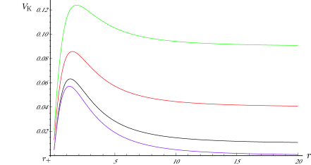
Figure 1: Various potentials as functions of $r$ for $M=2/3$, $a=\sqrt{3}/3$, $m=0.1$, and $r_{+}=1$. The bottom curve depicts the Kerr potential $V_{\rm K}(r)$, while three others are $V_{\rm K}^{\omega r,\omega M\ll 1}$ for $\omega=0.1,\leavevmode\nobreak\ 0.2,\leavevmode\nobreak\$and $0.3$ from bottom to top. For large $r$, it shows that $V_{\rm K}\to 0$, while $V_{\rm K}^{\omega r,\omega M\ll 1}\to\omega^{2}$.

It is shown that as $r\to\infty$, the potential $V_{\rm K}$ approaches $0$, while $V_{\rm K}^{\omega r,\omega M\ll 1}$ approaches $\omega^{2}$, which implies that its asymptotic behavior depends on the value of the frequency $\omega$. From Fig. 1, we observe a difference between $V_{\rm K}|_{r\to\infty}\to 0$ and $V_{\rm K}^{\omega r,\omega M\ll 1}|_{r\to\infty}\to\omega^{2}$ for large $r$. In the near-horizon of $r\approx r_{+}$, however, two potentials have the same form as

$$V_{\rm K}^{\omega r,\omega M\ll 1}\Big{|}_{r\approx r_{+}}=V_{\rm K}\Big{|}_{r\approx r_{+}}=\omega^{2}-(\omega^{2}-m\Omega)^{2}.$$ (3.7)

Their waves are given by solving (3.2) as

$$\psi_{+}=Ae^{-i(\omega-m\Omega)r^{*}}+Be^{i(\omega-m\Omega)r^{*}}.$$ (3.8)

It should be pointed out that the near-horizon region of $r\approx r_{+}$ is not enough to derive quasinormal modes because we have to impose boundary conditions at the horizon as well as asymptotic infinity. In order to describe the near-horizon region well, it is useful to introduce a new coordinate defined by

$$\rho=-\frac{1}{2\kappa}\ln\left[\frac{r-r_{+}}{r-r_{-}}\right],$$ (3.9)

where $r\in[r_{+},\infty)$ is inversely mapped into $\rho\in(\infty,0]$. In the near-horizon limit, we have a relation of $r\approx r_{+}+2r_{0}e^{-2\kappa\rho}$ which leads to $r\approx r_{+}$ for $\rho(=-r^{*})\to\infty$. Using this new coordinate, the radial equation (2) leads to the Schrödinger equation

$$\frac{d^{2}}{d\rho^{2}}R(\rho)+\Big{(}\omega^{2}-V_{\rm K}(\rho)\Big{)}R(\rho)=0,$$ (3.10)

where the potential $V_{\rm K}(\rho)$ is given by

$$V_{\rm K}(\rho)=\omega^{2}-\frac{\kappa^{2}}{\sinh^{2}[\kappa\rho]}\tilde{K}_{\ell}(\rho)$$ (3.11)

with $\tilde{K}_{\ell}(\rho)$

$$\tilde{K}_{\ell}(\rho)\leavevmode\nobreak\ =\leavevmode\nobreak\ \frac{\sinh^{2}[\kappa\rho]}{r_{0}^{2}}\Bigg{[}\Big{(}(M+r_{0}\coth[\kappa\rho])^{2}+a^{2}\Big{)}\omega-am\Bigg{]}^{2}$$

$$\hskip 170.00026pt+\leavevmode\nobreak\ 2ma\omega-a^{2}\omega^{2}-K_{\ell}.$$ (3.12)

We note that in the Schwarzchild limit ($a\to 0$), the potential (3.11) reduces to

$$V_{\rm K}^{a\to 0}(\rho)\to\omega^{2}\Bigg{[}1-\frac{1}{16e^{-4\kappa\rho}\sinh^{4}[\kappa\rho]}\Bigg{]}+\frac{\ell(\ell+1)\kappa^{2}}{\sinh^{2}[\kappa\rho]},$$ (3.13)

which is exactly the same as found in Ref.[13]. On the other hand, our main concern is to take the low-frequency and near-horizon limits in (3.11), which yields a simple potential form (see Appendix A for explicit derivation)

$$V_{\rm K}^{\omega M\ll 1}(\rho)\leavevmode\nobreak\ \approx\leavevmode\nobreak\ \Big{[}\omega^{2}-(\omega-m\Omega)^{2}\Big{]}+\frac{\ell(\ell+1)\kappa^{2}}{\sinh^{2}[\kappa\rho]}.$$ (3.14)

Here, the first term of (3.14) appears as a new term when comparing $V_{\rm K}^{\omega M\ll 1}$ with those for the Schwarzschild black hole [13] and the RN black hole [16]. Note that this term disappears for either the non-rotating black hole ($a=0$) or axisymmetric perturbation ($m=0$) [6].

Consequently, in the low-frequency and near-horizon limits the Eq.(3.10) together with (3.14) leads to the Schrödinger-like equation

$$\frac{d^{2}}{d\rho^{2}}R(\rho)+\Big{[}(\omega-m\Omega)^{2}-V_{\rm HCS}(\rho)\Big{]}R(\rho)=0,$$ (3.15)

where the HCS-potential $V_{\rm HCS}$ is given by [13, 16]

$$V_{\rm HCS}=\frac{\ell(\ell+1)\kappa^{2}}{\sinh^{2}[\kappa\rho]}.$$ (3.16)

It should be pointed out that Eq. (3.15) is the same forms obtained for the Schwarzschild and RN black holes when replacing $(\omega-m\Omega)^{2}$ by $\omega^{2}$, which implies that the potential $V_{\rm HCS}$ behaves as the potential of a scalar field around the AdS black hole because $V_{\rm HCS}\to\infty$ at asymptotic infinity ($\rho\to 0$). In the next section, we will use Eq. (3.15) to construct the new SL(2,R) three vector fields based on the $\rho$-representation for the Kerr black hole.

4 Quasinormal frequencies by operator method

First, we wish to derive QNFs of scalar around the Kerr black hole by employing an algebraic method based on the hidden conformal symmetry (2.8)-(2.13) [19]. For convenience, we identify $L_{n}=-iH_{n}$ and $\bar{L}_{n}=-i\bar{H}_{n}$, so that the $L_{n}$’s and $\bar{L}_{n}$ satisfy the Witt algebra, respectively,

$$[L_{n},L_{m}]=(n-m)L_{n+m},\leavevmode\nobreak\ \leavevmode\nobreak\ [\bar{L}_{n},\bar{L}_{m}]=(n-m)\bar{L}_{n+m}.$$ (4.1)

We first consider the primary state $\Phi^{(0)}$ with the conformal weight $h_{L}$ and $h_{R}$

$$L_{0}\Phi^{(0)}=h_{L}\Phi^{(0)},\leavevmode\nobreak\ \leavevmode\nobreak\ \bar{L}_{0}\Phi^{(0)}=h_{R}\Phi^{(0)}.$$ (4.2)

Acting operations $L_{0}$ and $\bar{L}_{0}$ on $\Phi^{(0)}$ with the ansatz

$$\Phi^{(0)}=e^{-i\omega_{0}t+im\phi}R^{(0)}(r)S(\theta),$$ (4.3)

then equation (4.2) yields the relation between $\omega$ and $m$ as

$$\omega_{0}=\frac{am}{2Mr_{+}}=m\Omega,$$ (4.4)

when requiring the same conformal weight condition $h_{L}=h_{R}$. In this case, $h_{L}$ and $h_{R}$ are determined to be

$$h_{L}=h_{R}=\frac{iam}{r_{+}}=2iM\omega_{0}.$$ (4.5)

As a result, from (2.22) and (4.5), the frequency $\omega_{0}$ is given by purely imaginary quantity

$$\omega_{0}=-i\frac{\ell+1}{2M}$$ (4.6)

and also, the azimuthal number $m$ becomes purely imaginary quantity

$$m=\frac{\omega_{0}}{\Omega}=-i2\pi(T_{R}+T_{L})(\ell+1).$$ (4.7)

In addition, the highest weight condition is implemented by requiring two conditions on scalar $\Phi^{(0)}$

$$L_{1}\Phi^{(0)}=\bar{L}_{1}\Phi^{(0)}=0.$$ (4.8)

It turns out that the solution to (4.8) is given by

$$\Phi^{(0)}(t,r,\phi)\leavevmode\nobreak\ =\leavevmode\nobreak\ C\Big{(}r^{2}+2(M-r)r_{-}-a^{2}\Big{)}^{-i\frac{m}{4\pi(T_{R}+T_{L})}}e^{-i\omega_{0}t+im\phi}$$ (4.9)

where $C$ is an integration constant. Staring from the highest weight state $\Phi^{(0)}$, we may construct all descendants $\Phi^{(n)}$ by using the relations

$$\Phi^{(n)} = e^{-i\omega_{n}t+im_{n}\phi}R^{(n)}(r)S(\theta)$$ (4.10)

$$= (\bar{L}_{-1})^{n}\Phi^{(0)}.$$

$\omega_{n},\leavevmode\nobreak\ m_{n}$, and $R^{(n)}$ are determined to give

$$\omega_{n} = \omega_{0}-i\frac{n}{2M}\leavevmode\nobreak\ =\leavevmode\nobreak\ -i\frac{1}{2M}(\ell+1+n),$$ (4.11)

$$m_{n} = -i2\pi T_{R}(\ell+1)-i2\pi T_{\rm L}(\ell+1+n),$$ (4.12)

$$R^{(n)}(r) = \triangle^{-\frac{n}{2}}\Big{(}-\triangle\partial_{r}-iam_{n-1}+i2Mr\omega_{n-1}\Big{)}$$ (4.13)

$$\times\triangle^{-\frac{n}{2}}\Big{(}-\triangle\partial_{r}-iam_{n-2}+i2Mr\omega_{n-2}\Big{)}$$

$$\times\cdots\times\triangle^{-\frac{n}{2}}\Big{(}-\triangle\partial_{r}-iam_{0}+i2Mr\omega_{0}\Big{)}R^{(0)}(r),$$

where $R^{(0)}(r)$ is given by

$$R^{(0)}(r)\leavevmode\nobreak\ =\leavevmode\nobreak\ C\Big{(}r^{2}+2(M-r)r_{-}-a^{2}\Big{)}^{-i\frac{m}{4\pi(T_{R}+T_{L})}},$$ (4.14)

which can be read off from (4.9). Even though we obtain QNFs and QNMs from $L_{n}$ and $\bar{L}_{n}$, their results are not promising because neither Eq. (4.11) is usual complex QNFs nor Im$[\omega_{n}]\propto 2\pi T_{H}$, compared with the QNFs [29] obtained for near extremal Kerr black holes (see Appendix B).

Now we turn to derive QNFs and QNMs of scalar around the Kerr black hole by using (3.15), which results from taking near-horizon as well as low-frequency limit. This suggests that QNFs and QNMs of scalar around the Kerr black hole may be obtained when replacing $\omega^{2}$ by $(\omega-m\Omega)^{2}$ in the Schwarzschild and RN black holes. It is straightforward to derive QNFs by introducing three vector fields

$$L_{1} = \frac{1}{\kappa}e^{\kappa t}\Big{[}\cosh\left(\kappa\rho\right)\partial_{t}+\sinh\left(\kappa\rho\right)\partial_{\rho}\Big{]}\ ,$$

$$L_{0} = -\frac{1}{\kappa}\partial_{t}\ ,$$ (4.15)

$$L_{-1} = \frac{1}{\kappa}e^{-\kappa t}\Big{[}\cosh\left(\kappa\rho\right)\partial_{t}-\sinh\left(\kappa\rho\right)\partial_{\rho}\Big{]}\ .$$

These satisfy the SL(2,R) commutation relations

$$\left[L_{0},L_{\pm 1}\right]=\mp L_{\pm 1},\leavevmode\nobreak\ \leavevmode\nobreak\ \leavevmode\nobreak\ \left[L_{1},L_{-1}\right]=2L_{0}.$$ (4.16)

Then, the SL(2,R) Casimir operator is constructed by

$${\cal H}_{\rho}^{2} = L^{2}_{0}-\frac{1}{2}(L_{1}L_{-1}+L_{-1}L_{1})$$ (4.17)

$$= -\Big{(}\frac{\sinh(\kappa\rho)}{\kappa}\Big{)}^{2}\partial^{2}_{t}+\Big{(}\frac{\sinh(\kappa\rho)}{\kappa}\Big{)}^{2}\partial^{2}_{\rho}\ .$$

Eq.(3.15) could be written as

$${\cal H}_{\rho}^{2}\tilde{\Phi}(\rho)=\ell(\ell+1)\tilde{\Phi}(\rho),$$ (4.18)

where $\tilde{\Phi}$ can be effectively written as

$$\tilde{\Phi}(t,\rho,\theta)\sim e^{-i(\omega_{0}-m\Omega)t}R(\rho)S(\theta).$$ (4.19)

First of all, we define the primary state by $\Phi^{(0)}$ which satisfies

$$L_{0}\tilde{\Phi}^{(0)}=h\tilde{\Phi}^{(0)},$$ (4.20)

and the highest weight condition

$$L_{1}\tilde{\Phi}^{(0)}=0.$$ (4.21)

Considering (4.19), one has a conformal weight

$$h=i\frac{\omega_{0}-m\Omega}{\kappa}=i\frac{\omega_{0}-m\Omega}{2\pi T_{H}}.$$ (4.22)

On the other hand, for $\tilde{\Phi}^{(0)}$, the SL(2,R) Casimir operator satisfies

$${\cal H}^{2}\tilde{\Phi}^{(0)}=h(h-1)\tilde{\Phi}^{(0)}.$$ (4.23)

Comparing Eq. (4.23) with Eq. (4.18), one has

$$h=\frac{1}{2}[1\pm(2\ell+1)].$$ (4.24)

Together with Eq. (4.22), for $h>0$, one can find

$$\omega_{0}=m\Omega-i2\pi T_{H}(\ell+1).$$ (4.25)

Then, all the descendants are constructed by

$$\tilde{\Phi}^{(n)}=(L_{-1})^{n}\tilde{\Phi}^{(0)}$$ (4.26)

so that we have

$$\tilde{\Phi}^{(n)}\equiv e^{-i(\omega_{n}-m\Omega)t}R^{(n)}(\rho).$$ (4.27)

Here we read off QNFs as

$$\omega_{n}=\omega_{0}-i\kappa n=m\Omega-i2\pi T_{H}\Big{[}n+\ell+1\Big{]},$$ (4.28)

which is one of our main results.

Moreover, the $n$-th radial eigenfunction $R^{(n)}(\rho)$ takes the form

$$R^{(n)}(\rho) = \left(\kappa\right)^{-n}\left(-i(\omega_{n-1}-m\Omega)\cosh\left(\kappa\rho\right)-\sinh\left(\kappa\rho\right)\frac{d}{d\rho}\right)$$ (4.29)

$$\leavevmode\nobreak\ \times\left(-i(\omega_{n-2}-m\Omega)\cosh\left(\kappa\rho\right)-\sinh\left(\kappa\rho\right)\frac{d}{d\rho}\right)$$

$$\leavevmode\nobreak\ \cdot\cdot\cdot\times\left(-i(\omega_{0}-m\Omega)\cosh\left(\kappa\rho\right)-\sinh\left(\kappa\rho\right)\frac{d}{d\rho}\right)R^{(0)}(\rho).$$

We also have

$$L_{0}\tilde{\Phi}^{(n)}=(h+n)\tilde{\Phi}^{(n)},$$ (4.30)

which implies that $\tilde{\Phi}^{(n)}$ forms a principal discrete highest weight representation of the SL(2,R). Now we wish to solve the highest weight condition (4.21) to determine the highest weight state $R^{(0)}(\rho)$

$$\Big{[}-i(\omega_{0}-m\Omega)\cosh\left(\kappa\rho\right)+\sinh\left(\kappa\rho\right)\frac{d}{d\rho}\Big{]}R^{(0)}(\rho)=0.$$ (4.31)

The solution is given by

$$R^{(0)}(\rho)=C\Big{[}\sinh\left(\kappa\rho\right)\Big{]}^{i\frac{\omega_{0}-m\Omega}{\kappa}}.$$ (4.32)

We note that the solution (4.32) behaves as

$$R^{(0)}\sim e^{-i(\omega_{0}-m\Omega)r_{*}}\leavevmode\nobreak\ \leavevmode\nobreak\ \leavevmode\nobreak\ \leavevmode\nobreak\ \leavevmode\nobreak\ {\rm for}\leavevmode\nobreak\ \leavevmode\nobreak\ r\rightarrow r_{+}.$$ (4.33)

This is the ingoing mode propagating into the horizon ($\rho\to\infty$). For the $n$-th radial eigenfunction, one can easily show by induction

$$R^{(n)}\sim e^{-i(\omega_{n}-m\Omega)r_{*}},\leavevmode\nobreak\ \leavevmode\nobreak\ {\rm as}\leavevmode\nobreak\ r_{*}\to-\infty.$$ (4.34)

Finally, we observe that $R^{(0)}(0)=0$ at infinity ($\rho\rightarrow 0,r_{*}\to\infty)$, which shows that it is not the outgoing wave at infinity but satisfies the Dirichlet boundary condition as like at the infinity of AdS spacetime. Moreover, the first radial eigenfunction $R^{(1)}(\rho)$ can be explicitly constructed as

$$R^{(1)}(\rho)=-2iC(\omega_{0}-m\Omega)\cosh(\kappa\rho)\Big{[}\sinh\left(\kappa\rho\right)\Big{]}^{i\frac{\omega_{0}-m\Omega}{\kappa}},$$ (4.35)

which also satisfies the Dirichlet boundary condition at infinity. One can easily show that the $n$-th radial eigenfunction $R^{(n)}(\rho)$ behaves as the same way as $R^{(1)}(\rho)$ likewise.

5 Near-horizon geometry of the NEK black hole

In the case of Kerr black hole spacetime imposed by hidden conformal symmetry, it is conjectured that the specified black hole spacetime could be the near-horizon region of a NEK black hole with $a\to M$. In this section we wish to study the near-horizon geometry of the NEK black hole and obtain QNFs of scalar propagating around this background geometry. For this purpose, we first consider the NEK black hole by considering the conditions of $r_{0}\ll 1,\leavevmode\nobreak\ a\approx M,$ and $r_{+}\approx r_{-}\approx M$ which are explicitly expressed by introducing a very small parameter $\lambda$ as [32]

$$r_{\pm} = M\pm r_{0}\approx M\pm 2\pi M\tilde{T}_{R}\lambda+{\cal O}(\lambda^{2})$$ (5.1)

$$a = \sqrt{r_{+}r_{-}}\approx M-2M(\lambda\pi\tilde{T}_{R})^{2}+{\cal O}(\lambda^{3}),$$ (5.2)

which imply that three temperatures and angular velocity are approximated to be

$$T_{L}\approx\frac{1}{2\pi},\leavevmode\nobreak\ \leavevmode\nobreak\ T_{R}\approx\frac{r_{0}}{2\pi M}\approx\tilde{T}_{R}\lambda,\leavevmode\nobreak\ \leavevmode\nobreak\ T_{\rm NEK}\approx\frac{r_{0}}{4\pi M^{2}}\approx\frac{\tilde{T}_{R}\lambda}{2M},\leavevmode\nobreak\ \leavevmode\nobreak\ \Omega\approx\frac{1}{2M}.$$ (5.3)

Here one is keeping $\tilde{T}_{R}$ fixed in the limits of $T_{\rm NEK},T_{R}\to 0(\lambda\to 0)$ and it is called the dimensionless near-horizon temperature. In order to describe the near-horizon geometry, we also introduce three coordinates

$$\tau=\lambda\frac{t}{2M},\leavevmode\nobreak\ \leavevmode\nobreak\ \leavevmode\nobreak\ y=\frac{r-r_{+}}{\lambda r_{+}},\leavevmode\nobreak\ \leavevmode\nobreak\ \leavevmode\nobreak\ \varphi=\phi-\frac{t}{2M},$$ (5.4)

and take $\lambda\to 0$ keeping $(\tau,y,\varphi)$ fixed. After some manipulations, we obtain the near-horizon region of NEK black hole isolated by the NHEK limit [33]

$$ds^{2}=2J\Gamma(\theta)\Bigg{[}-y(y+4\pi\tilde{T}_{R})d\tau^{2}+\frac{dy^{2}}{y(y+4\pi\tilde{T}_{R})}+d\theta^{2}+\Lambda^{2}\Big{(}d\varphi+(y+2\pi\tilde{T}_{R})d\tau\Big{)}^{2}\Bigg{]},$$

(5.5)

where

$$\Gamma(\theta)=\frac{1+\cos^{2}\theta}{2},\leavevmode\nobreak\ \leavevmode\nobreak\ \leavevmode\nobreak\ \leavevmode\nobreak\ \leavevmode\nobreak\ \Lambda(\theta)=\frac{2\sin\theta}{1+\cos^{2}\theta}$$

with $\theta\in[0,\pi]$ and $\varphi\sim\varphi+2\pi$. The horizon is located at $y=0$. For the extremal Kerr black hole, we have $\tilde{T}_{R}=0$ and its near-horizon geometry is described by

$$ds^{2}_{\rm NHEK}=2J\Gamma(\theta)\Bigg{[}-y^{2}d\tau^{2}+\frac{dy^{2}}{y^{2}}+d\theta^{2}+\Lambda^{2}\Big{(}d\varphi+yd\tau\Big{)}^{2}\Bigg{]}$$ (5.6)

in terms of Poincare coordinates. This represents the quotient of warped AdS${}_{3}\approx$ AdS${}_{2}\times S^{1}$ for fixed polar angle $\theta$ [34]. Hence, the presence of $\tilde{T}_{R}$ distinguishes between NEK and extremal Kerr black holes.

It is found that in the background spacetime (5.5), the massless Klein-Gordon equation $\nabla_{\mu}\nabla^{\mu}\Phi=0$ with

$$\Phi(\tau,y,\theta,\varphi)=e^{-i\tilde{\omega}\tau+im\varphi}Y(y)S(\theta)$$ (5.7)

can be decomposed into two differential equations

$$\left[\frac{1}{\sin\theta}\partial_{\theta}(\sin\theta\partial_{\theta})-\frac{m^{2}}{\sin^{2}\theta}-\frac{m^{2}}{4}\sin^{2}\theta+\bar{K}_{\ell m}\right]S(\theta)=0$$ (5.8)

and

$$\Bigg{[}\partial_{y}\Big{(}y(y+4\pi\tilde{T}_{R})\partial_{y}\Big{)}-\bar{K}_{\ell m}+m^{2}+\frac{\Big{(}\tilde{\omega}+m(y+2\pi\tilde{T}_{R})\Big{)}^{2}}{y(y+4\pi\tilde{T}_{R})}\Bigg{]}Y(y)=0,$$ (5.9)

where $\bar{K}_{\ell m}$ are eigenvalues which can be computed numerically [33]. Approximately, it is given by $\bar{K}_{\ell m}\approx\ell(\ell+1)+cm^{2}$ with $c\in[0.13,0.22]$ and $\ell\geq|m|$. We now introduce a coordinate defined by

$$dy^{*}=\frac{dy}{y(y+4\pi\tilde{T}_{R})},$$ (5.10)

which is integrated to be

$$y^{*}=\frac{1}{4\pi\tilde{T}_{R}}\ln\Big{[}\frac{y}{y+4\pi\tilde{T}_{R}}\Big{]}.$$ (5.11)

This maps $y\in[0,\infty)$ to $y^{*}\in(-\infty,0]$. Then, the equation (5.9) becomes the Schrödinger-type equation

$$\frac{d^{2}Y}{dy^{*2}}+\Big{(}\tilde{\omega}^{2}-V_{\rm NEK}(y)\Big{)}Y=0.$$ (5.12)

The potential $V_{\rm NEK}(y)$ is given by

$$V_{\rm NEK}(y)=\tilde{\omega}^{2}+(\bar{K}_{\ell m}-m^{2})y(y+4\pi\tilde{T}_{R})-\Big{(}\tilde{\omega}+m(y+2\pi\tilde{T}_{R})\Big{)}^{2},$$ (5.13)

which implies that $\lim_{y\to\infty}V_{\rm NEK}\to\infty$ for $\ell>|m|$. This reflects the nature of AdS₂ base in (5.5). In other words, the case of $\ell=m$ is not allowed for our computation.

On the other hand, in the near-horizon limit, it takes the form

$$V_{\rm NEK+}(y)\leavevmode\nobreak\ \approx\leavevmode\nobreak\ \tilde{\omega}^{2}-(\tilde{\omega}+2\pi\tilde{T}_{R}m)^{2},$$ (5.14)

which leads to zero for $m=0$. In this case, a solution to (5.12) is given by

$$Y_{+}(y^{*})=Ae^{-i(\tilde{\omega}+2\pi\tilde{T}_{R}m)y^{*}}+Be^{i(\tilde{\omega}+2\pi\tilde{T}_{R}m)y^{*}},$$ (5.15)

where the first term (the second one) correspond to the ingoing mode (outgoing mode) when considering (5.7). We are now in a position to find QNFs of scalar field around the black hole (5.5). It turns out that the solution to Eq.(5.9) is given by the hypergeometric functions as

$$Y(y) = c_{1}y^{-\frac{i}{2}\left(m+\frac{\tilde{\omega}}{2\pi\tilde{T}_{R}}\right)}(y+4\pi\tilde{T}_{R})^{-\frac{i}{2}\left(m-\frac{\tilde{\omega}}{2\pi\tilde{T}_{R}}\right)}\times$$ (5.16)

$${}_{2}F_{1}\Big{[}-im+\frac{1}{2}+\beta,\leavevmode\nobreak\ -im+\frac{1}{2}-\beta,\leavevmode\nobreak\ 1-i\left(m+\frac{\tilde{\omega}}{2\pi\tilde{T}_{R}}\right),\leavevmode\nobreak\ -\frac{y}{4\pi\tilde{T}_{R}}\Big{]}$$

$$+\leavevmode\nobreak\ c_{2}y^{\frac{i}{2}\left(m+\frac{\tilde{\omega}}{2\pi\tilde{T}_{R}}\right)}(y+4\pi\tilde{T}_{R})^{-\frac{i}{2}\left(m-\frac{\tilde{\omega}}{2\pi\tilde{T}_{R}}\right)}\times$$

$${}_{2}F_{1}\Big{[}\frac{i\tilde{\omega}}{2\pi\tilde{T}_{R}}+\frac{1}{2}+\beta,\leavevmode\nobreak\ \frac{i\tilde{\omega}}{2\pi\tilde{T}_{R}}+\frac{1}{2}-\beta,\leavevmode\nobreak\ 1+i\left(m+\frac{\tilde{\omega}}{2\pi\tilde{T}_{R}}\right),\leavevmode\nobreak\ -\frac{y}{4\pi\tilde{T}_{R}}\Big{]}$$

where $c_{1,2}$ are arbitrary constants and $\beta$ is given by

$$\beta=\sqrt{\frac{1}{4}+\bar{K}_{\ell m}-2m^{2}}.$$ (5.17)

We note that the two first terms ($c_{1}y^{\cdot},c_{2}y^{\cdot}$) can be recovered from considering (5.15) together with (5.11).

In order to obtain QNFs, we first require the ingoing mode at horizon and then, Dirichlet boundary condition at infinity. Choosing the ingoing mode at horizon $(y=0)$ leads to $c_{2}=0$ and then, the solution at infinity ($y\to\infty$) can be written as

$$Y(y)=\Gamma_{1}y^{-\frac{1}{2}-\beta}+\Gamma_{2}y^{-\frac{1}{2}+\beta},$$ (5.18)

where $\Gamma_{1,2}$ are given by

$$\Gamma_{1} = c_{1}\frac{\Gamma(-2\beta)\Gamma\Big{[}1-i(m+\frac{\tilde{\omega}}{2\pi T_{R}})\Big{]}}{\Gamma(-im+\frac{1}{2}-\beta)\Gamma(-i\frac{\tilde{\omega}}{2\pi\tilde{T}_{R}}+\frac{1}{2}-\beta)},$$ (5.19)

$$\Gamma_{2} = c_{1}\frac{\Gamma(2\beta)\Gamma\Big{[}1-i(m+\frac{\tilde{\omega}}{2\pi\tilde{T}_{R}})\Big{]}}{\Gamma(-im+\frac{1}{2}+\beta)\Gamma(-i\frac{\tilde{\omega}}{2\pi T_{R}}+\frac{1}{2}+\beta)}.$$ (5.20)

Imposing the Dirichlet condition at infinity leads to $\Gamma_{2}=0$, which provides two conditions

$$-im+\frac{1}{2}+\beta=-n,$$ (5.21)

$$-i\frac{\tilde{\omega}}{2\pi\tilde{T}_{R}}+\frac{1}{2}+\beta=-n.$$ (5.22)

From (5.22), one finds the purely imaginary QNFs

$$\tilde{\omega}=-i2\pi\tilde{T}_{R}\Big{(}n+\frac{1}{2}+\beta\Big{)}.$$ (5.23)

Further, considering the transformation (5.4), we have the relation of time and angular-part

$$e^{-i\omega t+im\phi}=e^{-i\tau[\frac{2M}{\lambda}\omega-\frac{m}{\lambda}]+im\varphi}=e^{-i\tau\tilde{\omega}+im\varphi},$$ (5.24)

which implies that QNFs are given by

$$\omega=m\Omega-i2\pi T_{\rm NEK}\Big{(}n+\frac{1}{2}+\beta\Big{)}.$$ (5.25)

Also, we have

$$\omega_{R}=\omega,\leavevmode\nobreak\ \leavevmode\nobreak\ T_{R}=2MT_{\rm NEK}.$$ (5.26)

From (5.21), one has

$$m=-i2\pi T_{L}\Big{(}n+\frac{1}{2}+\beta\Big{)},$$ (5.27)

which implies that azimuthal number $m$ is purely imaginary for real $\beta>0$.

Finally, we wish to mention that for $\ell\gg m$, $\beta$ is approximated to be

$$\beta=\sqrt{\ell(\ell+1)+1/4-(2-c)m^{2}}\approx\ell+\frac{1}{2},$$ (5.28)

which allows us to rewrite $\omega$ as

$$\omega\approx m\Omega-i2\pi T_{\rm NEK}\Big{(}n+\ell+1\Big{)},$$ (5.29)

being consistent with the result (4.28) for a nearly extremal case of replacing $T_{H}$ by $T_{\rm NEK}$.

6 Summary and conclusion

QNFs	Eq. (4.28)	Eq. (5.25)	Eq. (6.19)
background		near-horizon geometry
geometry	Kerr	of NEK	NEK
		(asymptotically AdS)	(asymptotically flat)
how to		boundary conditions:	boundary conditions:
find	operator	ingoing mode (near horizon)	ingoing mode (near horizon)
QNFs	method	0       (at infinity)	outgoing mode (at infinity)
permitted			non-equatorial:
QN modes	all	$\ell\gg m$	$\ell\neq m\geq 0$
taking	near-horizon
the limit	near-region	no limit	near-region
further	nearly
restriction	extremal	no further restriction	no further restriction
final
QNFs	$\omega\simeq m\Omega-i2\pi T_{\rm NEK}(n+\ell+1)$

Table 1: Comparison between the QNFs approaches

In this paper, we have obtained two analytic expressions for QNFs:
   (i)  (4.28), found by using the hidden conformal symmetry developed in the near-horizon,
   (ii) (5.25), obtained considering the near-horizon geometry of the NEK black hole.
The reference QNFs (6.25) was shown in Appendix B, which are those of non-equatorial ($\ell\not=m$) scalar modes around the NEK black hole. They are different apparently, but it was shown that QNFs (i) correspond approximately to not only those (5.29) of scalar perturbation around the near-horizon region of NEK black hole, but also those (6.25) of non-equatorial ($\ell\not=m$) scalar modes around the NEK black hole.

On the other hand, the hidden conformal symmetry approach based on (2.8)-(2.13) with the potential (3.6) in the near-region could not determine QNFs of scalar around the NEK black hole, while QNFs (i) indicates that the hidden conformal symmetry by using (3.15) given in the near-horizon region as well as near-region provides the same as QNFs (5.29) for the nearly extremal case.

We mention that the approaches (i) and (ii) do not yield QNFs (6.26) of equatorial $(\ell=m$) modes around the NEK black hole. This is because the hidden conformal symmetry and near-horizon geometry approaches keep the near-horizon feature of the scalar potential around the NEK black hole only (see Table 1). It should be pointed out that $\delta^{2}$ (6.15) always take a negative value in the near-region and low-frequency limits, which implies that the equatorial mode ($\delta^{2}>0$) and near-region limit are incompatible to each other. That is why the approaches (i) and (ii), obtained from the near-region and near horizon, do not admit the long-lived equatorial mode.

Finally, we conclude that the hidden Kerr/CFT proposal could determine quasinormal modes and frequencies of the massless scalar wave propagating around the NEK (rapidly rotating) black hole partly.

Appendix A: Explicit derivation of (3.14)

We first arrange the potential (3.11) as

$$V_{\rm K}(\rho) = \omega^{2}-\frac{\kappa^{2}}{\sinh^{2}[\kappa\rho]}\tilde{K}_{\ell}(\rho)$$ (6.1)

$$= \omega^{2}-\Bigg{[}\frac{\kappa}{r_{0}}\Big{(}(M+r_{0}\coth[\kappa\rho])^{2}+a^{2}\Big{)}\omega-\frac{\kappa}{r_{0}}am\Bigg{]}^{2}$$

$$\hskip 110.00017pt-\leavevmode\nobreak\ \frac{2\kappa^{2}ma\omega}{\sinh^{2}[\kappa\rho]}+\frac{\kappa^{2}a^{2}\omega^{2}}{\sinh^{2}[\kappa\rho]}+\frac{\kappa^{2}K_{\ell}}{\sinh^{2}[\kappa\rho]}.$$

In the low frequency ($\omega a,\leavevmode\nobreak\ \omega M\ll 1$) and near-horizon limits, the second line of Eq. (6.1) becomes

$$\omega^{2}-\Bigg{[}\frac{\kappa}{r_{0}}\Big{(}(M+r_{0}\coth[\kappa\rho])^{2}+a^{2}\Big{)}\omega-\frac{\kappa}{r_{0}}am\Bigg{]}^{2}$$ (6.2)

$$\Rightarrow \omega^{2}-\Bigg{[}\frac{\kappa}{r_{0}}\Big{(}(M+r_{0})^{2}+a^{2}\Big{)}\omega-\frac{\kappa}{r_{0}}am\Bigg{]}^{2}$$

$$= \omega^{2}-\Bigg{[}\frac{\kappa}{r_{0}}\Big{(}r_{+}^{2}+a^{2}\Big{)}\omega-\frac{\kappa}{r_{0}}am\Bigg{]}^{2}$$

$$= \omega^{2}-(\omega-m\Omega)^{2},$$ (6.3)

where we used $r_{+}=M+r_{0}$ in (6.2) and $\kappa=r_{0}/(r_{+}^{2}+a^{2})=r_{0}\Omega/a$ in (6.3). A dominant term in the third line of Eq. (6.1) is given by

$$\frac{\kappa^{2}K_{\ell}}{\sinh^{2}[\kappa\rho]}=\frac{\ell(\ell+1)\kappa^{2}}{\sinh^{2}[\kappa\rho]}.$$ (6.4)

From (6.3) and (6.4), we finally obtain (3.14).

Appendix B: QNFs of NEK black holes

In this Appendix we briefly show an analytic form of QNFs of scalar around NEK black holes in asymptotically flat spacetime [30, 29]. To this end, we first recall the radial equation (2) which is reexpressed in terms of $k=r^{2}\omega+a^{2}\omega-am$ as

$$\triangle\frac{\partial^{2}R}{\partial r^{2}}+2(r-M)\frac{\partial R}{\partial r}+\left(\frac{k^{2}}{\triangle}+2ma\omega-a^{2}\omega^{2}-K_{\ell}\right)R=0.$$ (6.5)

Introducing new dimensionless variables

$$x=\frac{r-r_{+}}{r_{+}},\leavevmode\nobreak\ \leavevmode\nobreak\ \leavevmode\nobreak\ \bar{\tau}=\frac{2r_{0}}{r_{+}},\leavevmode\nobreak\ \leavevmode\nobreak\ \leavevmode\nobreak\ \bar{\omega}=\frac{\omega-m\Omega}{2\pi T_{H}},\leavevmode\nobreak\ \leavevmode\nobreak\ \leavevmode\nobreak\ \hat{\omega}=\omega r_{+},$$ (6.6)

(6.5) can be rewritten as

$$x(x+\bar{\tau})R^{\prime\prime}+(2x+\bar{\tau})R^{\prime}+WR=0,$$ (6.7)

where the prime (${}^{\prime})$ denotes differentiation with respect to $x$ and $W$ is

$$W=\frac{k^{2}}{x(x+\bar{\tau})r_{+}^{2}}+2ma\omega-a^{2}\omega^{2}-K_{\ell}.$$ (6.8)

We mention that the double limit of $a\to M$ and $\omega\to m\Omega$ correspond to $\bar{\tau}\to 0$ and $\bar{\omega}\to 0$. The former limit indicates the NEK black hole, while the latter shows that $\omega_{R}$ is almost given by $m\Omega$ in the NEK black hole. Note also that for QNMs, two boundary conditions near the horizon and at infinity are given by

$$R\sim\left\{\begin{array}[]{ll}(i)\leavevmode\nobreak\ \leavevmode\nobreak\ {\rm\leavevmode\nobreak\ ingoing\leavevmode\nobreak\ waves\leavevmode\nobreak\ }\hskip 25.50006pt{\rm as}\leavevmode\nobreak\ \leavevmode\nobreak\ x\to 0\leavevmode\nobreak\ \leavevmode\nobreak\ (r\to r_{+}),\\ (ii)\leavevmode\nobreak\ {\rm\leavevmode\nobreak\ outgoing\leavevmode\nobreak\ waves\leavevmode\nobreak\ }\hskip 20.00003pt{\rm as}\leavevmode\nobreak\ \leavevmode\nobreak\ x\to\infty\leavevmode\nobreak\ \leavevmode\nobreak\ (r\to\infty).\end{array}\right.$$ (6.11)

In the far region ($x\gg{\rm max}\{\bar{\tau},\bar{\omega}\}$), (6.7) becomes

$$x^{2}R^{\prime\prime}+2xR^{\prime}+W_{\rm far}R=0,$$ (6.12)

where

$$W_{\rm far}=\omega^{2}r_{+}^{2}x^{2}+4\omega\hat{\omega}r_{+}x+4\hat{\omega}^{2}+2ma\omega-a^{2}\omega^{2}-K_{\ell}.$$ (6.13)

A solution to (6.12) is expressed in terms of the confluent hypergeometric function,

$$R_{\rm far} = A_{1}(2i\omega r_{+})^{\frac{1}{2}+i\delta}x^{-\frac{1}{2}+i\delta}e^{-i\omega r_{+}x}\leavevmode\nobreak\ U(i\delta+2i\hat{\omega}+1/2,\leavevmode\nobreak\ 1+2i\delta,\leavevmode\nobreak\ 2i\omega r_{+}x)$$ (6.14)

$$+A_{2}(2i\omega r_{+})^{\frac{1}{2}-i\delta}x^{-\frac{1}{2}-i\delta}e^{-i\omega r_{+}x}\leavevmode\nobreak\ U(-i\delta+2i\hat{\omega}+1/2,\leavevmode\nobreak\ 1-2i\delta,\leavevmode\nobreak\ 2i\omega r_{+}x),$$

where an important quantity $\delta$ is given by

$$\delta^{2}=4\hat{\omega}^{2}+2ma\omega-a^{2}\omega^{2}-K_{\ell}-\frac{1}{4},$$ (6.15)

which is either positive or negative. Here $K_{\ell}$ is given by

$$K_{\ell}=\ell(\ell+1)+{\cal O}(a\omega).$$ (6.16)

On the other hand, in near-horizon region ($x\ll 1$), (6.7) reduces to

$$x(x+\bar{\tau})R^{\prime\prime}+(2x+\bar{\tau})R^{\prime}+W_{\rm near}R=0,$$ (6.17)

where $W_{\rm near}$ is

$$W_{\rm near}=\frac{(2\hat{\omega}x+\bar{\omega}\bar{\tau}/2)^{2}}{x(x+\bar{\tau})}+2ma\omega-a^{2}\omega^{2}-K_{\ell}.$$ (6.18)

Imposing the ingoing boundary condition $(i)$ in (6.11), one finds a solution to (6.17) as

$$R_{\rm near}=x^{-\frac{i}{2}\bar{\omega}}\left(\frac{x}{\bar{\tau}}+1\right)^{i(\bar{\omega}/2-2\hat{\omega})}{}_{2}F_{1}(i\delta-2i\hat{\omega}+1/2,\leavevmode\nobreak\ -i\delta-2i\hat{\omega}+1/2\leavevmode\nobreak\ 1-i\bar{\omega},\leavevmode\nobreak\ -x/\bar{\tau}),$$ (6.19)

where ${}_{2}F_{1}$ is the hypergeometric function. A remaining task is to match solution (6.14) with (6.19) in the overlapping region ${\rm max}\{\bar{\tau},\bar{\omega}\}\ll x\ll 1$. It turns out that this matching condition determines $A_{1}$ and $A_{2}$ to be

$$A_{1} = \bar{\tau}^{-\frac{i}{2}\bar{\omega}+\frac{1}{2}-i\delta}(2i\omega r_{+})^{-\frac{1}{2}-i\delta}\frac{\Gamma(2i\delta)\Gamma(1-i\bar{\omega})}{\Gamma(i\delta+\frac{1}{2}-2i\hat{\omega})\Gamma(i\delta+\frac{1}{2}+2i\hat{\omega}-i\bar{\omega})},$$ (6.20)

$$A_{2} = \bar{\tau}^{-\frac{i}{2}\bar{\omega}+\frac{1}{2}+i\delta}(2i\omega r_{+})^{-\frac{1}{2}+i\delta}\frac{\Gamma(-2i\delta)\Gamma(1-i\bar{\omega})}{\Gamma(-i\delta+\frac{1}{2}-2i\hat{\omega})\Gamma(-i\delta+\frac{1}{2}+2i\hat{\omega}-i\bar{\omega})}.$$ (6.21)

Substituting (6.20) and (6.21) into (6.14), and imposing the outgoing boundary condition $(ii)$ in (6.11), we get the quasinormal condition

$$\frac{\Gamma(2i\delta)\Gamma(1+2i\delta)(-2i\bar{\tau}\hat{\omega})^{-i\delta}}{[\Gamma(i\delta+\frac{1}{2}-2i\hat{\omega})]^{2}\Gamma(i\delta+\frac{1}{2}-i\bar{\omega}+2i\hat{\omega})}=-\frac{\Gamma(-2i\delta)\Gamma(1-2i\delta)(-2i\bar{\tau}\hat{\omega})^{i\delta}}{[\Gamma(-i\delta+\frac{1}{2}-2i\hat{\omega})]^{2}\Gamma(-i\delta+\frac{1}{2}-i\bar{\omega}+2i\hat{\omega})}.$$

After manipulations with taking the double limits of $\bar{\tau},\bar{\omega}\ll 1$, we find the QNFs of scalar around NEK black hole for non-equatorial ( $\ell\neq m\geq 0$) modes with $\delta^{2}<0$ [29]

$$\omega\simeq m\Omega-i2\pi T_{\rm NEK}\Big{[}n+\frac{1}{2}-i\delta\Big{]},\leavevmode\nobreak\ \leavevmode\nobreak\ \Omega=\frac{1}{2M},\leavevmode\nobreak\ \leavevmode\nobreak\ T_{\rm NEK}=\frac{r_{0}}{4\pi M^{2}}\ll 1.$$ (6.22)

In the low-frequency limit of $\omega a\leq\omega M\ll 1$ and $\hat{\omega}=\omega r_{+}\ll 1$ for the NEK black hole, $\delta^{2}$ is negative as

$$\delta^{2}\simeq-\frac{1}{4}-\ell(\ell+1)$$ (6.23)

and thus, $\delta$ is given by

$$\delta=i\Big{(}\ell+\frac{1}{2}\Big{)}.$$ (6.24)

Plugging $\delta$ into (6.22) leads to

$$\omega\simeq m\Omega-i2\pi T_{\rm NEK}\Big{(}n+\ell+1\Big{)},$$ (6.25)

which is the same form as in (4.28) for a nearly extremal case and as in (5.29).

On the other hand, for equatorial $\ell=m\geq 0$ modes with $\delta^{2}>0$, their QNFs take an approximate form

$$\omega\simeq m\Omega-i2\pi T_{\rm NEK}\Big{(}n+\frac{1}{2}\Big{)},$$ (6.26)

which implies that non-equatorial modes decay faster than equatorial modes.

References

- [1] A. Castro, A. Maloney and A. Strominger, Phys. Rev. D 82, 024008 (2010) [arXiv:1004.0996 [hep-th]].
- [2] C. Krishnan, JHEP 1007, 039 (2010) [arXiv:1004.3537 [hep-th]].
- [3] M. Cvetic and F. Larsen, Nucl. Phys. B 506, 107 (1997) [hep-th/9706071].
- [4] M. Cvetic and F. Larsen, JHEP 1202, 122 (2012) [arXiv:1106.3341 [hep-th]].
- [5] M. Guica, T. Hartman, W. Song and A. Strominger, Phys. Rev. D 80, 124008 (2009) [arXiv:0809.4266 [hep-th]].
- [6] G. Compere, Living Rev. Rel. 15, 11 (2012) [arXiv:1203.3561 [hep-th]].
- [7] I. Bredberg, C. Keeler, V. Lysov and A. Strominger, Nucl. Phys. Proc. Suppl. 216, 194 (2011) [arXiv:1103.2355 [hep-th]].
- [8] B. Chen and J. Long, Phys. Rev. D 82, 126013 (2010) [arXiv:1009.1010 [hep-th]].
- [9] A. Castro, J. M. Lapan, A. Maloney and M. J. Rodriguez, Class. Quant. Grav. 30 (2013) 165005 [arXiv:1304.3781 [hep-th]].
- [10] M. Cvetic and G. W. Gibbons, arXiv:1312.2250 [gr-qc].
- [11] S. Bertini, S. L. Cacciatori and D. Klemm, Phys. Rev. D 85, 064018 (2012) [arXiv:1106.0999 [hep-th]].
- [12] E. Berti, V. Cardoso and A. O. Starinets, Class. Quant. Grav. 26, 163001 (2009) [arXiv:0905.2975 [gr-qc]].
- [13] Y. -W. Kim, Y. S. Myung and Y. -J. Park, Phys. Rev. D 87, 024018 (2013) [arXiv:1210.3760 [hep-th]].
- [14] R. A. Konoplya and A. Zhidenko, Rev. Mod. Phys. 83, 793 (2011) [arXiv:1102.4014 [gr-qc]].
- [15] T. Ortin and C. S. Shahbazi, Phys. Lett. B 716, 231 (2012) [arXiv:1204.5910 [hep-th]].
- [16] Y. -W. Kim, Y. S. Myung and Y. -J. Park, Eur. Phys. J. C73, 2440 (2013) [arXiv:1205.3701 [hep-th]].
- [17] C. -M. Chen, S. P. Kim, I-C. Lin, J. -R. Sun and M. -F. Wu, Phys. Rev. D 85, 124041 (2012) [arXiv:1202.3224 [hep-th]].
- [18] R. Cordero, A. Lopez-Ortega and I. Vega-Acevedo, Gen. Rel. Grav. 44, 917 (2012) [arXiv:1201.3605 [gr-qc]].
- [19] D. A. Lowe, I. Messamah and A. Skanata, Phys. Rev. D 84, 024030 (2011) [arXiv:1105.2035 [hep-th]].
- [20] D. A. Lowe and A. Skanata, J. Phys. A 45, 475401 (2012) [arXiv:1112.1431 [hep-th]].
- [21] J. E. McClintock, R. Shafee, R. Narayan, R. A. Remillard, S. W. Davis and L. -X. Li, Astrophys. J. 652, 518 (2006) [astro-ph/0606076].
- [22] J. E. McClintock and R. A. Remillard, arXiv:0902.3488 [astro-ph.HE].
- [23] G. Risaliti, F. A. Harrison, K. K. Madsen, D. J. Walton, S. E. Boggs, F. E. Christensen, W. W. Craig and B. W. Grefenstette et al., arXiv:1302.7002 [astro-ph.HE].
- [24] S. A. Teukolsky, Phys. Rev. Lett. 29, 1114 (1972);
- [25] S. A. Teukolsky and W. H. Press, Astrophys. J. 193, 443 (1974).
- [26] S. L. Detweiler, Astrophys. J. 239, 292 (1980).
- [27] M. Sasaki and T. Nakamura, Gen. Rel. Grav. 22, 1351 (1990).
- [28] N. Andersson and K. Glampedakis, Phys. Rev. Lett. 84, 4537 (2000) [gr-qc/9909050].
- [29] S. Hod, Phys. Rev. D 78, 084035 (2008) [arXiv:0811.3806 [gr-qc]].
- [30] V. Cardoso, Phys. Rev. D 70, 127502 (2004) [gr-qc/0411048].
- [31] H. Yang, F. Zhang, A. Zimmerman, D. A. Nichols, E. Berti and Y. Chen, Phys. Rev. D 87, 041502 (2013) [arXiv:1212.3271 [gr-qc]].
- [32] I. Bredberg, T. Hartman, W. Song and A. Strominger, JHEP 1004, 019 (2010) [arXiv:0907.3477 [hep-th]].
- [33] J. M. Bardeen and G. T. Horowitz, Phys. Rev. D 60, 104030 (1999) [hep-th/9905099].
- [34] Y. -W. Kim, Y. S. Myung and Y. -J. Park, Eur. Phys. J. C67, 533 (2010) [arXiv:0901.4390 [hep-th]].